The Renormalization Group for Large-Scale Structure: Origin of Galaxy Stochasticity
Abstract
The renormalization group equations for large-scale structure (RG-LSS) describe how the bias and stochastic (noise) parameters—both of matter and biased tracers such as galaxies—evolve as a function of the cutoff of the effective field theory. In previous work, we derived the RG-LSS equations for the bias parameters using the Wilson-Polchinski framework. Here, we extend these results to include stochastic contributions, corresponding to terms in the effective action that are higher order in the current . We show that the RG equations exhibit an interesting, previously unnoticed structure at all orders in , which implies that a single nonlinear bias term immediately generates all stochastic moments through RG evolution. We then derive the nonlinear RG evolution of the (leading-derivative) stochastic parameters for all -point functions, and show that this evolution is controlled by a different, lower scale than the nonlinear scale. This has implications for the optimal choice of the renormalization scale when comparing the theory with data to obtain cosmological constraints.
1 Introduction
Galaxy redshift surveys map out the large-scale structure (LSS) over a substantial part of the observable low-redshift universe, and constitute a rich source of information on gravity, dark matter, dark energy, and the initial conditions of structure formation. To unlock this information, however, one has to marginalize over the significant uncertainties in our understanding of galaxy formation. What is required in particular is a reliable prediction for the conditional probability of forming a galaxy that passes observational luminosity and color selections, at a given location. The effective field theory (EFT) approach [1, 2, 3, 4, 5, 6], built upon cosmological perturbation theory, allows for a consistent expansion of the galaxy density field into operators , ranked in terms of perturbative order, and corresponding bias coefficients as well as stochastic contributions. The latter can be effectively described by a field and coefficients (see [7] for a review):
| (1.1) |
We emphasize that at the level of the partition function, there is no stochastic field , as we will see below. Nevertheless, the field and its statistics are useful to give physical meaning to the stochastic terms appearing in the partition function.111Note that we only write a single field in Eq. (1.1), unlike the previous literature which has introduced multiple fields . We will discuss this distinction in more detail in upcoming work.
When computing observable statistics such as -point correlation functions based on Eq. (1.1) (technically these involve expectation values of products of composite operators), loop integrals arise which have to be regularized. The standard approach has so far been to work at the level of -point correlation functions, and to remove the UV-sensitive loop integrals via counterterms [8, 9]. In this paper, following up on [10] (henceforth “Paper 1”), our aim is instead to pursue the renormalization-group (RG) approach of Wilson [11] and Polchinski [12], which proceeds by integrating out small-scale modes in the partition function, and which we refer to as “RG-LSS” in the following. Ref. [3] was the first to point out how this approach can be adapted to the EFT of LSS. Ref. [13] used it to derive the EFT prediction for the conditional probability density of the galaxy field given the matter density field; that is, the crucial ingredient needed for making predictions for galaxy clustering, as noted above.
The Wilson-Polchinski approach to renormalization proceeds by integrating out modes in the free field above a momentum cutoff .222The Wilson-Polchinski approach is often referred to as nonperturbative [14, 15, 16], in contrast to Wilson’s pioneering perturbative approach. In the LSS case, this corresponds to integrating modes above the cutoff in the linear density field. Integrating out modes in a thin shell in momentum space leads to renormalization-group equations that govern the running of the coupling constants in the effective action, such as the bias coefficients (“RG flow”). In Paper 1, we explicitly derived the RG equations governing the running of the bias coefficients, and showed that the basis of bias operators used there is closed under renormalization. The bias coefficients describe the mean-field prediction for the galaxy density given a realization of large-scale perturbations. However, the small-scale modes that have been integrated out also lead to scatter around this mean-field relation, which we refer to as stochasticity. In this paper, we turn to these stochastic contributions to the galaxy density field, which are described by interaction terms in the effective action that involve second and higher powers of the current. We derive how nonlinear bias sources such stochastic contributions when integrating out modes, and describe the general hierarchy that governs the RG flow between different types of interactions in the effective action.
The outline of the paper is as follows. In the remainder of this section, we summarize the main results and define our notation. In Sec. 2 we discuss the partition function that includes the most general set of stochastic operators as higher-order-in- terms. We derive in Sec. 3 the general RG flow for the terms in the bias expansion including stochasticity. Sec. 4 presents results for those RG equations and discusses their numerical solutions. We conclude in Sec. 5. App. A is dedicated to the evaluation of the shell integrals, while App. B proves which shell diagrams need to be included in the RG flow.
1.1 Summary of main results
The main formal result of the paper is a general renormalization group equation (RGE) for stochastic contributions to galaxy clustering. Stochasticity corresponds to contributions to the effective action that are higher-order in the current , i.e. with . The general effective action for the galaxy density field is given in Eq. (2.2)
| (1.2) |
Note that the set of operators appearing here is always the same, and terms with are nothing but the bias expansion with . We explain how generates the -point functions of galaxy clustering after Eq. (2.7). Expanding the operator functionals in Eq. (1.2) [as discussed in more detail below, cf. Eq. (1.18)], we recover the effective action introduced by [3]
| (1.3) |
with each representing a sum over operator kernels with associated coefficients .333Specifically, we have (1.4) where the sum runs over all bias operators contributing at order and is defined in Eq. (1.18). The fact that Ref. [3] considered a special case of biased tracer, matter, is not important for the structure of the equations. Ref. [3] then derive RG equations for the coefficient tensors [Eq. (4.22) there; notice that in their notation, and are swapped and their corresponds to our ]. For clarity, let us drop all indices and combinatorial factors in the following. The structure of the RGE derived by Ref. [3] is
| (1.5) |
where , the derivative of the cut linear power spectrum with respect to the cutoff, stands for the inverse propagator, or covariance of linear modes in the infinitesimal momentum shell , and denotes index contractions, i.e. momentum integrals. In the lower line of Eq. (1.5), we have written the corresponding Feynman diagrams illustrating the modes in the momentum shell that are being integrated out (red wiggly lines; for our complete Feynman conventions, see Sec. 1.2).
We will argue in this paper that the second term in Eq. (1.5) in fact vanishes in general due to kinematics. Instead, the general RG-LSS equation becomes
| (1.6) |
where the series continues to all orders in . While one might think that terms with higher powers of are suppressed since one is considering a narrow shell in momentum space, this is not the case as we will show (hint: all terms in Eq. (1.6) are one-loop diagrams). Note that for (bias terms), only the first term in both Eq. (1.5) and Eq. (1.6) contributes, and we recover the RGE for bias parameters studied in detail in Paper 1.
Clearly, the structure of Eq. (1.6) is quite different from, and more complex than that of Eq. (1.5). We will explain in detail how Eq. (1.6) arises, and what the physical ramifications are. The main results are the following:
-
•
Eq. (1.6) implies that, under RG flow, a single nonlinear bias term such as immediately generates terms of any order in the current; that is, it generates all moments of stochasticity.
-
•
The finding that terms of order in the effective action do not source terms with (in particular, stochasticity does not source bias terms) remains valid.
-
•
Despite the seemingly complicated structure of Eq. (1.6), we are able to derive an explicit closed form valid at any order in [Eq. (3.36)]. This is possible thanks to the specific, simple structure of the diagrams involved: going to higher order in amounts to inserting another factor of given by lower-order kernels .
-
•
Finally, we express Eq. (1.6) as an explicit set of nonlinear ordinary differential equations for the stochastic amplitudes, given the bias coefficients as a function of scale. This nonlinearity leads to interesting behavior under RG flow, and ramifications for the choice of the renormalization scale in EFT analyses, which we investigate in Sec. 4.
1.2 Notation
We follow a similar notation to Paper 1, which we review here.
For the Fourier conventions, we use and for momenta variables where bold letters represent three-vectors and as a short notation for the sum of vectors. We also use prime in the subscript or in the variable interchangeably, e.g. . Fourier-space integrals are written as
| (1.7) |
The corresponding real-space normalization is
| (1.8) |
We denote fields smoothed with a sharp-k filter on a length scale as , where, in Fourier space,
| (1.9) |
We define an operator of order as a function of insertions of the matter overdensity
| (1.10) |
Here we adopt for the Dirac delta. We also use as the bias basis of operators
| Zeroth order: | ||||
| First order: | ||||
| Second order: | ||||
| Third order: | (1.11) |
Notice that we included the zeroth-order unit operator , which starts to contribute at order since the term leads to a tadpole contribution that is subtracted after setting . In Fourier space, the unit operator is a Dirac delta. The Galileon operators are defined as
| (1.12) | |||||
| (1.13) |
with being the scaled gravitational potential. At third order we have
| (1.14) |
that also contains , the velocity potential. Moreover, we define
| (1.15) |
In order to avoid tadpole contributions, we normalize (starting from first-order operators)
| (1.16) |
We further expand the matter density field as
| (1.17) |
where are the usual PT kernels (with ) [17] such that
| (1.18) |
One can derive the by inserting Eq. (1.17) into Eq. (1.10). We also use . Therefore, we can more generically write or simply the shorthand notation . The three types of vertices are represented by
| (1.19) |
where the large boxes indicate the operator convolution Eq. (1.10) or Eq. (1.18) and the small boxes represent the expansion of , Eq. (1.17). The linear density-field legs are represented as dashed lines.
We write down the partition function
| (1.20) |
where is the effective action (see Sec. 2) and
| (1.21) |
the probability distribution function (PDF) of the Gaussian field .
We consider two types of propagators: the linear propagator cut at
| (1.22) |
and the shell propagator that only has support within an infinitesimal shell in momentum space
| (1.23) |
Those propagators are represented as
We also use the shorthand prime notation
| (1.24) |
Finally, the variance of the linear density field is defined as
| (1.25) |
For the effective stochastic field, we can define the leading stochastic contribution to -point functions as
| (1.26) | ||||
| (1.27) | ||||
| (1.28) |
The higher-derivative stochasticity can be defined in real space as, for instance for ,
| (1.29) |
We will discuss this further in the next section. The stochastic cross-moment involving an operator can be defined as, for instance
| (1.30) |
or more generally
| (1.31) |
As an important point here, notice that any correlator involving a single instance of vanishes, i.e. does not correlate linearly with any of the other operators:
| (1.32) |
We stress again that these relations mainly serve to give meaning to the coefficients and in general; the partition function is completely written in terms of these coefficients and without reference to .
We use a Planck 2018 Euclidean CDM cosmology [18] for all numerical results.
2 The general EFT partition function for bias and stochastic parameters
The focus of this section is to generalize the partition function of Paper 1,
| (2.1) |
beyond the leading stochastic contributions considered there. Here, the sum runs over all bias operators that are relevant at a given order in perturbations and derivatives.444For other works on the large-scale structure partition function, see also [19, 20, 21, 22, 13]. Notice that Eq. (2.1) includes a nonlinear coupling between the field and the current , via the operators . Terms that couple nonlinearly to the current are usually referred to as “composite operators” (see [23, 24] and the books [25, 26]). As discussed in [23], the renormalization of those composite operators will lead to terms that are higher-order in . As we will see in Sec. 3, those higher-order stochastic contributions are necessary to obtain a partition function that remains consistent under the RG flow. Thus, the general effective action, writing explicitly the terms of Eq. (2.1), is given by a sum over local-in-space products of currents and bias operators
| (2.2) |
where we include the trivial constant operator in the set of bias operators, which is more convenient when going to higher order in . We can then identify as the bias parameters555Notice that the tadpole coefficient after setting . at the scale , and as the second-order “Gaussian” stochastic amplitudes, with corresponding to the well-known stochastic or “shot noise” contribution to the galaxy power spectrum. Similarly, quantifies the leading coupling of stochasticity to the density (“density-dependent shot noise”). However, Eq. (2.2) also includes non-Gaussian stochastic contributions, starting at with as the purely stochastic contribution to the galaxy bispectrum.
Notice that the interactions among the and in Eq. (2.2) are purely local. This is a consequence of working at leading order in derivatives for the stochastic contributions. Higher-derivative contributions, such as and are also present in general, and are expected to be controlled by the same scale as that controlling the higher-derivative bias operators. We will neglect them in the following, however.
It is useful to study the dimension of each coefficient . Let the dimension of a given be ; for an operator that is leading-order in derivatives666We count the number of derivative with respect to the density field . E.g., has , while has . we have , while higher-derivative operators will have . Then, by dimensional analysis
| (2.3) | ||||
| (2.4) | ||||
| (2.5) |
The Fourier-space -point correlation function of a biased tracer is given by
| (2.6) |
which can be obtained by taking derivatives of the partition function with respect to , evaluated at :
| (2.7) |
We find for instance
| (2.8) | ||||
| (2.9) | ||||
| (2.10) | ||||
where we have used Eq. (1.16) for all operators apart from . This structure continues similarly toward higher order. Notice that these expressions are valid at any loop order in the perturbative expansion in . Thus, from the structure of the -point functions, we can read off that the corresponds to the -th moment of the (purely) stochastic contribution to the galaxy density field. This term first appears in the -point function as a -independent contribution, whereas the other coefficients appear in -point functions with .
3 RG flow via the partition function
In this section, we derive the RG flow equations based on the Wilson-Polchinski formalism, which explicitly integrates out high-momentum modes in the partition function. We generalize the bias RG equations developed in Paper 1 to include stochastic parameters for all higher -point functions. We discuss the general structure of the running of the bias and stochastic parameters for all -point functions. The reader interested in the main conclusions of this section can skip directly to Sec. 3.4.
3.1 Integrating out a momentum shell via Wilson-Polchinski
In this section we follow the same procedure described by [3, 10], splitting the integration functional between two cutoffs and
| (3.1) |
in which is a field that has support only in an infinitesimal shell of width . The partition function, written in real space, becomes
| (3.2) | |||
where is the real-space current, i.e., the Fourier transform of . Notice that we chose the current to have support only at and not and therefore the partition function on the LHS also has support only up to . This is essential in the derivation, as it guarantees that the current is orthogonal to ,
| (3.3) |
This of course still allows for the evaluation of the partition function (and therefore the -point functions derived from it) at momenta lower than (see Paper 1 for a broader discussion). We can then expand the operator , that is, evaluated at -th order in perturbation theory, into contributions with different powers of :777For instance, the expansion of can be written as (3.4) For other examples of this expansion, see Appendix A.1 of Paper 1.
After integrating out the momentum shell, we find
| (3.6) |
where each of the corrections from the shell modes, is of order . The correction is given by
| (3.7) |
as already pointed out in Paper 1. The correction, , is given by
| (3.8) | |||
where we see that terms appear. Finally, the correction is
| (3.9) | |||
We highlight again that terms proportional to (i.e., the bias operators) in general source etc. operators. The terms proportional to (the Gaussian stochastic terms ) source , etc. terms. Therefore, each order in is only affected by powers of smaller than , as already pointed out by [3] for the matter case. Later, this will allow us to obtain a self-consistent solution of the RG evolution.
The single, double and triple-operator shell contraction , and are defined in Fourier space as
| (3.10) | ||||
| (3.11) | ||||
| (3.12) | ||||
The corresponding diagrams are shown in Figs. 1–3 below. Notice that we keep only the terms involving even powers of shell fields, given our assumption of Gaussian initial conditions, with
| (3.13) | ||||
General structure of partition function and its renormalization.
Let us consider the part of the effective action Eq. (2.2) that involves precisely powers of the current, and compute how the correction renormalizes the coefficients. We have:
| (3.14) |
where, again, is the stochastic coefficient of -th order in , related to the -th cumulant of the stochasticity. The correction at -th order in currents can be written as a sum in the number of operators that are being contracted, where for each we sum over the contributions :
| (3.15) |
where
| (3.16) |
is a symmetry factor in which is the number of times appears in ; hence, , , , , , , and so forth. Notice that we isolated a factor in the first line of Eq. (3.15) for reasons that will become clear in Sec. 3.4. Eq. (3.15) is the master equation that will guide the following sections. One can trivially recover Eq. (3.7), Eq. (3.8) and Eq. (3.9) for respectively. On the other hand, it is important to stress the difference with respect to Eq. (4.22) of [3], which only includes the contributions of the type and . Crucially, as we will see later and already anticipated in Eq. (3.15), we find that the only relevant contributions come from shell contributions , while the term is actually suppressed due to its kinetic structure and the orthogonality with the current .
3.2 On the corrections to [ in Eq. (3.15)]
The contributions from enter generically in the correction of all coefficients defined in Eq. (3.15) when taking . As example, we calculate the correction to the coefficients , but that contribution in fact appears for any coefficient . We display the first diagrams in Fig. 1, in which we see the 1-loop diagram (left) and the diagram (right), the last being suppressed as described in App. A.2.
The terms.
We begin with the most general structure of RG contributions coming from . This part follows the derivations of Paper 1, but we reproduce it for completeness. In general, we can write for the operator
| (3.17) |
where is the contribution of the operator to via . We used the results of Paper 1, reproduced in App. A, in which we find that the single-operator shell integrals are proportional to after expanding
| (3.18) |
Therefore, the correction to from in Eq. (3.14) is given by
| (3.19) |
We can then identify
| (3.20) |
and after writing and taking , we can write
| (3.21) |
where the derivative of the variance is evaluated at . The set of coefficients is presented in Tab. 1, as described in App. A.1 and Paper 1.
| - | - | - | - | - | - | - | |
| - | - | 3 | - | - | |||
| - | - | - | - | ||||
| - | - | - | - | - |
A last interesting point to notice here is that the corrections of the type [ in Eq. (3.15)] do not generate contributions to the zeroth-order operator , i.e. the tadpole, which reflects the fact that for all operators. The terms are therefore only sourced by higher-order contributions starting from .
The (suppression of) and higher-order terms.
We dedicate App. A.2 to discuss how the contributions coming from a single operator but expanded in higher orders of shell fields (, , ) are suppressed by extra factors of compared to . Since we can take the limit without loss of generality of the RG flow, we can therefore drop these terms, and it is sufficient to consider in .
3.3 On the corrections to [ in Eq. (3.15)]
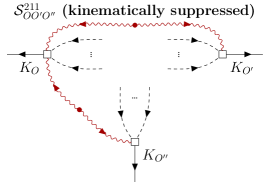
The double-operator shell contribution acts as a source to terms in the action, as well as higher-order terms, as one can see from Eq. (3.8). We consider the coefficients here as example. To keep the structure clear, in this section we keep only as a source of . The tree-level and 1-loop diagrams for the terms are shown in Fig. 2.
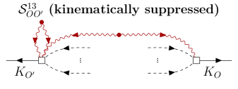
The main contributions from .
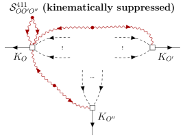
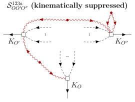
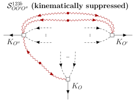
We start by discussing which of the diagrams described in Fig. 2 constitute the main stochastic contribution. In order to not overload the main text with the technical details, we dedicate App. B to show that both the tree-level term and the 1-loop term are zero due to their kinematic structure. This can already be seen from the top left and bottom diagrams in Fig. 2: all dashed incoming lines to the involve , and are thus constrained to have momenta . On the other hand, the outgoing lines are constrained by the support of the current factors , i.e. by the external momenta . In the limit of , there is a vanishing amount of phase space available for momenta in the shell (wiggly lines) in this kinematic configuration. Hence, these contributions cannot form the dominant source of stochastic terms.
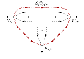
Instead, the leading contribution comes from the term. This was in fact already anticipated in Eq. (3.13) of [13]. As is apparent from the the top right diagram in Fig. 2, the kinematic suppression does not apply in this case, as two modes with momenta in the shell can couple to produce an external momentum . In fact, this is a specific case of the generic conclusion of App. B.2 that the terms of the type are the leading sources in general. To exemplify this, we show the corresponding tree-level and 1-loop diagrams for the terms in Fig. 3.
Corrections to and .
We now focus on contributions to zeroth and first-order leading-in-derivative () operators and . Since these contributions will exemplify the general structure of RG source terms, we go into a bit more technical detail here. Readers only interested in the final result can skip ahead to Eq. (3.34).
In this work we focus only on contributions sourced by up to second-order operators. We show in App. A.3 that, when neglecting operators starting from third-order the only of the diagrams that contributes to those operators is via
| (3.22) |
Using the result of Eq. (A.28), we find that the leading contribution of to the zeroth-order operator is
| (3.23) |
with corrections of order , which are absorbed by higher-derivative stochastic contributions. Despite the fact that this correction involves four powers of , it is linear order in , i.e. of the same order as , since
| (3.24) |
Following Eq. (3.8), this yields a correction to the term
| (3.25) |
which reads
| (3.26) |
where in the second line we used and we introduced the shell contribution , which determines the contribution of to . Moreover, it scales as expected from dimensional analysis (recall that has dimensions of power spectrum, i.e. length cubed). Therefore, following the same steps as Eq. (3.20), we find
| (3.27) |
We now move to the corrections to the first-order operator . As calculated in Eq. (A.32), we find that the contribution of to the term in the effective action is
| (3.28) |
after using Eq. (3.38) and defining , that determines the contribution of to . Similarly, using Eq. (A.33) and Eq. (A.34)
| (3.29) | ||||
| (3.30) |
with and . Following Eq. (3.8), those terms yield a correction to
| (3.31) |
that reads
| (3.32) |
Therefore, considering only the contributions we find
| (3.33) |
3.4 The general source structure from the master equation [Eq. (3.15)]
One can easily show using Eq. (3.15) that we can construct the general system of ODEs for all the bias and stochastic parameters to be
| (3.36) |
where is the contribution of the operators to via . In addition to the and , described in Tab. 1 and Eq. (3.35), we now have
| (3.37) |
as calculated in App. A.4. Notice that the prefactor is simply a permutation factor and only will appear in the final ODEs. Another key fact is that terms contribute all at the same order (i.e. linearly in ) as a consequence of
| (3.38) |
that generalizes Eq. (3.24), such that
| (3.39) | |||||
Notice the specific scaling of each contribution with different powers of , which is required by dimensional analysis [Eq. (2.5)].
Let us consider the zeroth-order stochastic contributions , which correspond to the moments of the effective stochastic field [Eq. (1.28)]. We find that the only contribution comes from [noticing that the contribution after removing the tadpole using Eq. (1.16)], leading to
| (3.40) |
This leads to an important conclusion: the presence of the operator in the bias expansion immediately generates all , i.e. all moments of the stochasticity.
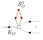
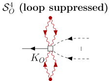
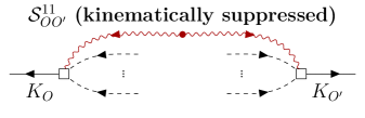
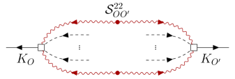
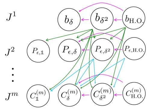
We display the structure of the RG source terms in Fig. 4. The columns show different operator orders, while the rows the different powers in . The arrows indicate which terms in the action are sourced by a given term .
3.5 Summary
We now summarize the main conclusions of this section, providing some insights into the structure of the general RG-LSS equation:
- •
-
•
In general, -th order stochastic moments contribute to -th order moments with . For example, bias terms () lead to runnning of bias coefficients as well as (in general) all stochastic contributions. For the specific case of , the terms are the only contribution. Both of these points were already noticed by [3]. For , we recover the results of Paper 1, which are represented by the first row in Fig. 4.
-
•
If all source terms to the RG equations were of the type, there would be no coupling between terms with different powers in the current, . In particular, no stochasticity () would be generated by nonlinear bias (). However, we find that terms of the form generate contributions of similar relevance as to all higher . That is, a single nonlinear bias term immediately generates all stochastic moments when running to a scale . This finding differs substantially from the conclusions of [3], who only considered and as relevant contributions. We find to be kinematically suppressed, while , and its generalization to operators, is unsuppressed.888Another elucidating and perhaps more familiar example of this type of contribution is the renormalization of that appears for the matter field, which sources a higher-derivative stochastic operator proportional to , and therefore absorbed by a term in the effective action.
- •
4 Results
After having provided the general set of equations for the running of bias and stochastic parameters in Eq. (3.36), we move to discuss their solutions. We separate the discussion into the different powers of .
: bias parameters.
For the case , we find that only the in Tab. 1 contribute, such that, following Paper 1
| (4.1) | ||||
| (4.2) | ||||
| (4.3) |
We use the notation for the parameters that are evaluated at a fixed renormalization scale and999Notice that we switched the parenthesis in Paper 1 for curly brackets in terms such as to avoid confusion with the coefficients.
| (4.4) | ||||
| (4.5) | ||||
| (4.6) |
to account for contributions from higher-order operators in a short-hand notation, in which quantifies the contributions of operators of order to via and . We refer to Paper 1 for a broader discussion on the approximation that considers those higher-order operators as constants evaluated at , as well as the analytical solution for the bias RGE. In particular, it was pointed out that it is important to include higher-order operators, but sufficient to approximate their coefficients as constants. Therefore, in order to avoid cluttering the text, hereafter we omit terms such as the last terms in Eqs. (4.1)–(4.3), that account for the truncation effect of approximating higher-order operators as constants.
: stochastic power spectra.
The running of the stochastic parameters is considered here (to our knowledge) for the first time in the LSS literature. We consider the equation for the first and zeroth-order terms. Recall that enters in the power spectrum, cf. Eq. (2.9), while appears in the bispectrum, cf. Eq. (2.10). We find that
| (4.7) | ||||
| (4.8) |
where the terms are the novel sources from . Notice an important simplification taken here, which involves fixing at . The complete evaluation of this term requires calculating with two external legs, as well as contributions involving third and fourth-order operators, which is beyond the scope of this paper. We define and similar to Eqs. (4.4)–(4.6) we defined
| (4.9) | ||||
| (4.10) |
to account for higher-order operators. Here, and account respectively for the , contributions to that have at least one operator that is third-order or higher. We also included another subscript to account for the number of operators in the contributing operator product. This is a generalization of the terms such as presented above, which includes contributions from multiple which appear starting from order .
: stochastic bispectra.
The terms start to contribute at the bispectrum level. We have
| (4.11) | ||||
| (4.12) | ||||
where we included the novel contribution from in the last lines of each ODE. We also define and
| (4.13) | ||||
| (4.14) | ||||
| (4.15) |
to account for higher-order operators for the stochastic term. Here, , and account respectively for the , and contributions to that have at least one operator that is third-order or higher.
Solutions and discussion.
First, we note the vertical coupling of the RGE, where the equations for bias terms, i.e. order , are independent of coefficients (see Fig. 4), and the equations for the coefficients are independent of the terms. This points to an iterative solution, starting with , and a consistent way to truncate the RGE hierarchy in powers of (as first observed in [3]). In addition to that truncation in , which corresponds to a truncation of the set of -point functions one is interested in, there are necessary truncations in terms of order of operators, and in terms of derivative orders , which are suppressed by . These truncations, which are discussed in Section 2 of Paper 1, remain similarly valid for the stochastic terms as well.
Note also that universal -independent coefficients appear in the RGE; for example, the prefactor multiplying in the RGE for , explicitly shown above for [see Eq. (4.1), Eq. (4.8) and Eq. (4.12)], which is a direct consequence of the same interaction kernels appearing in the same kinematic configuration in these contributions. Unfortunately, this does not mean we can make general predictions for relations between the , for example, because different high-order operators contribute to the running for each .
Moreover, whereas the bias parameters admit a variable change solving directly for , the source terms for the stochastic parameters are controlled by [see Eq. (3.36)]. The velocity with which those parameters run in the RG-flow is thus determined by how large is. An analytic solution to the RG-flow of terms starting from is not easily achievable due to the non-analytic form of . One could attempt to find solutions for power-law Universes or consider a FFTLog expansion of the CDM matter power spectra for that [27, 28], which we leave for future work.
In order to illustrate the RGE results, we consider the following scenario for the initial condition for the parameters, that we have seen appear in the source of stochastic operators, in which we fix
| (4.16) | ||||
| (4.17) | ||||
| (4.18) |
at (corresponding to the renormalization scale Mpc), while all others are set to zero at the same scale:
| (4.19) |
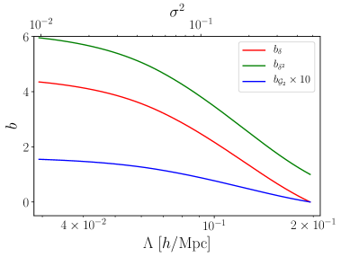
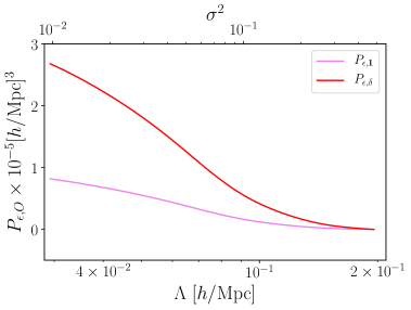
That situation corresponds to a case in which terms are responsible for populating all other operators. The solutions for this scenario are shown in Fig. 5. We show solutions for the (top left), (top right) and (bottom) parameters as a function of the scale . As discussed in Paper 1 and seen in Eqs. (4.1)–(4.3), the running of terms, when neglecting higher-order operators, is sourced by . For the terms, notice that despite those parameters starting from zero at , they rise sharply to . These dynamics can be explained through the shape of the CDM matter power spectrum, together with Eqs. (4.7)–(4.8). Parametrically, when running from a high scale to , the change in is given by
| (4.20) |
for a CDM power spectrum, explaining the order of magnitude seen in the figure [note that the contribution is controlled by , which likewise grows toward smaller and is not included in the estimate Eq. (4.20)]. Similarly,
| (4.21) |
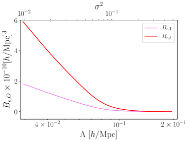
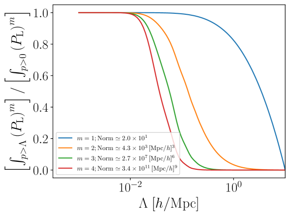
The reason for the rapid running is the shape of the linear matter power spectrum: both of the above integrals are in fact dominated by the lowest wavenumbers, close to (as long as is greater than the turnover scale in the power spectrum, ). A similarly enhanced contribution dominated by IR modes was pointed out for the matter four-point function in [29]. This is in contrast to the corresponding integral appearing in the RGE for bias parameters, which is controlled by the variance of the linear density field, , and is dominated by UV modes. The dominance of low- modes in fact grows as one considers higher , i.e. higher stochastic moments. This is illustrated in Fig. 6. In hindsight, this behavior is not surprising: Eqs. (4.20)–(4.21) give the expected order of magnitude of those operators since is the only dimensionful quantity that appears in the RG equations at leading order in derivatives.
These results have interesting implications for the choice of the renormalization scale when attempting to model the clustering of actual LSS tracers: choosing a low cutoff means that stochastic amplitudes will be enhanced, reducing the effective signal-to-noise of the measurement (recall that the stochastic terms also appear in the covariance, i.e. the likelihood of -point functions). Thus, one should attempt to increase to the highest scale still amenable to a perturbative description. We aim to investigate the optimal choice for the renormalization scale in a future work.
It is further worth highlighting that
| (4.22) |
meaning that if at one fixed we have , as physically required since it corresponds to a variance, then this coefficient will remain positive for all . To see why this is physically required, consider the case of a tracer with vanishing . The power spectrum [Eq. (2.10)], which has to be non-negative, is then on large scales.
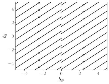
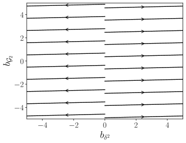
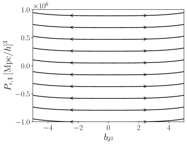
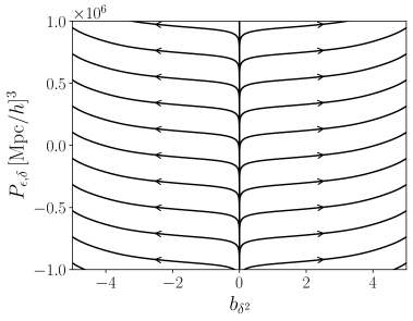
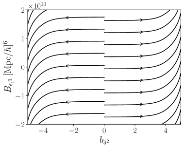
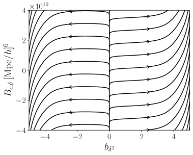
Let us now move beyond the simple initial conditions considered for Fig. 5, Eq. (4.18). We display in Fig. 7 the RG-flow of different parameters as a function of . The top, middle and bottom panels present respectively the , and terms. Here, we focus on a 2-d slice in the multidimensional parameter space that describes the running. Each line points towards the direction , with different initial conditions in the respective planes shown, with and and the other parameters, not shown in the respective figures, set to zero in the limit . Note that the running of is much stronger than that of , as expected and already shown in Fig. 2 of Paper 1. For the running of the in the second row, presented in this work for the first time, we note especially the inflection point visible for , which can be understood as a competition between the (from ) and (from ) in Eq. (4.8). For the terms in the last row, we see a complex structure in the RG-flow emerging from the different terms in Eq. (4.11) and Eq. (4.12).
5 Conclusion
We have used the general effective action for large-scale structure, Eq. (2.2), to derive the “RG-LSS” equations which describe the running of bias and stochastic contributions to the clustering of LSS tracers under a change of the renormalization scale. This extends the analysis of Paper 1 [10], which focused on bias, i.e. terms linear in the current , to arbitrary powers of . In Sec. 3, we make use of the Wilson-Polchinski formalism to derive how those terms are sourced by bias operators and lower-order-in- stochastic parameters. We provide a very general master formula Eq. (3.36) for the evolution of a general stochastic parameter as a function of the cutoff , which simplifies to Eq. (3.40) for the shot-noise contributions to -point functions. We also analyse in Sec. 4 solutions to the RG-flow including stochastic parameters.
In this work we continue to follow the philosophy introduced in Paper 1, which keeps the smoothing cutoff (i.e., the renormalization scale) finite, instead of subtracting the leading order contributions by taking the large-scale limit as considered in usual EFT of LSS analyses. The finite- allows for the derivation of the RG equations using the Wilson-Polchinski framework, which may account for a yet-to-be-determined amount of extra information from the resummation of part of higher-loop contributions as in the usual context of quantum field theory. We find that, different than for the bias parameters, the RG group equations for the stochastic parameters are nonlinear, which may suggest that some relevant information may be absorbed by the their RG flow. Furthermore, non-trivial critical points may arise from the RG flow structure of the bias and stochastic parameters. These are directions we aim to investigate in the future. Another interesting generalization to be understood in light of the RG equations is the presence of primordial non-Gaussianities. Non-Gaussianities lead to new types of vertices for which the RG equations (and their inbuilt resummation) may be relevant.
Acknowledgments
HR is supported by the Deutsche Forschungsgemeinschaft under Germany’s Excellence Strategy EXC 2094 ‘ORIGINS’. (No. 390783311). We thank Giovanni Cabass, Mathias Garny, Charalampos Nikolis, and Marko Simonovic for discussions and Charalampos Nikolis and Beatriz Tucci for feedback on the paper.
Appendix A Evaluation of shell integrals including relevant contributions for the stochastic terms
In this appendix, we focus on calculating the shell integrals , and . We direct the reader to Appendix A.1 of Paper 1 for a complete form of the shell operators Eq. (3.1).
A.1 The integrals
We start reviewing part of the results of Appendix A of Paper 1, in which
| (A.1) |
is calculated. We split the calculation in terms of the number of external legs
| (A.2) |
in which, e.g., corresponds to corrections to , corresponds to corrections to , corresponds to corrections to second-order operators as
Contributions from .
The contribution leads to
| (A.3) |
and then, e.g.,
| (A.4) |
which would contribute to . This contribution, however, is removed after the normalization Eq. (1.16). The other two zero-leg contributions come from and which lead to
| (A.5) | |||||
| (A.6) |
Contributions from .
The only terms that contribute to the running of leading in derivatives single-leg operators are those from , and shell-integrals
| (A.7) | |||||
| (A.8) | |||||
| (A.9) |
Contributions from .
Omitting terms that only contribute to higher-derivative operators, we find
| (A.10) | |||||
| (A.11) | |||||
| (A.12) |
Notice that part of those terms also contribute to one-leg terms found above with the same coefficients, as a consequence of the equivalence principle [10].
Fourth-order operators also introduce contributions of the type , e.g.
| (A.13) |
We leave the calculation of the full contribution of the set of fourth-order terms to a future project.
A.2 The suppression of for
In this part we discuss how higher-loop contributions such as [see Fig. 1 for a diagrammatic representation] and are suppressed compared to . In order to exemplify that, we consider the contributions , which correct the zeroth-leg operator. Notice that also third and fourth-order operator also contribute to , but analyzing the first and second-order operators contributions is enough to understand the general structure of the :
| (A.14) | ||||
| (A.15) | ||||
| (A.16) |
We can then summarize this type of contribution as
| (A.17) |
for a generic kernel , where . We can then easily generalize to write
| (A.18) |
which has its leading contribution for and the others are suppressed by the shell width . Similarly, we can summarize the contributions of to -legs operators as
| (A.19) |
which is again suppressed.
A.3 The integrals
We now move to calculate the integrals, defined as
| (A.20) |
We again split according to the number of external legs
with
As we discuss in App. B.1, the and terms are kinematically suppressed after considering the full partition function integrated with the currents . Despite they not contributing we still show part of those terms both for completeness and because we use them in App. B. We also only focus on the connected diagrams, since disconnected shell graphs do not contribute to the RG running.
Contributions from .
The only zero-leg contribution of the type comes from
| (A.22) |
and is orthogonal to the external current
| (A.23) |
Contributions from .
All the zero-leg contributions of the type will satisfy
| (A.24) |
e.g.:
| (A.25) |
As such, it will again be zero due to the orthogonality w.r.t the current .
Contributions from .
The contributions of the type are the following:
| (A.26) | ||||
| (A.27) | ||||
| (A.28) |
Notice that the first two terms only contribute to higher-derivative operators, since when . The contributions involving will also lead to higher-derivative contributions.
Contributions from .
The one-leg contribution of the type are
| (A.29) | |||||
| (A.30) | |||||
| (A.31) |
Notice that all terms proportional to will be zero when integrated with due to the orthogonality condition Eq. (3.3).
Contributions from .
The only non-suppressed one-leg contributions of the type are
| (A.32) | |||||
| (A.33) | |||||
| (A.34) |
where we omitted the contribution that leads to higher-derivative operators. Notice here that third-order operators can also contribute.
Contributions from .
We find
| (A.35) |
However, the kernel at scales as , indicating that this term will source higher-derivative stochastic contributions. For the contraction of with second-order operators we find
and the contraction of second-order with another second-order operators leads to
| (A.36) | |||||
| (A.37) |
Notice that will also source higher-derivative terms. Terms proportional to will again be zero when integrated with due to the orthogonality condition Eq. (3.3). The only non-zero contribution at this level is then , but it does not contribute by the arguments given in App. B.
A.4 The integrals
Contributions from .
The contributions of the type ,
and will have a term proportional to and therefore will be zero due to the orthogonality condition w.r.t the current . Therefore, the leading non-vanishing contribution will come from in special
| (A.38) |
since terms involving an operator will only contribute to higher-derivative operators, because they will contain for . Contributions involving are similarly suppressed. We find then that the only term that contributes to the running of leading-in-derivative zero-leg coefficients is .
Contributions from .
The one-leg contributions that are relevant for leading-in-derivative terms are
| (A.39) | |||
| (A.40) | |||
| (A.41) | |||
Appendix B On the general structure of the shell contributions at the -point function level
This appendix is dedicated to understand the general structure of the sourcing terms at different orders in . For that, we take the approach of calculating the corrections to -point functions 101010An analysis at the level of the partition function leads to intricate momenta structure of the shell terms, such that the -point functions is the easiest way to understand it.. The main conclusions of this appendix can be summarized as: The terms of the type are zero when calculating -point functions due to their kinematic structure. Thus, the leading contribution comes from the terms of the type .
As a warm up, we start in App. B.1 by calculating the simplest case of the corrections from to operators. Later in App. B.2 we generalize those results to different powers of via .
B.1 The contribution of to terms
The focus of this part is to understand how the operators source stochastic contributions (see Fig. 2 for the diagrams). As one can see from Eq. (3.8) and Eq. (3.15), starts to contribute at order , for . Differently than , those integrals are not proportional to , but they involve a more complex momenta structure [e.g., compare Eq. (A.10) to Eq. (A.36)]. As we will see, the leading contribution comes from , since and are zero due to their kinematic structure.
To illustrate the suppression of and and the non-zero contribution from , we consider contributions of those terms to . Since the term appears at tree-level in the trispectrum level, we will consider the 4-point function for the matching of this term and its correction. Let us restrict Eq. (2.1) to the relevant terms in Fourier space:
| (B.1) |
where we have defined
| (B.2) |
for convenience. We now consider the analysis of the the leading contribution that is proportional to in the 4-point function in real space:
| (B.3) |
where “perm.” denotes permutations of the coming from the other possible contractions (hereafter, we drop these other permutations, as they behave analogously to the one written), and
| (B.4) |
The suppression of .
Let us now consider the contribution as example. Using that and Taylor expanding the exponential, we have
| (B.5) |
Integrating out , and defining
| (B.6) |
we obtain
| (B.7) |
Comparing with Eq. (B.1), evaluated at leading order , we see that Eq. (B.7) has a similar structure to the contribution, but with replaced with . We obtain the contribution to the 4-point function which corresponds to Eq. (B.3): 111111Notice we can use the absence of preferred directions in the initial conditions, and the assumption of a spherical filter , to write (B.8) In the second line, we have additionally assumed a shell of infinitesimal width . This shows the expected structure: , and it decays on the scale .
| (B.9) | ||||
In order to connect Eq. (B.3) and Eq. (B.9), we now assume that the 4-point function is integrated against a test function which defines the configurations or quadrilateral bins for which the 4-point function is measured. Given the assumption about the support of the current , we can assume that, for all of its arguments, only has support on large scales, . Eq. (B.3) straightforwardly yields
| (B.10) |
On the other hand, Eq. (B.9) yields, after Fourier transforming,
| (B.11) |
in which is the Fourier transform of . Notice that this term is zero after using that , after taking and and using the support region of . It is straightforward to generalize this argument to other .
The suppression of .
The corrections correspond to an term with an extra loop in one of the vertices (see Fig. 2). Similarly to Eq. (B.5), we can write, taking as example the contribution
| (B.12) |
such that after integrating out we obtain
| (B.13) |
to write
| (B.14) |
which, similarly to Eq. (B.11), is zero. Since all contributions to the operators appearing in the bias expansion can be constructed from local products in real space of gradients of the gravitational potential, and ultimately , Eq. (B.14) is generic for all operators .
The contributions.
Differently than and which are zero since they are proportional to an external momenta , is not zero due to the integrated shell structure [see e.g. Eq. (A.28)]. This term will therefore lead to corrections to and (see Sec. 3.3). For comparison with the previous two sections, we consider corrections to . Following Eq. (B.5), the (see Fig. 2) corrections can be written, taking as example the contribution, as
| (B.15) |
such that after integrating out we obtain
| (B.16) |
to write
| (B.17) |
which, differently than Eq. (B.11) and Eq. (B.14) is not zero since will lead to a convolution in Fourier space. Again, this can be generalized to other operators by noting that they can be written as real-space products of gradients of the gravitational potential.
B.2 The structure of the -point functions for the most general case
The previous section focused on the contributions of terms to terms via . When calculating the terms for Eq. (3.15), the conclusions of the former section have to be generalized to include: first, operators from different powers in contributing together (e.g. operators and contributing to ) and second, by considering the most generic case and not simply .
Contributions with different powers in .
We start by considering the example of a term and another contributing to a term via . For the term , the 5-point function in real space
| (B.18) |
contains at tree level. We obtain that the correction to this term is
| (B.19) | ||||
Integrating the 5-point function against a test function leads to
| (B.20) |
On the other hand, the correction yields
| (B.21) |
which is zero using that , after taking and . The correction yields
| (B.22) |
which is not zero due to the convolution in Fourier space.
The general structure of .
One can use a very similar argument to the one presented in App. B.1 to show that any shell contribution of the type is zero. Considering whatever -point function contains this term at tree level, similarly to Eq. (B.11) and Eq. (B.14), this term will contain the structure
| (B.23) |
in the operator argument that has one single shell expanded. Again, due to the orthogonality of and , this term is zero. In other words, every contribution that involves one of the operators expanded with a single shell will be zero, which as a consequence (and noticing that other contributions are higher-loop) leads to the conclusion that the only non-zero contribution comes from .
References
- [1] D. Baumann, A. Nicolis, L. Senatore and M. Zaldarriaga, Cosmological Non-Linearities as an Effective Fluid, JCAP 07 (2012) 051, [1004.2488].
- [2] J. J. M. Carrasco, M. P. Hertzberg and L. Senatore, The effective field theory of cosmological large scale structures, Journal of High Energy Physics 9 (Sept., 2012) 82, [1206.2926].
- [3] S. M. Carroll, S. Leichenauer and J. Pollack, Consistent effective theory of long-wavelength cosmological perturbations, Phys. Rev. D 90 (2014) 023518, [1310.2920].
- [4] T. Konstandin, R. A. Porto and H. Rubira, The effective field theory of large scale structure at three loops, JCAP 11 (2019) 027, [1906.00997].
- [5] G. D’Amico, J. Gleyzes, N. Kokron, D. Markovic, L. Senatore, P. Zhang et al., The Cosmological Analysis of the SDSS/BOSS data from the Effective Field Theory of Large-Scale Structure, 1909.05271.
- [6] M. M. Ivanov, M. Simonović and M. Zaldarriaga, Cosmological Parameters from the BOSS Galaxy Power Spectrum, JCAP 05 (2020) 042, [1909.05277].
- [7] V. Desjacques, D. Jeong and F. Schmidt, Large-Scale Galaxy Bias, Phys. Rept. 733 (2018) 1–193, [1611.09787].
- [8] V. Assassi, D. Baumann, D. Green and M. Zaldarriaga, Renormalized Halo Bias, JCAP 08 (2014) 056, [1402.5916].
- [9] S. Patrone, A. Testa and M. B. Wise, Regularization Scheme Dependence of the Counterterms in the Galaxy Bias Expansion, 2306.08025.
- [10] H. Rubira and F. Schmidt, Galaxy bias renormalization group, JCAP 01 (2024) 031, [2307.15031].
- [11] K. G. Wilson, Renormalization Group and Critical Phenomena. I. Renormalization Group and the Kadanoff Scaling Picture, Phys. Rev. B 4 (Nov., 1971) 3174–3183.
- [12] J. Polchinski, Renormalization and effective lagrangians, Nuclear Physics B 231 (1984) 269–295.
- [13] G. Cabass and F. Schmidt, The EFT Likelihood for Large-Scale Structure, JCAP 04 (2020) 042, [1909.04022].
- [14] N. Dupuis, L. Canet, A. Eichhorn, W. Metzner, J. M. Pawlowski, M. Tissier et al., The nonperturbative functional renormalization group and its applications, Phys. Rept. 910 (2021) 1–114, [2006.04853].
- [15] J. Berges, N. Tetradis and C. Wetterich, Nonperturbative renormalization flow in quantum field theory and statistical physics, Phys. Rept. 363 (2002) 223–386, [hep-ph/0005122].
- [16] B. Delamotte, An Introduction to the nonperturbative renormalization group, Lect. Notes Phys. 852 (2012) 49–132, [cond-mat/0702365].
- [17] F. Bernardeau, S. Colombi, E. Gaztañaga and R. Scoccimarro, Large-scale structure of the Universe and cosmological perturbation theory, Phys. Rep. 367 (Sept., 2002) 1–248, [arXiv:astro-ph/0112551].
- [18] Planck collaboration, N. Aghanim et al., Planck 2018 results. VI. Cosmological parameters, Astron. Astrophys. 641 (2020) A6, [1807.06209].
- [19] S. Matarrese and M. Pietroni, Resumming Cosmic Perturbations, JCAP 06 (2007) 026, [astro-ph/0703563].
- [20] S. Floerchinger, M. Garny, N. Tetradis and U. A. Wiedemann, Renormalization-group flow of the effective action of cosmological large-scale structures, JCAP 01 (2017) 048, [1607.03453].
- [21] D. Blas, M. Garny, M. M. Ivanov and S. Sibiryakov, Time-Sliced Perturbation Theory for Large Scale Structure I: General Formalism, JCAP 07 (2016) 052, [1512.05807].
- [22] D. Blas, M. Garny, M. M. Ivanov and S. Sibiryakov, Time-Sliced Perturbation Theory II: Baryon Acoustic Oscillations and Infrared Resummation, JCAP 07 (2016) 028, [1605.02149].
- [23] G. M. Shore, New methods for the renormalization of composite operator Green functions, Nucl. Phys. B 362 (1991) 85–110.
- [24] J. Polonyi and K. Sailer, Renormalization of composite operators, Phys. Rev. D 63 (2001) 105006, [hep-th/0011083].
- [25] J. Zinn-Justin, Quantum field theory and critical phenomena, Int. Ser. Monogr. Phys. 113 (2002) 1–1054.
- [26] J. C. Collins, Renormalization, vol. 26 of Cambridge Monographs on Mathematical Physics. Cambridge University Press, Cambridge, 7, 2023, 10.1017/9781009401807.
- [27] J. E. McEwen, X. Fang, C. M. Hirata and J. A. Blazek, FAST-PT: a novel algorithm to calculate convolution integrals in cosmological perturbation theory, JCAP 09 (2016) 015, [1603.04826].
- [28] M. Simonović, T. Baldauf, M. Zaldarriaga, J. J. Carrasco and J. A. Kollmeier, Cosmological perturbation theory using the FFTLog: formalism and connection to QFT loop integrals, JCAP 04 (2018) 030, [1708.08130].
- [29] A. Barreira and F. Schmidt, Response approach to the matter power spectrum covariance, Journal of Cosmology and Astroparticle Physics 2017 (Nov., 2017) 051, [1705.01092].