thanks: These authors contributed to this work equally.thanks: These authors contributed to this work equally.

Superdiffusive transport on lattices with nodal impurities

Yu-Peng Wang Beijing National Laboratory for Condensed Matter Physics and Institute of Physics, Chinese Academy of Sciences, Beijing 100190, China University of Chinese Academy of Sciences, Beijing 100049, China    Jie Ren Beijing National Laboratory for Condensed Matter Physics and Institute of Physics, Chinese Academy of Sciences, Beijing 100190, China University of Chinese Academy of Sciences, Beijing 100049, China    Chen Fang cfang@iphy.ac.cn Beijing National Laboratory for Condensed Matter Physics and Institute of Physics, Chinese Academy of Sciences, Beijing 100190, China Songshan Lake Materials Laboratory, Dongguan, Guangdong 523808, China Kavli Institute for Theoretical Sciences, Chinese Academy of Sciences, Beijing 100190, China
Abstract

We show that 1D lattice models exhibit superdiffusive transport in the presence of random “nodal impurities” in the absence of interaction. Here a nodal impurity is defined as a localized state, the wave function of which has zeros (nodes) in momentum space. The dynamics exponent $z$, a defining quantity for transport behaviors, is computed to establish this result. To be specific, in a disordered system having only nodal impurities, the dynamical exponent $z=4n/(4n-1)$ where $n$ is the order of the node. If the system has time reversal, the nodes appear in pairs and the dynamical exponent can be enhanced to $z=8n/(8n-1)$. As $1<z<2$, both cases indicate superdiffusive transport.

I Introduction

Transport properties unveil fundamental characteristics in quantum systems Bertini et al. (2021); Sirker (2020); Medenjak et al. (2017); Dhar (2008); Cipriani et al. (2005); Chen et al. (2014); Nahum et al. (2017, 2018); Rakovszky et al. (2018); Khemani et al. (2018); von Keyserlingk et al. (2018); Zhou et al. (2020a). Depending on how energy, charge, or other local conserved charges propagate, transport manifests in three typical categories: localized, diffusive, and ballistic. General chaotic systems typically exhibit diffusive behavior Bertini et al. (2021), while many integrable systems showcase ballistic transport owing to the presence of non-decaying quasiparticles Bertini et al. (2021). In quadratic systems with random impurities, the inability of local conserved charges to propagate results in system localization Anderson (1958); Thouless (1972); Hirota and Ishii (1971).

The transport dynamics are characterized by the dynamical exponent $z$, representing how the width $\sigma$ of the wave packet spreads in time, defined as $\sigma\sim t^{1/z}$ for the late-time limit. The values of $z$ correspond to distinct transport classes: $z=1,2,\infty$ signify ballistic, diffusive, and localized transport, respectively. Superdiffusive transport, indicated by $1<z<2$, is considered anomalous, often involving unique underlying mechanisms Bulchandani et al. (2021).

In non-interacting systems, certain types of aperiodic or correlated disorder cause superdiffusive transport, as in the random dimer model Dunlap et al. (1990) and the Fibonacci model Ostlund et al. (1983); Kohmoto et al. (1983); Hiramoto and Abe (1988). Recently, superdiffusive transport is proposed in the one-dimensional spin-1/2 Heisenberg model with the dynamical exponent of $z=3/2$, for the first time in interacting modelsŽnidarič (2011); Ljubotina et al. (2017, 2019); Castro-Alvaredo et al. (2016); Bertini et al. (2016); Gopalakrishnan and Vasseur (2019); Claeys et al. (2022); De Nardis et al. (2021); Friedman et al. (2020). It is further predicted that all integrable models with non-Abelian symmetries exhibit $z=3/2$ superdiffusive transportIlievski et al. (2021); Ye et al. (2022). Moreover, long-range interactions, breaking locality, also have the potential to induce superdiffusive transportMirlin et al. (1996); Borland and Menchero (1999); Varma et al. (2017a); Saha et al. (2019); Richter et al. (2023); Zhou et al. (2020b).

In a recent proposalWang et al. (2023), superdiffusion is induced by a special “dephasing” in open quantum systems. Typically, dephasing appears systems in which the particle density $\hat{c}^{\dagger}_{i}\hat{c}_{i}$ couples to an environment without memory. A free fermion subject to such dephasing exhibits diffusive behavior Esposito and Gaspard (2005); Žnidarič (2010); Cao et al. (2019). However, superdiffusive transport appears if the particle $\hat{c}_{i}$ is replaced by the quasiparticle $\hat{d}_{i}$, where

$$\hat{d}_{i}\equiv\sum_{x}d_{x}\hat{c}_{i+x}$$ (1)

satisfies that (i) $d_{x}$ be local, i.e., $d_{x}=0$ for $|x|>R$, and (ii) its Fourier transform $d_{k}=\sum_{x}{d}_{x}e^{ix}$ have at least one zero at some $k_{0}$. Intuitively, the Bloch waves near $k_{0}$ have small dephasing probability and hence long lifetimes in propagation, causing the superdiffusion.

In this Letter, we revisit one of the most well-studied problems in transport, the localization problem on 1D lattices with random impurities in the absence of interaction. We adopt a modified version of the 1D Anderson model

$$\hat{H}=\hat{H}_{0}+\hat{V}=\sum_{k}E_{k}\hat{c}^{\dagger}_{k}\hat{c}_{k}+\sum_{i}\epsilon_{i}\hat{d}_{i}^{\dagger}\hat{d}_{i},$$ (2)

where $E_{k}$ is the band dispersion, and $\epsilon_{i}$ are the random energies of impurity states satisfying $\overline{\epsilon_{i}\epsilon_{j}}=W\delta_{ij}$, $W$ being the disorder strength. The only modification, inspired by Ref. Wang et al. (2023), is that we have replaced the onsite impurity state $\hat{c}_{i}$ with $\hat{d}_{i}$ as defined in Eq. 1. We call $\hat{d}_{i}$ a nodal impurity if the wave function in $k$-space, $d_{k_{0}}=0$, for some $k_{0}$.

In the original Anderson model, the system shows absence of transport at all energies for arbitrarily small impurity strength: this is called the Anderson localizationAnderson (1958); Thouless (1972); Hirota and Ishii (1971). We show that the above modification $\hat{c}_{i}\rightarrow\hat{d}_{i}$ leads to superdiffusive transport, if $\hat{d}_{i}$’s are nodal impurities. To be specific, we prove that $z=4n/(4n-1)$, where $n$ is the order of zero at the node $k_{0}$. In realistic systems, time-reversal symmetry is common, and it dictates that the nodes at $\pm{k_{0}}$ appear in pairs. When only $E_{-k_{0}}$ is degenerate with $E_{k_{0}}$, we show that time-reversal symmetry enhances superdiffusive transport, resulting in $z=8n/(8n-1)$. These findings are corroborated by extensive numerical results in large systems.

II divergent of localization length

The eigenfunction of the free Hamiltonian $\hat{H}_{0}=\sum_{k}E_{k}\hat{c}_{k}^{\dagger}\hat{c}_{k}$ are plane waves, represented by $|\psi_{k}\rangle=\sum_{x}e^{ikx}\hat{c}_{x}^{\dagger}|0\rangle$, which exhibits ballistic transport. We note that nodal impurities $\hat{V}=\sum_{i}\epsilon_{i}\hat{d}_{i}^{\dagger}\hat{d}_{i}$ satisfies

$$\langle\psi_{k}|\hat{d}^{\dagger}_{i}\hat{d}_{i}|\psi_{k}\rangle=\left|\hat{d}_{i}|\psi_{k}\rangle\right|^{2}=|d_{k}|^{2},$$ (3)

which implies $\hat{V}|\psi_{k_{0}}\rangle=0$ at the node $k_{0}$. The plane wave eigenstate $|\psi_{k_{0}}\rangle$ remains unscattered by nodal impurities, leading to the divergence of the localization length $\xi(k)$ at $k_{0}$.

In 1D disorder systems, the transmission probability $T(k)$ typically decreases exponentially with system size $L$ Anderson (1958). We can approximately represente it as $T(k)=\exp(-L/\xi(k))$, where $\xi(k)$ is the localization length.

Now, we want to calculate the transmission probability $T(k)$. First, we examine the single impurity case, assuming the impurity spans $l$ sites, and $\hat{d}=\sum_{a=1}^{l}d_{a}\hat{c}_{a}$. The Hamiltonian can be expressed as:

$$\hat{H}_{1}=\hat{H}_{0}+\hat{V}_{1}=\sum_{k}E_{k}\hat{c}^{\dagger}_{k}c_{k}+W\hat{d}^{\dagger}\hat{d},$$ (4)

where $W$ is impurity strength.

We rewrite this Hamiltonian in momentum space as:

$$\hat{H}_{1}=\hat{H}_{0}+\hat{V}_{1}=\sum_{k}E_{k}\hat{c}^{\dagger}_{k}c_{k}+W\sum_{k^{\prime},k}d_{k^{\prime}}^{*}d_{k}\hat{c}^{\dagger}_{k^{\prime}}\hat{c}_{k}.$$ (5)

The scattering amplitude satisfies $r(k^{\prime},k)=\delta(E_{k^{\prime}}-E_{k})\langle k^{\prime}|\hat{T}|k\rangle$Sakurai and Napolitano (2020). Specifically, in this model, the t-matrix can be obtained as:

$\displaystyle\hat{T}$ $\displaystyle=\hat{V}_{1}+\hat{V}_{1}\hat{G}_{0}\hat{V}_{1}+\hat{V}_{1}\hat{G}_{0}\hat{V}_{1}\hat{G}_{0}\hat{V}_{1}+\cdots$ (6)
$\displaystyle=\hat{V}_{1}(WG_{0}(E_{k})+W^{2}G_{0}^{2}(E_{k})+\cdots)$
$\displaystyle=\frac{\hat{V}_{1}}{1-WG_{0}(E_{k})},$

where $\hat{G}_{0}=(E_{k}-\hat{H}_{0}+i\eta)^{-1}$ represents the Green’s function of $H_{0}$, and $G_{0}(E_{k})=\sum_{k^{\prime}}\langle k^{\prime}|\hat{G}_{0}|k^{\prime}\rangle$. Therefore, we have:

$$r(k^{\prime},k)=\frac{Wd_{k^{\prime}}^{*}d_{k}}{1-WG_{0}(E_{k})}\delta(E_{k^{\prime}}-E_{k}).$$ (7)

For simplicity, we assume that every momentum $k$ only has one equal energy partner $k^{\prime}$ with opposite velocity. Then, scattering between $k$ and $k^{\prime}$ is called reflection.

The transmission probability of a single impurity satisfies $T_{1}(k)=1-R_{1}(k)$. The reflection probability $R_{1}(k)$ is expressed as:

$$R_{1}(k)=c(k)|d_{k}|^{2}|d_{k^{\prime}}|^{2},$$ (8)

where $c(k)=\left|\frac{1}{v(k)}\frac{W}{1-WG_{0}(E_{k})}\right|^{2}$, and $v(k)=\frac{\mathrm{d}E_{k}}{\mathrm{d}k}$.

Without additional symmetry, $d_{k^{\prime}}$ and $d_{k}$ would not simultaneously be zero except for specific fine-tuned cases. Thus, near the nodal point $k_{0}$, $R_{1}(k)$ behaves as:

$$R_{1}(k_{0}+q)\sim|d_{k_{0}+q}|^{2}\sim q^{2n},$$ (9)

where $n$ represents the order of the zero at the node $k_{0}$ of $d_{k}$.

Next, we consider the multiple-impurity case. Assuming that $\epsilon_{i}$ for every site $i$ is randomly and independently chosen to be $W$ with probability $p$, or 00 with a probability of $1-p$. In the thermodynamic limit ($L\to+\infty$), there are, on average, $pL$ impurities in this disordered chain. When the condition $k/p\gg 2\pi$ is satisfied, we have $\langle\log T(k)\rangle=pL\log T_{1}(k)$ (see Appendix A), where $T$ is the transmission probability of the whole disordered chain and $\langle\cdots\rangle$ denotes the average over all random disorder configurations. Therefore, near the node $k_{0}$, the localization length diverges as:

$$\xi(k_{0}+q)=-\frac{1}{p\log(1-R_{1}(k_{0}+q))}\sim\frac{1}{q^{2n}}$$ (10)

III Superdiffusive transport

Refer to caption
Figure 1: Numerical results of nodal impurity models: (a1)(a2)(a3) for 2-site inpurity $\hat{d}_{i}=(\hat{c}_{i}+i\alpha\hat{c}_{i+1})/\sqrt{1+|\alpha|^{2}}$, and (b1)(b2)(b3) for 3-site time-reversal impurity $\hat{d}_{i}=(\hat{c}_{i-1}+a\hat{c}_{i}+\hat{c}_{i+1})/\sqrt{2+a^{2}}$. (a1) Evolution of mean-square displacement in 2-site impurity model: Numerical simulations depict the evolution of mean-square displacement in 2-site impurity model $\hat{d}_{i}=(\hat{c}_{i}+\alpha i\hat{c}_{i+1})/\sqrt{1+|\alpha|^{2}}$, showcasing nodal impurity with $\alpha=1$ (blue line) and non-nodal impurity with $\alpha=0.5$ (orange line). The initial state is $\psi(x)=\delta_{0,x}$. The impurity chain with nodal impurities exhibits superdiffusive transport, characterized by an asymptotic behavior of $\langle x^{2}\rangle\sim t^{3/2}$ (black dashed line), while the non-nodal impurity model displays localized behavior. (b1) Evolution of mean-square displacement in 3-site disorder model: The same for 3-site impurity $\hat{d}_{i}=(\hat{c}_{i-1}+a\hat{c}_{i}+\hat{c}_{i+1})/\sqrt{2+a^{2}}$. Blue line represents the nodal case $a=1$, and the orange line represents the non-nodal case $a=3$. (a2) Exponent evolution in 2-site impurity model: Depicts the evolution of the exponent $\beta=\frac{d\log\langle x^{2}\rangle(t)}{d\log t}$ for the model with 2-site impurity $\hat{d}_{i}=(\hat{c}_{i}+i\hat{c}_{i+1})/\sqrt{2}$. The behavior of $\beta(t)$ converges to $3/2$ at long times. (b2) Exponent evolution in 3-site impurity model: Depicts the evolution of the same exponent for the model with 3-site disorder $\hat{d}_{i}=(\hat{c}_{i-1}+\hat{c}_{i}+\hat{c}_{i+1})/\sqrt{3}$. The behavior of $\beta(t)$ converges to $7/4$ at long times. (a3) NESS current in 2-site impurity model: NESS current of a boundary-driven quasi-particle disorder chain with 2-site impurity $\hat{d}_{i}=\hat{c}_{i}+\alpha i\hat{c}_{i+1}$, featuring nodal impurities with $\alpha=1$ (blue line) and non-nodal impurities with $\alpha=0.5$ (orange line). The current of the nodal disorder chain decreases as $j\sim L^{-1/2}$, whereas the non-nodal disorder chain exhibits exponential decay. (b3) NESS current in 3-site impurity model: The same for 3-site impurity $\hat{d}_{i}=(\hat{c}_{i-1}+a\hat{c}_{i}+\hat{c}_{i+1})/\sqrt{2+a^{2}}$. The blue line represents the nodal case $a=1$, whose current decreases as $j\sim L^{-1/4}$. The orange line represents the non-nodal case $a=3$, whose current decreases exponentially. In all the figures, the disorder strength is $W=1$, and $\epsilon_{i}$ for every site $i$ is randomly and independently chosen to be $W$ with a probability of $p=1/20$, or 00 with a probability of $1-p$. All the data is averaged over 200 random disorder configurations.

We now illustrate how the divergence of the localization length leads to superdiffusive transport and determines the dynamical exponent. Initially, we explore the current of the nonequilibrium steady state (NESS) under boundary driving.

We couple the first and last sites to baths described phenomenologically by the following four Lindblad operators:

$\displaystyle\mathcal{L}^{(\text{bath})}(\hat{\rho})=\sum_{m=1}^{4}2\hat{L}_{m}\hat{\rho}\hat{L}_{m}^{\dagger}$ $\displaystyle-\hat{\rho}L_{m}^{\dagger}\hat{L}_{m}-\hat{L}_{m}^{\dagger}\hat{L}_{m}\hat{\rho}$ (11)
$\displaystyle\hat{L}_{1}=\sqrt{\Gamma(1+\mu)}\hat{c}^{\dagger}_{1},$ $\displaystyle\hat{L}_{2}=\sqrt{\Gamma(1-\mu)}\hat{c}_{1}$
$\displaystyle\hat{L}_{3}=\sqrt{\Gamma(1-\mu)}\hat{c}^{\dagger}_{L},$ $\displaystyle\hat{L}_{4}=\sqrt{\Gamma(1+\mu)}\hat{c}_{L}$

where $\hat{\rho}$ represents the density matrix. The density matrix’s evolution follows the Lindblad master equation:

$$\frac{\mathrm{d}\hat{\rho}}{\mathrm{d}t}=\mathrm{i}[\hat{\rho},\hat{H}]+\mathcal{L}^{(\text{bath})}(\hat{\rho}).$$ (12)

According to Ref. Jin et al. (2020), the NESS current can be obtained as:

$\displaystyle j$ $\displaystyle=2\mu\Gamma\int_{v(k)>0}\mathrm{d}k\ v(k)T(k)$ (13)
$\displaystyle=2\mu\Gamma\int_{v(k)>0}\mathrm{d}k\ v(k)e^{-L/\xi(k)},$

where $v(k)=\frac{\mathrm{d}E_{k}}{\mathrm{d}k}$.

In the thermodynamic limit $L\to\infty$, this integral is dominated by the momenta near node $k_{0}$. Given the divergent behavior of the localization length near $k_{0}$ (Eq. 10) and $v(k_{0})\neq 0$, we have:

$$j\sim\int\mathrm{d}q\ e^{-pLq^{2n}}\sim L^{-1/2n}$$ (14)

Considering Fick’s law $j=D\frac{d\tilde{n}(x)}{dx}$, the relationship $j\propto L^{-\gamma}$ implies the scaling of the diffusion constant $D\propto L^{1-\gamma}$. In this particular case, we find $D\sim L^{1-1/2n}$. Given that the states contributing to transport traverse the system’s length with a finite constant velocity ($v({k_{0}})\neq 0$), the terms $t$ and $L$ can be interchanged, resulting in $D\propto t^{1-1/2n}$. Consequently, this leads to the superdiffusive behavior $\langle x^{2}\rangle\sim Dt\sim t^{\frac{4n-1}{2n}}$, and $z=4n/(4n-1)$.

It’s noteworthy that while previous studies assert that in generic quantum systems, $j\sim L^{-\gamma}$ implies $z=1+\gamma$Žnidarič et al. (2016); Landi et al. (2022), our model presents a unique scenario. In generic cases, most states contribute to the transport. However, in our case, only states with momentum near the node contribute to transport. All states contributing to transport possess similar velocities, while other states remain localized. Therefore, the relationship $j\sim L^{-\gamma}$ in our model implies $z=2/(2-\gamma)$. In both cases, $\gamma=1$ (Ohm’s law) indicates diffusion, $\gamma=0$ (current is independent of system size) indicates ballistic transport, and $0<\gamma<1$ indicates superdiffusive transport.

The simplest nodal impurity model is a nearest-neighbor hopping with 2-site impurities:

$$\hat{H}=\sum_{i}(\hat{c}_{i}^{\dagger}\hat{c}_{i+1}+\hat{c}_{i+1}^{\dagger}\hat{c}_{i})+\sum_{i}\epsilon_{i}\hat{d}_{i}^{\dagger}\hat{d}_{i}$$ (15)

where $\hat{d}_{i}=(\hat{c}_{i}+\alpha e^{i\theta}\hat{c}_{i+1})/\sqrt{1+|\alpha|^{2}}$, $\alpha$ represents a positive real number, and $\theta$ ranges from 00 to $2\pi$.

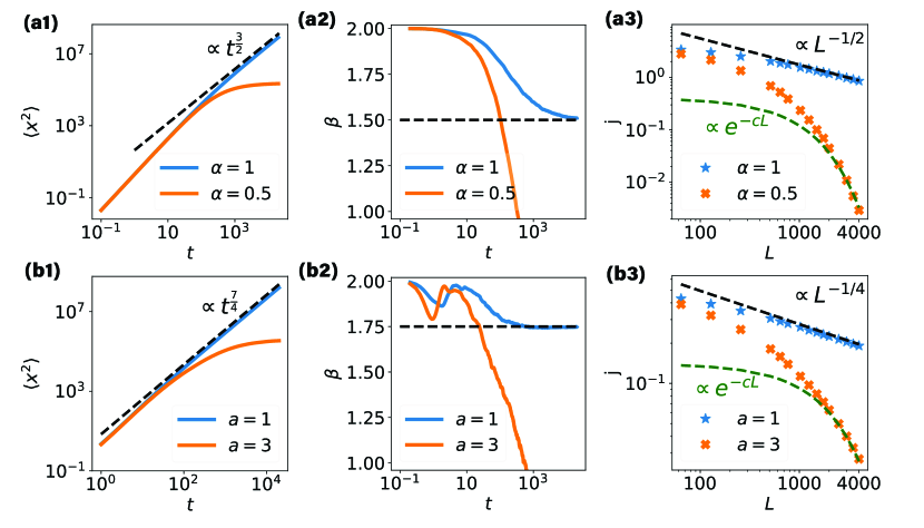
A single-particle state can be represented by $\Psi(t)=\sum_{x}\phi_{j}(t)\hat{c}_{j}^{\dagger}|0\rangle$. Since this model corresponds to a quadratic free fermion, we investigate its dynamic exponent $z$ through the evolution of the point initial state $\phi_{x}(t=0)=\delta_{0,j}$. Notably, the mean square displacement asymptotically grows as $\langle x^{2}\rangle\sim t^{2/z}$, where $\langle x^{2}\rangle(t)\equiv\sum_{j}j^{2}|\phi_{j}(t)|^{2}$.

For $\alpha=1$, the momentum distribution $|d_{k}|^{2}=(1+\alpha e^{i(\theta+k)})/\sqrt{1+|\alpha|^{2}}$ exhibits a nodal point at $k_{0}=\pi-\theta$ with order $n=1$. As long as $\theta$ is not 00 or $\pi$, which leads to $v(k_{0})=0$, the dynamical exponent would be the same. Without loss of generality, we set $\theta=\pi/2$. Numerical simulations indicate that the mean square displacement asymptotically grows as $\langle x^{2}\rangle\sim t^{3/2}$(Fig. 1(a1)(a2)) and the current under fixed boundary driven scales with system size as $j\sim L^{-1/2}$(Fig. 1(a3)), implying a dynamic exponent of $z=\frac{4}{3}$, characterizing the system as undergoing superdiffusion. Conversely, for $\alpha\neq 1$, such as $\alpha=0.5$, the momentum distribution exhibits no nodal points, resulting in the system behaving similarly to the Anderson model, indicating localization(Fig. 1(a1)(a3)). The details of the boundary-driven model setup are provided in Appendix B.

While the above discussion assumes that $\epsilon_{i}$ for every site $i$ is randomly and independently chosen to be $W$ with probability $p$, or 00 with a probability of $1-p$, our numerical simulations demonstrate that randomly choosing $\epsilon_{i}$ from the range $(-W/2,W/2)$ yields similar results (see Appendix C).

IV Time-reversal symmetry

Time-reversal symmetry plays a crucial role in shaping the dynamics of the system. Under this symmetry, the energy dispersion of $\hat{H}_{0}$ satisfies $E(k)=E(-k)$, and the momentum distribution of the impurity satisfies $d_{k}=d_{-k}^{*}$. In general, there always exists a momentum region $\bm{K}$ such that only $-k$ has the same energy as momentum $k$. In other word, when $k\in\bm{K}$, $E(k^{\prime})\neq E(k)$ unless $k^{\prime}=\pm k$.

Within this region $\bm{K}$, the reflection probability of a single impurity can be expressed as:

$$R_{1}(k)=c(k)|d_{k}|^{2}|d_{-k}|^{2}.$$ (16)

Moreover, if $d_{k_{0}}=0$, it implies $d_{-k_{0}}=0$. If $k_{0}\in\bm{K}$, this doubles the order of zeros of the reflection probability, leading to an enhanced divergent behavior of the localization length near node $k_{0}$:

$$\xi(k_{0}+q)=1/q^{4n}.$$ (17)

Consequently, the dynamical exponent is given by $z=\frac{8n}{8n-1}$, and $\langle x^{2}\rangle\sim t^{2-1/4n}$.

For a concrete example, consider a nearest-hopping model $H_{0}=\sum_{i}(\hat{c}_{i}^{\dagger}\hat{c}_{i+1}+\hat{c}_{i+1}^{\dagger}\hat{c}_{i})$ with 3-site time-reversal impurities $\hat{d}_{i}=(\hat{c}_{i-1}+a\hat{c}_{i}+\hat{c}_{i+1})/\sqrt{(2+a^{2})}$, where $a$ is a real number. The momentum distribution is given by $d_{k}=(2\cos k+a)/\sqrt{2+a^{2}}$. In this case, $\bm{K}=[-\pi,\pi]$.

For $|a|<2$, consider $a=1$, where $d_{k}$ has nodes with order $n=1$. Numerical simulations reveal that the nonequilibrium steady-state (NESS) current of this disordered chain under boundary-driven conditions scales with the system size as $j\sim L^{-1/4}$ (Fig. 1(b3)), and the mean square displacement grows as $\langle x^{2}\rangle\sim t^{7/4}$ at late times (Fig. 1(b1)(b2)).

In contrast, under condition $|a|>2$, for instance, we choose $a=3$. Here, $d_{k}$ exhibits no nodes. Numerical simulations indicate that the NESS current of this disorder chain under boundary-driven conditions decreases exponentially (Fig. 1(b3)), and the evolution of mean square displacement suggests system localization (Fig. 1(b1)).

V conclusion and discussion

In this paper, we present a new 1D disorder systems by replacing the onsite impurities in the Anderson model with nodal impurities. The nodal impurity model exhibits superdiffusive transport.

The mechanism driving superdiffusive transport is straightforward: on one hand, we have a free fermion model with ballistic eigenmodes. On the other hand, the scattering of nodal impurities localizes most eigenmodes except for the measure-zero eigenmodes with nodal momentum $k_{0}$. This leads to a power-law divergence of the localization length $\xi(k)$ at the node $k_{0}$. Modes with momenta near the nodes contribute to the superdiffusive transport, and the dynamical exponent $z$ is determined by the highest order $n$ of the node by $z=(4n-1)/4n$ in general. Furthermore, this superdiffusive behavior is enhanced under time-reversal symmetry, resulting in a dynamical exponent of $z=(8n-1)/8n$.

It’s crucial to note that the concept of “nodal points” is not limited to disorder systems; similar phenomena are observed in dephasing systems Wang et al. (2023). The underlying philosophy of this “nodal point” picture is both simple and general. A “nodal point” corresponds to a measure-zero ballistic mode, where the mean free path diverges. In cases where the divergent behavior near the nodal point $k_{0}$ follows a power law, modes in the vicinity of the nodal point have the potential to drive superdiffusive transport.

We believe that the “nodal point” picture can also be applied to construct superdiffusive models in interacting systems. For example, we can replace free fermion Hamiltonian $\hat{H}_{0}$ in our model with an integrable model, which also possesses ballistic modes. As long as we can find some local operator $O_{i}$, which can scatter these ballistic modes to diffusive or localized modes but leaves a specific mode with momentum $k_{0}$ unscattered, we can construct a superdiffusive model by using these operators as impurities, dephasing, or interactions. In this way, we may find a chaotic model exhibiting superdiffusive transport. We leave this for future study.

Acknowledgements.

Y.-P. W. thanks Marko Žnidarič for his valuable comments.

Appendix A Transmission probability with multiple impurities

In this appendix, following the demonstration of Müller and Delande (2010), we show that the averaged logarithm transmission probability of multiple impurities $\langle\log T\rangle$ is just the sum of logarithm transmission probability of single impurity when impurity density is low.

At first, we consider the scattering process of single impurity $V=\hat{d}^{\dagger}\hat{d}$, where $\hat{d}=\sum_{a=1}^{l}d_{a}\hat{c}_{a}$. We can decompose the wave function at the left ($L,x<0$) and right ($R,x>l$) into incoming and outgoing waves:

$\displaystyle\phi_{L}(x)=\phi^{in}_{L}e^{ikx}+\phi^{out}_{L}e^{ik^{\prime}x}$ (18)
$\displaystyle\phi_{R}(x)=\phi^{out}_{R}e^{ikx}+\phi^{in}_{R}e^{ik^{\prime}x}$ (19)

The outgoing amplitudes are linked to the incident amplitudes by the reflection and transmission coefficients $r$ and $t$ from the left, and $r^{\prime}$, $t^{\prime}$ from the right:

$\displaystyle\phi^{out}_{L}=t\phi^{in}_{L}+r^{\prime}\phi^{in}_{R}$ (20)
$\displaystyle\phi^{out}_{R}=r\phi^{in}_{L}+t^{\prime}\phi^{in}_{R}$ (21)

The scattering matrix can be defined as

$\displaystyle\begin{pmatrix}\phi_{L}^{out}\\ \phi_{R}^{out}\end{pmatrix}=S\begin{pmatrix}\phi_{L}^{in}\\ \phi_{R}^{in}\end{pmatrix}\quad\text{where}\ S=\begin{pmatrix}r&t^{\prime}\\ t&r^{\prime}\end{pmatrix}.$ (22)

The reflection and transmission probability from the left are respectively $R=|r|^{2}$ and $T=|t|^{2}$, and similar from the right $R^{\prime}=|r^{\prime}|^{2}$ and $T^{\prime}=|t^{\prime}|^{2}$. The probability flux conservation ensure that $S$ is unitary, $S^{\dagger}S=Id$, which leads to $T=T^{\prime}$, $R=R^{\prime}$ and $T+R=T^{\prime}+R^{\prime}=1$.

We can also decompose the wave function into left-moving and right-moving components:

$\displaystyle\phi_{L}(x)=\phi^{+}_{L}e^{ikx}+\phi^{-}_{L}e^{ik^{\prime}x}$ (23)
$\displaystyle\phi_{R}(x)=\phi^{+}_{R}e^{ikx}+\phi^{-}_{R}e^{ik^{\prime}x}$ (24)

The transfer matrix $M$ maps the the amplitudes from the left side of this impurity to the right:

$\displaystyle\begin{pmatrix}\phi_{R}^{+}\\ \phi_{R}^{-}\end{pmatrix}=M\begin{pmatrix}\phi_{L}^{+}\\ \phi_{L}^{-}\end{pmatrix}$ (25)

From equation (22), we can get the transfer matrix

$\displaystyle M=\begin{pmatrix}t-rr^{\prime}/t^{\prime}&r^{\prime}/t^{\prime}\\ -r/t&1/t\end{pmatrix}.$ (26)

In multiple impurities case, the total transfer matrix is just the product of transfer matrixes of all impurities. In two impurity case, $M_{12}=M_{1}M_{2}$. The total transmission amplitude is

$$t_{12}=\frac{t_{1}t_{2}}{1-r_{1}^{\prime}r_{2}}$$ (27)

The logarithm transmission probability is

$\displaystyle\log T_{12}=\log T_{1}+\log T_{2}+\log|1-\sqrt{R_{1}R_{2}}e^{i\theta}|$ (28)

When distance $\delta x$ between two impurities is randomly and $k\delta x\gg 2\pi$, $\theta$ is also randomly distributed in $[0,2\pi]$.

$$\langle\log|1-\sqrt{R_{1}R_{2}}e^{i\theta}|\rangle=\int_{0}^{2\pi}d\theta\log|1-\sqrt{R_{1}R_{2}}e^{i\theta}|=0$$ (29)

Thus, the log-averaged transmission is additive

$$\langle\log T_{12}\rangle=\log T_{1}+\log T_{2}$$ (30)

Considering that $\epsilon_{i}$ in inpurity model (Eq. 31) for every site $i$ is randomly and independently chosen to be $W$ with probability $p$, or 00 with a probability of $1-p$.

$\displaystyle\hat{H}$ $\displaystyle=\sum_{k}E_{k}\hat{c}_{k}^{\dagger}\hat{c}_{k}+\sum_{i}\epsilon_{i}\hat{d}_{i}^{\dagger}\hat{d}_{i}$ (31)

There are average $pL$ impurities in this disorder chain. Under the condition $k/p\gg 2\pi$, the log-averaged transmission probability satisfies

$$\langle\log T(k)\rangle=pL\log T_{1}(k)$$ (32)

Furthermore, Müller and Delande (2010) illustrate that the typical transmission is $T_{typ}=\exp\{\langle\log T\rangle\}$. Therefore, we define localization length as $\xi(k)=-1/(pL\log T_{1}(k))$.

Appendix B Boundary driven setup

In this appendix, we illustrate the boundary driven setup utilized to derive the scaling relation between NESS current and system size, a method commonly employed to investigate transport properties in various studiesŽnidarič (2011); Žnidarič et al. (2016); Žnidarič (2020); Varma et al. (2017b).

We couple the first and the last site to baths described phenomenologically by the following 4 Lindblad operators,

$\displaystyle\mathcal{L}^{(\text{bath})}(\rho)=\sum_{k=1}^{4}2L_{k}\rho L_{k}^{\dagger}$ $\displaystyle-\rho L_{k}^{\dagger}L_{k}-L_{k}^{\dagger}L_{k}\rho$ (33)
$\displaystyle L_{1}=\sqrt{\Gamma(1+\mu)}\hat{c}^{\dagger}_{1},\quad$ $\displaystyle L_{2}=\sqrt{\Gamma(1-\mu)}\hat{c}_{1}$ (34)
$\displaystyle L_{3}=\sqrt{\Gamma(1-\mu)}\hat{c}^{\dagger}_{L},\quad$ $\displaystyle L_{4}=\sqrt{\Gamma(1+\mu)}\hat{c}_{L}$ (35)

where $\rho$ is density matrix. The density matrix’s evolution is governed by the Lindblad master equation:

$$\frac{\mathrm{d}\rho}{\mathrm{d}t}=\mathrm{i}[\rho,\hat{H}]+\mathcal{L}^{(\text{bath})}(\rho).$$ (36)

Here, $\hat{H}=\sum_{i}(\hat{c}_{i}^{\dagger}\hat{c}_{i+1}+\hat{c}_{i+1}^{\dagger}\hat{c}_{i})+\sum_{i}\epsilon_{i}\hat{d}_{i}^{\dagger}\hat{d}_{i}=\sum_{ij}H_{ij}\hat{c}^{\dagger}_{i}\hat{c}_{j}$ represents the Hamiltonian of the impurity model. In free fermion case, current $j$ is proportional to $\mu$. Without loss of generality, we set $\Gamma=\mu=1$. As the complete Liouvillean is quadratic, the equation of motion is closed, and the NESS is specified by the two-point green function $C$, where $C_{ij}=\langle\hat{c}^{\dagger}_{i}\hat{c}_{j}\rangle=\operatorname{Tr}(\hat{c}^{\dagger}_{i}\hat{c}_{j}\rho)$.

Since the density matrix satisfies the Lindblad master equation (36), in the Heisenberg picture, the evolution of an operator $\hat{O}$ satisfies:

$\displaystyle\frac{\mathrm{d}\hat{O}}{\mathrm{d}t}$ $\displaystyle=i[\hat{H},\hat{O}]+\sum_{k}2L_{k}^{\dagger}\hat{O}L_{k}-\hat{O}L^{\dagger}_{k}L_{k}-L^{\dagger}_{k}L_{k}\hat{O}$ (37)
$\displaystyle=i[\hat{H},\hat{O}]+\sum_{k}L_{k}^{\dagger}[\hat{O},L_{k}]+[L^{\dagger}_{k},\hat{O}]L_{k}.$ (38)

By substituting $\hat{O}=\hat{c}^{\dagger}_{i}\hat{c}_{j}$ into Eq. (37), we obtain the evolution of the two-point green function:

$$\frac{\mathrm{d}C}{\mathrm{d}t}=XC+CX^{\dagger}+P,$$ (39)

where $X=iH^{T}-R$, $R_{11}=R_{LL}=1$, $P_{11}=2$, and all other elements of $R$ and $P$ is zero.

The current of $\hat{H}_{0}=\sum_{i}(\hat{c}_{i}^{\dagger}\hat{c}_{i+1}+\hat{c}_{i+1}^{\dagger}\hat{c}_{i})$ is

$\displaystyle j=\langle\hat{c}_{i}^{\dagger}\hat{c}_{i+1}-\hat{c}_{i+1}^{\dagger}\hat{c}_{i}\rangle=2\operatorname{Im}C_{i,i+1}.$ (40)

Considering the case of an l-site disorder $\hat{d}_{i}=\sum_{a=0}^{l-1}d_{a}\hat{c}_{i+a}$, we let $\epsilon_{1}=\epsilon_{2}=0$, ensuring no disorder hopping between sites $1$ and $2$. Consequently, the NESS current of the disorder chain is $j=2\operatorname{Im}C_{1,2}$.

Appendix C Numerical results for sampling $\epsilon_{i}$ from uniform distribution

In this section, we present numerical simulations (Fig. 2) for the case that disorder strength $\epsilon_{i}$ is randomly and independently sampled from $[-W/2,W/2]$. The physical quantity is the same as Fig. 1 in main text.

Refer to caption
Figure 2: Numerical results of nodal impurity models: (a1)(a2)(a3) for 2-site inpurity $\hat{d}_{i}=(\hat{c}_{i}+i\alpha\hat{c}_{i+1})/\sqrt{1+|\alpha|^{2}}$, and (b1)(b2)(b3) for 3-site time-reversal impurity $\hat{d}_{i}=(\hat{c}_{i-1}+a\hat{c}_{i}+\hat{c}_{i+1})/\sqrt{2+a^{2}}$. (a1) Evolution of mean-square displacement in 2-site impurity model: Numerical simulations depict the evolution of mean-square displacement in 2-site impurity model $\hat{d}_{i}=(\hat{c}_{i}+\alpha i\hat{c}_{i+1})/\sqrt{1+|\alpha|^{2}}$, showcasing nodal impurity with $\alpha=1$ (blue line) and non-nodal impurity with $\alpha=0.5$ (orange line). The initial state is $\psi(x)=\delta_{0,x}$. The impurity chain with nodal impurities exhibits superdiffusive transport, characterized by an asymptotic behavior of $\langle x^{2}\rangle\sim t^{3/2}$ (black dashed line), while the non-nodal impurity model displays localized behavior. (b1) Evolution of mean-square displacement in 3-site disorder model: The same for 3-site impurity $\hat{d}_{i}=(\hat{c}_{i-1}+a\hat{c}_{i}+\hat{c}_{i+1})/\sqrt{2+a^{2}}$. Blue line represents the nodal case $a=1$, and the orange line represents the non-nodal case $a=3$. (a2) Exponent evolution in 2-site impurity model: Depicts the evolution of the exponent $\beta(t)=\frac{d\log\langle x^{2}\rangle(t)}{d\log t}$ for the model with 2-site impurity $\hat{d}_{i}=(\hat{c}_{i}+i\hat{c}_{i+1})/\sqrt{2}$. The behavior of $\beta(t)$ converges to $3/2$ at long times. (b2) Exponent evolution in 3-site impurity model: Depicts the evolution of the same exponent for the model with 3-site disorder $\hat{d}_{i}=(\hat{c}_{i-1}+\hat{c}_{i}+\hat{c}_{i+1})/\sqrt{3}$. The behavior of $\beta(t)$ converges to $7/4$ at long times. (a3) NESS current in 2-site impurity model: NESS current of a boundary-driven quasi-particle disorder chain with 2-site impurity $\hat{d}_{i}=\hat{c}_{i}+\alpha i\hat{c}_{i+1}$, featuring nodal impurities with $\alpha=1$ (blue line) and non-nodal impurities with $\alpha=0.5$ (orange line). The current of the nodal disorder chain decreases as $j\sim L^{-1/2}$, whereas the non-nodal disorder chain exhibits exponential decay. (b3) NESS current in 3-site impurity model: The same for 3-site impurity $\hat{d}_{i}=(\hat{c}_{i-1}+a\hat{c}_{i}+\hat{c}_{i+1})/\sqrt{2+a^{2}}$. The blue line represents the nodal case $a=1$, whose current decreases as $j\sim L^{-1/4}$. The orange line represents the non-nodal case $a=3$, whose current decreases exponentially. In all the figures, the disorder strength is $W=1$, and $\epsilon_{i}$ for every site $i$ is randomly and independently sampling from $[-W/2,W/2]$. All the data is averaged over 200 random disorder configurations.

References

  • Bertini et al. (2021) B. Bertini, F. Heidrich-Meisner, C. Karrasch, T. Prosen, R. Steinigeweg,  and M. Žnidarič, “Finite-temperature transport in one-dimensional quantum lattice models,” Rev. Mod. Phys. 93, 025003 (2021).
  • Sirker (2020) Jesko Sirker, “Transport in one-dimensional integrable quantum systems,” SciPost Phys. Lect. Notes , 17 (2020).
  • Medenjak et al. (2017) Marko Medenjak, Katja Klobas,  and Toma ž Prosen, “Diffusion in deterministic interacting lattice systems,” Phys. Rev. Lett. 119, 110603 (2017).
  • Dhar (2008) Abhishek Dhar, “Heat transport in low-dimensional systems,” Advances in Physics 57, 457–537 (2008)https://doi.org/10.1080/00018730802538522 .
  • Cipriani et al. (2005) P. Cipriani, S. Denisov,  and A. Politi, “From anomalous energy diffusion to levy walks and heat conductivity in one-dimensional systems,” Phys. Rev. Lett. 94, 244301 (2005).
  • Chen et al. (2014) Shunda Chen, Jiao Wang, Giulio Casati,  and Giuliano Benenti, “Nonintegrability and the fourier heat conduction law,” Phys. Rev. E 90, 032134 (2014).
  • Nahum et al. (2017) Adam Nahum, Jonathan Ruhman, Sagar Vijay,  and Jeongwan Haah, “Quantum entanglement growth under random unitary dynamics,” Phys. Rev. X 7, 031016 (2017).
  • Nahum et al. (2018) Adam Nahum, Sagar Vijay,  and Jeongwan Haah, “Operator spreading in random unitary circuits,” Phys. Rev. X 8, 021014 (2018).
  • Rakovszky et al. (2018) Tibor Rakovszky, Frank Pollmann,  and C. W. von Keyserlingk, “Diffusive hydrodynamics of out-of-time-ordered correlators with charge conservation,” Phys. Rev. X 8, 031058 (2018).
  • Khemani et al. (2018) Vedika Khemani, Ashvin Vishwanath,  and David A. Huse, “Operator spreading and the emergence of dissipative hydrodynamics under unitary evolution with conservation laws,” Phys. Rev. X 8, 031057 (2018).
  • von Keyserlingk et al. (2018) C. W. von Keyserlingk, Tibor Rakovszky, Frank Pollmann,  and S. L. Sondhi, “Operator hydrodynamics, otocs, and entanglement growth in systems without conservation laws,” Phys. Rev. X 8, 021013 (2018).
  • Zhou et al. (2020a) Tianci Zhou, Shenglong Xu, Xiao Chen, Andrew Guo,  and Brian Swingle, “Operator lévy flight: Light cones in chaotic long-range interacting systems,” Phys. Rev. Lett. 124, 180601 (2020a).
  • Anderson (1958) P. W. Anderson, “Absence of diffusion in certain random lattices,” Phys. Rev. 109, 1492–1505 (1958).
  • Thouless (1972) D J Thouless, “A relation between the density of states and range of localization for one dimensional random systems,” Journal of Physics C: Solid State Physics 5, 77 (1972).
  • Hirota and Ishii (1971) Tōru Hirota and Kazushige Ishii, “Exactly soluble models of one-dimensional disordered systems,” Progress of Theoretical Physics 45, 1713–1715 (1971).
  • Bulchandani et al. (2021) Vir B Bulchandani, Sarang Gopalakrishnan,  and Enej Ilievski, “Superdiffusion in spin chains,” Journal of Statistical Mechanics: Theory and Experiment 2021, 084001 (2021).
  • Dunlap et al. (1990) David H. Dunlap, H-L. Wu,  and Philip W. Phillips, “Absence of localization in a random-dimer model,” Phys. Rev. Lett. 65, 88–91 (1990).
  • Ostlund et al. (1983) Stellan Ostlund, Rahul Pandit, David Rand, Hans Joachim Schellnhuber,  and Eric D. Siggia, “One-dimensional schrödinger equation with an almost periodic potential,” Phys. Rev. Lett. 50, 1873–1876 (1983).
  • Kohmoto et al. (1983) Mahito Kohmoto, Leo P. Kadanoff,  and Chao Tang, “Localization problem in one dimension: Mapping and escape,” Phys. Rev. Lett. 50, 1870–1872 (1983).
  • Hiramoto and Abe (1988) Hisashi Hiramoto and Shuji Abe, “Dynamics of an electron in quasiperiodic systems. i. fibonacci model,” Journal of the Physical Society of Japan 57, 230–240 (1988).
  • Žnidarič (2011) Marko Žnidarič, “Spin transport in a one-dimensional anisotropic heisenberg model,” Phys. Rev. Lett. 106, 220601 (2011).
  • Ljubotina et al. (2017) Marko Ljubotina, Marko Žnidarič,  and Tomaž Prosen, “Spin diffusion from an inhomogeneous quench in an integrable system,” Nature Communications 8, 16117 (2017).
  • Ljubotina et al. (2019) Marko Ljubotina, Marko Žnidarič,  and Toma ž Prosen, “Kardar-parisi-zhang physics in the quantum heisenberg magnet,” Phys. Rev. Lett. 122, 210602 (2019).
  • Castro-Alvaredo et al. (2016) Olalla A. Castro-Alvaredo, Benjamin Doyon,  and Takato Yoshimura, “Emergent hydrodynamics in integrable quantum systems out of equilibrium,” Phys. Rev. X 6, 041065 (2016).
  • Bertini et al. (2016) Bruno Bertini, Mario Collura, Jacopo De Nardis,  and Maurizio Fagotti, “Transport in out-of-equilibrium $xxz$ chains: Exact profiles of charges and currents,” Phys. Rev. Lett. 117, 207201 (2016).
  • Gopalakrishnan and Vasseur (2019) Sarang Gopalakrishnan and Romain Vasseur, “Kinetic theory of spin diffusion and superdiffusion in $xxz$ spin chains,” Phys. Rev. Lett. 122, 127202 (2019).
  • Claeys et al. (2022) Pieter W. Claeys, Austen Lamacraft,  and Jonah Herzog-Arbeitman, “Absence of superdiffusion in certain random spin models,” Phys. Rev. Lett. 128, 246603 (2022).
  • De Nardis et al. (2021) Jacopo De Nardis, Sarang Gopalakrishnan, Romain Vasseur,  and Brayden Ware, “Stability of superdiffusion in nearly integrable spin chains,” Phys. Rev. Lett. 127, 057201 (2021).
  • Friedman et al. (2020) Aaron J. Friedman, Sarang Gopalakrishnan,  and Romain Vasseur, “Diffusive hydrodynamics from integrability breaking,” Phys. Rev. B 101, 180302 (2020).
  • Ilievski et al. (2021) Enej Ilievski, Jacopo De Nardis, Sarang Gopalakrishnan, Romain Vasseur,  and Brayden Ware, “Superuniversality of superdiffusion,” Phys. Rev. X 11, 031023 (2021).
  • Ye et al. (2022) Bingtian Ye, Francisco Machado, Jack Kemp, Ross B. Hutson,  and Norman Y. Yao, “Universal kardar-parisi-zhang dynamics in integrable quantum systems,” Phys. Rev. Lett. 129, 230602 (2022).
  • Mirlin et al. (1996) Alexander D. Mirlin, Yan V. Fyodorov, Frank-Michael Dittes, Javier Quezada,  and Thomas H. Seligman, “Transition from localized to extended eigenstates in the ensemble of power-law random banded matrices,” Phys. Rev. E 54, 3221–3230 (1996).
  • Borland and Menchero (1999) Lisa Borland and JG Menchero, “Nonextensive effects in tight-binding systems with long-range hopping,” Brazilian journal of physics 29, 169–178 (1999).
  • Varma et al. (2017a) Vipin Kerala Varma, Clélia de Mulatier,  and Marko Žnidarič, “Fractality in nonequilibrium steady states of quasiperiodic systems,” Phys. Rev. E 96, 032130 (2017a).
  • Saha et al. (2019) Madhumita Saha, Santanu K. Maiti,  and Archak Purkayastha, “Anomalous transport through algebraically localized states in one dimension,” Phys. Rev. B 100, 174201 (2019).
  • Richter et al. (2023) Jonas Richter, Oliver Lunt,  and Arijeet Pal, “Transport and entanglement growth in long-range random clifford circuits,” Phys. Rev. Res. 5, L012031 (2023).
  • Zhou et al. (2020b) Tianci Zhou, Shenglong Xu, Xiao Chen, Andrew Guo,  and Brian Swingle, “Operator lévy flight: Light cones in chaotic long-range interacting systems,” Phys. Rev. Lett. 124, 180601 (2020b).
  • Wang et al. (2023) Yu-Peng Wang, Chen Fang,  and Jie Ren, “Superdiffusive transport in quasi-particle dephasing models,” arXiv preprint arXiv:2310.03069  (2023).
  • Esposito and Gaspard (2005) Massimiliano Esposito and Pierre Gaspard, “Exactly solvable model of quantum diffusion,” Journal of statistical physics 121, 463–496 (2005).
  • Žnidarič (2010) Marko Žnidarič, “Exact solution for a diffusive nonequilibrium steady state of an open quantum chain,” Journal of Statistical Mechanics: Theory and Experiment 2010, L05002 (2010).
  • Cao et al. (2019) Xiangyu Cao, Antoine Tilloy,  and Andrea De Luca, “Entanglement in a fermion chain under continuous monitoring,” SciPost Phys. 7, 024 (2019).
  • Sakurai and Napolitano (2020) J.J. Sakurai and J. Napolitano, Modern Quantum Mechanics (Cambridge University Press, 2020).
  • Jin et al. (2020) Tony Jin, Michele Filippone,  and Thierry Giamarchi, “Generic transport formula for a system driven by markovian reservoirs,” Phys. Rev. B 102, 205131 (2020).
  • Žnidarič et al. (2016) Marko Žnidarič, Antonello Scardicchio,  and Vipin Kerala Varma, “Diffusive and subdiffusive spin transport in the ergodic phase of a many-body localizable system,” Phys. Rev. Lett. 117, 040601 (2016).
  • Landi et al. (2022) Gabriel T. Landi, Dario Poletti,  and Gernot Schaller, “Nonequilibrium boundary-driven quantum systems: Models, methods, and properties,” Rev. Mod. Phys. 94, 045006 (2022).
  • Müller and Delande (2010) Cord A Müller and Dominique Delande, “Disorder and interference: localization phenomena,” arXiv preprint arXiv:1005.0915  (2010).
  • Žnidarič (2020) Marko Žnidarič, “Weak integrability breaking: Chaos with integrability signature in coherent diffusion,” Phys. Rev. Lett. 125, 180605 (2020).
  • Varma et al. (2017b) Vipin Kerala Varma, Clélia de Mulatier,  and Marko Žnidarič, “Fractality in nonequilibrium steady states of quasiperiodic systems,” Phys. Rev. E 96, 032130 (2017b).