mlr3summary: Concise and interpretable summaries for machine learning models

Susanne Dandl, Marc Becker, Bernd Bischl, Giuseppe Casalicchio, Ludwig Bothmann mlr3summary: Concise and interpretable summaries for machine learning models mlr3summary: Concise and interpretable summaries for machine learning models This work introduces a novel R package for concise, informative summaries of machine learning models. We take inspiration from the summary function for (generalized) linear models in R, but extend it in several directions: First, our summary function is model-agnostic and provides a unified summary output also for non-parametric machine learning models; Second, the summary output is more extensive and customizable – it comprises information on the dataset, model performance, model complexity, model’s estimated feature importances, feature effects, and fairness metrics; Third, models are evaluated based on resampling strategies for unbiased estimates of model performances, feature importances, etc. Overall, the clear, structured output should help to enhance and expedite the model selection process, making it a helpful tool for practitioners and researchers alike. Model summary, interpretable machine learning, resampling-based evaluation Model summary, interpretable machine learning, resampling-based evaluation Ludwig Bothmann
Institut für Statistik
Ludwig-Maximilians-Universität München, Germany
Ludwigstr. 33, 80539 Munich, Germany
Munich Center for Machine Learning (MCML), Germany
E-mail:

1 Introduction

Machine learning (ML) increasingly supports decision-making processes in various domains. A data scientist has a wide range of models available, ranging from intrinsically interpretable models such as linear models to highly complex models such as random forests or gradient boosted trees. Intrinsically interpretable models can come at the expense of generalization performance, i.e., the model’s capability to predict accurately on future data. Being able to interpret predictive models is either often a strict requirement for scientific inference or at least a very desirable property to audit models in other (more technical) contexts. Many methods have been proposed for interpreting black-box ML models in the field of interpretable ML (IML).

For comparing (generalized) linear models (GLMs), the stats package in R offers a summary function, which only requires the model (fitted with lm or glm) as input. As an example, glm is applied to a preprocessed version of the German credit dataset (Hofmann, 1994) (available in the package via data("credit", package = "mlr3summary")):

⬇

> logreg = glm(risk ~., data = credit,

+ family = binomial(link = "logit"))

> summary(logreg)

¯Call:
¯glm(formula = risk ~., data = credit, family = binomial(link = "logit"))
¯Coefficients:
¯Estimate Std. Error z value Pr(>|z|)
¯(Intercept)        1.057e+00  3.646e-01   2.900  0.00373 **
¯age                9.103e-03  8.239e-03   1.105  0.26925
¯...
¯Residual deviance: 656.19  on 515  degrees of freedom
¯AIC: 670.19
¯...

This (shortened) summary informs about the significance of variables (Pr(>|z|)), their respective effect size and direction (Estimate), as well as the goodness-of-fit of the model (Residual deviance and AIC). Unfortunately, many other non-parametric ML models currently cannot be analyzed similarly: either targeted implementations exist for specific model classes, or an array of different model-agnostic interpretability techniques (e.g., to derive feature importance) scattered across multiple packages (Molnar et al., 2018; Biecek, 2018; Zargari Marandi, 2023) must be employed. However, especially in applied data science, a user often performs model selection or model comparison across an often diverse pool of candidate models, so a standardized diagnostic output becomes highly desirable.

Another issue is that in the glm-based summary, the goodness-of-fit is only evaluated on the training data, but not on hold-out/test data. While this might be appropriate for GLM-type models – provided proper model diagnosis has been performed – this is not advisable for non-parametric and non-linear models, which can overfit the training data. Here, hold-out test data or in general resampling techniques like cross-validation should be used for proper estimation of the generalization performance Simon (2007). Such resampling-based performance estimation should also be used for loss-based IML methods. For interpretability methods that only rely on predictions, this might also be advisable but might not lead to huge differences in results (Molnar et al., 2022, 2023).

Contributions

With the mlr3summary package, we provide a novel model-agnostic summary function for ML models and learning algorithms in R. This is facilitated by building upon mlr3 (Lang et al., 2019; Bischl et al., 2024) – a package ecosystem for applied ML, including resampling-based performance assessment. The summary function returns a structured overview that gives information on the underlying dataset and model, generalization performances, complexity of the model, fairness metrics, and feature importances and effects. For the latter two, the function relies on model-agnostic methods from the field of IML. The output is customizable via a flexible control argument to allow adaptation to different application scenarios. The mlr3summary package is released under LGPL-3 on GitHub (https://github.com/mlr-org/mlr3summary) and CRAN (https://cran.r-project.org/package=mlr3summary). Documentations in the form of help pages are available as well as unit tests. The example code of this manuscript is available via demo("credit", package = "mlr3summary").

2 Related work

Most R packages that offer model summaries are restricted to parametric models and extend the stats summary method (e.g., modelsummary (Arel-Bundock, 2022), broom (Robinson et al., 2023)). Performance is only assessed based on training data – generalization errors are not provided. Packages that can handle diverse ML models focus primarily on performance assessment (e.g., mlr3 (Lang et al., 2019), caret (Kuhn and Max, 2008)). Packages that primarily consider feature importances and effects do not provide overviews in a concise, decluttered format but provide extensive reports (e.g., modelDown (Romaszko et al., 2019) and modelStudio (Baniecki and Biecek, 2019) based on DALEX (Biecek, 2018), or explainer (Zargari Marandi, 2023)). While it is possible to base the assessment on hold-out/test data, assessment based on resampling is not automatically supported by these packages. Overall, to the best of our knowledge, there is no R package yet that allows for a concise yet informative overview based on resampling-based performance assessment, model complexity, feature importance and effect directions, and fairness metrics.

3 Design, functionality, and example

The core function of the mlr3summary package is the S3-based summary function for mlr3 Learner objects. It has three arguments: object reflects a trained model – a model of class Learner fitted with mlr3; resample_result reflects the results of resampling – a ResampleResult object fitted with mlr3; control reflects some control arguments – a list created with summary_control (details in Section 3.2).

The mlr3 package is the basis of mlr3summary because it provides a unified interface to diverse ML models and resampling strategies. A general overview of the mlr3 ecosystem is given in Bischl et al. (Bischl et al., 2024). With mlr3, the modelling process involves the following steps: (1) initialize a regression or classification task, (2) choose a regression or classification learner, (3) train a model with the specified learner on the initialized task, (4) apply a resampling strategy. The last step is necessary to receive valid estimates for performances, importances, etc., as mentioned in Section 1. The following lines of code illustrate steps (1)-(4) on the (preprocessed) credit dataset from Section 1 using a ranger random forest. As a resampling strategy, we conduct $3$-fold cross-validation.

⬇

> task = TaskClassif$new(id = "credit", backend = credit,

+ target = "risk")

> rf = lrn("classif.ranger", predict_type = "prob")

> rf$train(task)

> cv3 = rsmp("cv", folds = 3L)

> rr = resample(task = task, learner = rf, resampling = cv3,

+ store_models = TRUE)

Internally, the resample function fits, in each iteration, the model on the respective training data, uses the model to predict the held-out test data, and stores the predictions in the result object. To compute performances, complexities, importances, and other metrics, the summary function iteratively accesses the models and datasets within the resulting resample object, which requires setting the parameter store_models = TRUE within the resample function. For the final summary output, the results of each iteration are aggregated (e.g., averages and standard deviations (sds)).

3.1 Summary function and output

This section shows the summary call and output for the random forest of the previous credit example and provides some details on each displayed paragraph.

⬇

> summary(object = rf, resample_result = rr)

General provides an overview of the task, the learner (including its hyperparameters), and the resampling strategy.

Residuals display the distribution of residuals of hold-out data over the resampling iterations. For regression models, the residuals display the difference between true and predicted outcome. For classifiers that return class probabilities, the residuals are defined as the difference between predicted probabilities and a one-hot-encoding of the true class. For classifiers that return classes, a confusion matrix is shown.

Performance displays averages and sds (in $[\,]$) of performance measures over the iterations. The shown performance values are the area-under-the-curve (auc), the F-score (fbeta), the binary Brier score (bbrier), and Mathew’s correlation coefficient (mcc).

The arrows display whether lower or higher values refer to a better performance. “(macro)” indicates a macro aggregation, i.e., measures are computed for each iteration separately before averaging. “(micro)” would indicate that measures are computed across all iterations (see Bischl et al. (2024) for details).

Complexity displays averages and sds of two model complexity measures proposed by Molnar et al. (Molnar et al., 2020): sparsity shows the number of used features that have a non-zero effect on the prediction (evaluated by accumulated local effects (ale) (Apley and Zhu, 2020)); interaction_strength shows the scaled approximation error between a main effect model (based on ale) and the prediction function.

Importance shows the averages and sds of feature importances over the iterations. The first column (pdp) displays importances based on the sds of partial dependence curves (Friedman, 2001; Greenwell et al., 2018), the second column (pfi.ce) shows the results for permutation feature importance Breiman (2001); Fisher et al. (2019).

Effects shows average effect plots over the iterations – partial dependence plots (pdp) and ale plots (Friedman, 2001; Apley and Zhu, 2020). For binary classifiers, the effect plots are only shown for the positively-labeled class (here, task$positive = "good"). For multi-class classifiers, the effect plots are given for each outcome class separately (one vs. all). For categorical features, the bars are ordered according to the factor levels of the feature.

The learner can also be a complete pipeline from mlr3pipelines (Binder et al., 2021), where the most common case would be an ML model with associated pre-processing steps. Then, the summary output also shows some basic information about the pipeline. Since preprocessing steps are treated as being part of the learner, the summary output is displayed on the original data (e.g., despite one-hot encoding of categorical features, importance results are not shown for each encoding level separately). The learner can also be an AutoTuner from mlr3tuning, where automatic processes for tuning the hyperparameters are conducted. Examples on pipelining and tuning are given in the demo of the package.

3.2 Customizations

The output of the summary function can be customized via a control argument which requires a list created with the function summary_control as an input. If no control is specified, the following default setting is used:

⬇

> summary_control(measures = NULL,

+ complexity_measures = c("sparsity", "interaction_strength"),

+ importance_measures = NULL, n_important = 15L,

+ effect_measures = c("pdp", "ale"),

+ fairness_measures = NULL, protected_attribute = NULL,

+ hide = NULL, digits = max(3L, getOption("digits") - 3L))

Performances are adaptable via measures, complexities via complexity_measures, importances via importance_measures and effects via effect_measures within summary_control. Examples are given in the demo of the package. The default for measures and importance_ measures is NULL, which results in a collection of commonly reported measures being chosen, based on the task type – for concrete measures see the help page (?summary_control). n_important reflects that, by default, only the $15$ most important features are displayed in the output. This is especially handy for high-dimensional data. With hide, paragraphs of the summary output can be omitted (e.g., "performance") and with digits, the number of printed digits is specified.

Fairness assessment for classification and regression models is also available in mlr3summary based on the mlr3fairness package (Pfisterer et al., 2023). Therefore, a protected attribute must be specified. This can be done either within the task by updating the feature roles or by specifying a protected_attribute in summary_control. The following shows the code and output when specifying sex as a protected attribute. The shown default fairness measures are demographic parity (dp), conditional use accuracy equality (cuae) and equalized odds (eod), other measures are possible via fairness_measures in summary_control.

⬇

> summary(object = rf, resample_result = rr,

+ control = summary_control(protected_attribute = "sex"))

4 Runtime assessment

To assess how the runtime scales with differing numbers of features $p\in\{5,10,25,50,100\}$ and numbers of observations $n\in\{50,100,500,1000,2000\}$, we conducted a simulation study. Given $X_{1},X_{2},X_{3}\sim U(0,1)$, $X_{4}\sim Bern(0.75)$, the data generating process is $y=f(\mathbf{x})+\epsilon$ with $f(\mathbf{x})=4x_{1}+4x_{2}+4x_{4}x_{3}^{2}$ and $\epsilon\sim N(0,0.1\cdot f(\mathbf{x}))$. As noise variables, $X_{5}$ as a categorical feature with five classes, and $X_{6},...,X_{p}\sim N(0,1)$ were added to the data. We trained random forests and linear main effect models on the datasets and conducted 3-fold cross-validation. The first two figures in Figure 1 show that runtimes of the linear model were lower compared to the random forest. To improve runtimes, we added parallelization over the resampling iterations (via the future package (Bengtsson, 2021)) as another feature to mlr3summary – results for the random forest (with $3$ cores) are on the right. Overall, scaling of runtimes is worse in $p$ than in $n$.

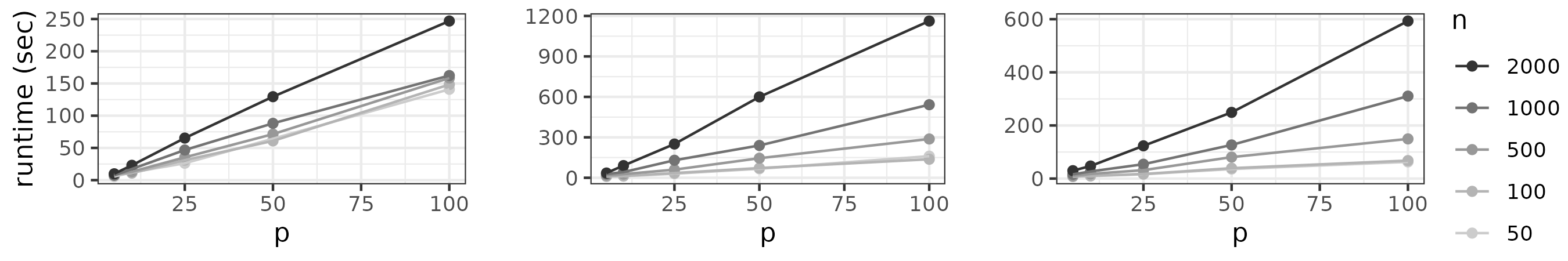
Figure 1: Runtimes of the summary function for linear models (left), and random forests without (middle) and with (right) parallelization, for differing numbers of features $p$ and observations $n$.

5 Outlook and discussion

In conclusion, this paper introduces a novel R package for concise model summaries. The summary output is highly adaptable due to a control argument and might be extended in the future. We also plan to offer a report function for detailed visualizations and model comparisons. To assess importance and effects of single features, mlr3summary builds upon the iml and fastshap packages. These packages only offer a limited set of interpretation methods. Recommended alternatives to permutation feature importances like conditional feature importance Molnar et al. (2022), are currently not available in a proper R package (published on CRAN). Our summary also currently lacks proper statistical tests for importances or confidence intervals for performances. This is because unbiased estimates of the variance are required which is a challenge for resampling strategies and the available methods that propose unbiased estimates are computationally infeasible (e.g., due to many model refits) (Molnar et al., 2023; Stephen Bates and Tibshirani, 2023). Addressing this issue requires some concerted efforts from the research community. If methods are readily available in R, we are happy to integrate them in mlr3summary.

References

- Apley and Zhu (2020) Apley DW, Zhu J (2020). “Visualizing the Effects of Predictor Variables in Black Box Supervised Learning Models.” Journal of the Royal Statistical Society Series B: Statistical Methodology, 82(4), 1059–1086. 10.1111/rssb.12377.
- Arel-Bundock (2022) Arel-Bundock V (2022). “modelsummary: Data and Model Summaries in R.” Journal of Statistical Software, 103(1), 1–23. 10.18637/jss.v103.i01.
- Baniecki and Biecek (2019) Baniecki H, Biecek P (2019). “modelStudio: Interactive Studio with Explanations for ML Predictive Models.” Journal of Open Source Software, 4(43), 1798. 10.21105/joss.01798.
- Bengtsson (2021) Bengtsson H (2021). “A Unifying Framework for Parallel and Distributed Processing in R using Futures.” The R Journal, 13(2), 208–227. 10.32614/RJ-2021-048.
- Biecek (2018) Biecek P (2018). “DALEX: Explainers for Complex Predictive Models in R.” Journal of Machine Learning Research, 19(84), 1–5.
- Binder et al. (2021) Binder M, Pfisterer F, Lang M, Schneider L, Kotthoff L, Bischl B (2021). “mlr3pipelines - Flexible Machine Learning Pipelines in R.” Journal of Machine Learning Research, 22(184), 1–7.
- Bischl et al. (2024) Bischl B, Sonabend R, Kotthoff L, Lang M (2024). Applied machine learning using mlr3 in R. Chapman and Hall/CRC. ISBN 9781003402848. 10.1201/9781003402848.
- Breiman (2001) Breiman L (2001). “Random Forests.” Machine Learning, 45(1), 5–32. ISSN 0885-6125. 10.1023/a:1010933404324.
- Fisher et al. (2019) Fisher A, Rudin C, Dominici F (2019). “All Models are Wrong, but Many are Useful: Learning a Variable’s Importance by Studying an Entire Class of Prediction Models Simultaneously.” Journal of Machine Learning Research, 20(177).
- Friedman (2001) Friedman JH (2001). “Greedy Function Approximation: A Gradient Boosting Machine.” The Annals of Statistics, 29(5). ISSN 0090-5364. 10.1214/aos/1013203451.
- Greenwell et al. (2018) Greenwell BM, Boehmke BC, McCarthy AJ (2018). “A Simple and Effective Model-Based Variable Importance Measure.” arXiv preprint arXiv:1805.04755. 10.48550/arXiv.1805.04755.
- Hofmann (1994) Hofmann H (1994). “Statlog (German Credit Data).” UCI Machine Learning Repository. 10.24432/C5NC77.
- Kuhn and Max (2008) Kuhn, Max (2008). “Building Predictive Models in R Using the caret Package.” Journal of Statistical Software, 28(5), 1–26. 10.18637/jss.v028.i05.
- Lang et al. (2019) Lang M, Binder M, Richter J, Schratz P, Pfisterer F, Coors S, Au Q, Casalicchio G, Kotthoff L, Bischl B (2019). “mlr3: A Modern Object-oriented Machine Learning Framework in R.” Journal of Open Source Software. 10.21105/joss.01903.
- Molnar et al. (2018) Molnar C, Bischl B, Casalicchio G (2018). “iml: An R Package for Interpretable Machine Learning.” JOSS, 3(26), 786. 10.21105/joss.00786.
- Molnar et al. (2020) Molnar C, Casalicchio G, Bischl B (2020). Quantifying model complexity via functional decomposition for better post-hoc interpretability, p. 193–204. Springer International Publishing. 10.1007/978-3-030-43823-4_17.
- Molnar et al. (2023) Molnar C, Freiesleben T, König G, Herbinger J, Reisinger T, Casalicchio G, Wright MN, Bischl B (2023). “Relating the Partial Dependence Plot and Permutation Feature Importance to the Data Generating Process.” In L Longo (ed.), Explainable Artificial Intelligence, pp. 456–479. Springer Nature Switzerland, Cham. 10.1007/978-3-031-44064-9_24.
- Molnar et al. (2022) Molnar C, König G, Herbinger J, Freiesleben T, Dandl S, Scholbeck CA, Casalicchio G, Grosse-Wentrup M, Bischl B (2022). “General Pitfalls of Model-Agnostic Interpretation Methods for Machine Learning Models.” In A Holzinger, et al (eds.), xxAI - Beyond Explainable AI: International Workshop, pp. 39–68. Springer International Publishing, Cham. ISBN 978-3-031-04083-2. 10.1007/978-3-031-04083-2_4.
- Nadeau and Bengio (1999) Nadeau C, Bengio Y (1999). “Inference for the Generalization Error.” In S Solla, et al (eds.), Advances in Neural Information Processing Systems, volume 12, pp. 1–7. MIT Press.
- Pfisterer et al. (2023) Pfisterer F, Siyi W, Lang M (2023). mlr3fairness: Fairness auditing and debiasing for ’mlr3’. R package version 0.3.2, URL https://CRAN.R-project.org/package=mlr3fairness.
- Robinson et al. (2023) Robinson D, Hayes A, Couch S (2023). broom: Convert statistical objects into tidy tibbles. R package version 1.0.5, URL https://CRAN.R-project.org/package=broom.
- Romaszko et al. (2019) Romaszko K, Tatarynowicz M, Urbański M, Biecek P (2019). “modelDown: Automated Website Generator with Interpretable Documentation for Predictive Machine Learning Models.” Journal of Open Source Software, 4(38). 10.21105/joss.01444.
- Simon (2007) Simon R (2007). Resampling strategies for model assessment and selection, pp. 173–186. Springer US, Boston, MA. 10.1007/978-0-387-47509-7_8.
- Stephen Bates and Tibshirani (2023) Stephen Bates TH, Tibshirani R (2023). “Cross-Validation: What Does It Estimate and How Well Does It Do It?” Journal of the American Statistical Association, pp. 1–12. 10.1080/01621459.2023.2197686.
- Zargari Marandi (2023) Zargari Marandi R (2023). explainer: Machine learning model explainer. R package version 1.0.0, URL https://CRAN.R-project.org/package=explainer.