QuERLoc: Towards Next-Generation Localization with Quantum-Enhanced Ranging

Abstract.

Remarkable advances have been achieved in localization techniques in past decades, rendering it one of the most important technologies indispensable to our daily lives. In this paper, we investigate a novel localization approach for future computing by presenting QuERLoc, the first study on localization using quantum-enhanced ranging. By fine-tuning the evolution of an entangled quantum probe, quantum ranging can output the information integrated in the probe as a specific mapping of distance-related parameters. QuERLoc is inspired by this unique property to measure a special combination of distances between a target sensor and multiple anchors within one single physical measurement. Leveraging this capability, QuERLoc settles two drawbacks of classical localization approaches: (i) the target-anchor distances must be measured individually and sequentially, and (ii) the resulting optimization problems are non-convex and are sensitive to noise. We first present the theoretical formulation of preparing the probing quantum state and controlling its dynamic to induce a convexified localization problem, and then solve it efficiently via optimization. We conduct extensive numerical analysis of QuERLoc under various settings. The results show that QuERLoc consistently outperforms classical approaches in accuracy and closely follows the theoretical lowerbound, while maintaining low time complexity. It achieves a minimum reduction of 73% in RMSE and 97.6% in time consumption compared to baselines. By introducing range-based quantum localization to the mobile computing community and showing its superior performance, QuERLoc sheds light on next-generation localization technologies and opens up new directions for future research.

1. Introduction

Decades of efforts has been devoted into positioning techniques including the Global Positioning System (GPS) and various indoor localization systems (Chintalapudi et al., 2010; Rai et al., 2012), which have become an indispensable part of our lives. Range-based localization schemes locate sensors based on information of Euclidean distances between sensors and neighbouring anchor nodes, which is collected by their casual association with the received signals at sensors. They have been applied to different technologies, such as GPS, WiFi, mmWave/UWB radars and ultrasound, etc. Typical ranging models to be exploited are the Time of Arrival (ToA), Time Difference of Arrival (TDoA), Angular of Arrival (AoA), and Received Signal Strength Indicator (RSSI) (Mao et al., 2007).

Apparently, the localization performance depends heavily on the ranging accuracy. In general, factors affecting the ranging accuracy of the existing methods is multiple-fold, including signal bandwidth, carrier frequency, and environmental effects (Mao et al., 2007). For instance, accuracy of GPS degrades drastically in presence of blockings due to the deterioration of distance measurement, and WiFi localization suffers from low accuracy due to limited bandwidth (Liu et al., 2012), synchronization offsets and multipath effect (Kotaru et al., 2015). Given that the signals are inaccurate, the distance estimates from the signals are consequently perturbed. In the classical picture, distances are measured individually (or in pairs) and sequentially. This could lead to either underutilization of available anchors or accumulated disturbances in the ranging model with the growth in the quantity of distance rangings. These often result in degraded solution quality, primarily due to the lack of correlations between each distance ranging. For example, the ill-conditioned least square (Van Huffel and Zha, 1993) and large geometric dilution of precision (GDOP) in trilateration-based localization, and optimization instances with significantly deviated optimal solution (Biswas et al., 2006) when localization is done by applying maximum likelihood estimation (MLE) or error minimization (Biswas et al., 2006; Tseng, 2007; Yang et al., 2009b). To make matters worse, range-based localization with classical ranging models is frequently reduced to an instance of non-convex optimization, which is NP-hard (Han, 2000). Although various techniques can be applied to convexify the objective, they could commonly cause problems such as lack of scalability and existence of optimality gap (Han, 2000). Despite the significant progress in enhancing ranging and achieving robust localization (Kotaru et al., 2015; Chintalapudi et al., 2010; Xiao et al., 2018; Biswas et al., 2006; Shang et al., 2003), their accuracy remains inherently and physically limited within the classical framework.

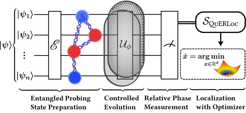
Figure 1. Workflow of QuERLoc

In this paper, we foresee an emerging opportunity in quantum-based ranging to break such limits for next-generation localization systems. We propose QuERLoc, a localization approach assisted by Quantum-Enhanced Ranging (QuER), which aims to concurrently tackle the co-existence of Gaussian noise accumulation from iterative ranging process, and the non-convexity objective arise from solving error minimization problem (Biswas et al., 2006). By introducing quantum metrology (Giovannetti et al., 2004, 2006, 2011) and quantum control theory (D’Alessandro, 2021; Shapiro and Brumer, 2006) and harnessing entangled probing states, QuER measures the Euclidean distances between the target and anchor nodes in a correlated manner rather than an isolated one. Schematic diagram is shown in Fig. 1. Quantum metrology infers the parameter related to distance ranging based on the physical dynamics of the probing system. In this context, we employ quantum bits, known as qubits, to approximate the probes in use. By manually controlling the dynamics of a qubit and utilizing the unique property of quantum entanglement, we expect that the readout from the metrology system would admit a linear combination of the square of distances through the solution of governing Schrödinger equation (Lec, 2006; Nielsen and Chuang, 2012). While classical ranging methods can algorithmically compute such combinations through repeated measurements, this approach tends to increase overhead and exacerbate measurement errors. In contrast, QuER exploits the inner tension among entangled qubits, enabling the measurement of sophisticated distance combinations with the same level of error as a single target-anchor distance measurement.

A salient feature of QuERLoc is that by preparing a special probing state corresponding to specific scheme of distance combination, the induced MLE problem would be convexified. Solving the induced optimization would be computationally efficient through computing a least-square (LS) regression (Van Huffel and Zha, 1993), while the derived solution maintains substantial reliability even when subjected to typical noise conditions. By a generic configuration of QuER scheme, $d$ rangings are adequate for QuERLoc to generate highly dependable position estimation in $d$-dimensional space. To validate our study, we conducted simulations with noisy distance ranging readouts. The results show that QuERLoc significantly outperforms baseline approaches using classical ranging, reduces the error metric RMSE by at least 73% and the average time consumption by at least 97.6%, and consistently saturates the theoretical lower bound of RMSE.

To the best of our knowledge, we are the first to study localization approaches based on quantum ranging. Our research takes a pioneering step towards the utilization of quantum-enhanced ranging with quantum entanglement for next-generation localization technologies. We believe this would provide insight to the mobile computing community, and open innovative research opportunities in the fields of both sensor network localization and quantum computing. Our contributions are summarized as follows:

• We introduce the problem of range-based quantum localization to the community for the first time and present an analytical formulation of a novel localization approach using quantum-enhanced ranging.

• We propose QuER, which utilizes the evolutionary dynamics of quantum probe under certain external field manipulation and the methodologies in quantum metrology.

• We formulate the localization problem of QuERLoc under specific probing scheme of QuER, resulting in a convex optimization problem that can be efficiently solved via weighted least-square regression, and requires only $d$ rangings for localization in $d$-dimensional space.

• We experimentally demonstrate that the proposed QuERLoc outperforms conventional range-based localization approaches significantly in accuracy and latency, and saturates the Cramér-Rao Lower Bound (CRLB) consistently.

The rest of the paper is organized as follows. We summarize related works in §2, and present a primer on quantum metrology and classical ranging in §3. We formulate probing particle dynamics in §4, followed by ranging model in §5 and localization algorithm in §6. §7 reports the evaluation results and §8 concludes the paper.

2. Related Works

Range-based Localization Range-based localization has been a subject of intense study, which involves two key problems: ranging and localization. Ranging is usually done by reversing the propagation distances from various signals, e.g., GPS, WiFi, mmWave, ultrasound, etc, with different ranging models, e.g., AoA, TDoA, RSSI, etc. Many efforts have been made towards localization with certain structure of distance information, including the trilateration-based algorithms, conic relaxation, and MDS-MAP.

Solving problems induced by trilateration often requires the use of linearization or pseudo-linearization (Lin et al., 2013), and the performance deteriorates significantly due to inaccurate distance measurements and error accumulation, thus further refinement is required (Biswas et al., 2006). In (Yang et al., 2009a; Xiao et al., 2018), noise-tolerant trilateration-based algorithms are proposed.

Localization by conic relaxation converts non-convex constraints in the problem formulation into convex ones. In (So and Ye, 2006), So and Ye studied the theory of semidefinite programming (SDP) in sensor network localization, while in (Yang et al., 2009b), Luo et al. applied SDP technique to TDoA localization. Tseng (Tseng, 2007) proposed second-order cone programming (SOCP) method as an efficient variant of SDP. Although relaxation method achieves high accuracy in estimating sensor locations, its complexity is in general not satisfactory (Han, 2000), and is thus only applicable to small-scale problems.

Multidimensional scaling (MDS) is a special technique aimed at finding low-dimensional representations for high-dimensional data. MDS-MAP (Shang et al., 2003) constructs a relative map through distance matrix, and localizes, nodes by transforming the map into a absolute map with sufficient and accurate distance measurements.

Quantum Metrology Quantum metrology (Giovannetti et al., 2004, 2006, 2011) emerged as an increasingly important research area, where quantum entanglement and coherence are harnessed to boost the precision of sensing beyond the limit of classical sensors in various fundamental scenarios, including thermometry (Mehboudi et al., 2019), reference frame alignment (Chiribella et al., 2004), and distance measurement (Giovannetti et al., 2001). Controlled evolution of quantum system is also widely studied, largely based on the control theory so as to create certain state evolution in realizing different sensing tasks (Shapiro and Brumer, 2006; Goyal et al., 2012). Besides theoretical works, a primitive quantum sensor network has been lately implemented (Liu et al., 2020), while recent experiment has demonstrated the feasibility of generating large Greenberger–Horne–Zeilinger (GHZ) state (Zhang et al., 2022). Experimental works demonstrate the feasibility to prepare widely-used probes in quantum metrology, including the ones utilized by QuERLoc.

Quantum-assisted Localization There is no significant amount of work presented in the interdisciplinary field of quantum information and localization. A few existing works enhance fingerprint-based localization by accelerating computation in fingerprint database searching using quantum algorithms. Grover in (Grover, 1997) improves the asymptotic time of searching in an unstructured dataset from $O(n)$ to $O(\sqrt{n})$. Buhrman et al. (Buhrman et al., 2001) introduces the concept of quantum fingerprints and proves its exponential improvement in storage complexity compared to classical one. Subsequent works include the quantum fingerprint localization (Shokry and Youssef, 2022), two-stage transmitter localization method with quantum sensor network (Zhan and Gupta, 2023), and machine learning-based WiFi sensing localization augmented with quantum transfer learning (Koike-Akino et al., 2022). To our awareness, there is no prior work on range-based localization with quantum ranging.

3. Preliminaries

3.1. Range-based Localization Model

A typical range-based localization model on a $d$-dimensional space where $d\in\{2,3\}$ consists of $n$ nodes with accurate positions $\texttt{Anc}=\{\bm{a}_{1},\dots,\bm{a}_{n}\}$ fixed on $\mathbb{R}^{d}$ under arbitrary topology, called the anchors. We consider an idealized picture of localization, where all facilities involved have full knowledge of the correspondence and localization of all available anchors. A sensor at position $\bm{x}\in\mathbb{R}^{d}$ communicates with a subset of Anc through certain medium and acquires information on the functionals of sensor-anchor distances, denoted as $\mathcal{S}(\{d_{i}:\leavevmode\nobreak\ i\in I\subset\{1,\dots,n\}\}|\bm{\vartheta})$ where $I$ is an index set indicating the indices of utilized anchors, $d_{i}:=\|\bm{x}-\bm{a}_{i}\|$ where $\|\cdot\|$ is the Euclidean norm on $\mathbb{R}^{d}$, and $\bm{\vartheta}$ parameterizes the ranging process. We herein refer to this process as ranging. Moreover, we assume the anchors and sensor positions are bounded, i.e., there exist scalars $0<\kappa_{a},\kappa_{s}<\infty$, such that for $1\leq i\leq n$, $\|\bm{a}_{i}\|_{\infty}\leq\kappa_{a}$ and $\|\bm{x}\|_{\infty}\leq\kappa_{s}$ where $\|\cdot\|_{\infty}$ stands for the vector infinite norm with $\|\bm{v}\|_{\infty}:=\max_{i}|v_{i}|$. Suppose a total of $m$ rangings are available, the objective of the sensor is to fully exploit available information $\{\mathcal{S}^{(k)}\}_{k=1}^{m}$ where the superscript $k$ specifies the signal acquired from the $k^{\text{th}}$ ranging, and estimate its position $\hat{\bm{x}}\in\mathbb{R}^{d}$.

3.2. Comparing Classic Ranging and QuER

Conventional range-based localization protocols have different distance measurement scenarios, each corresponds to a specific form of signal-distance mapping $\mathcal{S}(\cdot)$. The majority of such mapping involves one or two anchors, including the angle of arrival (AoA), $\mathcal{S}_{\text{AoA}}(d_{i}|\theta,\lambda)=2\pi\frac{\cos\theta}{\lambda}d_{i}$ where $\mathcal{S}_{\text{AoA}}$ is the phase difference of adjacent antennas; the time of arrival (ToA), $\mathcal{S}_{\text{ToA}}(d_{i}|v)=\frac{2d_{i}}{v}$ where $\mathcal{S}_{\text{ToA}}$ is the time difference between signal emission and recapture; the time differences of arrivals (TDoA), $\mathcal{S}_{\text{TDoA}}(d_{i},d_{j}|v)=\frac{1}{v}\left|d_{i}-d_{j}\right|$ where $\mathcal{S}_{\text{TDoA}}$ is the time differences of arrival at the paired and synchronized sensors; and the received signal strength indicator (RSSI), $\mathcal{S}_{\text{RSSI}}(d_{i}|P_{t},G_{t},G_{r},\lambda)=\frac{P_{t}G_{t}G_{r}\lambda^{2}}{16\pi^{2}d_{i}^{2}}$ where $\mathcal{S}_{\text{RSSI}}$ is the received signal power at the sensor (Mao et al., 2007).

A notable drawback of classic ranging is the requirement for target-anchor distances to be measured sequentially and individually, as in the cases of AoA, ToA, and RSSI, or in pairs for TDoA. Large numbers of ranging would be imperative if full utilization of anchors is required. This sequential measurement process not only introduces extra complexity and overhead of ranging into the localization task but also results in the system’s vulnerability to noise and environmental fluctuations, as the overall effect of normal noise integrated in distance $d_{i}$ to the eventual solution would be unpredictable. Moreover, substituting the primitive form of $\mathcal{S}(\cdot)$ into the localization problem arising from either MLE or error minimization (Biswas et al., 2006) always introduces computationally expensive optimization problems (Xiao et al., 2018).

In contrast, the Quantum-Enhanced Ranging (QuER) emerges as an innovative advancement, endowed with a unique capability in settling both issues. It enables the simultaneous ranging of a special combination of distances between a target sensor and an arbitrary number of anchors within a single physical measurement, which is nearly impossible to achieve in classical systems and allows a convexified localization problem. In the following section, we will present a primer on quantum metrology, which underpins QuER, while leaving the analysis of the exact form of the proposed quantum-enhanced ranging $\mathcal{S}_{\textsc{QuERLoc}}$ to §5.2.

3.3. Quantum Metrology

The proposed QuER is based on quantum metrology. We first briefly introduce the principles of quantum metrology and present its generic readout scenarios.

3.3.1. Quantum Metrology for Parameter Measurement

Quantum metrology targets measuring physical parameters with high precision with the aid of quantum mechanics principles (Giovannetti et al., 2006). It typically includes (i) Preparing a probe, described by a quantum state $\ket{\psi}$ in the environment with underlying Hilbert space $\mathcal{H}$, which under an orthornormal basis $\{\ket{n}\}$ of $\mathcal{H}$ can be expressed as $\ket{\psi}=\sum_{n}a_{n}\ket{n}$ and physically exhibits state $\ket{n}$ with probability $|a_{n}|^{2}$, subject to $\sum_{n}|a_{n}|^{2}=1$ (Nielsen and Chuang, 2012); (ii) Letting it interact with external system, which can be represented by a unitary transformation $\mathcal{U}_{\phi}$ encoded with targeted parameter set $\phi$; and (iii) Extracting information on $\phi$ by quantum measurement, specified by a set of measurement operators $\{\Pi_{i}\}_{i\in\mathbb{N}}$.

The probe state and measurement operators may assume to be either separable, or entangled (Giovannetti et al., 2006), corresponding to whether it is feasible to find the decomposition $\ket{\psi}=\ket{\psi_{1}}\otimes\cdots\otimes\ket{\psi_{n}}$, where $\ket{\psi_{i}}\in\mathcal{H}_{i}$ is the state in subspace $\mathcal{H}_{i}\subset\mathcal{H}$, and $\otimes$ represents the tensor product operation. QuERLoc employs this procedure as a subroutine to decode multiple sensor-anchor distances information from the entangled state with one-shot ranging.

3.3.2. Generic Readout Scenario of Quantum Metrology

A generic framework of an atomic probing system is encompassed by the following: Practically, the probe is prepared as a uniform superposition $\ket{\psi_{\text{init}}}=\frac{1}{\sqrt{2}}\left(\ket{a}+\ket{b}\right)$, where $\ket{a},\ket{b}$ are arbitrary orthonormal states in the space $\mathcal{H}$ (Giovannetti et al., 2006; Pezzé and Smerzi, 2014). Applying the parameterized unitary operation $\mathcal{U}_{\phi}$ on $\ket{\psi_{\text{init}}}$ yields the phase state (Giovannetti et al., 2011):

(1) $$\ket{\psi_{\phi}}=\frac{1}{\sqrt{2}}\left(\mathcal{U}_{\phi}\ket{a}+\mathcal{U}_{\phi}\ket{b}\right)\propto\frac{1}{\sqrt{2}}\left(\ket{a}+e^{-i\phi}\ket{b}\right).$$

Let $\Pi:=\ket{\psi_{\text{init}}}\bra{\psi_{\text{init}}}$ denote the projection operator on subspace spanned by the probe, we apply the positive operator-valued measurement (POVM) (Nielsen and Chuang, 2012) on $\ket{\psi_{\phi}}$, specified by a couple $\{\Pi,\bm{1}_{\mathcal{H}}-\Pi\}$ where $\bm{1}_{\mathcal{H}}$ is the identity map on $\mathcal{H}$. The readout process involves verifying whether $\ket{\psi_{\phi}}$ resides in the subspace of $\ket{\psi_{\text{init}}}$. The outcome would simply be either ‘yes’ (encoded as 0) or ‘no’ (encoded as 1), associated with probabilities

(2) $$\left\{\begin{aligned} &\text{Pr}(\text{outcome}=0)=\text{Tr}\left(\Pi\ket{\psi_{\phi}}\bra{\psi_{\phi}}\right)=\cos^{2}\frac{\phi}{2},\\ &\text{Pr}(\text{outcome}=1)=1-\text{Pr}(\text{outcome}=0)=\sin^{2}\frac{\phi}{2}.\end{aligned}\right.$$

Repeating the procedures allows us to analyze the value of $\phi$ with statistical tools such as maximum likelihood estimator and Bayesian inference (Pezzé and Smerzi, 2014).

In particular, when $\ket{a},\ket{b}$ are in $N$-tensor form, i.e., $\ket{a}=\ket{a_{1}}\otimes\cdots\otimes\ket{a_{N}}$ and $\ket{b}=\ket{b_{1}}\otimes\cdots\otimes\ket{b_{N}}$, while the operator $\mathcal{U}_{\phi}$ admits decomposition $\mathcal{U}_{\phi}=\mathcal{U}_{\phi_{1}}\otimes\cdots\otimes\mathcal{U}_{\phi_{N}}$, as the subscripts index the subsystem $\mathcal{H}_{i}$ the quantum states and operators live on. By nature of tensor product, relative phase can thus be alternatively expressed as the sum of relative phases in subsystems, specified by:

(3) $$\mathcal{U}_{\phi}\ket{\psi_{\text{init}}} =\frac{1}{\sqrt{2}}\left(\mathcal{U}_{\phi_{1}}\ket{a_{1}}\otimes\cdots\otimes\mathcal{U}_{\phi_{N}}\ket{a_{N}}\right.$$

$$+\left.\mathcal{U}_{\phi_{1}}\ket{b_{1}}\otimes\cdots\otimes\mathcal{U}_{\phi_{N}}\ket{b_{N}}\right)$$

$$\propto\frac{1}{\sqrt{2}}\left(\ket{a_{1}}\otimes\cdots\otimes\ket{a_{N}}+e^{-i\phi_{1}}\ket{b_{1}}\otimes\cdots\otimes e^{-i\phi_{N}}\ket{b_{N}}\right)$$

$$=\frac{1}{\sqrt{2}}\left(\ket{a}+e^{-i\sum_{j=1}^{N}\phi_{j}}\ket{b}\right).$$

Quantum metrology utilizes the above phase accumulation phenomenon to improve the asymptotic error by an $N^{-1/2}$ factor when detecting physical quantities, compared to classical metrology system (Giovannetti et al., 2011). QuER operates on an alternative advantage of this unique entanglement property. By deliberately correlate each relative phase $\phi_{j}$ with the particle’s travel distance, or equivalently, its time-of-flight (ToF), it enables multiple distances information to be encoded into the joint relative phase $\phi:=\sum_{j=1}^{N}\phi_{j}$. The following sections §4 and §5 will elaborate on the specific time-dependent evolution of a unique quantum state under certain external controls that QuER would use.

4. Controlled Dynamics of A Qubit

The controlled electrodynamics of quantum particles under the theory of quantum mechanics is crucial to the realization of QuER and our proposed QuERLoc. For an isolated physical system with Hamiltonian $H$, the dynamic of any time-dependent quantum state $\ket{\psi(t)}$ in the Hilbert space is governed by the following Schrödinger equation (Lec, 2006),

(4) $$i\hbar\frac{\partial}{\partial t}\ket{\psi(t)}=H\ket{\psi(t)},$$

where $\hbar$ is the reduced Planck constant, $i:=\sqrt{-1}$, and $\partial/\partial t$ is the partial derivative operator with respect to time. Specifically, we consider a two-level approximation (Lec, 2006) of an arbitrary particle, where only two energy levels are considered among multiple possible energy states. The two-level system includes a state of the lowest energy level, called the ground state with notion $\ket{g}$ and energy $E_{g}$, and a state with energy increased through energy absorption with external circumstance, called the excited state with notion $\ket{e}$ and energy $E_{e}$. The energy difference can be expressed as $\Delta E=E_{e}-E_{g}=\hbar\omega_{0}$, where $\omega_{0}$ is the particle frequency according to the theory of Louis de Broglie (Lec, 2006; Nielsen and Chuang, 2012).

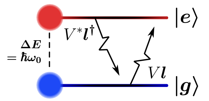
Figure 2. Dynamics of qubit with coupled energy levels

The external electromagnetic field can be viewed as a mechanism coupling the two energy levels, resulting in some implicit transitions between them. Precisely, we denote $\dagger$ to be the conjugate transpose of operators and states, $\bra{\psi}:=\ket{\psi}^{\dagger}$, $\bm{l}:=\ket{e}\bra{g}$ the atomic laddering operator (Lec, 2006) transiting the ground state to the excited one, and $\bm{l}^{\dagger}=\ket{g}\bra{e}$ the atomic descending operator acting the opposite, as shown in Fig. 2. Then the exact manner of such a coupling mechanism can be expressed as $V\bm{l}+\left(V\bm{l}\right)^{\dagger}$ (Nielsen and Chuang, 2012), where $V\in\mathbb{C}$ is a complex scalar function characterizing the coupling behaviour. For conciseness, we choose $E_{0}=\hbar\omega_{0}/2$ to be the energy zero level, thereby the Hamiltonian of the coupled system (Lec, 2006) can be formulated by:

(5) $$H=\frac{\hbar\omega_{0}}{2}\left(\bm{l}\bm{l}^{\dagger}-\bm{l}^{\dagger}\bm{l}\right)+V\bm{l}+V^{*}\bm{l}^{\dagger},$$

where $V^{*}$ represents the conjugate of complex number $V$.

The two-level approximation enables us to encode the states $\{\ket{e},\ket{g}\}$ into a single qubit by defining $\ket{0}:=\ket{e}$ and $\ket{1}:=\ket{g}$, and $\{\ket{0},\ket{1}\}$ would form an orthornormal basis of underlying Hilbert space. To investigate how the qubit would evolve when the external mechanism is manually controlled, we hereby consider the time-dependent coupling $V(t)=\epsilon(t)e^{i\theta(t)}$, where $\epsilon,\theta$ are coupling magnitude and field spinning rate respectively, both are real functionals on the time horizon $\mathcal{T}=[0,\infty)$. Analytical intractability of solving the Schrördinger equation with time-dependent Hamiltonian can be settled by a separation of operator: Consider the decomposition of $H$ (Mitarai et al., 2023) as $H=H_{0}+D(t)$, where $H_{0}$ is a time-independent full-rank operator (i.e., $\text{rank}H_{0}=\dim\mathcal{H}$), and $D(t)$ incorporates time-dependent terms. Suppose $H_{0}$ admits spectrum $\{E_{j}\}$ with eigenstates $\{\ket{j}\}$, then by assuming $\ket{\psi(t)}=\sum_{j}c_{j}(t)e^{-iE_{j}/\hbar t}\ket{j}$ with $c_{j}(t)$ being undetermined time-dependent coefficients, constraints on $c_{j}(t)$ can be derived in light of (4):

(6) $$i\hbar\frac{\partial}{\partial t}c_{j}(t)=\sum_{k}c_{k}(t)\exp\left\{-\frac{i}{\hbar}(E_{k}-E_{j})t\right\}\bra{j}D(t)\ket{k}.$$

Applying (6) to our proposed case, set $H_{0}=\frac{\hbar\omega_{0}}{2}\left(\bm{l}\bm{l}^{\dagger}-\bm{l}^{\dagger}\bm{l}\right)$, and $D(t)=V(t)\cdot\bm{l}+V^{*}(t)\cdot\bm{l}^{\dagger}$, the coefficients $c_{0}(t),c_{1}(t)$ should satisfy

(7) $$\left\{\begin{aligned} &\frac{\partial}{\partial t}c_{0}(t)=-\frac{i}{\hbar}\epsilon(t)e^{i(\theta(t)+\omega_{0}t)}c_{1}(t),\\ &\frac{\partial}{\partial t}c_{1}(t)=-\frac{i}{\hbar}\epsilon(t)e^{-i(\theta(t)+\omega_{0}t)}c_{0}(t).\end{aligned}\right.$$

Formulating the above coupled differential equations would yield the following equation:

(8) $$\frac{\partial^{2}}{\partial t^{2}}c_{j}(t) -\left\{\frac{1}{\epsilon(t)}\frac{\partial}{\partial t}\epsilon(t)+i\cdot(-1)^{j}\left(\frac{\partial}{\partial t}\theta(t)+\omega_{0}\right)\right\}\frac{\partial}{\partial t}c_{j}(t)$$

$$+\frac{\epsilon^{2}(t)}{\hbar^{2}}c_{j}(t)=0,\quad j=0,1.$$

A tentative solution would be $c_{j}(t)\propto e^{i\eta_{j}(t)}$ where $\eta_{j}$ is a real funtional on $\mathcal{T}$. Substituting it into (8) yields following equation:

(9) $$\left(\frac{\partial}{\partial t}\eta_{j}(t)\right)^{2} -(-1)^{j}\left(\frac{\partial}{\partial t}\theta(t)+\omega_{0}\right)\frac{\partial}{\partial t}\eta_{j}(t)-\frac{\epsilon^{2}(t)}{\hbar^{2}}$$

$$=i\left(\frac{\partial^{2}}{\partial t^{2}}\eta_{j}(t)-\frac{\frac{\partial}{\partial t}\epsilon(t)}{\epsilon(t)}\frac{\partial}{\partial t}\eta_{j}(t)\right),\quad\forall j=0,1.$$

Since $\eta_{j},\epsilon,\phi$ are all real functionals, the coincidence of two sides in above equation demonstrates the following constraints on the form of quantum state:

(10) $$\begin{array}[]{cl}\ket{\psi(t)}=&\sum_{j=0,1}\sum_{\eta_{j}}Q_{\eta_{j}}e^{i(\eta_{j}(t)-(-1)^{j}\omega_{0}t/2)}\ket{j},\\ \text{s.t.}&\left(\frac{\partial}{\partial t}\eta_{j}(t)\right)^{2}-(-1)^{j}\left(\frac{\partial}{\partial t}\phi(t)+\omega_{0}\right)\frac{\partial}{\partial t}\eta_{j}(t)\\ &-\frac{\epsilon^{2}(t)}{\hbar^{2}}=0,\\ &\left(\frac{\partial}{\partial t}\eta_{j}(t)\right)^{-1}\frac{\partial^{2}}{\partial t^{2}}\eta_{j}(t)=\epsilon^{-1}(t)\frac{\partial}{\partial t}\epsilon(t),\end{array}$$

where $Q_{\eta_{j}}\in\mathbb{C}$ are complex coefficients, and the inner summations are taken on all possible functionals $\eta_{j}$. The exact behaviour of state entries can be solved with full knowledge of its initial state $\ket{\psi(0)}$ and coupling factors $(\epsilon(t),\phi(t))$.

5. Quantum-Enhanced Ranging

In this section, we discuss in detail how our QuERLoc takes advantage of a special case of the above constrained probe qubit evolution. Within the region of localization, we deploy a meticulously controlled field with $\epsilon(t)=\nu(2\gamma t+\omega_{0})$ and $\theta(t)=\gamma t^{2}$, where $\nu,\gamma>0$ are positive parameters. We further assume that $\nu\gg\hbar$.

5.1. Behaviour of Qubit with Uniform Superposition

We begin with illustrating the evolutionary behaviour of a qubit $\ket{\psi(0)}$ with uniform quantum superposition state, i.e., it admits equal probability on both of its energy states. It can be prepared by implementing the Hadamard transformation (Nielsen and Chuang, 2012) $\mathscr{H}$ on $\ket{0}$:

(11) $$\ket{\psi(0)}=\mathscr{H}\ket{0}=\frac{1}{\sqrt{2}}\left(\ket{0}+\ket{1}\right).$$

From the expression of $\epsilon,\theta$, we could arrive at an expression of the time variation of single-qubit state $\ket{\psi(t)}$:

(12) $$\ket{\psi(t)}=c_{0}(t)e^{-\omega_{0}t/2}\ket{0}+c_{1}(t)e^{\omega_{0}t/2}\ket{1},$$

subject to the initial state consistency and probability completeness

(13) $$c_{0}(0) =c_{1}(0)=\frac{1}{\sqrt{2}},\quad\left|c_{0}(t)\right|^{2}+\left|c_{1}(t)\right|^{2}=1,\quad j=0,1,$$

$$c_{j}(t) =A_{j}\exp\left\{i\cdot\frac{(-1)^{j}+\sqrt{1+4\nu^{2}/\hbar^{2}}}{2}(\gamma t^{2}+\omega_{0}t)\right\}$$

$$+B_{j}\exp\left\{i\cdot\frac{(-1)^{j}-\sqrt{1+4\nu^{2}/\hbar^{2}}}{2}(\gamma t^{2}+\omega_{0}t)\right\}.$$

Denote $\Re(C)$ and $\Im(C)$ as the real and imaginary part of a complex number $C\in\mathbb{C}$. Solving the undetermined coefficients $A_{j},B_{j}\in\mathbb{C}$ for $j=0,1$ in (13) subject to (7), we discover that

(14) $$\left\{\begin{aligned} &\Re(A_{0})=\frac{1}{\sqrt{2}}\frac{1-\tau}{1+\tau^{2}},\quad\Re(B_{0})=\frac{1}{\sqrt{2}}\frac{\tau^{2}+\tau}{1+\tau^{2}},\\ &\Re(A_{1})=\frac{1}{\sqrt{2}}\frac{\tau^{2}-\tau}{1+\tau^{2}},\quad\Re(B_{1})=\frac{1}{\sqrt{2}}\frac{\tau+1}{1+\tau^{2}},\\ &\Im(A_{0})=\Im(A_{1})=\Im(B_{0})=\Im(B_{1})=0,\\ &\tau=\frac{2\nu/\hbar}{1+\sqrt{1+4\nu^{2}/\hbar^{2}}}.\end{aligned}\right.$$

By denoting $\Delta(t):=-\sqrt{1+4\nu^{2}/\hbar^{2}}\left(\gamma t^{2}+\omega_{0}t\right)$, the previous assumption $\nu\gg\hbar$ indicates that $2\nu/\hbar\gg 1$, and consequently $\tau\to 1$. Note that whenever $|\Re(e^{i\Delta(t)})|=\left|\cos(\Delta(t))\right|\gg\frac{1-\tau}{\tau^{2}+\tau}$, we have two approximate relations $A_{0}+B_{0}e^{i\Delta(t)}\approx\frac{1}{\sqrt{2}}e^{i\Delta(t)}$ and $A_{1}+B_{1}e^{i\Delta(t)}\approx\frac{1}{\sqrt{2}}e^{i\Delta(t)}$. When $\Delta(t)=\pm\frac{\pi}{2}+\varepsilon$ for some scalar $|\varepsilon|\ll 1$ within a period $2\pi$ of the $\cos(\cdot)$ function, $|\cos(\Delta(t))|=|\sin(\pm\frac{\pi}{2}-\Delta(t))|=|\sin(\varepsilon)|\approx|\varepsilon|$. Thus, when $\varepsilon$ satisfies $\frac{1-\tau}{\tau^{2}+\tau}\ll|\varepsilon|\ll 1$, e.g., $\varepsilon=\sqrt{\frac{1-\tau}{\tau^{2}+\tau}}$, the following approximation of probe state dynamic can be applied except for intervals $\left[\pm\frac{\pi}{2}-|\varepsilon|,\pm\frac{\pi}{2}+|\varepsilon|\right]$ within a single period:

(15) $$\ket{\psi(t)} =\frac{1}{\sqrt{2}}{e^{-\frac{i\omega_{0}}{2}t}e^{i\cdot\frac{1+\sqrt{1+4\nu^{2}/\hbar^{2}}}{2}\left(\gamma t^{2}+\omega_{0}t\right)}}\left(\frac{1-\tau}{1+\tau^{2}}+\frac{\tau^{2}+\tau}{1+\tau^{2}}e^{i\Delta(t)}\right)\ket{0}$$

$$+\frac{1}{\sqrt{2}}{e^{\frac{i\omega_{0}}{2}t}e^{i\cdot\frac{-1+\sqrt{1+4\nu^{2}/\hbar^{2}}}{2}(\gamma t^{2}+\omega_{0}t)}}\left(\frac{\tau^{2}-\tau}{1+\tau^{2}}+\frac{\tau+1}{1+\tau^{2}}e^{i\Delta(t)}\right)\ket{1}$$

$$\xrightarrow{\tau\to 1,\leavevmode\nobreak\ |\cos(\Delta(t))|\gg\frac{1-\tau}{\tau^{2}+\tau}}\leavevmode\nobreak\ \underbrace{e^{\frac{i}{2}\gamma t^{2}}e^{\frac{i}{2}\Delta(t)}}_{\text{global phase}}\left(\frac{\ket{0}+e^{-i\gamma t^{2}}\ket{1}}{\sqrt{2}}\right)$$

$$\propto\frac{\ket{0}+e^{-i\gamma t^{2}}\ket{1}}{\sqrt{2}}.$$

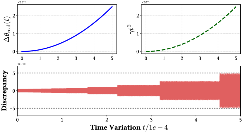
Figure 3. Comparison of real relative phase $\Delta\theta_{\text{real}}(t)$ and $\gamma t^{2}$. Minor outliers ($50$ out of $5\times 10^{6}$ data points) are filtered out. Here we set $\gamma=10^{3}\leavevmode\nobreak\ \text{rad}/\text{sec}^{2}$, $\omega_{0}=10^{-2}\leavevmode\nobreak\ \text{rad}/\text{sec}$, and $\nu/\hbar=10^{10}$. $\frac{1-\tau}{\tau^{2}+\tau}=2.5\times 10^{-11}$. Absolute discrepancy is bounded by $5\times 10^{-10}$ while relative phase is on the order of $10^{-4}$. Parameters can be adjusted subject to prior estimation on the order of probe ToF.

Such approximation is feasible with a high probability of $1-\frac{2|\varepsilon|}{\pi}$, and its validity over a certain time period is demonstrated numerically in Fig. 3. While the global phase factor could not be statistically observed (Nielsen and Chuang, 2012), the two energy states yield a time-dependent relative phase shift with angular speed proportional to the square of time $t$, which enables the statistical detection of qubit ToF in quadratic form (Giovannetti et al., 2011), as outlined in §3.3.2.

5.2. Ranging Model of QuERLoc

Previous analysis in §5.1 could be naturally extended to the picture of multi-qubit evolution. This is of great essence to the realization of QuERLoc. Prior to that, we first outline the settings of our proposed quantum-enhanced ranging. Analogous to classical range-based localization, a QuERLoc scheme conducts a total of $m$ rangings (QuERs), whereas for the $k^{\text{th}}$ ranging where $1\leq k\leq m$, the anchors involved would be flexibly identified by an index set $I_{k}\subset\{1,\dots,n\}$, by recalling that each index $i\in\{1,\dots,n\}$ stands for the $i^{\text{th}}$ anchor available. Each involved anchor $\bm{a}_{i}$ subject to $i\in I_{k}$, is assigned a binary-valued parameter $w_{i,k}\in\{-1,1\}$. $\{w_{i,k}\}_{i\in I_{k}}$ specifies the probe scheme of the $k^{\text{th}}$ QuER. Accordingly, denote $|\cdot|$ as the set cardinality and $\mathbbm{1}{(\cdot)}$ as the indicator function, each ranging would require the following maximally entangled $|I_{k}|$-qubit probe:

(16) $$\ket{\psi(0)}_{k} =\frac{1}{\sqrt{2}}\sum_{j=0,1}\bigotimes_{i\in I_{k}}\ket{\pi_{i,k}^{(j)}},$$

$$\pi_{i,k}^{(j)} =\mathbbm{1}{\{w_{i,k}=-1\}}+j\leavevmode\nobreak\ \text{mod}\leavevmode\nobreak\ 2,$$

which can be prepared by an entangling operator $\mathscr{E}_{k}\left(\{w_{i,k}\}_{i\in I_{k}}\right)$ on the input ground state, composed by a sequence of Hadamard gates, controlled-not (CNOT) gates and NOT (Pauli-X) gates (Nielsen and Chuang, 2012). An illustrative example on preparing a four-qubit probe $\frac{1}{\sqrt{2}}\left(\ket{0101}+\ket{1010}\right)$ that corresponds to QuER scheme $\{1,-1,1,-1\}$ is shown in Fig. 4.

$$\begin{array}[]{c}\Qcircuit@C=1em@R=1em{&\lstick{\ket{0}}&\gate{\mathscr{H}}&\ctrl{1}&\qw&\qw&\qw&\qw&\qw\\ &\lstick{\ket{0}}&\qw&\targ&\ctrl{1}&\qw&\qw&\gate{\sigma_{x}}&\qw\\ &\lstick{\ket{0}}&\qw&\qw&\targ&\ctrl{1}&\qw&\qw&\qw\\ &\lstick{\ket{0}}&\qw&\qw&\qw&\targ&\qw&\gate{\sigma_{x}}&\qw\gategroup{1}{3}{4}{6}{1em}{--}}\end{array}$$

Figure 4. Quantum circuit of ${\mathscr{E}(\{1,-1,1,-1\})}$ applied to $\ket{0}^{\otimes 4}$. The section outlined by dash line prepares a $4$-qubit GHZ state (Nielsen and Chuang, 2012), while the following $\sigma_{x}$ gates conduct bit-flipping.

To convexify the localization problem, QuERLoc further restricts that an even number of anchors are utilized for each ranging process of QuER (i.e., $|I_{k}|\in 2\mathbb{Z}$), and moreover

(17) $$\forall k,\quad\sum_{i\in I_{k}}\mathbbm{1}{\{w_{i,k}=1\}}=\sum_{i\in I_{k}}\mathbbm{1}{\{w_{i,k}=-1\}}.$$

The sensor triggers each ranging procedure by simultaneously emitting the entangled probe qubits, which subsequently evolve continuously in the controlled external field until getting received by the sensor after being reflected by the specific anchor. Denote $\bm{t}_{k}=\{t_{i}\}_{i\in I_{k}}$ the time instants at which each qubit is retrieved by the sensor, the probe would end up with the following form:

(18) $$\ket{\psi(\bm{t}_{k})}_{k} =\frac{1}{\sqrt{2}}e^{\frac{i}{2}\sum_{i\in I_{k}}\Delta(t_{i})}e^{i\xi_{k}}\left(\bigotimes_{i\in I_{k}}\ket{\pi_{i,k}^{(0)}}+e^{-i\chi_{k}}\bigotimes_{i\in I_{k}}\ket{\pi_{i,k}^{(1)}}\right)$$

$$\propto\frac{1}{\sqrt{2}}\left(\bigotimes_{i\in I_{k}}\ket{\pi_{i,k}^{(0)}}+e^{-i\chi_{k}}\bigotimes_{i\in I_{k}}\ket{\pi_{i,k}^{(1)}}\right),$$

where

(19) $$\chi_{k}=\gamma\sum_{i\in I_{k}}w_{i,k}t_{i}^{2},\quad\xi_{k}=\frac{1}{2}\chi_{k}.$$

Special quantum properties such as the Zeno effect (Itano et al., 1990) enable us to inhibit the successive spontaneous evolution once the qubit is returned. Thus, no time synchronization is required among different probing qubits, which is of great concern in traditional ToA and TDoA ranging models (Mao et al., 2007). With the relative phase $\chi$ acquired, by assuming photons are employed as the probes (Giovannetti et al., 2006), whose propagation speed is the speed of light $c$, we could use the instantaneous relation between distance and ToF $t_{i}=2d_{i}/c$ to derive the signal-distance mapping $\mathcal{S}_{\textsc{QuERLoc}}^{(k)}$ for all $k\in\{1,\dots,m\}$,

(20) $$\mathcal{S}_{\textsc{QuERLoc}}^{(k)}\left(\{d_{i}\}_{i\in I_{k}}|\{w_{i,k}\}_{i\in I_{k}},\gamma,c\right):=\chi_{k}=\frac{4\gamma}{c^{2}}\sum_{i\in I_{k}}w_{i,k}d_{i}^{2}.$$

Above non-linear ToF effect is an instance of quantum control that realizes nonlinear quantum dynamics with external field manipulation (Liu et al., 2003; Daems et al., 2013), which is of increasing interest in the field of quantum information processing. In the next section, we will reformulate the localization task as a simple optimization problem based on above structure of phase information.

6. Localization via Quantum Ranging

6.1. Reformulating the Phase-Distance Relations

Upon obtaining the accumulated phase $\chi_{k}$, we can further expand the terms in previous equality (20) as follows:

(21) $$\frac{4\gamma}{c^{2}}\sum_{i\in I_{k}}w_{i,k}d_{i}^{2} =\frac{4\gamma}{c^{2}}\sum_{i\in I_{k}}w_{i,k}\left(\bm{x}-\bm{a}_{i}\right)^{T}\left(\bm{x}-\bm{a}_{i}\right)$$

$$=\frac{4\gamma}{c^{2}}\underbrace{\sum_{i\in I_{k}}w_{i,k}}_{=\leavevmode\nobreak\ 0}\bm{x}^{T}\bm{x}-\bigg{(}\frac{8\gamma}{c^{2}}\sum_{i\in I_{k}}w_{i,k}\bm{a}_{i}\bigg{)}^{T}\bm{x}$$

$$+\frac{4\gamma}{c^{2}}\sum_{i\in I_{k}}w_{i,k}\bm{a}_{i}^{T}\bm{a}_{i}=\chi_{k},\quad\forall 1\leq k\leq m.$$

The coefficient of $\bm{x}^{T}\bm{x}$ is eliminated due to the requirement in (17). For mathematical brevity, we apply the following variable substitution after simplifying the equation in (21):

(22) $$\bm{L}=\begin{pmatrix}\bm{u}_{1},\dots,\bm{u}_{m}\end{pmatrix}^{T}\in\mathbb{R}^{m\times d},\quad\bm{h}=\begin{pmatrix}h_{1},\dots,h_{m}\end{pmatrix}^{T}\in\mathbb{R}^{m},$$

$$\bm{u}_{k}=2\sum_{i\in I_{k}}w_{i,k}\bm{a}_{i},\quad h_{k}=\sum_{i\in I_{k}}w_{i,k}\bm{a}_{i}^{T}\bm{a}_{i}-\left(4\gamma\right)^{-1}c^{2}\chi_{k}.$$

Finally, by aggregating results from all $m$ distance ranging, the simplification moves us from dealing with a complicated quadratic problem to working with the following elegant and straightforward system of linear equations, which QuERLoc solves to realize sensor positioning:

(23) $$\mathop{\text{Find}}\quad\bm{x}\in\mathbb{R}^{d},\quad\text{s.t.}\quad\bm{L}\bm{x}=\bm{h}.$$

6.2. Weighted Least-Square Solution

The systematic bias introduced by the relative phase readout can be modeled as Gaussian noise. It is routine to assume the noise in parallel experiments are independent, yield zero mean, and have standard deviation proportional to the magnitude of observable physical quantities (Biswas et al., 2006). Without loss of generality, we consider all noise are integrated in the scalarized value of signal $\left(4\gamma\right)^{-1}c^{2}\chi_{k}$, which we denote as $\lambda_{k}$. The noisy measurement readout can be analytically modeled as

(24) $$\widetilde{\lambda}_{k}=\lambda_{k}\left(1+\delta_{k}\right),\quad\bm{\delta}\sim\mathcal{N}\left(\bm{0},\rho^{2}\bm{I}\right),$$

where $\rho\in[0,1)$ is a scaling factor that characterizes the extent of measurement error, and $\bm{\delta}$ is a vector of Gaussian noise.

We use the $\mathbb{R}^{m}$ vectors $\bm{\lambda},\widetilde{\bm{\lambda}}$ respectively to aggregate the exact and noisy measurement readouts. Based on previous assumptions, on observing $\widetilde{\bm{\lambda}}$, the problem (23) can be addressed by solving the following log-likelihood maximization:

(25) $$\hat{\bm{x}} =\mathop{\arg\max}_{\bm{x}\in\mathbb{R}^{d}}\quad\log\mathcal{L}\left[\widetilde{\bm{\lambda}};\{w_{i,k}\}_{i\in I_{k}}:\leavevmode\nobreak\ 1\leq k\leq m;\leavevmode\nobreak\ \texttt{Anc}\right]$$

$$=\mathop{\arg\max}_{\bm{x}\in\mathbb{R}^{d}}\quad\log\mathop{\text{Pr}}\limits_{\bm{\delta}\sim\mathcal{N}(0,\rho^{2}\bm{I})}\left[\widetilde{\bm{\lambda}}\leavevmode\nobreak\ \bigg{|}\leavevmode\nobreak\ \widetilde{\lambda}_{k}=\lambda_{k}\left(1+\delta_{k}\right)\right]$$

$$=\mathop{\arg\max}_{\bm{x}\in\mathbb{R}^{d}}\quad\sum_{k=1}^{m}\log\bigg{[}\frac{1}{\sqrt{2\pi}\rho\lambda_{k}}\cdot e^{\frac{(u_{k}^{T}\bm{x}-h_{k}-\lambda_{k}+\widetilde{\lambda}_{k})^{2}}{2\rho^{2}\lambda_{k}^{2}}}\bigg{]}$$

$$\approx\mathop{\arg\min}_{\bm{x}\in\mathbb{R}^{d}}\quad\left\|\sqrt{\widetilde{W}}\left(\bm{L}\bm{x}-\widetilde{\bm{h}}\right)\right\|^{2}.$$

Alternatively, we use term $\widetilde{h}_{k}=\sum_{i\in I_{k}}w_{i,k}\bm{a}_{i}^{T}\bm{a}_{i}-\widetilde{\lambda}_{k}$ as the $k^{\text{th}}$ entry of vector $\widetilde{\bm{h}}$ with noise, and $\widetilde{W}=\text{diag}\left(\widetilde{\lambda}_{1}^{-2},\dots,\widetilde{\lambda}_{m}^{-2}\right)$ as the diagonal weighting matrix. Approximation in the last equality arises from our insufficient knowledge of the true measurement outcomes $\{\lambda_{k}\}_{k=1}^{m}$, and we thus replace them by the noisy observations.

Above optimization objective is a typical weighted least square (WLS) problem, which is convex and would yield a closed-form solution (Van Huffel and Zha, 1993):

(26) $$\hat{\bm{x}}_{\text{opt}}=\left(\bm{L}^{T}\widetilde{W}\bm{L}\right)^{-1}\bm{L}^{T}\widetilde{W}\widetilde{\bm{h}}.$$

It is worth noting that solving the QuERLoc problem requires relatively low computational complexity, as will be discussed in §7.2.4. Unlike traditional localization methods, our QuERLoc directly admits a convex optimization problem in its simplified expression and no further transformation is required.

7. Numerical Analysis

We present numerical analysis results in this section to demonstrate the performance of QuERLoc under different testbed settings.

7.1. Simulation Setups

7.1.1. Default Settings of Parameters

In subsequent experiments, we set up default values for a fraction of the parameters included, as listed in Tab. 1.

Table 1. Default settings of experiment parameters

Parameters	Value
Dimension ${d}$	$3$
${\kappa_{s}}$	$100$ (m)
${\kappa_{a}/\kappa_{s}}$	$0.5$
Number of Anchors ${n}$	$10$
Anc	$\left\{\begin{aligned} &(0,0,0),(\kappa_{a},0,0),(0,\kappa_{a},0)\\ &(0,0,\kappa_{a})(\kappa_{a},\kappa_{a},\kappa_{a}),(\kappa_{a},0,\kappa_{a})\\ &(\kappa_{a},\kappa_{a},0),(0,\kappa_{a},\kappa_{a}),\left(\frac{\kappa_{a}}{2},\frac{\kappa_{a}}{2},0\right)\\ &\left(\frac{\kappa_{a}}{2},\frac{\kappa_{a}}{2},\kappa_{a}\right)\end{aligned}\right\}$
Number of Ranging ${m}$	$3,4,5$
$\forall k,\quad{|I_{k}|}$	$2$
Noise factor ${\rho}$	$0\%-5\%$, step length $0.5\%$

In addressing an instance of localization problem , we can, without loss of generality, scale down all distance values by a coefficient, even if these values are of a very large magnitude. Thus, the choice of $\kappa_{s}$ would not affect the result of our numerical evaluation, and we simply set $\kappa_{s}=100$ (m) here. Note that we control the ratio $\kappa_{a}/\kappa_{s}$ to be smaller than $1$, so as to generate both near-field and far-field instances, while the latter case is notably more sensitive to ranging noise. Anchors are deployed at the very beginning of the experiment with the specified topology to avoid degeneration of the baseline performance, and remain stationary throughout the simulations. To ensure the feasibility of experimental realization in subsequent works, we employ a $2$-qubit entangled probe in the simulation, and thus $|I_{k}|=2$. Entries of signing scheme $\{w_{i,k}\}_{i\in I_{k}}$ will be specified in the later context, subject to various choices of number of rangings $m$.

7.1.2. Baseline Algorithms

We compare QuERLoc with three range-based localization approaches: (i) Multilateration + GD: multilateration is an enhanced version of trilateration to make the solution more robust to noise (Zhou and Shi, 2008; Xiao et al., 2014) by involving more shots of ranging. We further apply a gradient-descent (GD) refinement (Biswas et al., 2006) to the solution of the linear system introduced by multilateration in the presence of noise to provide a convincing baseline. (ii) SDP-based Localization: introduced to the field of sensor network localization in (So and Ye, 2006). It is a powerful approach to achieve robust positioning in network with complex topology, we reduce it to the case of single sensor localization. (iii) TDoA: set up the same reference anchor among all time-difference rangings, and locate the sensors by finding the intersection point of a set of elliptic curves with a shared focus. In the following experiment, we use Chan’s algorithm (Lin et al., 2013) to settle the non-convexity of distance terms by formulating a pseudo-linear system and solving it with SOCP (Han, 2000).

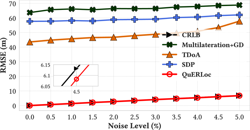
(a) RMSE, $m=3$

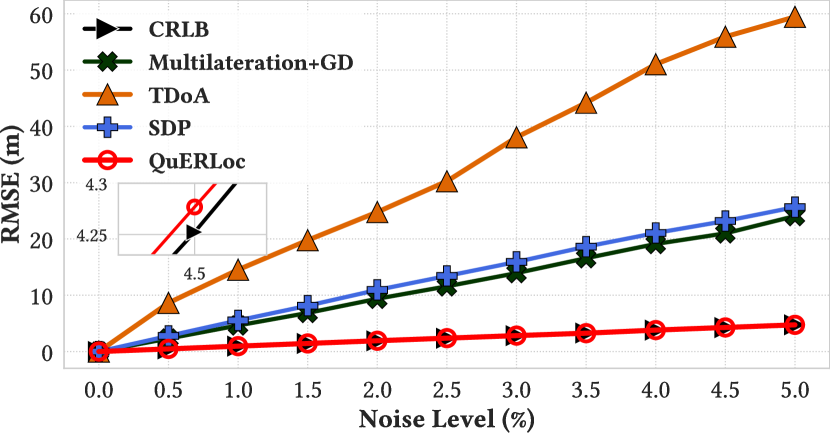
(b) RMSE, $m=4$

(c) RMSE, $m=5$

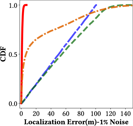
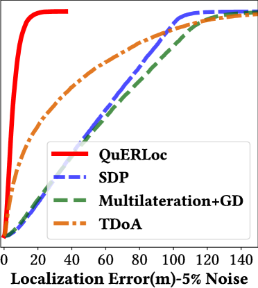
(d) CDF, $m=3$

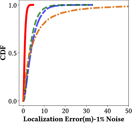
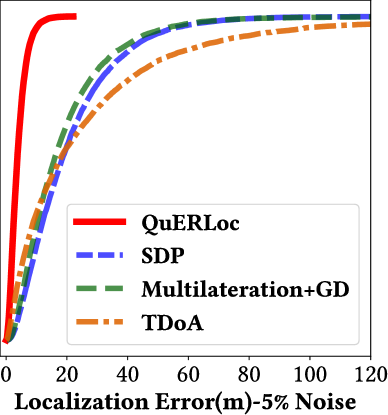
(e) CDF, $m=4$

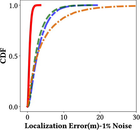
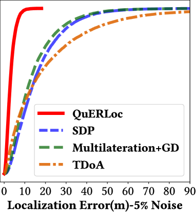
(f) CDF, $m=5$

Figure 5. Performance of QuERLoc and baselines over different noise levels. The CDF of localization error to all localization approaches when $m=3,4$ and $5$ are plotted under noise levels $1\%$ and $5\%$.

7.1.3. Performance Metrics

To evaluate the performance of a localization algorithm, we repeat the ranging and localization procedure under the same simulation settings, for a total of $r\in\mathbb{N}$ times. Denote $\hat{\bm{x}}^{(t)}$ and $\bm{x}^{(t)}:=\bm{x}_{\text{real}}^{(t)}$ to be the estimation and ground truth of the sensor location in the $t^{\text{th}}$ iteration. To measure the precision of all presented localization techniques, we examine both localization error $\left\|\hat{\bm{x}}^{(t)}-\bm{x}^{(t)}\right\|$ of a single experiment and Root-Mean-Square-Error (RMSE) (Yu et al., 2009) of $r$ iterative experiments at the same noise level. Specifically, the RMSE is defined by

$$\text{RMSE}:=\sqrt{\frac{1}{r}\sum_{t=1}^{r}\left\|\hat{\bm{x}}^{(t)}-\bm{x}^{(t)}\right\|^{2}}.$$

7.1.4. Cramér-Rao Lower Bound

Additionally, we examine the Cramér-Rao Lower Bound (CRLB) as a benchmark to gauge the optimal accuracy attainable by the estimator $\hat{\bm{x}}$ employed by QuERLoc. Recall that we derive the optimization objective in (25) through the following log-probability density function:

$$\log\mathcal{L}\left(\widetilde{\bm{\lambda}}^{(t)}\right) =-\sum_{k=1}^{m}\log\left(\sqrt{2\pi}\rho\widetilde{\lambda}_{k}^{(t)}\right)$$

$$-\frac{1}{2\rho^{2}}\left\|\sqrt{\widetilde{W}^{(t)}}\left(\bm{L}^{(t)}\bm{x}-\widetilde{\bm{h}}^{(t)}\right)\right\|^{2}.$$

The Fisher information matrix (Rissanen, 1996) of the log-likelihood function can be formulated as

(27) $$\mathcal{F}\left(\widetilde{\bm{\lambda}}^{(t)}\right) =-\mathbb{E}\left[\frac{\partial^{2}\log\mathcal{L}(\widetilde{\bm{\lambda}}^{(t)})}{\partial\bm{x}\partial\bm{x}^{T}}\right]=\left\{-\mathbb{E}\left[\frac{\partial^{2}\log\mathcal{L}(\widetilde{\bm{\lambda}}^{(t)})}{\partial x_{i}\partial x_{j}}\right]\right\}_{ij}$$

$$=\left\{\left(\bm{L}^{(t)}\frac{\partial^{2}\bm{x}}{\partial x_{i}\partial x_{j}}\right)^{T}\frac{1}{\rho^{2}}\mathbb{E}\left[\widetilde{W}^{(t)}\left(\bm{L}^{(t)}\bm{x}-\widetilde{\bm{h}}^{(t)}\right)\right]\right.$$

$$\left.+\frac{1}{\rho^{2}}\left(\bm{L}^{(t)}\frac{\partial\bm{x}}{\partial x_{i}}\right)^{T}\mathbb{E}\left[\widetilde{W}^{(t)}\right]\left(\bm{L}^{(t)}\frac{\partial\bm{x}}{\partial x_{j}}\right)\right\}_{ij}$$

$$\approx\frac{1+3\rho^{2}}{\rho^{2}}\left(\bm{L}^{(t)}\right)^{T}\widetilde{W}^{(t)}\bm{L}^{(t)}.$$

The first term in the summation vanishes due to $\frac{\partial^{2}\bm{x}}{\partial x_{i}\partial x_{j}}=\left[\frac{\partial\delta_{kj}}{\partial x_{i}}\right]_{k}=\bm{0}$. The final expression in (27) originates from $\partial\bm{x}^{T}/\partial\bm{x}=\bm{I}$, and $\mathbb{E}[\widetilde{\lambda}_{k}^{-2}]=\lambda^{-2}_{k}\cdot\mathbb{E}[1-2\delta_{k}+3\delta_{k}^{2}+O(\delta_{k}^{3})]\approx(1+3\rho^{2})\lambda_{k}^{-2}$ by Taylor expansion along with $\mathbb{E}[\delta_{k}]=0$ and $\mathbb{E}[\delta_{k}^{2}]=\text{Var}[\delta_{k}]+\mathbb{E}^{2}[\delta_{k}]=\rho^{2}$. CRLB provides a lowerbound $\mathbb{E}[(\hat{\bm{x}}^{(t)}-\bm{x}^{(t)})(\hat{\bm{x}}^{(t)}-\bm{x}^{(t)})^{T}]\succeq\mathcal{F}^{-1}(\widetilde{\bm{\lambda}}^{(t)})$. This allows us to derive a lowerbound for RMSE when $r$ is sufficiently large,

(28) RMSE $$\overset{r\gg 1}{=}\sqrt{\frac{1}{r}\sum_{t=1}^{r}\mathbb{E}\left[\left(\hat{\bm{x}}^{(t)}-\bm{x}^{(t)}\right)^{T}\left(\hat{\bm{x}}^{(t)}-\bm{x}^{(t)}\right)\right]}$$

$$=\sqrt{\frac{1}{r}\sum_{t=1}^{r}\text{Tr}\left(\mathbb{E}\left[\left(\hat{\bm{x}}^{(t)}-\bm{x}^{(t)}\right)\left(\hat{\bm{x}}^{(t)}-\bm{x}^{(t)}\right)^{T}\right]\right)}$$

$$\overset{\text{CRLB}}{\geq}\sqrt{\frac{1}{r}\sum_{t=1}^{r}\text{Tr}\left(\mathcal{F}^{-1}(\widetilde{\bm{\lambda}}^{(t)})\right)}.$$

7.2. Evaluation Results

We evaluate all the positioning instances on a classical computer. Within the same setup, we repeatedly generate $r=10^{4}$ locations and perturb the distances data in an analogous way to (24).

All approaches including QuERLoc and baselines (i)-(iii) will share identical testbed settings and estimate the same randomly generated sensor locations $\{\bm{x}^{(t)}\}_{t=1}^{r}$. The choices of used anchors are determined by the particular protocols of each localization method according to their selective strategies. Notice that we mainly focus on QuERLoc’s capability to acquire special distance combinations rather than the enhancement quantum metrology would bring to the readout precisions (Giovannetti et al., 2011). Thus, we set the factor $\rho$ to be identical among all approaches adopted at the same noise level.

We implemented all algorithms in Python, where the least-square regressions were solved using the built-in Python package numpy, and SOCPs/SDPs were solved using MOSEK (Dahl, 2012). All simulations were run on a Windows PC with 16GB memory and AMD Ryzen 9 7945HX CPU.

7.2.1. Performance with Few Numbers of Rangings.

For each choice of the number of rangings $m\in\{3,4,5\}$, we set the probe scheme to be $I_{k}=\{2k-1,2k\}\subset\{1,\dots,n\}$ and $w_{i,k}=-(-1)^{i}$ for $1\leq k\leq m$ and $i\in I_{k}$. QuERLoc exploits $m$ distinct pairs of anchors for one-shot localization. Baselines approaches, including TDoA (where one anchor serves as the reference node across all TDoA measurements), utilize $m$ anchors since each ranging only introduces information from a single new anchor. Fig. 5a, 5b and 5c report the RMSE of localization approaches with respect to the varying noise factor when $m=3,4$, and $5$. QuERLoc works nicely under all presented cases, and consistently surpasses all the baseline methods. From the cumulative distribution function (CDF) of localization error in corresponding experiments under noise level $1\%$ and $5\%$ reported by Fig. 5d, 5e and 5f, we observe that QuERLoc achieves high localization accuracy for the majority of test cases, producing comparatively few estimation of significant deviations. It is noteworthy that when few ($=3$) numbers of rangings are available in the $3$-dimensional space, QuERLoc can still produce satisfactory location estimation and closely follows the CRLB, while the outputs of all proposed baselines yield large deviation from the ground truth. The reason is that with the aid of QuER, the objective set of optimization problem would degenerate from the intersection of a collection of curved surfaces to that of a collection of hyperplanes.

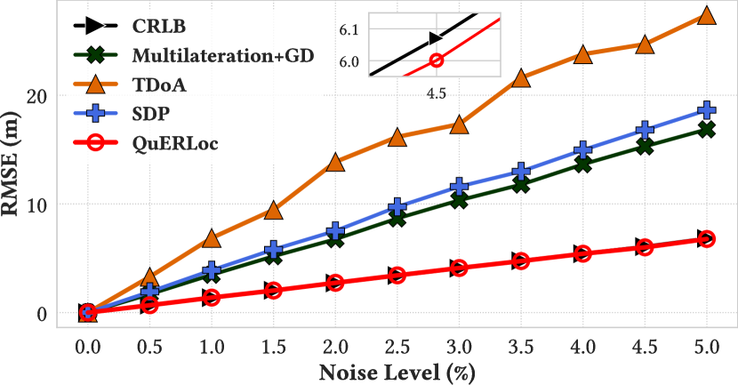
(a) RMSE, $m=3$

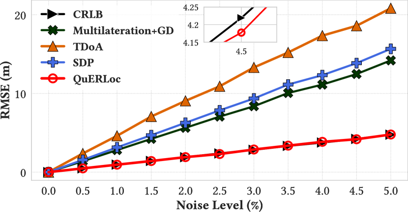
(b) RMSE, $m=4$

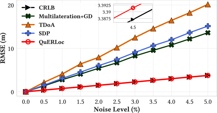
(c) RMSE, $m=5$

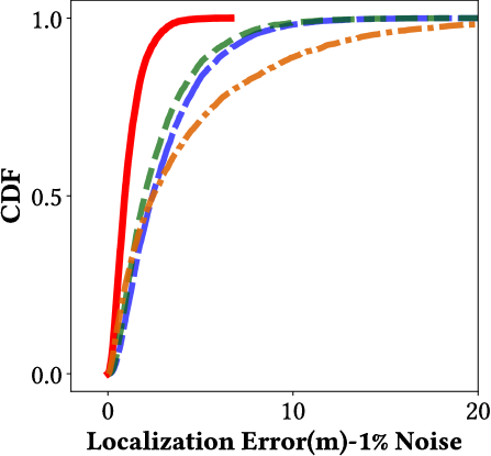
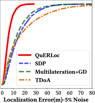
(d) CDF, $m=3$

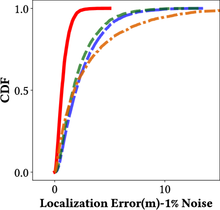
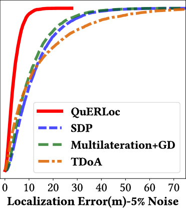
(e) CDF, $m=4$

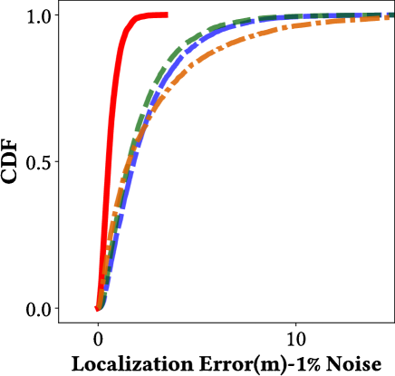
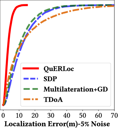
(f) CDF, $m=5$

Figure 6. Performance of QuERLoc and baselines with same anchor utilization. QuERLoc and all baseline methods conduct distance ranging with the same set of anchors.

7.2.2. Superiority of QuERLoc with Same Anchor Utilization

One may doubt that the superiority of QuERLoc merely originates from the full utilization of available anchors, as in the previous experiment, QuERLoc used twice as many anchor nodes as baselines. We address this question by doubling the quantity of distance ranging for baselines (i.e., they are conducting $2m$ rangings using the same anchors utilized by QuERLoc) while maintaining that of QuERLoc at $m$. As shown in Fig. 6, despite noticeable improvement in the performance of baselines, QuERLoc still largely outperforms them. As $m$ changes from $4$ to $5$, baselines only yield marginal accuracy improvement. QuERLoc achieves an RMSE of 27% compared to the best-performing baseline Multilateration + GD, as shown in Fig. 6c.

7.2.3. Case Study: Mimicking QuERLoc with Classical Ranging

One question might be raised naturally: Given that a distance combination analogous to (20) is central to the superiority of QuERLoc, is it possible to mimic such a ranging process with classical ranging, thus achieving the same localization accuracy? We explore the feasibility of this approach by conducting the following experiment: For each instance of QuER, classical ranging on each involved target-anchor distance $d_{i}$ is meanwhile conducted and combined. As for the systematic noise, we perturb corresponding readouts for QuERLoc and classical simulating system, denoted as QuERLoc-sim, as follows:

$$\textsc{QuERLoc}:\quad\widetilde{\lambda}_{k}=\left(1+\delta_{k}\right)\cdot\sum_{i\in I_{k}}w_{i,k}d_{i}^{2},\quad\delta_{k}\sim\mathcal{N}(0,\rho).$$

$$\textsc{QuERLoc}\text{-sim}:\quad\widetilde{\lambda}_{k}^{\prime}=\sum_{i\in I_{k}}w_{i,k}\left[d_{i}\cdot\left(1+\delta_{i}\right)\right]^{2},\quad\delta_{i}\sim\mathcal{N}(0,\rho).$$

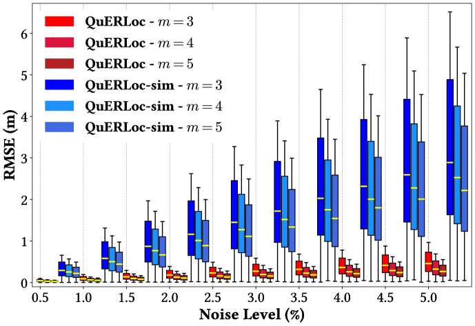
Figure 7. Comparison of QuERLoc and QuERLoc-sim with $m=3,4,5$ under non-zero noise levels $0.5\%$ to $5\%$. Each cluster of boxes corresponds to one noise level.

The localization performance under both settings is compared in Fig. 7. It be observed that the QuERLoc-sim suffers from evident deterioration in performance, as it doubles the quantity of ranging required compared to QuER under the designed probing scheme, and the noise is integrated into the system in a quadratic manner.

7.2.4. Time Complexity

Choosing localization methods involves a trade-off between accuracy and latency. Trilateration-based localization requires low running time but is highly sensible to noise, while conic relaxation and gradient-descent methods have no guarantee of instantaneous localization. As is illustrated in Tab. 2 the computational complexity and time consumption of several localization approaches when $\rho=5\%$, QuERLoc provides reliable localization with much more efficient computational requirements. On average, QuERLoc consumes only 2.4% of the time required by the most efficient baseline method Multilateration + GD.

Localization Methods	Time Complexity	Average Time Consumption (sec)
QuERLoc	${O}\left(d^{2}(m+d)\right)$	$3.27\times 10^{-4}$
SDP	${O}\left(\sqrt{d}(md^{2}+m^{\omega}+d^{\omega})\log(1/\alpha)\right)$   # state-of-the-art (Jiang et al., 2020)	$2.38\times 10^{-2}$
TDoA	${O}\left(d^{2}(m+d)+T_{{SOCP}}\right)$	$2.03\times 10^{-2}$
Multilateration+GD	${O}\left(d^{2}(m+d)+Md^{2}\right)$	$1.37\times 10^{-2}$

Table 2. Complexity and latency, $\rho=5\%$. $\alpha>0$ is the relative accuracy, $\omega$ is the exponent of matrix multiplication, and $M$ is the number of BFGS (default choice of gradient-descent search in cvxpy (Diamond and Boyd, 2016)) iterations. Asymptotic behaviour of $T_{{SOCP}}$ depends on the solver’s adaptive choice of problem reduction into various conic programming instances. When reduced to SDP, $T_{{SOCP}}={O}(\sqrt{d}(md^{2}+m^{\omega}+d^{\omega})\log(1/\alpha))$.

8. Conclusion

In this paper, we present QuERLoc, a novel localization approach that exploits the advantage of quantum-enhanced ranging realized by quantum metrology with entangled probes. We propose a new distance ranging model based on the quantum control theory and phase estimation by fine-tuning dynamics of quantum probes under two-level approximation, which we call QuER. We show that by a specially designed probe state, quantum-enhanced ranging can result in a convex optimization problem, which can be solved efficiently. Extensive simulations verify that QuERLoc significantly outperforms baseline approaches using classical ranging and saturates CRLB, demonstrating its superiority in both accuracy and latency. Our work provides a theoretical foundation for a potential application of quantum metrology in the field of range-based localization. We believe QuERLoc leads the research on localization with quantum resource and opens new directions to both fields of quantum computing and mobile computing.

References

- (1)
- Han (2000) 2000. Handbook of Semidefinite Programming. Springer US.
- Lec (2006) 2006. Lectures on Quantum Information. Wiley.
- Biswas et al. (2006) P. Biswas, T.-C. Liang, K.-C. Toh, Y. Ye, and T.-C. Wang. 2006. Semidefinite Programming Approaches for Sensor Network Localization With Noisy Distance Measurements. IEEE Transactions on Automation Science and Engineering 3, 4 (2006), 360–371.
- Buhrman et al. (2001) Harry Buhrman, Richard Cleve, John Watrous, and Ronald de Wolf. 2001. Quantum Fingerprinting. Phys. Rev. Lett. 87 (Sep 2001), 167902. Issue 16.
- Chintalapudi et al. (2010) Krishna Chintalapudi, Anand Padmanabha Iyer, and Venkata N. Padmanabhan. 2010. Indoor localization without the pain. In Proceedings of the sixteenth annual international conference on Mobile computing and networking (MobiCom’10). ACM, 293–304.
- Chiribella et al. (2004) G. Chiribella, G. M. D’Ariano, P. Perinotti, and M. F. Sacchi. 2004. Efficient Use of Quantum Resources for the Transmission of a Reference Frame. Phys. Rev. Lett. 93 (Oct 2004), 180503. Issue 18.
- Daems et al. (2013) D. Daems, A. Ruschhaupt, D. Sugny, and S. Guérin. 2013. Robust Quantum Control by a Single-Shot Shaped Pulse. Phys. Rev. Lett. 111 (Jul 2013). Issue 5.
- Dahl (2012) Joachim Dahl. 2012. Semidefinite optimization using MOSEK. ISMP, Berlin (2012).
- Diamond and Boyd (2016) Steven Diamond and Stephen Boyd. 2016. CVXPY: a python-embedded modeling language for convex optimization. J. Mach. Learn. Res. 17, 1 (jan 2016), 2909–2913.
- D’Alessandro (2021) Domenico D’Alessandro. 2021. Introduction to Quantum Control and Dynamics. Chapman and Hall/CRC.
- Giovannetti et al. (2001) Vittorio Giovannetti, Seth Lloyd, and Lorenzo Maccone. 2001. Quantum-enhanced positioning and clock synchronization. Nature 412, 6845 (July 2001), 417–419.
- Giovannetti et al. (2004) Vittorio Giovannetti, Seth Lloyd, and Lorenzo Maccone. 2004. Quantum-Enhanced Measurements: Beating the Standard Quantum Limit. Science 306, 5700 (Nov. 2004), 1330–1336.
- Giovannetti et al. (2006) Vittorio Giovannetti, Seth Lloyd, and Lorenzo Maccone. 2006. Quantum Metrology. Phys. Rev. Lett. 96 (Jan 2006), 010401. Issue 1.
- Giovannetti et al. (2011) Vittorio Giovannetti, Seth Lloyd, and Lorenzo Maccone. 2011. Advances in quantum metrology. Nature Photonics 5, 4 (March 2011), 222–229.
- Goyal et al. (2012) Sandeep K. Goyal, Subhashish Banerjee, and Sibasish Ghosh. 2012. Effect of control procedures on the evolution of entanglement in open quantum systems. Physical Review A 85, 1 (Jan. 2012).
- Grover (1997) Lov K. Grover. 1997. Quantum Mechanics Helps in Searching for a Needle in a Haystack. Phys. Rev. Lett. 79 (Jul 1997), 325–328. Issue 2.
- Itano et al. (1990) Wayne M. Itano, D. J. Heinzen, J. J. Bollinger, and D. J. Wineland. 1990. Quantum Zeno effect. Phys. Rev. A 41 (Mar 1990), 2295–2300. Issue 5.
- Jiang et al. (2020) Haotian Jiang, Tarun Kathuria, Yin Tat Lee, Swati Padmanabhan, and Zhao Song. 2020. A Faster Interior Point Method for Semidefinite Programming. In 2020 IEEE 61st Annual Symposium on Foundations of Computer Science (FOCS). IEEE.
- Koike-Akino et al. (2022) Toshiaki Koike-Akino, Pu Wang, and Ye Wang. 2022. Quantum Transfer Learning for Wi-Fi Sensing. In ICC 2022 - IEEE International Conference on Communications.
- Kotaru et al. (2015) Manikanta Kotaru, Kiran Joshi, Dinesh Bharadia, and Sachin Katti. 2015. SpotFi: Decimeter Level Localization Using WiFi. In Proceedings of the 2015 ACM Conference on Special Interest Group on Data Communication (SIGCOMM ’15). ACM, 269–282.
- Lin et al. (2013) Lanxin Lin, H.C. So, Frankie K.W. Chan, Y.T. Chan, and K.C. Ho. 2013. A new constrained weighted least squares algorithm for TDOA-based localization. Signal Processing 93, 11 (Nov. 2013), 2872–2878.
- Liu et al. (2012) Jie Liu, Bodhi Priyantha, Ted Hart, Heitor S. Ramos, Antonio A. F. Loureiro, and Qiang Wang. 2012. Energy efficient GPS sensing with cloud offloading. In Proceedings of the 10th ACM Conference on Embedded Network Sensor Systems (SenSys ’12). ACM, 85–98.
- Liu et al. (2003) Jie Liu, Biao Wu, and Qian Niu. 2003. Nonlinear Evolution of Quantum States in the Adiabatic Regime. Phys. Rev. Lett. 90 (May 2003), 170404. Issue 17.
- Liu et al. (2020) Li-Zheng Liu, Yu-Zhe Zhang, Zheng-Da Li, Rui Zhang, Xu-Fei Yin, Yue-Yang Fei, Li Li, Nai-Le Liu, Feihu Xu, Yu-Ao Chen, and Jian-Wei Pan. 2020. Distributed quantum phase estimation with entangled photons. Nature Photonics 15, 2 (Nov. 2020), 137–142.
- Mao et al. (2007) Guoqiang Mao, Barış Fidan, and Brian D.O. Anderson. 2007. Wireless sensor network localization techniques. Computer Networks 51, 10 (July 2007), 2529–2553.
- Mehboudi et al. (2019) Mohammad Mehboudi, Anna Sanpera, and Luis A Correa. 2019. Thermometry in the quantum regime: recent theoretical progress. Journal of Physics A: Mathematical and Theoretical 52, 30 (July 2019), 303001.
- Mitarai et al. (2023) Kosuke Mitarai, Kiichiro Toyoizumi, and Wataru Mizukami. 2023. Perturbation theory with quantum signal processing. Quantum 7 (May 2023), 1000.
- Nielsen and Chuang (2012) Michael A. Nielsen and Isaac L. Chuang. 2012. Quantum Computation and Quantum Information: 10th Anniversary Edition. Cambridge University Press.
- Pezzé and Smerzi (2014) Luca Pezzé and Augusto Smerzi. 2014. Quantum theory of phase estimation. arXiv preprint arXiv:1411.5164 (2014).
- Rai et al. (2012) Anshul Rai, Krishna Kant Chintalapudi, Venkata N. Padmanabhan, and Rijurekha Sen. 2012. Zee: zero-effort crowdsourcing for indoor localization. In Proceedings of the 18th annual international conference on Mobile computing and networking (Mobicom’12). ACM, 293–304.
- Rissanen (1996) Jorma J Rissanen. 1996. Fisher information and stochastic complexity. IEEE transactions on information theory 42, 1 (1996), 40–47.
- Shang et al. (2003) Yi Shang, Wheeler Ruml, Ying Zhang, and Markus P. J. Fromherz. 2003. Localization from mere connectivity. In Proceedings of the 4th ACM International Symposium on Mobile Ad Hoc Networking & Computing (MobiHoc ’03). ACM, 201–212.
- Shapiro and Brumer (2006) Moshe Shapiro and Paul Brumer. 2006. Quantum control of bound and continuum state dynamics. Physics Reports 425, 4 (March 2006), 195–264.
- Shokry and Youssef (2022) Ahmed Shokry and Moustafa Youssef. 2022. A Quantum Algorithm for RF-based Fingerprinting Localization Systems. In 2022 IEEE 47th Conference on Local Computer Networks (LCN). IEEE.
- So and Ye (2006) Anthony Man-Cho So and Yinyu Ye. 2006. Theory of semidefinite programming for Sensor Network Localization. Mathematical Programming 109, 2–3 (Sept. 2006), 367–384.
- Tseng (2007) Paul Tseng. 2007. Second‐Order Cone Programming Relaxation of Sensor Network Localization. SIAM Journal on Optimization 18, 1 (Jan. 2007), 156–185.
- Van Huffel and Zha (1993) Sabine Van Huffel and Hongyuan Zha. 1993. The total least squares problem. Elsevier, 377–408.
- Xiao et al. (2018) Fu Xiao, Lei Chen, Chaoheng Sha, Lijuan Sun, Ruchuan Wang, Alex X. Liu, and Faraz Ahmed. 2018. Noise Tolerant Localization for Sensor Networks. IEEE/ACM Transactions on Networking 26, 4 (Aug. 2018), 1701–1714.
- Xiao et al. (2014) Qingjun Xiao, Bin Xiao, Kai Bu, and Jiannong Cao. 2014. Iterative Localization of Wireless Sensor Networks: An Accurate and Robust Approach. IEEE/ACM Transactions on Networking 22, 2 (April 2014), 608–621.
- Yang et al. (2009b) Kehu Yang, Gang Wang, and Zhi-Quan Luo. 2009b. Efficient Convex Relaxation Methods for Robust Target Localization by a Sensor Network Using Time Differences of Arrivals. IEEE Transactions on Signal Processing 57, 7 (2009), 2775–2784.
- Yang et al. (2009a) Z. Yang, Y. Liu, and X.-Y. Li. 2009a. Beyond trilateration: On the localizability of wireless ad-hoc networks. In IEEE INFOCOM 2009. IEEE.
- Yu et al. (2009) Kegen Yu, Ian Sharp, and Y Jay Guo. 2009. Ground-based wireless positioning.
- Zhan and Gupta (2023) Caitao Zhan and Himanshu Gupta. 2023. Quantum Sensor Network Algorithms for Transmitter Localization. In 2023 IEEE International Conference on Quantum Computing and Engineering (QCE). IEEE.
- Zhang et al. (2022) Sheng Zhang, Yu-Kai Wu, Chang Li, Nan Jiang, Yun-Fei Pu, and Lu-Ming Duan. 2022. Quantum-Memory-Enhanced Preparation of Nonlocal Graph States. Phys. Rev. Lett. 128 (Feb 2022), 080501. Issue 8.
- Zhou and Shi (2008) Junyi Zhou and Jing Shi. 2008. RFID localization algorithms and applications—a review. Journal of Intelligent Manufacturing 20, 6 (Aug. 2008), 695–707.