Myopically Verifiable Probabilistic Certificates for Safe Control and Learning

Abstract

This paper addresses the design of safety certificates for stochastic systems, with a focus on ensuring long-term safety through fast real-time control. In stochastic environments, set invariance-based methods that restrict the probability of risk events in infinitesimal time intervals may exhibit significant long-term risks due to cumulative uncertainties/risks. On the other hand, reachability-based approaches that account for the long-term future may require prohibitive computation in real-time decision making. To overcome this challenge involving stringent long-term safety vs. computation tradeoffs, we first introduce a novel technique termed ‘probabilistic invariance’. This technique characterizes the invariance conditions of the probability of interest. When the target probability is defined using long-term trajectories, this technique can be used to design myopic conditions/controllers with assured long-term safe probability. Then, we integrate this technique into safe control and learning. The proposed control methods efficiently assure long-term safety using neural networks or model predictive controllers with short outlook horizons. The proposed learning methods can be used to guarantee long-term safety during and after training. Finally, we demonstrate the performance of the proposed techniques in numerical simulations.

I Introduction

Autonomous control systems must make safe control decisions in real-time and in the presence of uncertainties. Many techniques have been developed for deterministic systems with bounded uncertainties that can assure long-term safety with efficient computation [1, 2, 3]. These works often leverage set-invariance-based approaches [4, 5, 6] to transform long-term design specifications into sufficient myopic conditions. However, when a system has uncertainty with unbounded support (e.g., Gaussian noise), imposing set invariance on the state space for short-term future can no longer guarantee long-term safety. This is because even if the set invariance is satisfied with high probability at each time, uncertainty and risk may still accumulate over time.

Consequently, there are stringent trade-offs between ensuring safety for longer time horizons and reducing computation burden. For example, robust and stochastic barrier functions can be efficiently evaluated [7, 8, 9], but are insufficient to ensure long-term guarantees. On the other hand, conditions to control the probability of continuously satisfying set invariance conditions for a long period of time cannot be converted into myopic conditions. Similarly, reachability-based approaches (e.g., probabilistic reachability) often come with heavy computation to propagate uncertainties over time [10, 11, 12, 13, 14, 15]. These drawbacks pose significant challenges to control and learning methods for stochastic systems operating under latency-critical environments.

To address such challenges, in this paper, we propose a novel technique, termed probabilistic invariance. This technique is inspired by set invariance, but it defines invariance on the probability space, rather than on the state space. In particular, the probabilistic invariance technique allows one to efficiently evaluate probability about scenarios of long-term trajectories, such as probabilistic reachability. As such, this technique inherits the computational efficiency of the invariance-based approaches and the long-term guarantees of the reachability-based approaches. An infinitesimal future trajectory of a stochastic dynamical system provides little information about its future invariant sets on the state space. In comparison, our key insight is that its probabilistic analog, namely an infinitesimal future value of a long-term probability, does provide explicit computable information about invariant sets in the space of probability values. Building upon this insight, we characterize myopic conditions that can ensure conditions on long-term probability at all times.

Leveraging this feature, we first characterize myopic conditions for controlling two types of long-term probabilities to stay within a desirable range. The first type is the probability of forward invariance, which can be used to represent the probabilities of exiting certain sets (e.g., safe regions) within a time interval. The second type is the probability of forward convergence, which can be used to represent the probabilities of reaching or recovering to certain sets. For affine control systems, these conditions can be converted into linear control constraints, and thus can be easily integrated into convex/quadratic programs. Then, we apply the probabilistic invariance technique to safe control and learning problems. In the context of control, the proposed technique equips the nominal controllers, which are allowed to be neural networks and black-box, with long-term safety. In the context of learning, the proposed technique minimally changes the training procedures while ensuring the long-term safety of the control policies during and after training.

II Related Work

II-A Safety Certificate for Stochastic Systems

For deterministic systems with bounded uncertainties, previous work has developed various techniques for safe control (see review articles such as [3, 1, 16]), and the combination of set invariance and reachability-based techniques has also been studied in [17]. As this paper considers stochastic systems, our review below focuses on existing approaches for stochastic systems. We approximately classify these approaches into three main types based on their choice of tradeoffs: long-term safety with heavy computation; myopic safety with low computation; and long-term conservative safety with low computation.

Extensive literature exists that considers the distributions of the system state in the long term. Reachability-based techniques characterize the probability that states reach or avoid certain regions over a long period of time [10, 11, 12, 13, 14, 15], which are useful to evaluate the long-term safety of actions. However, these techniques often come with significant computational costs. The cause is two-fold. First, possible trajectories often scale exponentially with the length of the outlook time horizon. Second, rare events are more costly to sample and estimate than nominal events. Compared to these techniques, the proposed method only myopically evaluates the immediate future, and the safety constraints can be given in closed forms for affine control systems. These features help reduce real-time computation.

On the other hand, extensive work has been done to develop efficient controllers in latency-critical stochastic systems. Given the hard tradeoffs between time horizon vs. computation, many of these techniques impose set invariance on short-term or infinitesimal future states. For example, stochastic control barrier functions use a sufficient condition to ensure that the state moves within the tangent cone of the safe set on average [18]. The probabilistic barrier certificate ensures that conditions based on control barrier functions are met with high probability [8, 9]. The myopic nature of these methods achieves a significant reduction in computational cost. However, they can result in unsafe behaviors on a longer time horizon due to the accumulation of tail probabilities of hazardous events. In contrast, the proposed technique provides long-term safe probability guarantees by finding probabilistic invariance conditions that directly control the likelihood of accumulating tail events.

Other approaches, such as the barrier certificate, establish efficient methods to characterize safe action in a given time interval using conservative or approximate conditions. In these studies, probability bounds or martingale approximations are used to obtain sufficient conditions for long-term safety [19, 20, 21, 22, 23]. Many of such conditions can be integrated into convex optimization problems to synthesize safe controllers offline or verify control actions online. The controllers using these conditions often require less computation to design or execute. However, due to the approximate nature, control actions can be conservative and unnecessarily compromise performance. In contrast, the proposed techniques can use exact safe probability values (computed offline) and inform the probability of exposed risk in the event of infeasibility. These features allow control actions to be determined based on accurate probabilities without overconservatisms arising from overapproximation, and the aggressiveness of the performance to be systematically designed based on exposed risks.

II-B Integration with Learning-based Techniques

Here, we provide a brief summary of related work that integrates safety certificates (safety constraints) with control and reinforcement learning.

The safety certificates mentioned above (e.g., [3, 18, 8, 9]) are commonly used to certify or modify nominal controllers. The nominal controllers are often allowed to be either black-box models or represented by neural networks. As stated above, in stochastic systems, when safety certificates are formulated using myopic conditions, they do not necessarily ensure long-term safety. When they are constructed based on approximations or designed to be safe in worst-case uncertainties, the system performance may degrade significantly as the size of uncertainties increases. On the other hand, the proposed certificate can be used similarly to existing safety certificates but ensures long-term safety using myopic controllers and exhibits graceful degradation for increasing uncertainties. Alternatively, safety considerations can be captured in rewards and constraints in model predictive control (MPC) [25, 26]. When safety specifications for future states are directly expressed in the reward and constraint functions, the MPC outlook time horizon needs to cover such future states. In comparison, the proposed technique can be used to construct MPC constraints in a way that ensures safety for a longer period than the MPC outlook horizon.

There exists extensive literature on safe reinforcement learning, as reviewed in [27, 28]. Some approaches account for safety specifications in rewards or constraints [29, 30, 31, 32, 33] or design/learn certain functions related to safe conditions [34, 35, 35, 36, 37, 38]. Examples of these functions are control barrier functions [34], safety index [35], barrier certificate [36], rewards and constraints [37, 38]. These methods aim to learn optimal and safe policies but may not guarantee safety in the initial learning phase. Other approaches impose additional structures on control policies [39, 40, 41]. For example, safety filters (e.g., Lyapunov conditions, control barrier functions, typically defined by prior knowledge of system models) are attached to learning-based controllers, and can often ensure safety or stability for deterministic systems or bounded uncertainties. Similarly, the proposed technique can be used to construct a safety filter for learning-based controllers. When used as a safety filter, it can control, both during and after training, the probability of forward invariance for a given duration or forward convergence within a given horizon for stochastic nonlinear systems.

III Preliminary

Let $\mathbb{R}$, $\mathbb{R}_{+}$, $\mathbb{R}^{n}$, and $\mathbb{R}^{m\times n}$ be the set of real numbers, the set of non-negative real numbers, the set of $n$-dimensional real vectors, and the set of $m\times n$ real matrices, respectively. Let $x[k]$ be the $k$-th element of vector $x$. Let $X_{a:b}$ denote the set $\{X_{i}:i\in\{a,a+1,\cdots,b\}\}$, where $a,b\in\mathbb{Z}$ and $a\leq b$. Let $f:{\mathcal{X}}\rightarrow{\mathcal{Y}}$ represent that $f$ is a mapping from space ${\mathcal{X}}$ to space ${\mathcal{Y}}$. Let $\mathbb{1}({\mathcal{E}})$ be an indicator function, which takes $1$ when condition ${\mathcal{E}}$ holds and $0$ otherwise. Let $\mathbf{0}_{m\times n}$ be an $m\times n$ matrix with all entries $0$. Given events ${\mathcal{E}}$ and ${\mathcal{E}}_{c}$, let $\mathbb{P}({\mathcal{E}})$ be the probability of ${\mathcal{E}}$ and $\mathbb{P}({\mathcal{E}}|{\mathcal{E}}_{c})$ be the conditional probability of ${\mathcal{E}}$ given the occurrence of ${\mathcal{E}}_{c}$. Given random variables $X$ and $Y$, let $\mathbb{E}[X]$ be the expectation of $X$ and $\mathbb{E}[X|Y=y]$ be the conditional expectation of $X$ given $Y=y$. We use upper-case letters (e.g., $Y$) to denote random variables and lower-case letters (e.g., $y$) to denote their specific realizations.

Definition 1 (Infinitesimal Generator).

The infinitesimal generator $A$ of a stochastic process $\{Y_{t}\in\mathbb{R}^{n}\}_{t\in\mathbb{R}_{+}}$ is

$$AF(y)=\lim_{h\to 0}\frac{\mathbb{E}[F(Y_{h})|Y_{0}=y]-F(y)}{h}$$ (1)

whose domain is the set of all functions $F:\mathbb{R}^{n}\rightarrow\mathbb{R}$ such that the limit of (1) exists for all $y\in\mathbb{R}^{n}$.

IV Problem Statement

Here, we introduce the control system in subsection IV-A, define the safety specification in subsection IV-B, and state the controller design goals in subsection IV-C.

IV-A Control System Description

We consider a time-invariant control-affine stochastic control and dynamical system. The system dynamics is given by the stochastic differential equation (SDE)

$$dX_{t}=\left(f(X_{t})+g(X_{t})U_{t}\right)dt+\sigma(X_{t})dW_{t},$$ (2)

where $X_{t}\in\mathcal{X}\subseteq\mathbb{R}^{n}$ is the system state, $U_{t}\in\mathcal{U}\subseteq\mathbb{R}^{m}$ is the control input, and $W_{t}\in\mathbb{R}^{\xi}$ captures the system uncertainties. Here, $X_{t}$ can include both the controllable states of the system and the uncontrollable environmental variables such as moving obstacles. We assume that $W_{t}$ is the standard Wiener process with $0$ initial value, i.e., $W_{0}=0$. The value of $\sigma(X_{t})$ is determined based on the size of uncertainty in unmodeled dynamics, environmental variables and noise.

The control action $U_{t}$ is determined at each time by the control policy. We assume that accurate information of the system state can be used by the control policy. The control policy is composed of a nominal controller and additional modification scheme to ensure the safety specifications illustrated in subsection IV-B. The nominal controller is represented by

$$U_{t}=N(X_{t}),$$ (3)

where function $N$ lies in a class of stochastic or deterministic functions mapping $\mathcal{X}$ to $\mathcal{U}$, i.e., $N\in\mathcal{N}_{s}\cup\mathcal{N}_{d}$. Here, $\mathcal{N}_{s}$ denotes the class of stochastic functions, $\mathcal{N}_{d}$ denotes the class of stochastic functions, and we use $\mathcal{N}$ to denote the function class when it can be either. The design of $N$ does not necessarily account for the safety specifications defined below and can be represented by neural networks. To adhere to the safety specifications, the output of the nominal controller is then modified by another scheme. The overall control policy involving the nominal controller and the modification scheme is represented by

$$U_{t}=N^{\prime}(X_{t},L_{t},T_{t}),$$ (4)

where $N^{\prime}:\mathbb{R}^{n}\times\mathbb{R}\times\mathbb{R}\rightarrow\mathbb{R}^{m}$ is a mapping from the current state $X_{t}$, safety margin $L_{t}$, and time horizon $T_{t}$ to the current control action $U_{t}$. The formal definition of $L_{t}$ and $T_{t}$ will be given later in the section. The policy of the form (4) assumes that the decision rule is time-invariant. This policy is also assumed to be memory-less in the sense that it does not use the past history of the state $\{X_{\tau}\}_{\tau<t}$ to produce the control action $U_{t}$. The assumption for memory-less controller is reasonable because the state evolution $dX_{t}$ of system (2) only depends on the current system state $X_{t}$ as $f(X_{t})$, $g(X_{t})$, and $\sigma(X_{t})$ are time-invariant functions of the system state. We restrict ourselves to the settings when $f$, $g$, $\sigma$, $N$, and $N^{\prime}$ have sufficient regularity conditions such that the closed loop system of (2) and (4) has unique strong solutions. Conditions required to have a unique strong solution can be found in [42, Chapter 1], [43, Chapter II.7] and references therein.

The safe region of the state is specified by the zero super level set of a continuously differentiable barrier function $\phi(x):\mathbb{R}^{n}\rightarrow\mathbb{R}$, i.e.,

$${\mathcal{C}}(0)=\left\{x\in\mathbb{R}^{n}:\phi(x)\geq 0\right\}.$$ (5)

We use

$${\mathcal{C}}(L):=\left\{x\in\mathbb{R}^{n}:\phi(x)\geq L\right\}$$ (6)

to denote the $L$-super level set of $\phi$ (the set with safety margin $L$). Accordingly, we use $\text{int}\,{{\mathcal{C}}(L)}=\{x\in\mathbb{R}^{n}:\phi(x)>L\}$ to denote the interior of the safe set, ${\mathcal{C}}(L)^{c}=\{x\in\mathbb{R}^{n}:\phi(x)<L\}$ to denote the unsafe set, $\partial{\mathcal{C}}(L)=\{x\in\mathbb{R}^{n}:\phi(x)=L\}$ to denote the boundary of $L$ super level set.

IV-B Safety Specifications

We consider two types of safety specifications: forward invariance and forward convergence. The two types are used to define the following four types of safety-related probabilities.

IV-B1 Forward Invariance

Long-term safety and long-term avoidance are expressed in the forms of forward invariance conditions. The forward invariance property refers to the system’s ability to keep its state within a set when the state originated from the set. The probabilistic forward invariance to a set ${\mathcal{C}}(L_{t})$ can be quantified using

$$\mathbb{P}\left(\,X_{\tau}\in{\mathcal{C}}(L_{t}),\forall\tau\in[t,t+T_{t}]\ |\ X_{t}=x\,\right)$$ (7)

for some time interval $[t,t+T_{t}]$ conditioned on an initial condition $x\in{\mathcal{C}}(L)$. Probability (7) can be computed from the distribution of the following two random variables:

$$\Phi_{x}(T_{t}) :=\inf\{\phi(X_{\tau})\in\mathbb{R}:\tau\in[0,T_{t}],X_{0}=x\},$$ (8)

$$\Gamma_{x}(L_{t}) :=\inf\{\tau\in\mathbb{R}_{+}:\phi(X_{\tau})<L_{t},X_{0}=x\}.$$ (9)

Here, $\Phi_{x}(T_{t})$ is the worst-case safety margin from the boundary of the safe set $\partial{\mathcal{C}}(0)$ during $[0,T_{t}]$, and $\Gamma_{x}(L_{t})$ is the time when the system exit from ${\mathcal{C}}(L_{t})$ for the first time. We can rewrite (7) using the two random variables (8) and (9) as

$$\mathbb{P}\left(\,X_{\tau}\in{\mathcal{C}}(L_{t}),\forall\tau\in[t,t+T_{t}]\ |\ X_{t}=x\,\right)$$ (10)

$$=\>\mathbb{P}\left(X_{\tau}\in{\mathcal{C}}(L_{t}),\forall\tau\in[0,T_{t}]\ |\ X_{0}=x\right)$$ (11)

$$=\>\mathbb{P}(\Phi_{x}(T_{t})\geq L_{t})$$ (12)

$$=\>\mathbb{P}(\Gamma_{x}(L_{t})>T_{t})=\>1-\mathbb{P}(\Gamma_{x}(L_{t})\leq T_{t}).$$ (13)

Here, equality (11) holds due to the time-invariant nature of the system and control policies.

Type 1: long-term safety is defined using forward invariance assuming the continued use of the current (nominal) controller (3) given $X_{t}\in{\mathcal{C}}(L_{t})$ at time $t$. Its probability is given by

$$P_{1}(x,L,T,\phi):=\mathbb{P}\{X_{\tau}\in{\mathcal{C}}(L),\forall\tau\in[t,t+T]\mid X_{t}=x\},$$ (14)

where the probability is evaluated assuming $U_{\tau}=N(X_{\tau}),\forall\tau\in[t,t+T]$.

Type 2: long-term avoidance is defined using forward invariance assuming the future control action can be modified given $X_{t}\in{\mathcal{C}}(L)$ at time $t$. The long-term avoidance is quantified by

$$P_{2}(x,L,T,\phi):=\sup_{N\in\mathcal{N}}\mathbb{P}\{X_{\tau}\in{\mathcal{C}}(L),$$ (15)

$$\qquad\qquad\forall\tau\in[t,t+T]\mid X_{t}=x\},$$

where the probability is evaluated assuming $U_{\tau}=N(X_{\tau}),\forall\tau\in[t,t+T]$. The probability of long-term safety will be used to measure the likelihood of remaining safe under the current controller, and the probability of long-term avoidance will be used to measure the possibility to avoid unsafe events, independently from the current choice of the control policy.

IV-B2 Forward Convergence

Finite-time eventuality and reachability are expressed in the forms of forward convergence conditions (i.e., having the state converge to a set ${\mathcal{C}}$ within $T_{t}$). The forward convergence property indicates the system’s capability for its state to enter a set when the state originated from outside the set. This probabilistic forward convergence can be quantified using

$$\mathbb{P}\left(\,\exists\tau\in[t,t+T_{t}]\text{ s.t. }X_{\tau}\in{\mathcal{C}}(L_{t})\ |\ X_{t}=x\,\right)$$ (16)

for some time interval $[t,t+T_{t}]$ conditioned on an initial condition $x\in{\mathcal{C}}(L_{t})^{c}$. Similar to the case of forward invariance, probability (16) can also be computed from the distribution of the following two random variables:eq:rv-intro

$$\Theta_{x}(T_{t}) :=\sup\{\phi(X_{\tau})\in\mathbb{R}:\tau\in[0,T_{t}],X_{0}=x\},$$ (17)

$$\Psi_{x}(L_{t}) :=\inf\{\tau\in\mathbb{R}_{+}:\phi(X_{\tau})\geq L_{t},X_{0}=x\}.$$ (18)

Here, $\Theta_{x}(T_{t})$ indicates the distance to the boundary of the safe set $\partial{\mathcal{C}}(0)$, and $\Psi_{x}(L_{t})$ is the duration for the state to enter the set ${\mathcal{C}}(L_{t})$ for the first time. We can also rewrite (16) using the two random variables (17) and (18) as

$$\mathbb{P}\left(\,\exists\tau\in[t,t+T_{t}]\text{ s.t. }X_{\tau}\in{\mathcal{C}}(L_{t})\ |\ X_{t}=x\,\right)$$ (19)

$$=\>\mathbb{P}\left(\ \exists\tau\in[0,T_{t}]\text{ s.t. }X_{\tau}\in{\mathcal{C}}(L_{t})\ |\ X_{0}=x\ \right)$$ (20)

$$=\>\mathbb{P}(\Theta_{x}(T_{t})\geq L_{t})$$ (21)

$$=\>\mathbb{P}(\Psi_{x}(L_{t})\leq T_{t}).$$ (22)

Type 3: finite-time eventuality is defined using forward convergence assuming continued use of the current (nominal) controller (3) where it is given $X_{t}\notin{\mathcal{C}}(L)$ at time $t$. Its probability is given by

$$P_{3}(x,L,T,\phi):=\mathbb{P}\{X_{\tau}\in{\mathcal{C}}(L)$$ (23)

$$\quad\text{ for some }\tau\in[t,t+T]\mid X_{t}=x\},$$

where the probability is evaluated assuming $U_{\tau}=N(X_{\tau}),\forall\tau\in[t,t+T]$.

Type 4: finite-time reachability is defined using forward convergence assuming the future control action can be modified given $X_{t}\notin{\mathcal{C}}(L_{t})$ at time $t$. The finite-time reachability is quantified by

$$P_{4}(x,L,T,\phi):=\sup_{N\in\mathcal{N}}\mathbb{P}\{X_{\tau}\in{\mathcal{C}}(L)$$ (24)

$$\quad\text{ for some }\tau\in[t,t+T]\mid X_{t}=x\},$$

where the probability is evaluated assuming $U_{\tau}=N(X_{\tau}),\forall\tau\in[t,t+T]$. The finite-time eventuality will be used to measure the likelihood of reaching the desired states under the current controller and the finite-time reachability will be used to measure of the system’s capability to do so.

IV-C Design Goals

This objective of this paper is to ensure either long-term safety/avoidance or finite-time eventuality/reachability. The objective is mathematically defined as follows. For simplicity of notations, we define the following probability

$$P(x,L,T,\phi):=\begin{cases}P_{1}(x,L,T,\phi),\quad\text{for type 1}\\ P_{2}(x,L,T,\phi),\quad\text{for type 2}\\ P_{3}(x,L,T,\phi),\quad\text{for type 3}\\ P_{4}(x,L,T,\phi),\quad\text{for type 4}\end{cases}$$ (25)

The long term safety condition we aim to ensure is defined as

$$\mathbb{E}\left[P(X_{t},L_{t},T_{t},\phi)\right]\geq 1-\epsilon,\quad\forall t>0$$ (26)

where $\epsilon\in(0,1)$ is the pre-specified risk tolerance. The expectation (26) is taken over the distribution of $X_{t}$ and the future trajectories $\{X_{\tau}\}_{\tau\in(t,t+T_{t}]}$ conditioned on the initial distribution of $X_{0}$. The distribution of $X_{t}$ is generated based on the closed-loop system of (2) and (4), whereas the distribution of $\{X_{\tau}\}_{\tau\in(t,t+T_{t}]}$ are allowed to be defined in two different ways based on the design choice: the closed-loop system of (2) and (3) or the closed-loop system of (2) and (4).

The physical meaning of the objective (26) is that we want the probability of long-term safety at each time step to be greater than a pre-specified threshold. For example, when (25) is defined for type 1, we have

$$\mathbb{E}\left[P(X_{t},L_{t},T_{t},\phi)\right]=\mathbb{P}\left(X_{\tau}\in{\mathcal{C}}(L_{t}),\forall\tau\in[t,t+T_{t}]\right).$$ (27)

We consider either fixed time horizon problem or receding time horizon problem. In the fixed time horizon problem, safety is evaluated at each time $t$ for a time interval $[t,t+H]$ of fixed length. In the receding time horizon problem, we evaluate, at each time $t$, safety only for the remaining time $[t,H]$ given a fixed horizon. The outlook time horizon for each case is given by

$$T_{t} =\begin{cases}H-t,&\text{for fixed time horizon,}\\ H,&\text{for receding time horizon.}\end{cases}$$ (28)

The safety margin is assumed to be either fixed or time varying. Fixed margin refers to when the margin remains constant at all time, i.e., $L_{t}=\ell$. For time-varying margin, we consider the margin $L_{t}$ that evolves according to

$$dL_{t}/dt=f_{\ell}(L_{t}),\ L_{0}=\ell,$$ (29)

for some continuously differentiable function $f_{\ell}$. This representation includes fixed margin by setting $f_{\ell}(L_{t})\equiv 0$. The values of $T_{t}$ and $\{L_{t}\}_{t\in\mathbb{R}^{+}}$ are determined based on the design choice.

V Probabilistic Safety Certificate

Here, we present a sufficient condition to achieve the safety requirements in subsection V-A. Then we provide efficient computation methods to calculate the safety condition in subsection V-B. Finally, we propose two safe control strategies and conclude the overall framework in subsection V-C.

Before presenting these results, we first define a few notations. To capture the time-varying nature of $T_{t}\text{ and }L_{t}$, we augment the state space as

$$Z_{t}:=\begin{bmatrix}T_{t}\\ L_{t}\\ \phi(X_{t})\\ X_{t}\end{bmatrix}\in\mathbb{R}^{n+3}.$$ (30)

The dynamics of $Z_{t}$ satisfies the following SDE:

$$dZ_{t}=(\tilde{f}(Z_{t})+\tilde{g}(Z_{t})U_{t})dt+\tilde{\sigma}(Z_{t})dW_{t}.$$ (31)

Here, $\tilde{f}$, $\tilde{g}$, and $\tilde{\sigma}$ are defined to be

$$\tilde{f}(Z_{t}) :=\begin{bmatrix}f_{T}\\ f_{\ell}(L_{t})\\ f_{\phi}(X_{t})\\ f(X_{t})\end{bmatrix}\in\mathbb{R}^{(n+3)},$$ (32)

$$\tilde{g}(Z_{t}) :=\begin{bmatrix}\mathbf{0}_{2\times m}\\ {\mathcal{L}}_{g}\phi(X_{t})\\ g(X_{t})\end{bmatrix}\in\mathbb{R}^{(n+3)\times m},$$ (33)

$$\tilde{\sigma}(Z_{t}) :=\begin{bmatrix}\mathbf{0}_{2\times\xi}\\ {\mathcal{L}}_{\sigma}\phi(X_{t})\\ \sigma(X_{t})\end{bmatrix}\in\mathbb{R}^{(n+3)\times\xi}.$$ (34)

In (32), the scalar $f_{T}$ is given by

$$f_{T} :=\begin{cases}0,&\text{in fixed time horizon,}\\ -1,&\text{in receding time horizon,}\end{cases}$$ (35)

the function $f_{\ell}$ is given by (29), and the function $f_{\phi}$ is given by

$$f_{\phi}(X_{t}) :={\mathcal{L}}_{f}\phi(X_{t})+\frac{1}{2}\text{tr}\big{(}\left[\sigma(X_{t})\right]\left[\sigma(X_{t})\right]^{\intercal}\operatorname{Hess}{\phi}(X_{t})\big{)}.$$ (36)

Remark 1.

The Lie derivative of a function $\phi(x)$ along the vector field $f(x)$ is denoted as ${\mathcal{L}}_{f}\phi(x)=f(x)\cdot\nabla\phi(x)$. The Lie derivative $({\mathcal{L}}_{g}\phi(x))$ along a matrix field $g(x)$ is interpreted as a row vector such that $\left({\mathcal{L}}_{g}\phi(x)\right)u=\left(g(x)u\right)\cdot\nabla\phi(x)$.

V-A Conditions to Assure Safety

We consider the following probabilistic quantity:

$$\mathbf{F}(Z_{t}):=P(X_{t},L_{t},T_{t},\phi),$$ (37)

where the probability is taken over the same distributions of $\{X_{\tau}\}_{\tau\in[t,T_{t}]}$ that are used in the safety requirement (26). The values of $T_{t}$ and $L_{t}$ (known and deterministic) are defined in 28 and 29 depending on the design choice of receding/fixed time-horizon and fixed/varying margin.

Additionally, we define the mapping $D_{\mathbf{F}}:\mathbb{R}^{n+3}\times\mathbb{R}^{m}\rightarrow\mathbb{R}$ as

$$\begin{split}D_{\mathbf{F}}(Z_{t},U_{t}):=&\ {\mathcal{L}}_{\tilde{f}}\mathbf{F}(Z_{t})+\left({\mathcal{L}}_{\tilde{g}}\mathbf{F}(Z_{t})\right)U_{t}\\ &+\frac{1}{2}\text{tr}\left(\left[\tilde{\sigma}(Z_{t})\right]\left[\tilde{\sigma}(Z_{t})\right]^{\intercal}\operatorname{Hess}{\mathbf{F}}(Z_{t})\right).\end{split}$$ (38)

From Itô’s Lemma, the mapping (38) essentially evaluates the value of the infinitesimal generator of the stochastic process $Z_{t}$ acting on $\mathbf{F}$: i.e., $A\mathbf{F}(Z_{t})=D_{\mathbf{F}}(Z_{t},U_{t})$ when the control action $U_{t}$ is used.

We propose to constrain the control action $U_{t}$ to satisfy the following condition at all time $t$:

$$D_{\mathbf{F}}(Z_{t},U_{t})\geq-\alpha\left(\mathbf{F}(Z_{t})-(1-\epsilon)\right).$$ (39)

Here, $\alpha:\mathbb{R}\rightarrow\mathbb{R}$ is assumed to be a monotonically-increasing, concave or linear function that satisfies $\alpha(0)\leq 0$. From (38), condition (39) is affine in $U_{t}$. This property allows us to integrate condition (39) into a convex/quadratic program. Note that (39) is a forward invariance condition on probability, while typical control barrier function (CBF) based methods perform forward invariance on state space. The advantage of imposing forward invariance on the probability space is that long-term safety can be ensured. In contrast, directly imposing forward invariance on the barrier function $\phi$ can not guarantee long-term safety (see Fig. 1 for comparison results).

Theorem 1.

Consider the closed-loop system of $\eqref{eq:x_trajectory}$ and (4), where $f$, $g$, $\sigma$, $N$, and $N^{\prime}$ are assumed to have sufficient regularity conditions. Assume that $\mathbf{F}(z)$ in 37 is a continuously differentiable function of $z\in\mathbb{R}^{n+3}$ and $\mathbb{E}[\mathbf{F}(Z_{t})]$ is differentiable in $t$. If system (2) originates at $X_{0}=x$ with $\mathbf{F}(z)>1-\epsilon$, and the control action satisfies (39) at all time, then the following condition holds:

$$\mathbb{E}\left[\mathbf{F}(Z_{t})\right]\geq 1-\epsilon$$ (40)

for all time $t\in\mathbb{R}_{+}$.

Proof (theorem 1).

First, we show that

$$\mathbb{E}[\mathbf{F}(Z_{\tau})]\leq 1-\epsilon$$ (41)

implies

$$\mathbb{E}\left[\alpha\left(\mathbf{F}(Z_{\tau})-(1-\epsilon)\right)\right]\leq 0,$$ (42)

where we let $\tau$ be the time when (41) holds. We first define the events $D_{i}$ and a few variables $v_{i},q_{i},\text{ and }\delta_{i}$, $i\in\{0,1\}$, as follows:

$$D_{0} =\left\{\mathbf{F}(Z_{\tau})<1-\epsilon\right\},$$ (43)

$$D_{1} =\left\{\mathbf{F}(Z_{\tau})\geq 1-\epsilon\right\},$$ (44)

$$v_{0} =\mathbb{E}\left[\mathbf{F}(Z_{\tau})\mid D_{0}\right]=1-\epsilon-\delta_{0},$$ (45)

$$v_{1} =\mathbb{E}\left[\mathbf{F}(Z_{\tau})\mid D_{1}\right]=1-\epsilon+\delta_{1},$$ (46)

$$q_{0} =\mathbb{P}(D_{0}),$$ (47)

$$q_{1} =\mathbb{P}(D_{1}).$$ (48)

The left hand side of 41 can then be written as

$$\mathbb{E}[\mathbf{F}(Z_{\tau})] =\mathbb{E}\left[\mathbf{F}(Z_{\tau})\mid D_{0}\right]\mathbb{P}(D_{0})+\mathbb{E}\left[\mathbf{F}(Z_{\tau})\mid D_{1}\right]\mathbb{P}(D_{1})$$

$$=v_{0}q_{0}+v_{1}q_{1}.$$ (49)

From

$$\begin{aligned} \mathbb{E}\left[\mathbf{F}(Z_{\tau})\mid D_{0}\right]&<1-\epsilon,\\ \mathbb{E}\left[\mathbf{F}(Z_{\tau})\mid D_{1}\right]&\geq 1-\epsilon,\end{aligned}$$ (50)

we obtain

$$\delta_{0}\geq 0\quad\text{and}\quad\delta_{1}\geq 0.$$ (51)

Moreover, $\{q_{i}\}_{i\in\{0,1\}}$ satisfies

$$\mathbb{P}(D_{0})+\mathbb{P}(D_{1})=q_{0}+q_{1}=1.$$ (52)

Combining (41) and (49) gives

$$v_{0}q_{0}+v_{1}q_{1}\leq 1-\epsilon.$$ (53)

Applying 45 and 46 to 53 gives

$$\left(1-\epsilon-\delta_{0}\right)q_{0}+\left(1-\epsilon+\delta_{1}\right)q_{1}\leq 1-\epsilon,$$ (54)

which, combined with (52), yields

$$\delta_{1}q_{1}-\delta_{0}q_{0}\leq 0.$$ (55)

On the other hand, we have

$$\mathbb{E}\left[\alpha\left(\mathbf{F}(Z_{\tau})-(1-\epsilon)\right)\right]$$

$$\ \ \ \ \ =\ \mathbb{P}(D_{0})\left(\mathbb{E}\left[\alpha\left(\mathbf{F}(Z_{\tau})-(1-\epsilon)\right)\mid D_{0}\right]\right)$$

$$\ \ \ \ \ \ \ \ +\mathbb{P}(D_{1})\left(\mathbb{E}\left[\alpha\left(\mathbf{F}(Z_{\tau})-(1-\epsilon)\right)\mid D_{1}\right]\right)$$ (56)

$$\ \ \ \ \ =\ q_{0}\left(\mathbb{E}\left[\alpha\left(\mathbf{F}(Z_{\tau})-(1-\epsilon)\right)\mid D_{0}\right]\right)$$

$$\ \ \ \ \ \ \ \ +q_{1}\left(\mathbb{E}\left[\alpha\left(\mathbf{F}(Z_{\tau})-(1-\epsilon)\right)\mid D_{1}\right]\right)$$ (57)

$$\ \ \ \ \ \leq\ q_{0}\left(\alpha\left(\mathbb{E}\left[\mathbf{F}(Z_{\tau})-(1-\epsilon)\mid D_{0}\right]\right)\right)$$

$$\ \ \ \ \ \ \ \ +q_{1}\left(\alpha\left(\mathbb{E}\left[\mathbf{F}(Z_{\tau})-(1-\epsilon)\mid D_{1}\right]\right)\right)$$ (58)

$$\ \ \ \ \ =\ q_{0}\left(\alpha\left(-\delta_{0}\right)\right)+q_{1}\left(\alpha\left(\delta_{1}\right)\right)$$ (59)

$$\ \ \ \ \ \leq\ \alpha\left(-q_{0}\delta_{0}+q_{1}\delta_{1}\right)$$ (60)

$$\ \ \ \ \ \leq\ 0.$$ (61)

Here, (57) is due to (47) and (48); (58) is obtained from Jensen’s inequality [45] for concave function $\alpha$; (59) is based on (45) and (46); (60) is given by the assumptions on function $\alpha$; and (61) is due to (55). Thus, we showed that (41) implies (42).

Using Dynkin’s formula, given a time-invariant control policy, the sequence $\mathbb{E}[\mathbf{F}(Z_{t})]$ takes deterministic value over time where the dynamics is given by

$$\frac{d}{d\tau}\mathbb{E}[\mathbf{F}(Z_{\tau})]=\mathbb{E}[A\mathbf{F}(Z_{\tau})].$$ (62)

Condition (39) implies

$$\mathbb{E}[A\mathbf{F}(Z_{\tau})]\geq-\mathbb{E}\left[\alpha\left(\mathbf{F}(Z_{\tau})-\left(1-\epsilon\right)\right)\right].$$ (63)

Therefore, we have

$$\frac{d}{d\tau}\mathbb{E}[\mathbf{F}(Z_{\tau})]\geq 0\quad\text{whenever $\mathbb{E}[\mathbf{F}(Z_{\tau})]\leq 1-\epsilon$}.$$ (64)

This condition implies

$$\mathbb{E}[\mathbf{F}(Z_{t})]\geq 1-\epsilon\quad\text{for all $t\in\mathbb{R}_{+}$.}$$ (65)

due to Lemma 1, which is given below. ∎

Lemma 1.

Let $y\colon\mathbb{R}_{+}\to\mathbb{R}$ be a real-valued differentiable function that satisfies

$$\frac{d}{dt}y_{t}\geq 0\quad\text{whenever $y_{t}\leq L$}.$$ (66)

Additionally, we assume $y_{0}>L$. Then

$$y_{t}\geq L\quad\text{for all $t\in\mathbb{R}_{+}$.}$$ (67)

Proof (lemma 1).

Suppose there exists $b\in\mathbb{R}_{+}$ such that $y_{b}<L$. By the intermediate value theorem, there exists $a\in(0,b)$ such that $y_{a}=L$, and $y_{t}<L$ for all $t\in(a,b]$. Next, by the mean value theorem, there exists $\tau\in(a,b)$ such that $(dy_{t}/dt)|_{t=\tau}=(y_{b}-y_{a})/(b-a)<0$. This contradicts condition (66). ∎

V-B Efficient Computation of Long-term Probabilities

In this section, we provide computation methods to calculate the probability of the safety-related events. While the proposed safe control technique works for both stochastic and deterministic control policies, we here present computation methods for the cases of deterministic policies which are more commonly considered. Before introducing computation methods for controller implementation, we first consider a discretized version of dynamical system (2) for sampling time $\Delta t$:

$$X_{t+\Delta t}=F_{d}(X_{t},U_{t},W_{t}),$$ (68)

where $F_{d}$ is the discrete-time system dynamics. We also consider a discrete time horizon $T_{d}=\frac{T}{\Delta t}$. For simplicity, with a slight abuse of notation, we use $X_{k}$ to denote the system state evaluated at time $k\Delta t$ in this subsection.

V-B1 Long-term safety and finite time eventuality

Importance sampling techniques provide us with efficient computation methods to calculate the probabilities when the nominal control is fixed [46, 47]. Assume $N\in\mathcal{N}_{d}$ is the nominal controller that we are interested in, and $N_{s}\in\mathcal{N}_{d}$ is another controller that we have sampled data with. Let $\mathcal{P}_{N}$ denote the measure over the classical Wiener space $\Omega=C([0,T];\mathbb{R}^{n})$ induced by the dynamics (68) with $U_{k}=N(X_{k})$, and $\mathcal{P}_{N_{s}}$ denote the measure associated with the process with $U_{k}=N_{s}(X_{k})$. Note that $N_{s}$ can output zero values where the process is uncontrolled. Let $\tilde{U}_{k}=N(X_{k})-N_{s}(X_{k})$ denote the difference between the nominal controller and the sampled controller, where $X_{k}$ is the state of the closed-loop system with $N_{s}(X_{k})$.

Let $S_{l}=\mathds{1}(X_{k}\in\mathcal{C}(L),\forall k\in\{1,2,\cdots,T_{d}\})$ and $S_{f}=\mathds{1}(X_{k}\in\mathcal{C}(L),\text{ for some }k\in\{1,2,\cdots,T_{d}\})$ be the indicator function of safety events for long-term safety and finite-time eventuality. We use $S$ to denote $S_{l}$ or $S_{f}$ given context. Through importance sampling one can sample $\mathbf{F}(z)$ based on controller $N_{s}$ and take weighted expectation with coefficients $\frac{d\mathcal{P}_{N}}{d\mathcal{P}_{N_{s}}}$ to estimate $\mathbf{F}(z)$ for $N$ as follows

$$\mathbf{F}(z):=\mathbb{P}\left(S\mid X_{0}=x\right)$$ (69)

$$= \mathbb{E}_{\mathcal{P}_{N}}[S\mid X_{0}=x]=\mathbb{E}_{\mathcal{P}_{N_{s}}}\left[S\frac{d\mathcal{P}_{N}}{d\mathcal{P}_{N_{s}}}\mid X_{0}=x\right].$$

By the Girsanov theorem [48], we have

$$\frac{d\mathcal{P}_{N}}{d\mathcal{P}_{N_{s}}}=\exp\left\{\sum_{k=0}^{T}\frac{1}{2}\left\|\tilde{U}_{k}\right\|^{2}dt+\tilde{U}_{k}^{\top}dW_{k}\right\}.$$ (70)

With (69) and (70), one can estimate the safety probability for any controller $N$ by sampling controller $N_{s}$. Note that with samples on $N_{s}$, we can estimate $\mathbf{F}(z)$ for arbitrary $N$ using (69). Plus, when $N$ and $N_{s}$ are both represented by neural networks, we can still calculate $\frac{d\mathcal{P}_{N}}{d\mathcal{P}_{N_{s}}}$ by sampling $\tilde{U}_{k}$ at each time step. Specifically, to do the calculation, one can sample the process with controller $N_{s}$ for $n_{\text{sample}}$ times. We use

$$s_{i}:=\mathds{1}(X_{k}\in\mathcal{C}(L),\forall k\in\{1,2,\cdots,T_{d}\})$$ (71)

as an indicator of safety for the $i$-th sampled trajectory for long-term safety probability calculation, and

$$s_{i}:=\mathds{1}(X_{k}\in\mathcal{C}(L),\text{ for some }k\in\{1,2,\cdots,T_{d}\})$$ (72)

for finite-time eventuality. This way we can estimate (69) with

$$\mathbf{F}(z)\approx\frac{1}{n_{\text{sample}}}\sum_{i=1}^{n_{\text{sample}}}s_{i}w_{i},$$ (73)

where $w_{i}=\frac{d\mathcal{P}_{N}}{d\mathcal{P}_{N_{s}}}$ is the importance sampling weight in (70) for the $i$-th sampled trajectory. The calculation procedures for long-term safety probability and finite-time eventuality are summarized in Algorithm 1.

Algorithm 1 Path Integral Importance Sampling

Input: $N$, $N_{s}$, $T_{d}$, $n_{\text{sample}}$, $z=[T,L,\phi(x),x]$

for $i\in\{1,\cdots,n_{\text{sample}}\}$ do

     $X_{0}\leftarrow x$

     for $k=0,1,\cdots,T_{d}-1$ do

         $U_{k}\leftarrow N_{s}(X_{k})$

         $\tilde{U}_{k}\leftarrow N(X_{k})-N_{s}(X_{k})$

         Calculate $X_{k+1}$ using the system dynamics (68) with $U_{k}$

     end for

     Calculate $s_{i}$ using (71) or (72)

     Calculate $w_{i}$ using (70)

end for

Output: Estimate $\mathbf{F}(Z)$ using (73)

Remark 2.

Physics-informed learning can also be used to further improve the efficiency of computation for safety-related probabilities in a way that generalizes to unsampled states or time horizons [49, 50, 51].

V-B2 Long-term avoidance and finite-time reachability

The probability of long-term avoidance and finite-time reachability can be computed using approximate dynamic programming (DP) [12, 13]. We first show that both the discrete estimation of long-term avoidance and finite-time reachability can be formulated in the form of the reach-avoid problem defined in [12]. We define

$$\mathbf{F}_{k}(X):= \sup_{N\in\mathcal{N}_{d}}\mathbb{P}\{X_{\tau}\in{\mathcal{C}}(L),\forall\tau\in\{k,\cdots,T_{d}\}\mid X_{k}=X\}$$

$$= \sup_{N\in\mathcal{N}_{d}}\mathbb{E}\Bigg{[}\prod_{j=k}^{T_{d}}\mathbb{1}\left(X_{j}\in{\mathcal{C}}\right)\Bigg{|}X_{k}=X\Bigg{]}$$ (74)

in case of long-term avoidance and

$$\;\mathbf{F}_{k}(X)$$

$$:= \sup_{N\in\mathcal{N}_{d}}\mathbb{P}\{X_{\tau}\in{\mathcal{C}}(L)\text{ for some }\tau\in\{k,\cdots,T_{d}\}\mid X_{k}=X\}$$

$$= \sup_{N\in\mathcal{N}_{d}}\mathbb{E}\Bigg{[}\sum_{j=k}^{T_{d}}\left(\prod_{i=k}^{j-1}\mathbb{1}\left(X_{i}\in{\mathcal{C}}^{c}\right)\right)\mathbb{1}\left(X_{j}\in{\mathcal{C}}\right)\Bigg{|}X_{k}=X\Bigg{]},$$ (75)

in case of finite-time reachability. Here, ${\mathcal{C}}^{c}$ is the complement of the safe set, i.e., unsafe set, and the expectations are taken assuming $U_{\tau}=N(X_{\tau}),\forall\tau\in\{k,\cdots,T_{d}\}$. Note that the right hand side of both (74) and (75) are special cases of the problem defined in [12]. The goal is to estimate $\mathbf{F}_{k}(X)$ for $X\in\mathcal{X}$ and $k=\{T_{d},\cdots,0\}$ backward in time using DP.

Let $\hat{\mathbf{F}}_{k}(X)$ denote the estimation of these quantities at time $k\Delta t$, which estimates (74) for long-term avoidance or (75) for finite-time reachability. We define

$$\mathcal{T}_{U}^{\text{avoid}}[V]\left(X\right):=\mathbbm{1}(X\in{\mathcal{C}})\int_{\mathcal{X}}V(Y)Q(dY|X,U)$$ (76)

for long-term avoidance, and we define

$$\mathcal{T}_{U}^{\text{reach}}[V]\left(X\right):=\mathbbm{1}(X\in{\mathcal{C}})+\mathbbm{1}(X\notin{\mathcal{C}})\int_{\mathcal{X}}V(Y)Q(dY|X,U)$$ (77)

for finite-time reachability. Here $Q(x^{\prime}|x,u):=\mathbb{P}(X_{i+1}=x^{\prime}\mid X_{i}=x,U_{i}=u)$ is the process stochastic kernel describing the evolution of $X$, and $V:\mathcal{X}\rightarrow[0,1]$ is any function of interest [12]. For our purpose, we choose $V$ to be $\hat{\mathbf{F}}_{k}$. We use $\mathcal{T}_{U}$ to denote $\mathcal{T}_{U}^{\text{avoid}}$ or $\mathcal{T}_{U}^{\text{reach}}$ given context for simplicity.

We define the linear programming as

$$\min_{w_{1},\ldots,w_{M}} \int_{\mathcal{X}}\hat{\mathbf{F}}_{k}(X)dX$$ (78)

s.t $$\hat{\mathbf{F}}_{k}\left(X^{s}\right)\geq\mathcal{T}_{U^{s}}\left[\hat{\mathbf{F}}_{k+1}\right]\left(X^{s}\right),\quad\forall s\in\left\{1,\ldots,n_{s}\right\}$$

$$\hat{\mathbf{F}}_{k}\left(X^{s}\right)=\sum_{i=1}^{M}w_{i}\prod_{j=1}^{n}\psi\left(X^{s}[j];c_{i,j},\nu_{i,j}\right)$$

where $(X^{s},U^{s})$ are sampled from a uniform distribution on the space $\mathcal{X}\times\mathcal{U}$, and $n_{s}$ is the number of samples. Here, we use Gaussian kernels to parameterize $\hat{\mathbf{F}}_{k}$, where $M$ is the number of kernels, $n$ is the number of features, and

$$\psi\left(x;c,\nu\right):=\frac{1}{\sqrt{2\nu\pi}}e^{-\frac{1}{2}\frac{\left(x-c\right)^{2}}{\nu}}$$ (79)

is the Gaussian function. The constants $c_{i,j}$, $i\in\{1,\cdots,M\}$, $j\in\{1,\cdots,n\}$ are sampled from a uniform distribution in ${\mathcal{C}}$ (or a bounded subset of interest in ${\mathcal{C}}$) for long-term avoidance and in ${\mathcal{C}}^{c}$ (or a bounded subset of interest in ${\mathcal{C}}^{c}$) for finite-time reachability. The constants $\nu_{i,j}$, $i\in\{1,\cdots,M\}$, $j\in\{1,\cdots,n\}$ are randomly sampled on $\mathbb{R}^{+}$. We solve the weight $w_{i}$ for the linear program (78) to approximate $\hat{\mathbf{F}}_{k}(X)$. The entire recursive approximation process is summarized in Algorithm 2. The output $\hat{\mathbf{F}}_{0}(X)$ is an approximation of $\mathbf{F}(Z)$ in terms of long-term avoidance and finite-time reachability.

Algorithm 2 Recursive Approximation

Input: $T_{d}$

for $i\in\{1,\cdots,M\}$ do

     for $j\in\{1,\cdots,n\}$ do

         Sample $c_{i,j}$ from a uniform distribution in ${\mathcal{C}}$ or ${\mathcal{C}}^{c}$

         Sample $\nu_{i,j}$ on $\mathbb{R}^{+}$

     end for

end for

Initialize $\hat{\mathbf{F}}_{T_{d}}(X)=\mathbbm{1}(X\in{\mathcal{C}})$ for all $X\in\mathcal{X}$

for $k\in\{T_{d}-1,\cdots,0\}$ do

     for $s\in\{1,\cdots,n_{s}\}$ do

         Sample $(X^{s},U^{s})$ from a uniform distribution on $\mathcal{X}\times\mathcal{U}$

         Evaluate $\mathcal{T}_{U^{s}}[\hat{\mathbf{F}}_{k+1}](X^{s})$

     end for

     Solve the linear program (78) to get $\hat{\mathbf{F}}_{k}(X)$

end for

Outputs: $\hat{\mathbf{F}}_{0}(X)$

V-C Safe Control Algorithms

Here, we propose two safe control schemes based on the safety conditions introduced in subsection V-A. In both schemes, the value of $\mathbf{F}$ is defined in (25) as type 1 or 2 when the safety specification is given as forward invariance condition, and as type 3 or 4 when the safety specification is given as forward convergence condition.

V-C1 Additive modification

We propose a control policy of the form

$$N^{\prime}(X_{t},L_{t},T_{t})=N(X_{t})+\kappa(Z_{t})({\mathcal{L}}_{\tilde{g}}\mathbf{F}(Z_{t}))^{\intercal}.$$ (80)

Here, $N$ is the nominal control policy defined in (3). The mapping $\kappa:\mathbb{R}^{n+3}\rightarrow\mathbb{R}_{+}$ is chosen to be a non-negative function that are designed to satisfy the assumptions of Theorem 1 and makes $U_{t}=N^{\prime}(X_{t},L_{t},T_{t})$ to satisfy (39) at all time. Then, the control action $U_{t}=N^{\prime}(X_{t},L_{t},T_{t})$ yields

$$A\mathbf{F}(Z_{t})$$ (81)

$$= {\mathcal{L}}_{\tilde{f}}\mathbf{F}(Z_{t})+({\mathcal{L}}_{\tilde{g}}\mathbf{F}(Z_{t}))N(X_{t})+\kappa{\mathcal{L}}_{\tilde{g}}\mathbf{F}(Z_{t})\left({\mathcal{L}}_{\tilde{g}}\mathbf{F}(Z_{t})\right)^{\intercal}$$

$$\qquad+\frac{1}{2}\text{tr}\left(\tilde{\sigma}\tilde{\sigma}^{\intercal}\operatorname{Hess}{\mathbf{F}}(Z_{t})\right).$$ (82)

As $\kappa$ is non-negative, the term $\kappa{\mathcal{L}}_{\tilde{g}}\mathbf{F}\left({\mathcal{L}}_{\tilde{g}}\mathbf{F}\right)^{\intercal}$ in (81) takes non-negative values. This implies that the second term additively modify the nominal controller output $N(X_{t})$ in the ascending direction of the safety probability.

One can find the optimal $\kappa$ through the following constrained empirical risk minimization [52]

$$\begin{aligned} \kappa^{*}=&&\operatorname*{arg\,min}_{\kappa}&\ \ \mathbb{E}\left[J(\kappa,Z_{t})\right]\\ &&\text{s.t. }\ \ \mathbb{E}&[D_{\mathbf{F}}(Z_{t},N^{\prime}(X_{t},L_{t},T_{t}))\\ &&&+\alpha\left(\mathbf{F}(Z_{t})-(1-\epsilon)\right)]\geq 0,\end{aligned}$$ (83)

where $J(\kappa,Z_{t})$ is the objective function of choice to minimize. The expectations in (83) are taken over the process of the closed-loop system with (80).

V-C2 Constrained optimization

Similarly, we can formulate the constrained optimization in the model predictive control (MPC) setting as the following

$$\operatorname*{arg\,min}_{\mathbf{u}=\{U_{t},\cdots,U_{t+(\bar{H}-1)\Delta t}\}}\ \mathbb{E}\left[J(X_{t+\Delta t},X_{t+2\Delta t},\cdots,X_{t+\bar{H}\Delta t},\mathbf{u})\right]$$ (84)

$$\qquad\text{s.t.}\ \ D_{\mathbf{F}}(Z_{t},U_{t})\geq-\alpha\left(\mathbf{F}(Z_{t})-(1-\epsilon)\right),$$

$$\qquad\qquad X_{\tau+\Delta t}=F_{d}(X_{\tau},U_{\tau},W_{\tau}),$$

$$\qquad\qquad\qquad\qquad\forall\tau\in\{t,t+\Delta t,\cdots,t+(\bar{H}-1)\Delta t\},$$

where $J$ is the objective function of MPC, $\bar{H}$ is the outlook prediction horizon of MPC. The control action $N^{\prime}(X_{t},L_{t},T_{t})$ takes the value of $U_{t}$ in $\mathbf{u}$. The optimization problem is designed to satisfy the assumptions of Theorem 1 to comply with the safety specification (26). Note that once we formulate the safe control problem into constrained optimization, one can add additional constraints into the same optimization problem [53, 54]. It is worth noting that the MPC prediction horizon $\bar{H}$ can be shorter than the horizon to ensure safety because the safety constraint is only imposed for $Z_{t}$ in (84). In the special case where the MPC prediction horizon is 1, the constrained optimization becomes

$$\begin{aligned} N^{\prime}(X_{t},L_{t},T_{t})=&&\operatorname*{arg\,min}_{u}&\ \ \mathbb{E}\left[J(N(X_{t}),u)\right]\\ &&\text{s.t.}&\ \ \eqref{eq:safety_condition_each_Zt},\end{aligned}$$ (85)

where $J:\mathbb{R}^{m}\times\mathbb{R}^{m}\rightarrow\mathbb{R}$ is the objective function to be minimized. The constraint of (85) imposes that (39) holds at all time $t$, and can additionally capture other design restrictions.

Both additive modification and constrained optimization are commonly used in the safe control of deterministic systems (see [44, subsection II-B] and references therein). These existing methods are designed to find control actions so that the vector field of the state does not point outside of the safe set around its boundary. In other words, the value of the barrier function will be non-decreasing in the infinitesimal future outlook time horizon whenever the state is close to the boundary of the safe set. However, such myopic decision-making may not account for the fact that different directions of the tangent cone of the safe set may lead to vastly different long-term safety. In contrast, the proposed control policies (80) and (85) account for the long-term safe probability in $\mathbf{F}$, and are guaranteed to steer the state toward the direction with non-decreasing long-term safe probability when the tolerable long-term unsafe probability is about to be violated. Note that $\mathbf{F}$ can be computed offline and the controller only needs to myopically evaluate (80) or solve (85) in real-time execution. In this case, the online computation efficiency is comparable to common myopic barrier function-based methods in a deterministic system.

The overall safe control strategy is shown in Algorithm 3. Note that we present the algorithm in discrete time as most digital controller requires discretization. We first initialize $H$ in (28) for outlook time horizon, time step $\Delta t$, initial state $X_{0}$, nominal controller $N$, and maximum simulation time $T_{\text{max}}$. Then we acquire the safety probability of each state using the computation methods introduced in section V-B. At each time step $t$, we use the safe control methods in section V-C to calculate the safe control action $U_{t}$. We execute this control action to step the dynamics and this together forms our overall safe control strategy.

Algorithm 3 Safe control

Initialize $H$, $\Delta t$, $X_{0}$, $N$, $T_{\text{max}}$

Get $\mathbf{F}(X)$ for $X\in\mathcal{X}$ through Algorithm 1 or Algorithm 2

$t\leftarrow 0$

while $t<T_{\text{max}}$ do

     Solve (80) or (85) or (84) to get safe control $U_{t}$

     Step the dynamics (2) with $U_{t}$ to get $X_{t+\Delta t}$

     $t\leftarrow t+\Delta t$

end while

Remark 3.

In our proposed safe controller, since we only need the value of $N(X_{t})$ at time step $t$, we can just query from the neural network and get the value, and there is no need to derive the nominal control from the exact expression of $N(X)$. This feature indicates that our proposed safe control method is naturally compatible with neural network-based nominal controller, and can be used for cases when complex black-box controllers are used.

VI Integration with Reinforcement Learning

In this section, we discuss how to integrate our proposed safe control method with reinforcement learning methods for control problems. We follow the standard setups for reinforcement learning as described in [55] with discrete time, and use $\{X_{t}\}$ and $\{U_{t}\}$ for state and action instead for notation consistency.

We define the nominal policy parameterized by $\theta$ as

$$\pi_{\theta}(\hat{U}_{t}\mid X_{t})=\mathbb{P}(\hat{U}_{t}\mid X_{t}),$$ (86)

where $X_{t}$ is the state at time $t$, and $\hat{U}_{t}$ is the nominal control action at time $t$. Then, we can find the safe control via the proposed probabilistic safety certificate

$$U_{t}=\text{Proj}_{\mathcal{S}}(\hat{U}_{t}),$$ (87)

where $\text{Proj}_{(\cdot)}$ is operator of taking projection onto $(\cdot)$, and $\mathcal{S}:=\{U:D_{\mathbf{F}}(Z_{t},U)\geq-\alpha\left(\mathbf{F}(Z_{t})-(1-\epsilon)\right)\}$ is the set of safe control actions. We represent this process by

$$G(U_{t}\mid X_{t},\hat{U}_{t})=\mathbb{P}(U_{t}\mid X_{t},\hat{U}_{t}),$$ (88)

where $G$ outputs a distribution over the action space with inputs of the state and the action sampled from policy $\pi_{\theta}$. We consider $G$ to be independent from the policy parameters $\theta$. For type 2 and type 4 safety specifications, since we take the maximum of the probability over all policies, the safety filter will be independent from $\theta$ by definition. If type 1 and type 3 safety specifications are to be used, then the nominal policy that determines (LABEL:eq:long_term_safety) and (LABEL:eq:finite_time_eventuality) should not depend on $\theta$.

VI-A Integration with Policy Gradient

We first consider integration with policy gradient methods. For each episode, we acquire the following sample trajectory

$$\tau=\left\{X_{0:H_{r}},\hat{U}_{0:H_{r}-1},U_{0:H_{r}-1}\right\},$$ (89)

where $H_{r}$ is the horizon for the finite time reinforcement learning problem. We define the reward function for each state $X$ and action $U$ to be $r(X,U)$, and thus the cumulative reward for a trajectory $\tau$ becomes

$$R(\tau)=\sum_{t=0}^{H_{r}-1}r\left(X_{t},U_{t}\right).$$ (90)

We define the value function for policy $\pi_{\theta}$ as

$$V^{\theta}=\mathbb{E}_{\tau\sim(\pi_{\theta},G)}[R(\tau)],$$ (91)

which is the expected cumulative rewards under policy $\pi_{\theta}$.

Lemma 2.

Consider the parameterized policy defined in (86) and the safety filter represented by (88), where $G$ does not depend on the policy parameters $\theta$. Then, the policy gradient with the safety filter can be calculated as

$$\nabla V^{\theta} =\mathbb{E}_{\tau\sim(\pi_{\theta},G)}\left[R(\tau)\sum_{t=0}^{H_{r}-1}\nabla\log(\pi_{\theta}(\hat{U}_{t}\mid X_{t}))\right],$$ (92)

where the expectation is taken over sample trajectories generated with policy $\pi_{\theta}$ together with the safety filter $G$.

Proof (lemma 2).

For a trajectory $\tau$, we have

$$\mathbb{P}^{\theta}(\tau)=\mathbb{P}(X_{0})\prod_{t=0}^{H_{r}-1}\pi_{\theta}(\hat{U}_{t}|X_{t})G(U_{t}|X_{t},\hat{U}_{t})\mathbb{P}\left(X_{t+1}|X_{t},U_{t}\right).$$ (93)

Then we have the policy gradient being

$$\nabla V^{\theta}=\nabla\int_{\mathcal{I}}R(\tau)\mathbb{P}^{\theta}(\tau)d\tau=\nabla\int_{\bar{\mathcal{I}}}R(\bar{\tau})\mathbb{P}^{\theta}(\bar{\tau})d\bar{\tau}$$ (94)

where $\mathcal{I}$ is the set of all possible trajectories and $\bar{\mathcal{I}}$ is set of trajectories with non-zero probabilities. Then we have for any $\bar{\tau}\in\bar{\mathcal{I}}$,

$$\nabla V^{\theta} =\nabla\int_{\bar{\mathcal{I}}}R(\bar{\tau})\mathbb{P}^{\theta}(\bar{\tau})d\bar{\tau}$$ (95)

$$=\int_{\bar{\mathcal{I}}}R(\bar{\tau})\nabla\mathbb{P}^{\theta}(\bar{\tau})d\bar{\tau}$$

$$=\int_{\bar{\mathcal{I}}}R(\bar{\tau})\mathbb{P}^{\theta}(\bar{\tau})\nabla\log\mathbb{P}^{\theta}(\bar{\tau})d\bar{\tau},$$

where we know that

$$\quad\;\nabla\log\mathbb{P}^{\theta}(\bar{\tau})$$ (96)

$$=\nabla\log\biggl{[}\mathbb{P}(X_{0})\prod_{t=0}^{H_{r}-1}\pi_{\theta}(\hat{U}_{t}\mid X_{t})G(U_{t}\mid X_{t},\hat{U}_{t})$$

$$\qquad\qquad\qquad\mathbb{P}(X_{t+1}\mid X_{t},U_{t})\biggr{]}$$

$$=\nabla\biggl{[}\log(\mathbb{P}\left(X_{0}\right))+\sum_{t=0}^{H_{r}-1}\biggl{(}\log(\pi_{\theta}(\hat{U}_{t}\mid X_{t}))$$

$$\qquad\qquad+\log(G(U_{t}\mid X_{t},\hat{U}_{t}))+\log(\mathbb{P}\left(X_{t+1}\mid X_{t},U_{t}\right))\biggr{)}\biggr{]}$$

$$=\nabla\left[\sum_{t=0}^{H_{r}-1}\log(\pi_{\theta}(\hat{U}_{t}\mid X_{t}))\right]$$

$$=\sum_{t=0}^{H_{r}-1}\nabla\log(\pi_{\theta}(\hat{U}_{t}\mid X_{t})).$$

The third equation holds because $G$ is independent from the policy $\pi_{\theta}$. Combining (95) and (96), we get (92). ∎

With (92), one can perform policy optimization $\theta\leftarrow\theta+\eta\nabla V^{\theta}$ to train the reinforcement learning agent with $\eta$ being the learning rate [55]. We conclude the procedures to apply the proposed safety filter to policy gradient in Algorithm 4. For each policy gradient iteration in the total $N_{\text{iter}}$ iterations, we collect sample trajectories for $N_{\text{eps}}$ episodes, and calculate the modified policy gradient using (92). Then we can perform policy optimization with the modified policy gradient.

Algorithm 4 Safe Policy Gradient

Initialize $\theta_{0}$, $G$, $N_{\text{iter}}$, $N_{\text{eps}}$

for $i=1:N_{\text{iter}}$ do

     for $k=1:N_{\text{eps}}$ do

         Sample trajectory $\tau_{k}$ with $\pi_{\theta_{i}}$

         Calculate $R(\tau_{k})$

     end for

     Estimate $\nabla V^{\theta_{i}}$ in (92) with $R(\tau_{k}),k\in\{1,\cdots,N_{eps}\}$

     Perform policy optimization $\theta_{i+1}=\theta_{i}+\eta_{i}\nabla V^{\theta_{i}}$

end for

VI-B Integration with Q-learning

In this section, we introduce integration of the safety certificate with Q-learning. For simplicity, we consider the tabular setting with discrete and finite state space and control space as in [56]. Generalization to continuous state and action spaces can be achieved by using deep Q learning based method [57]. One can think of the safety filter as part of the environment (open-loop dynamics), so that the Q-learning process will not be affected. We define the modified Q function as

$$Q^{\pi_{\theta},G}(x,u):=\mathbb{E}_{\tau\sim(\pi_{\theta},G)}\left[\sum_{t=0}^{\infty}\gamma^{t}r(X_{t},U_{t})\mid X_{0}=x,U_{0}=u\right],$$ (97)

which is the expected discounted reward starting from state $x$ and action $u$, following policy $\pi_{\theta}$ modified by a safety filter $G$. The only difference with the standard Q function is that (97) includes the safety filter as part of the policy. Similarly, we can define the modified Bellman operator as

$$\mathcal{T}(Q)(x,u)$$ (98)

$$:= r(x,u)+\gamma\;{\mathbb{E}}_{{x^{\prime}\sim\mathbb{P}(X_{t+1}\mid X_{t}=x,U_{t}=u)}}\left[\max_{u^{\prime}\in\mathcal{U}}Q\left(x^{\prime},u^{\prime}\right)\right].$$

Then, we have the Q-learning update rule for each iteration $i$ being

$$\quad\;Q_{i+1}(x,u)$$ (99)

$$=\left(1-\eta_{i}\right)Q_{i}(x,u)+\eta_{i}\mathcal{T}\left(Q_{i}\right)(x,u)$$

$$=Q_{i}(x,u)+\eta_{i}\left(r(x,u)+\gamma\max_{u^{\prime}}Q_{i}\left(x^{\prime},u^{\prime}\right)-Q_{i}(x,u)\right)$$

where $\eta_{i}$ is the learning rate. From [56], when the reward function $r$ is bounded, the learning rate satisfies $0\leq\eta_{i}<1$, and

$$\sum_{i=1}^{\infty}\eta_{i}=\infty,\quad\sum_{i=1}^{\infty}\eta_{i}^{2}<\infty,$$ (100)

the Q-learning converges to the optimal Q function asymptocially with probability 1.

The procedures for the proposed safe Q-learning method is summarized in Algorithm 5. Note that the algorithm only learns Q function. There are many choices for how to obtain the control policy using Q function (e.g., $\epsilon$-greedy).

Algorithm 5 Safe Q-learning

Initialize $G$

Initialize $Q_{0}(x,u)$ for $x\in\mathcal{X}$ and $u\in\mathcal{U}$

for $i=0:N_{\text{iter}}$ do

     Initialize $X_{0}$, $\eta_{i}$

     for $k=0:N_{\text{eps}}$ do

         $U_{k}\leftarrow\operatorname*{arg\,max}_{U}Q_{i}(X_{k},U)$

         Take $U_{k}$ and observe $X_{k+1}$, $r(X_{k},U_{k})$

         Update $Q_{i+1}(X_{k},U_{k})$ using $\eqref{eq:q_function_update}$

     end for

end for

VII Experiments for Control

In this section, we show the efficacy of our proposed safe control method in example use cases.

VII-A Algorithms for Comparison

We compare our proposed controller with three existing safe controllers designed for stochastic systems. Below, we present their techniques in the settings of this paper. We consider long-term safety in (LABEL:eq:long_term_safety) with fixed time horizon and time-invariant zero margin, i.e., $\mathbb{P}\left(\Phi_{X_{t}}(H)\geq 0\right)$.

• Proposed controller: The safety condition is given by

  $$D_{\mathbf{F}}(Z_{t},U_{t})\geq-\alpha(\mathbf{F}(Z_{t})-(1-\epsilon)),$$ (101)

  where $\alpha>0$ is set to be a constant, and $\mathbf{F}$ is defined based on type 1 in (37).

• Stochastic control barrier functions (StoCBF) [18]: The safety condition is given by

  $$D_{\phi}(X_{t},U_{t})\geq-\eta\phi(X_{t}),$$ (102)

  where $\eta>0$ is a constant. Here, the mapping $D_{\phi}:\mathbb{R}^{n}\times\mathbb{R}^{m}\rightarrow\mathbb{R}$ is defined as the infinitesimal generator of the stochastic process $X_{t}$ acting on the barrier function $\phi$, i.e.,

  $$\begin{split}D_{\phi}(X_{t},U_{t}):=&A\phi(X_{t})\\ =&{\mathcal{L}}_{f}\phi(X_{t})+{\mathcal{L}}_{g}\phi(X_{t})U_{t}\\ &+\frac{1}{2}\text{tr}\left(\left[\sigma(X_{t})\right]\left[\sigma(X_{t})\right]^{\intercal}\operatorname{Hess}{\phi}(X_{t})\right).\end{split}$$ (103)

  This condition constrains the average system state to move within the tangent cone of the safe set.

• Probabilistic safety barrier certificates (PrSBC) [8]: The safety condition is given by

  $$\mathbb{P}\left(D_{\phi}(X_{t},U_{t})+\eta\phi(X_{t})\geq 0\right)\geq 1-\epsilon,$$ (104)

  where $\eta>0$ is a constant. This condition constrains the state to stay within the safe set in the infinitesimal future interval with high probability.

• Conditional-value-at-risk barrier functions (CVaR) [58]: The safety condition is given by

  $$\text{CVaR}_{\beta}\left(\phi(X_{t_{k+1}})\right)\geq\gamma\phi(X_{t_{k}})$$ (105)

  where $\gamma\in(0,1)$ is a constant, $\{t_{0}=0,t_{1},t_{2},\cdots\}$ is a discrete sampled time of equal sampling intervals. This is a sufficient condition to ensure the value of $\text{CVaR}^{k}_{\beta}(\phi(X_{t_{k}}))$ conditioned on $X_{0}=x$ to be non-negative at all sampled time $t_{k\in\mathbb{Z}_{+}}$. The value of $\text{CVaR}^{k}_{\beta}(\phi(X_{t_{k}}))$ quantifies the evaluation made at time $t_{0}=0$ about the safety at time $t_{k}$.

VII-B Settings

We consider the following two settings:

• Worst-case safe control: We use the controller that satisfies the safety condition with equality at all times to test the safety enforcement power of these safety constraints. Such control actions are the riskiest actions that are allowed by the safety condition. The use of such control actions allows us to evaluate the safety conditions separated from the impact of the nominal controllers. Here we want to see whether our proposed controller can achieve non-decreasing expected safety as intended.

• Switching control: We impose the safe controller only when the nominal controller does not satisfy the safety constraint. Here we want to see how the proposed controller performs in practical use, where typically there is a control goal that is conflicting with safety requirements.

We run simulations with $\Delta t=0.1$ for all controllers unless otherwise specified. The initial state is set to $x_{0}=3$. For our controller, each Monte Carlo approximation uses $10000$ sampled trajectories. The parameters used are listed in Table I. Since the parameter $\alpha$ in the proposed controller has a similar effect as $\eta$ in StoCBF and PrSBC, we use the same values for these parameters in those controllers. The parameter $\epsilon$ is the tolerable probability of unsafe events both in the proposed controller and PrSBC, so we use the same values of $\epsilon$ for both algorithms for a fair comparison.

TABLE I: parameters used in simulation

Controller	Parameters
Proposed controller	$\alpha=1$, $\epsilon=0.1$, $H=10$
StoCBF	$\eta=1$
PrSBC	$\eta=1$, $\epsilon=0.1$
CVaR	$\gamma=0.65$, $\beta=0.1$

VII-C Example Use Cases

VII-C1 System 1

We consider the control affine system (2) with $f(X_{t})\equiv A=2$, $g(X_{t})\equiv 1$, $\sigma(X_{t})\equiv 2$. The safe set is defined as

$$\begin{split}{\mathcal{C}}(0)=\left\{x\in\mathbb{R}:\phi(x)\geq 0\right\},\end{split}$$ (106)

with the barrier function $\phi(x):=x-1$. The safety specification is given as the forward invariance condition. The nominal controller is a proportional controller $N(X_{t})=-2.5X_{t}$. The closed-loop system with this controller has an equilibrium at $x=0$ and tends to move into the unsafe set in the state space.

Fig. 1 shows the results in the worst-case setting. The proposed controller can keep the expected safe probability $\mathbb{E}[\mathbf{F}(X_{t})]$ close to $0.9$ all the time, while others fail to keep it at a high level with used parameters. A major cause of failure is due to the accumulation of rare event probability, leading to unsafe behaviors. This shows the power of having a provable performance for non-decreasing long-term safe probability over time. For comparable parameters, the safety improves from StoCBF to PrSBC to CVaR. This is also expected as constraining the expectation has little control of higher moments, and constraining the tail is not as strong as constraining the tail and the mean values of the tail.

Figure 1: Results in the worst-case setting. (a) the average system state over 100 trajectories. Red dotted line indicates the boundary of the safe set. (b) the expected safe probability.

Fig. 2 shows the results in the switching control setting. We obtained the empirical safe probability by calculating the number of safe trajectories over all total trials. In this setting, the proposed controller can keep the state within the safe region with the highest probability compared to other methods, even when there is a nominal control that acts against safety criteria. This is because the proposed controller directly manipulates dynamically evolving state distributions to guarantee non-decreasing safe probability when the tolerable unsafe probability is about to be violated, as opposed to when the state is close to an unsafe region. Our novel use of forward invariance condition on the safe probability allows a myopic controller to achieve long-term safe probability, which cannot be guaranteed by any myopic controller that directly imposes forward invariance on the safe set.

Figure 2: Results in the switching control setting. (a) the averaged system state of 100 trajectories with its standard deviation. Red dotted line indicates the boundary of the safe set. (b) the empirical safe probability.

VII-C2 System 2

We modify the system dynamics used in the previous section to show the performance of the proposed controller against nonlinear traps. Specifically, we consider the control affine system (2) with

$$f(x)=\begin{cases}2,\text{ if }x>1.5\\ -3,\text{ otherwise,}\end{cases}g(x)=\begin{cases}1,\text{ if }x>1.5\\ 0,\text{ otherwise.}\end{cases}$$ (107)

This modification makes the system uncontrollable when the state $x$ reaches or is below $1.5$, even though $x=1.5$ remains safe. We keep noise magnitude $\sigma(X_{t})\equiv 2$, safe set ${\mathcal{C}}(0)=\left\{x\in\mathbb{R}:x-1\geq 0\right\}$, nominal controller $N(X_{t})=-2.5X_{t}$ the same. With the nominal controller, the system will reach $x=1.5$. Once the system reaches $x=1.5$, the autonomous system will be converging to the origin, which is unsafe. The switch in the dynamics and the nonlinear trap will get the system to unsafe regions even though the starting point is safe. This design will help illustrate the advantage of the predictive nature of our proposed controller compared to the existing myopic ones.

Fig. 3 shows the results in the worst-case setting. The proposed controller can keep the expected safe probability $\mathbb{E}[\mathbf{F}(X_{t})]$ close to $0.8$ all the time, while all other methods get $0$ expected safe probability due to the nonlinear trap in the system. This shows the advantage of considering long-term safety instead of safety in the immediate next step.

Fig. 4 shows the results in the switching control setting. In this setting, the proposed controller can keep the state within the safe region with high probability, while all other methods get to unsafe regions eventually. This is because the proposed controller encodes future safety information into the long-term safety probability, and avoids the potential traps in the system by enforcing high safety probability at all times. The use of forward invariance condition on the safe probability also simplifies the control design process, as the proposed controller only needs encoded safety probability and does not require specific system dynamics in the design phase.

Figure 3: Results in the worst-case setting with nonlinear dynamics (107). (a) the average system state over 50 trajectories. Red dotted line indicates the boundary of the safe set. Black dotted line indicates the boundary of the nonlinear trap. (b) the expected safe probability.

Figure 4: Results in the switching control setting with nonlinear dynamics (107). (a) the averaged system state of 50 trajectories with its standard deviation. Red dotted line indicates the boundary of the safe set. Black dotted line indicates the boundary of the nonlinear trap. (b) the empirical safe probability.

VII-D Neural Network-based Nominal Controller

We consider the linear control affine system (2) with $f(X_{t})\equiv A=2$, $g(X_{t})\equiv 1$, $\sigma(X_{t})\equiv 2$. The safe set is defined as in (106). We use a 2-layer neural network $h^{2}$ as the nominal controller, with $W_{1}=0.5$, $W_{2}=1$, $b_{1}=0.2$, $b_{2}=-0.5$. The activation function $\sigma_{\text{act}}$ is chosen to be the ReLU function. The nominal controller has the form

$$N(X) =\sigma_{\text{act}}\left(W_{2}\cdot\sigma_{\text{act}}(W_{1}X+b_{1})+b_{2}\right).$$ (108)

In the safety probability estimation and safe control phase, we only have access to the value of $N(X)$ instead of the exact expression (108). We show the results for the proposed safe control method in Fig. 5. Since we can not write down the closed-loop dynamics of the system given the black-boxed neural network controller, none of the existing methods being compared in the previous section can be used. We can see that the nominal NN controller will yield unsafe behaviours, while with our proposed strategy long-term safety is ensured.

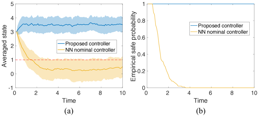
Figure 5: Results in the switching control setting with NN nominal controllers. (a) the average system state over 100 trajectories with its standard deviation. Red dotted line indicates the boundary of the safe set. (b) the empirical safe probability.

VIII Experiments for Reinforcement Learning

In this section, we show experiment results of the proposed safety certificate with reinforcement learning.

We consider system (2) with $f(X_{t})\equiv 0$, $g(X_{t})\equiv 1$, $\sigma(X_{t})\equiv 0.4$. We set $\mathcal{X}=\{0,1,2,\cdots 10\}$ and $\mathcal{U}=\{-1,0,1\}$. The discretized system dynamics with $\Delta t=1$ becomes

$$X_{t+1}=X_{t}+U_{t}+W_{t},$$ (109)

where $X\in\mathcal{X}$ is the state, $U\in\mathcal{U}$ is the control, and $W\in\mathcal{U}$ is the disturbance. The softmax policy $\pi$ is parameterized by $\theta\in\mathbb{R}$ as

$$\pi_{\theta}(U\mid X)\propto\exp(\theta XU).$$ (110)

The reward function $r(x,u):\mathbb{R}^{2}\rightarrow\mathbb{R}$ is set to be

$$r(X,U)=(X-5)/10.$$ (111)

This reward function will encourage visitation of larger $X$. Throughout this section we consider the long-term avoidance safety specification (type 2), where the safety filter $F$ can be acquired through running the proposed method over the following safest-possible nominal policy $\bar{\pi}$, i.e.,

$$\bar{\pi}=\operatorname*{arg\,max}_{\pi}\;\mathbb{P}\left(X_{t}\in{\mathcal{C}}(L_{t}),\forall t\in\{1,\cdots,H\}\right)$$ (112)

where the probability is evaluated assuming $U_{t}\sim\pi(x_{t}),\forall t\in\{1,\cdots,H-1\}$.

VIII-A Policy Gradient

We consider a finite horizon problem with horizon length $H=10$ and initial state $x_{0}=0$. We first run policy gradient without safety filter for 1000 iterations, with 10 episodes per iteration. The policy is updated by

$$\theta_{i+1}=\theta_{i}+\eta_{i}\nabla_{\theta}V^{\pi_{\theta_{i}}}(x_{0}),$$ (113)

where $\eta_{i}$ is the learning rate and is set to be $\eta_{i}=\frac{1}{\sqrt{i}}$ with $i$ being the iteration. We run policy gradient for 1500 iterations with 10 episodes per iteration. The results are shown in Fig 6 in blue lines. We can see that the average reward keeps increasing during training. The learned policy will drive the system’s state to its maximum value to gain better rewards.

We then apply the proposed safety filter to the system. We consider the safe set to be $\mathcal{C}=\{x\in\mathbb{R}:x-5>0\}$, i.e., we want to limit the state transition to any $x>5$ for safety concerns. As a result, we define the following safety filter which corresponds to the probabilistic safety certificate to the safest nominal policy $\bar{\pi}$:

$$G(X,U)=\begin{cases}-1,\quad&X>5\\ U,\quad&\text{otherwise}\end{cases}$$ (114)

Here the safety filter outputs action ‘$-1$’ when $X>5$, otherwise outputs the nominal action $U$. This safety filter (88) can be acquired by running the proposed safe control strategy with $\bar{\pi}$ being the nominal controller. We conduct modified policy gradient described in (92) and the results are shown in Fig. 6 in orange lines. We can see that the learned policy will maximize the return, but will limit the state to safe regions thanks to the safety filter.

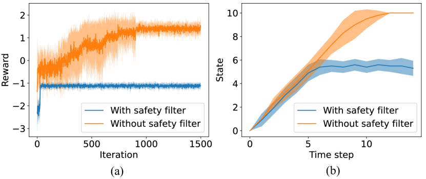
Figure 6: Policy gradient with and without the proposed safety filter. (a) the averaged rewards for 1500 iterations. (b) sample state trajectories with the learned policy.

VIII-B Q-learning

We consider the infinite time horizon problem so that Q function only depends on state and action. We set the discount function to be $\gamma=0.9$ so that the effective horizon is $10$. We set the initial state as $X_{0}=0$. Fig. 7 shows the change of Q function with and without the safety filter. We can see that the Q function will converge in 1500 iterations, and taking action $u=1$ will give the highest Q function value as expected. With the safety filter, the Q function converges to lower values, as the safety filter will limit the visitation of those high-rewarding but unsafe regions in the state space. If we consider greedy policy based on the learned Q function (take action that gives maximized Q function, i.e., $\pi^{Q}(x,u)=\arg\max_{u}Q(x,u)$), we should expect similar control behaviours as policy gradient with and without the safety filter.

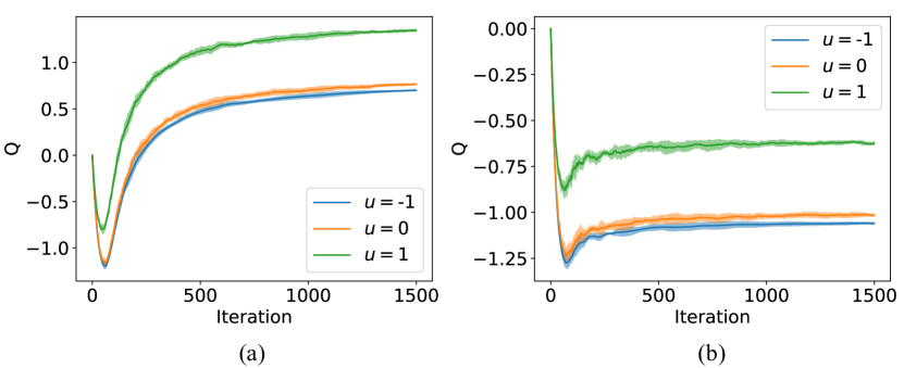
Figure 7: Change of Q function at initial state $x_{0}=0$ (a) without with the safety filter; (b) with the safety filter.

IX Conclusion

This paper focuses on the problem of ensuring long-term safety with high probability in stochastic systems. The major challenge of this problem is the stringent tradeoffs between longer-term safety vs. computational burdens. To mitigate the tradeoffs, we explore how to impose forward invariance on a probability space. Even when set invariance on the state space is satisfied with high probability, long-term safety may not be guaranteed due to the accumulation of uncertainty and risk over time. In contrast, imposing probabilistic invariance on long-term probability allows myopic conditions/controllers to assure long-term design specifications. We then integrate this technique into both control and learning methods. The advantages of the proposed control and learning methods are demonstrated using numerical examples. While beyond the scope of this paper, probabilistic invariance generalizes to settings with unknown dynamics [24], multi-agent coordination [59], and latent risks with unobservable state [60]. The future direction of this research is to explore the probabilistic invariance technique for other control problems currently solved using a set-invariance-based approach, such as constrained optimal control, stability analysis, and robust control [1]. Given the similarity between set invariance and probabilistic invariance, we expect that probabilistic invariance techniques could provide new insights into these problems.

Zhuoyuan Wang received his B.E. degree in Automation from Tsinghua University, Beijing, China, in 2020 and is currently pursuing a Ph.D. degree in Electrical and Computer Engineering at Carnegie Mellon University, Pittsburgh, PA, USA. His research interests include safety-critical control for stochastic systems, physics-informed learning, safe reinforcement learning and application to robotic systems. He is a recipient of the Michel and Kathy Doreau Graduate Fellowship at Carnegie Mellon University.

Haoming Jing received his B.S. degree in Electrical Engineering from University of California, Santa Barbara, Santa Barbara, CA, USA in 2020 and is currently pursuing a Ph.D. degree in Electrical and Computer Engineering at Carnegie Mellon University, Pittsburgh, PA, USA. His research interests include safety-critical control for multi-agent stochastic systems, safety for autonomous driving systems, and safe human-machine interactions.

Christian Kurniawan received a B.Sc. degree in Mathematics from Brigham Young University, Hawaii campus in 2014 and an M.S. degree in Mechanical Engineering with an emphasis on computational grain boundary from Brigham Young University’s main campus in 2018. His current research interest includes applications of optimization techniques and inverse problem theory in various computational engineering problems and autonomous systems.

Albert Chern is an Assistant Professor in Computer Science and Engineering at University of California San Diego, La Jolla, CA, USA, since 2020. He received his Ph.D. in Applied and Computational Mathematics at California Institute of Technology, Pasadena, CA, USA, in 2017, and was a Postdoctoral Researcher in Mathematics at Technische Universität Berlin, Berlin, Germany, from 2017 to 2020. Chern’s research interest lies in applications of differential geometry to computational math, fluid dynamics, computer graphics, and the interplay between stochastic processes and differential equations. Chern was a recipient of the NSF CAREER Award in 2023.

Yorie Nakahira is an Assistant Professor in the Department of Electrical and Computer Engineering at Carnegie Mellon University. She received B.E. in Control and Systems Engineering from Tokyo Institute of Technology in 2012 and Ph.D. in Control and Dynamical Systems from California Institute of Technology in 2019. Her research interests include the fundamental theory of optimization, control, and learning and its application to neuroscience, cell biology, smart grid, cloud computing, finance, autonomous robots.

References

- [1] F. Blanchini, “Set invariance in control,” Automatica, vol. 35, no. 11, pp. 1747–1767, 1999.
- [2] H. Khalil, Nonlinear Systems. Pearson Education, Prentice Hall, 2002.
- [3] A. D. Ames, S. Coogan, M. Egerstedt, G. Notomista, K. Sreenath, and P. Tabuada, “Control barrier functions: Theory and applications,” in 2019 18th European Control Conference (ECC), pp. 3420–3431, IEEE, 2019.
- [4] M. Nagumo, “Über die lage der integralkurven gewöhnlicher differentialgleichungen,” Proceedings of the Physico-Mathematical Society of Japan. 3rd Series, vol. 24, pp. 551–559, 1942.
- [5] J.-M. Bony, “Principe du maximum, inégalité de harnack et unicité du probleme de cauchy pour les opérateurs elliptiques dégénérés,” in Annales de l’institut Fourier, vol. 19, pp. 277–304, 1969.
- [6] H. Brezis, “On a characterization of flow-invariant sets,” Communications on Pure and Applied Mathematics, vol. 23, no. 2, pp. 261–263, 1970.
- [7] A. Clark, “Control barrier functions for stochastic systems,” Automatica, vol. 130, p. 109688, 2021.
- [8] W. Luo, W. Sun, and A. Kapoor, “Multi-robot collision avoidance under uncertainty with probabilistic safety barrier certificates,” arXiv preprint arXiv:1912.09957, 2019.
- [9] Y. Lyu, W. Luo, and J. M. Dolan, “Probabilistic safety-assured adaptive merging control for autonomous vehicles,” in 2021 IEEE International Conference on Robotics and Automation (ICRA), pp. 10764–10770, 2021.
- [10] A. Abate, M. Prandini, J. Lygeros, and S. Sastry, “Probabilistic reachability and safety for controlled discrete time stochastic hybrid systems,” Automatica, vol. 44, no. 11, pp. 2724–2734, 2008.
- [11] M. P. Chapman, J. Lacotte, A. Tamar, D. Lee, K. M. Smith, V. Cheng, J. F. Fisac, S. Jha, M. Pavone, and C. J. Tomlin, “A risk-sensitive finite-time reachability approach for safety of stochastic dynamic systems,” in 2019 American Control Conference (ACC), pp. 2958–2963, IEEE, 2019.
- [12] N. Kariotoglou, S. Summers, T. Summers, M. Kamgarpour, and J. Lygeros, “Approximate dynamic programming for stochastic reachability,” in 2013 European Control Conference (ECC), pp. 584–589, IEEE, 2013.
- [13] A. Abate, S. Amin, M. Prandini, J. Lygeros, and S. Sastry, “Probabilistic reachability and safe sets computation for discrete time stochastic hybrid systems,” in Proceedings of the 45th IEEE Conference on Decision and Control, pp. 258–263, IEEE, 2006.
- [14] W. Liao, T. Liang, X. Wei, and Q. Yin, “Probabilistic reach-avoid problems in nondeterministic systems with time-varying targets and obstacles,” Applied Mathematics and Computation, vol. 425, p. 127054, 2022.
- [15] M. Vasileva, F. Shmarov, and P. Zuliani, “Probabilistic reachability for uncertain stochastic hybrid systems via gaussian processes,” in 2020 18th ACM-IEEE International Conference on Formal Methods and Models for System Design (MEMOCODE), pp. 1–11, IEEE, 2020.
- [16] S. Bansal, M. Chen, S. Herbert, and C. J. Tomlin, “Hamilton-jacobi reachability: A brief overview and recent advances,” in 2017 IEEE 56th Annual Conference on Decision and Control (CDC), pp. 2242–2253, IEEE, 2017.
- [17] J. J. Choi, D. Lee, K. Sreenath, C. J. Tomlin, and S. L. Herbert, “Robust control barrier-value functions for safety-critical control,” in 2021 60th IEEE Conference on Decision and Control (CDC), pp. 6814–6821, IEEE, 2021.
- [18] A. Clark, “Control barrier functions for complete and incomplete information stochastic systems,” in 2019 American Control Conference (ACC), pp. 2928–2935, IEEE, 2019.
- [19] S. Prajna, A. Jadbabaie, and G. J. Pappas, “A framework for worst-case and stochastic safety verification using barrier certificates,” IEEE Transactions on Automatic Control, vol. 52, no. 8, pp. 1415–1428, 2007.
- [20] S. Yaghoubi, K. Majd, G. Fainekos, T. Yamaguchi, D. Prokhorov, and B. Hoxha, “Risk-bounded control using stochastic barrier functions,” IEEE Control Systems Letters, 2020.
- [21] C. Santoyo, M. Dutreix, and S. Coogan, “A barrier function approach to finite-time stochastic system verification and control,” Automatica, p. 109439, 2021.
- [22] C. Huang, X. Chen, W. Lin, Z. Yang, and X. Li, “Probabilistic safety verification of stochastic hybrid systems using barrier certificates,” ACM Transactions on Embedded Computing Systems (TECS), vol. 16, no. 5s, pp. 1–19, 2017.
- [23] M. Anand, P. Jagtapt, and M. Zamani, “Verification of switched stochastic systems via barrier certificates,” in 2019 IEEE 58th Conference on Decision and Control (CDC), pp. 4373–4378, IEEE, 2019.
- [24] S. Gangadhar, Z. Wang, H. Jing, and Y. Nakahira, “Adaptive safe control for driving in uncertain environments,” in 2022 IEEE Intelligent Vehicles Symposium (IV), pp. 1662–1668, IEEE, 2022.
- [25] M. Farina, L. Giulioni, and R. Scattolini, “Stochastic linear Model Predictive Control with chance constraints – A review,” Journal of Process Control, vol. 44, pp. 53–67, aug 2016.
- [26] L. Hewing, K. P. Wabersich, M. Menner, and M. N. Zeilinger, “Learning-Based Model Predictive Control: Toward Safe Learning in Control,” Annual Review of Control, Robotics, and Autonomous Systems, vol. 3, pp. 269–296, may 2020.
- [27] S. Gu, L. Yang, Y. Du, G. Chen, F. Walter, J. Wang, Y. Yang, and A. Knoll, “A review of safe reinforcement learning: Methods, theory and applications,” arXiv preprint arXiv:2205.10330, 2022.
- [28] J. Garcıa and F. Fernández, “A comprehensive survey on safe reinforcement learning,” Journal of Machine Learning Research, vol. 16, no. 1, pp. 1437–1480, 2015.
- [29] T. Xu, Y. Liang, and G. Lan, “Crpo: A new approach for safe reinforcement learning with convergence guarantee,” in International Conference on Machine Learning, pp. 11480–11491, PMLR, 2021.
- [30] Y. Chen, J. Dong, and Z. Wang, “A primal-dual approach to constrained markov decision processes,” arXiv preprint arXiv:2101.10895, 2021.
- [31] Y. Liu, A. Halev, and X. Liu, “Policy learning with constraints in model-free reinforcement learning: A survey,” in The 30th International Joint Conference on Artificial Intelligence (IJCAI), 2021.
- [32] A. Wachi and Y. Sui, “Safe reinforcement learning in constrained markov decision processes,” in International Conference on Machine Learning, pp. 9797–9806, PMLR, 2020.
- [33] Y. Chow, O. Nachum, E. Duenez-Guzman, and M. Ghavamzadeh, “A lyapunov-based approach to safe reinforcement learning,” Advances in neural information processing systems, vol. 31, 2018.
- [34] C. Qin, J. Wang, H. Zhu, J. Zhang, S. Hu, and D. Zhang, “Neural network-based safe optimal robust control for affine nonlinear systems with unmatched disturbances,” Neurocomputing, vol. 506, pp. 228–239, 2022.
- [35] T. Wei and C. Liu, “Safe control with neural network dynamic models,” in Learning for Dynamics and Control Conference, pp. 739–750, PMLR, 2022.
- [36] H. Zhao, X. Zeng, T. Chen, Z. Liu, and J. Woodcock, “Learning safe neural network controllers with barrier certificates,” Formal Aspects of Computing, vol. 33, pp. 437–455, 2021.
- [37] G. N. Tasse, T. Love, M. Nemecek, S. James, and B. Rosman, “Rosarl: Reward-only safe reinforcement learning,” arXiv preprint arXiv:2306.00035, 2023.
- [38] S. Amani, C. Thrampoulidis, and L. Yang, “Safe reinforcement learning with linear function approximation,” in International Conference on Machine Learning, pp. 243–253, PMLR, 2021.
- [39] P. L. Donti, M. Roderick, M. Fazlyab, and J. Z. Kolter, “Enforcing robust control guarantees within neural network policies,” arXiv preprint arXiv:2011.08105, 2020.
- [40] K. Srinivasan, B. Eysenbach, S. Ha, J. Tan, and C. Finn, “Learning to be safe: Deep rl with a safety critic,” arXiv preprint arXiv:2010.14603, 2020.
- [41] M. Alshiekh, R. Bloem, R. Ehlers, B. Könighofer, S. Niekum, and U. Topcu, “Safe reinforcement learning via shielding,” in Proceedings of the AAAI Conference on Artificial Intelligence, vol. 32, 2018.
- [42] B. Øksendal, Stochastic Differential Equations: An Introduction with Applications. Universitext, Berlin Heidelberg: Springer-Verlag, sixth ed., 2003.
- [43] A. N. Borodin, Stochastic processes. Springer, 2017.
- [44] A. Chern, X. Wang, A. Iyer, and Y. Nakahira, “Safe control in the presence of stochastic uncertainties,” in 2021 60th IEEE Conference on Decision and Control (CDC), pp. 6640–6645, IEEE, 2021.
- [45] J. L. W. V. Jensen, “Sur les fonctions convexes et les inégalités entre les valeurs moyennes,” Acta Mathematica, vol. 30, pp. 175–193, 1906.
- [46] Q. Zhang, A. Taghvaei, and Y. Chen, “An optimal control approach to particle filtering,” Automatica, vol. 151, p. 110894, 2023.
- [47] S. Thijssen and H. Kappen, “Path integral control and state-dependent feedback,” Physical Review E, vol. 91, no. 3, p. 032104, 2015.
- [48] B. Oksendal, Stochastic differential equations: an introduction with applications. Springer Science & Business Media, 2013.
- [49] Z. Wang and Y. Nakahira, “A generalizable physics-informed learning framework for risk probability estimation,” in Learning for Dynamics and Control Conference, pp. 358–370, PMLR, 2023.
- [50] Z. Wang, R. Keller, X. Deng, K. Hoshino, T. Tanaka, and Y. Nakahira, “Physics-informed representation and learning: Control and risk quantification,” in Proceedings of the AAAI Conference on Artificial Intelligence, vol. 38, pp. 21699–21707, 2024.
- [51] H. Hoshino and Y. Nakahira, “A physics-informed reinforcement learning framework for risk probability estimation,” in American Control Conference, 2024.
- [52] E. Marcus, R. Sheombarsing, J.-J. Sonke, and J. Teuwen, “Constrained empirical risk minimization: Theory and practice,” arXiv preprint arXiv:2302.04729, 2023.
- [53] C. E. Garcia, D. M. Prett, and M. Morari, “Model predictive control: Theory and practice—a survey,” Automatica, vol. 25, no. 3, pp. 335–348, 1989.
- [54] D. Q. Mayne, J. B. Rawlings, C. V. Rao, and P. O. Scokaert, “Constrained model predictive control: Stability and optimality,” Automatica, vol. 36, no. 6, pp. 789–814, 2000.
- [55] R. S. Sutton and A. G. Barto, Reinforcement learning: An introduction. MIT press, 2018.
- [56] C. J. Watkins and P. Dayan, “Q-learning,” Machine learning, vol. 8, pp. 279–292, 1992.
- [57] C. Gaskett, D. Wettergreen, and A. Zelinsky, “Q-learning in continuous state and action spaces,” in Australasian joint conference on artificial intelligence, pp. 417–428, Springer, 1999.
- [58] M. Ahmadi, X. Xiong, and A. D. Ames, “Risk-sensitive path planning via cvar barrier functions: Application to bipedal locomotion,” arXiv preprint arXiv:2011.01578, 2020.
- [59] H. Jing and Y. Nakahira, “Probabilistic safety certificate for multi-agent systems,” in 2022 61th IEEE Conference on Decision and Control (CDC), IEEE, 2022.
- [60] S. Gangadhar, Z. Wang, K. Poku, N. Yamada, K. Honda, Y. Nakahira, H. Okuda, and T. Suzuki, “An occlusion- and interaction-aware safe control strategy for autonomous vehicles,” in 2023 22nd IFAC World Congress, 2023.