Worldwide wildfire spreading and its severity described by the SIR model

Abstract:

One-Sentence Summary:

Introduction

Results

Fire dynamics modeling

Continent	Number of fire events
Africa	23479770
South America	6190501
Asia	6090517
North America	2324829
Europe	2324584
Oceania	1192404
Seven Seas	1411
Global	41789913

Table 1: Number of fire events from year 2002 to 2023 at continent level.

Continent	Burned Area (million km2)
Africa	96.34
South America	26.41
Asia	20.07
Europe	10.78
Oceania	9.84
North America	9.26
Seven Seas	3.00
Global	173.32

Table 2: Burned Area in million square kilometers from year 2002 to 2023 at continent level.

Top-10 Countries	Number of fire events
Democratic Republic of the Congo	4748743
Brazil	3516396
Angola	2934788
Zambia	2090508
Central African Republic	1554983
Russia	1545821
Mozambique	1517531
People’s Republic of China	1241056
South Sudan	1200230
Australia	1073981

Table 3: Top 10 countries with the total number of fire events.

Top-10 Countries	Burned Area (million km2)
Democratic Republic of the Congo	18.52
Brazil	15.43
Angola	14.38
Australia	9.51
Zambia	8.43
Russia	8.33
South Sudan	7.06
Central African Republic	6.45
Mozambique	5.83
United State of America	3.80

Table 4: Top 10 countries with Burned Area.

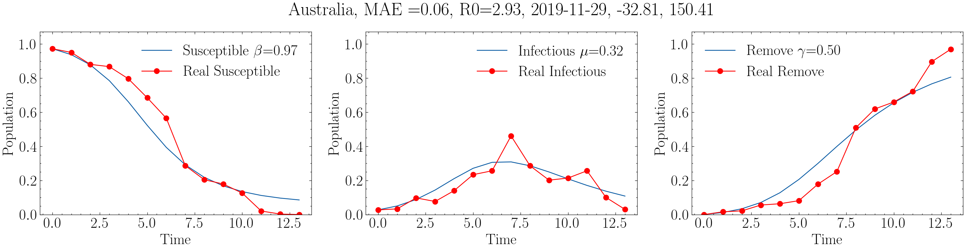
(a) 2019-2020 Australian Bushfire Season

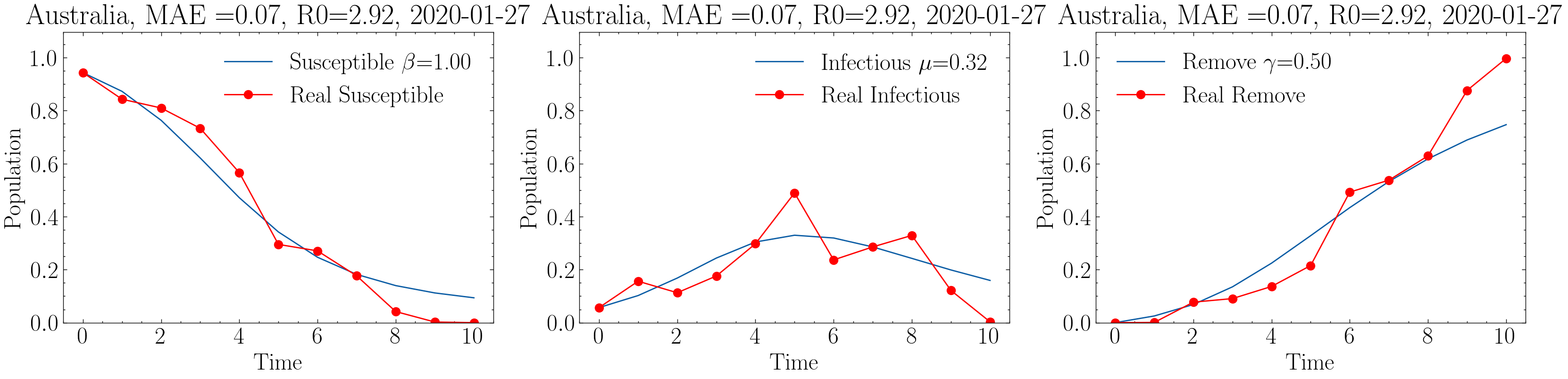
(b) 2019-2020 Australian Bushfire Season

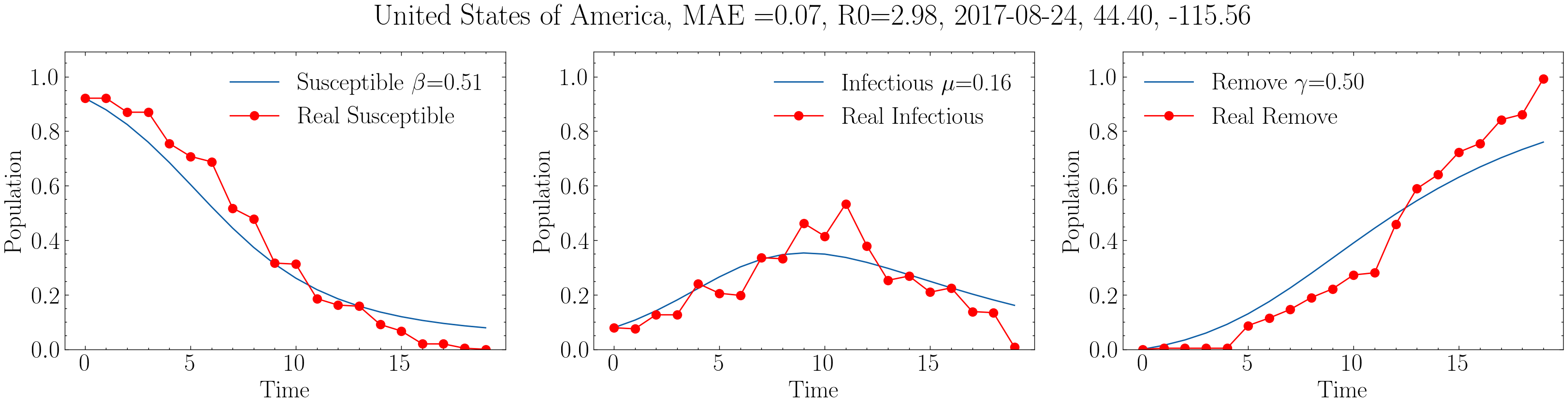
(c) Bearskin Fire in Idaho

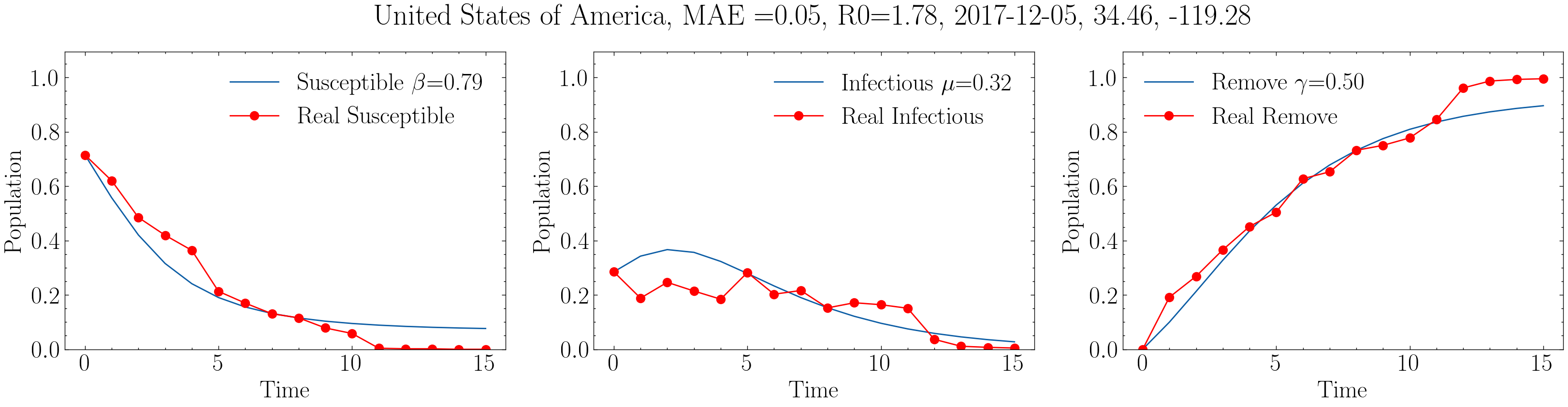
(d) Southern California wildfires

Figure 1: SIR dynamics for a fire event in Australia and the United State of America, respectively.

We estimate that from 2002 to 2020, there are in total 36527974 recorded wildfires around the world, near two million fire events per year. At the continent level, we summarized the total number of recorded wildfires and the Burned Area (BA) for each continent in Table 1 and 2, where Africa (20392837, 84.20 million km²) was found to to have highest contribution to the number of wildfires, followed by South America (5435623, 23.24 million km²), Asia (5335222, 17.87 million km²) and Europe (2151347, 9.83 million km²). At the country level, as shown in Table 3, Democratic Republic of the Congo shares the largest number of wildfires in the past two decades, followed by Brazil, Angola and Zambia. For the country ranking of BA (Table 4), Democratic Republic of the Congo is also the top country, followed by Brazil, Angola and Australia.

Among the fire events, every year worldwide some extraordinary wildfires occur, overwhelming suppression capabilities, causing substantial damages, and often resulting in fatalities  (?). For example, extreme, long-duration wildfires in the western USA in 2017  (?), and in eastern Australia in 2019-2020  (?) had attracted social attention. Here, we take the above-mentioned fire events as examples to demonstrate the dynamics of fire events and provide the metric of the fire spread (Fig. 1). The dynamics of fire events can be well-modeled by the susceptible-infected-recovered (SIR) model, details of which will be shown in Data and methods. The observed number of spatio-temporal fire grids for each compartment (compartment $S$: left subplot; compartment $I$: middle subplot; compartment $R$: right subplot) can be well described with the SIR model, with the Mean Absolute Errors (MAEs) are (a) 0.06; (b) 0.07; (c) 0.07; (d) 0.05. The basic reproductive number, $R_{0}$ , which is calculated per event, represents the average number of secondary fire grids ignited by a primary fire event, serving as a key metric of its potential to spread rapidly. For extreme fire events in Fig. 1, $R_{0}$ are (a) 2.93 (b) 2.92 (c) 2.98 and (d)1.78. Fitting empirical data with SIR model, a set of $R_{0}$ for all events of interest can be obtained.

Global distribution of averaged $R_{0}$ during 2002-2023

(We found a more clustered distribution of $R_{0}$ . ) We found that there exists obvious heterogeneity in the global distribution of averaged $R_{0}$ per event during 2002-2020, as shown in Fig. 3. Middle East, North Africa, Northeast India, Kazakhstan, and Central Russia share relatively high value of $R_{0}$ (greater than 5). At the continent level, as shown in Table 5, Asia takes the lead with an averaged $R_{0}$ of 5.90, followed by Africa (4.68), Europe (4.54) and North America (4.11). At the country level, Eritrea (9.52), The Bahamas (8.11), Netherlands (7.96) are the ranked Top-3 $R_{0}$ countries as shown in the ranking plot Fig. 2 and Table 6, followed by Kosovo (7.55) and Libya (7.41).

Continent	$R_{0}$	MAE
Asia	5.90	0.09
Africa	4.68	0.10
Europe	4.54	0.09
North America	4.11	0.09
South America	4.00	0.09
Oceania	2.87	0.11
Seven Seas	2.78	0.12
Global	4.79	0.10

Table 5:

Top-10 Countries	$R_{0}$	MAE
Eritrea	9.52	0.06
The Bahamas	8.11	0.05
Netherlands	7.96	0.12
Kosovo	7.55	0.20
Libya	7.41	0.09
Latvia	7.34	0.09
Greenland	7.33	0.08
Estonia	7.15	0.10
Syria	6.54	0.10
Spain	6.50	0.11

Table 6:

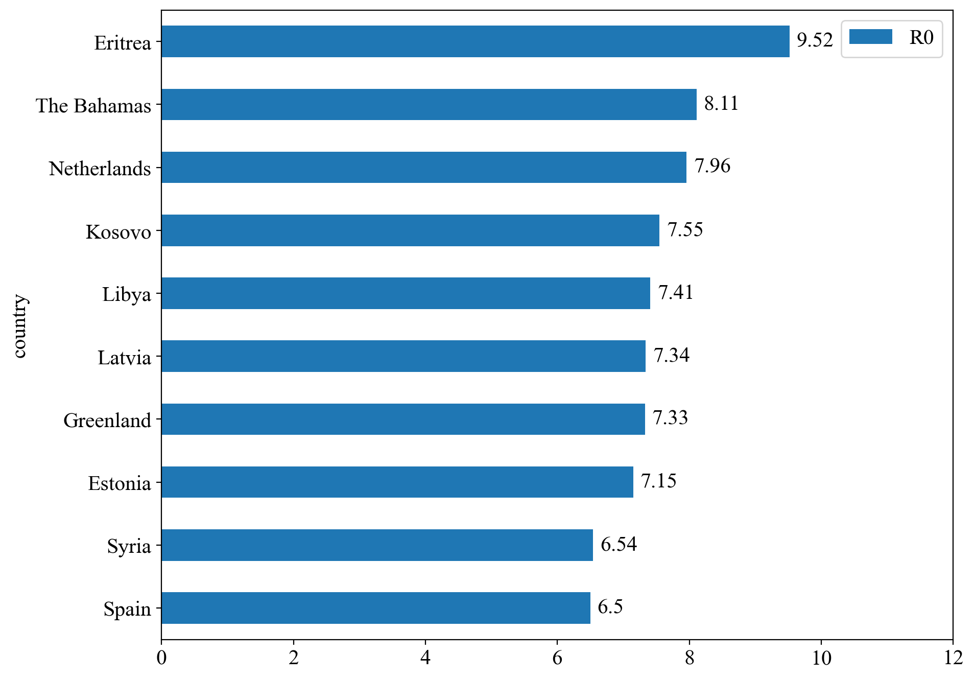
Figure 2: Top 10 countries for $R_{0}$ .

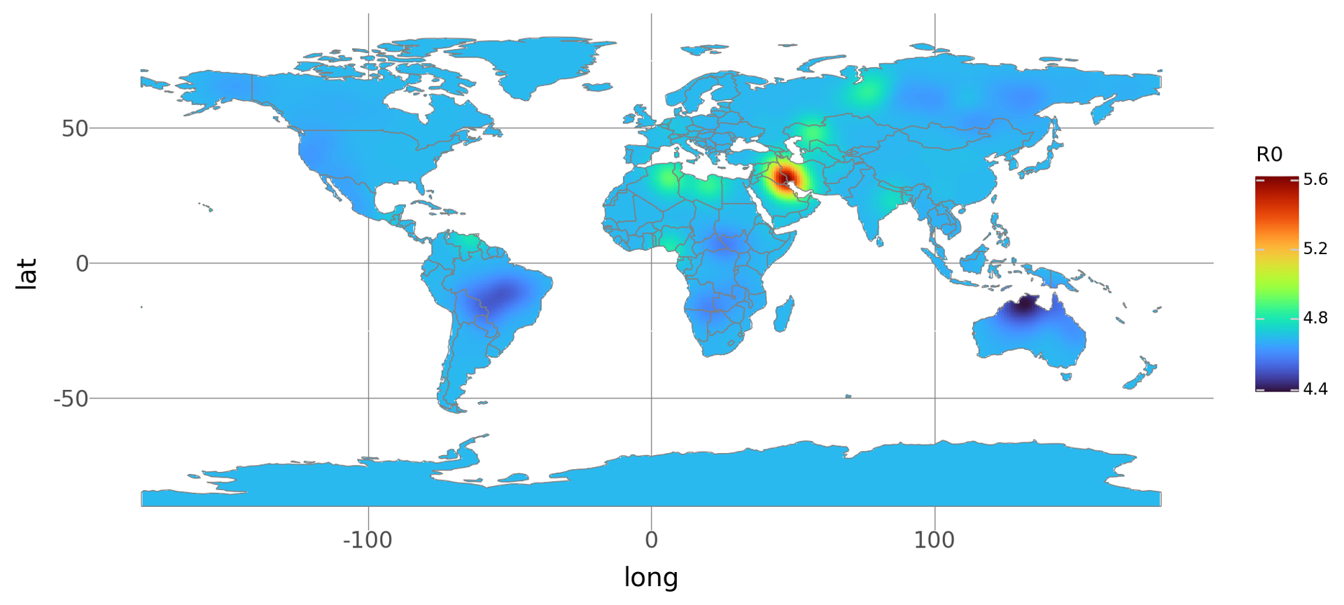
Figure 3: Global distribution of averaged $R_{0}$ over two decades.

Figure 4: Correlation matrix between $R_{0}$ , duration, Burned Area (BA) and maximum Fire Radiative power (max FRP).

Historical evolution of global $R_{0}$ during 2002-2023

The past twenty years have seen the dramatic evolution of global pattern of $R_{0}$. Time series of global $R_{0}$ in Fig. 5g presents an annual trend of global $R_{0}$ from 2002 to 2020 for the fire events lasting more than 9 days. Quantitative findings indicate a substantial increase of 8% in the global $R_{0}$ between 2002 ($R_{0}$ = 4.47) and 2020 ($R_{0}$ = 4.82). The evolution of global $R_{0}$ fluctuated substantially but we can still observe a slightly increase by 0.02 annually. With an areal aggregation by continents, from Fig. 5a-5f and Table 7, we found a small growth trend of $R_{0}$ for most continents over two decades, except for Europe ($R_{0}$ decreases by 0.02 per year). To demonstrate a general variation of the fire amount and severity for an area per decade, we also summed up $R_{0}$ of all event in each decade and defined a variation ratio, $\rho=(\frac{\sum_{i}R_{0}^{i}(2013-2023)}{\sum_{i}R_{0}^{i}(2002-2012)}-1)/100\%$, where $i$ is the index of fire events. Globally, $\rho$ is estimated to be 41%, means that the sum of $R_{0}$ of all events in 2013-2023 has increased by 41%, compared with that in 2002-2012. Of this total growth, Oceania, North America, and Asia have leading contribution, with the variation ratio per decade are 53%, 52%, and 51%, respectively.

The global spatial distributions of $R_{0}$ in Fig. 6a and 6bshows different patterns between the two decades (2002–20012 and 2013–2023), In Fig. 6c, from 2002 to 2023, $R_{0}$ showed statistically significant increasing trends in Middle East, Western North America, Western Australia, Africa, and South America, whereas notable decreasing trends were found in Eastern North America and Eastern Russia.

Fig. 7 shows detailed analyses that are applied to some countries of hotspot, e.g., Australia, The United State of America, and Brazil, where extreme, long-duration wildfires happened.

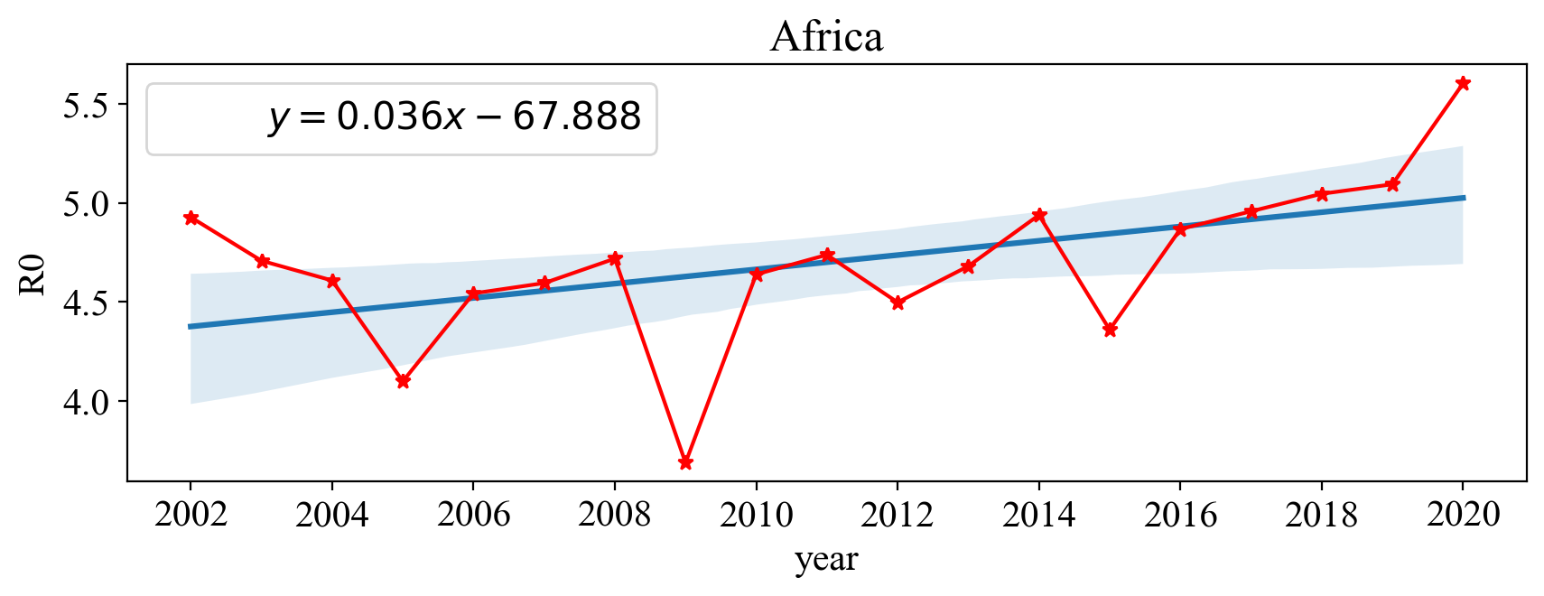
(a) Africa

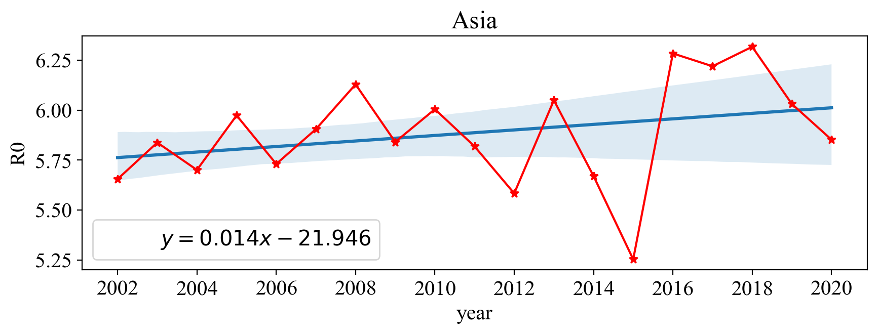
(b) Asia

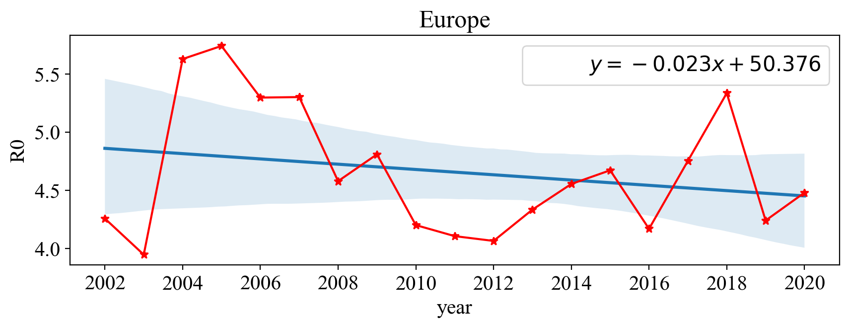
(c) Europe

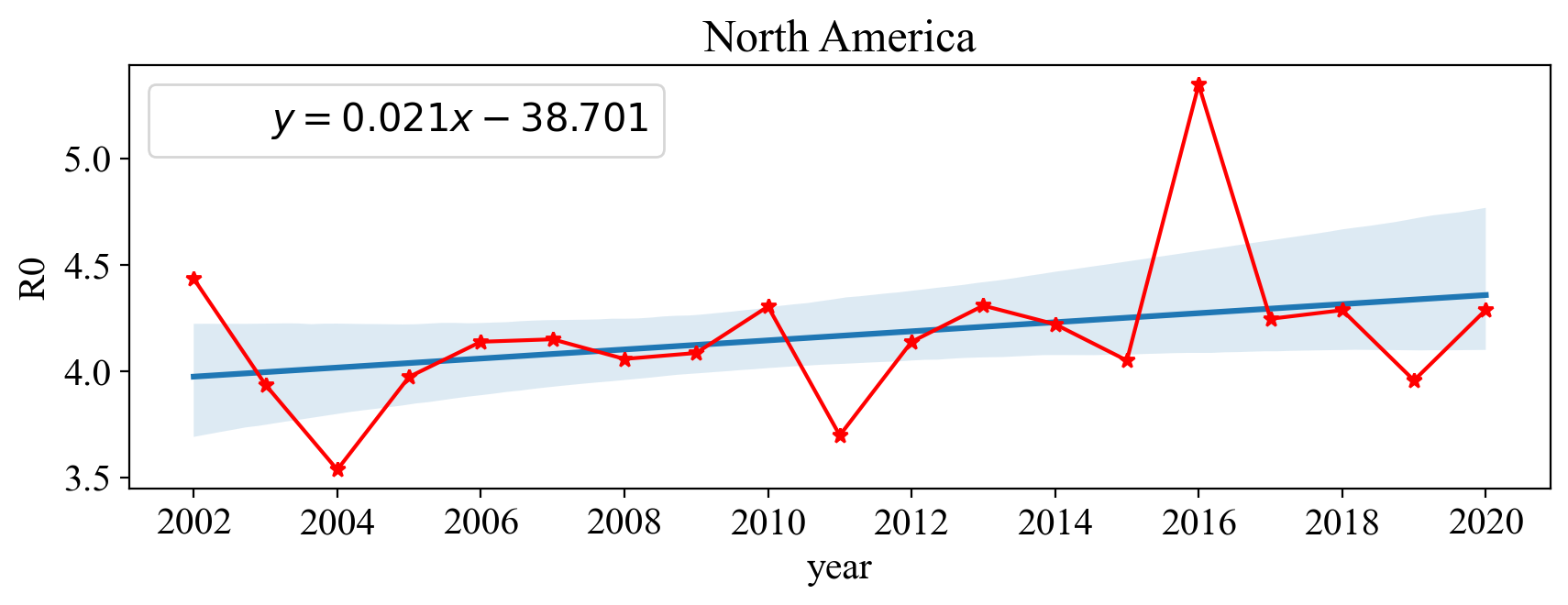
(d) North America

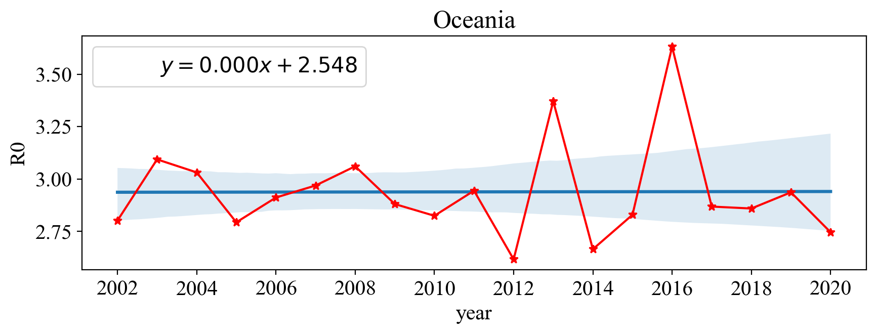
(e) Oceania

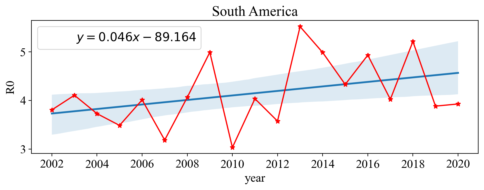
(f) South America

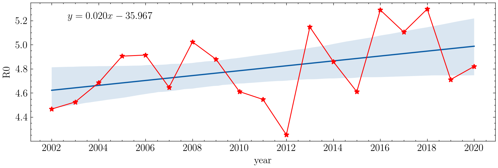
(g) Global

Figure 5: Annual trend of global $R_{0}$ for the fire events lasting more than 9 days.

Continent	$R_{0}$ Slope	$\rho$ (%)
Africa	0.04	12
Asia	0.01	51
Europe	-0.02	29
North America	0.02	52
Oceania	0.00	53
South America	0.05	42
Global	0.02	41

Table 7: $\rho=(\frac{\sum_{i}R_{0}^{i}(2013-2023)}{\sum_{i}R_{0}^{i}(2002-2012)}-1)/100\%$, where i is the index of fire events.

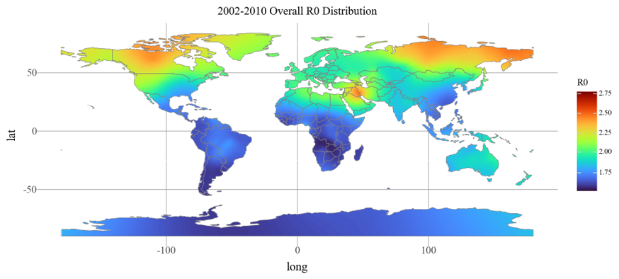
(a)

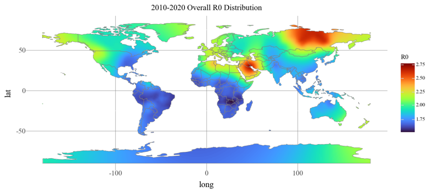
(b)

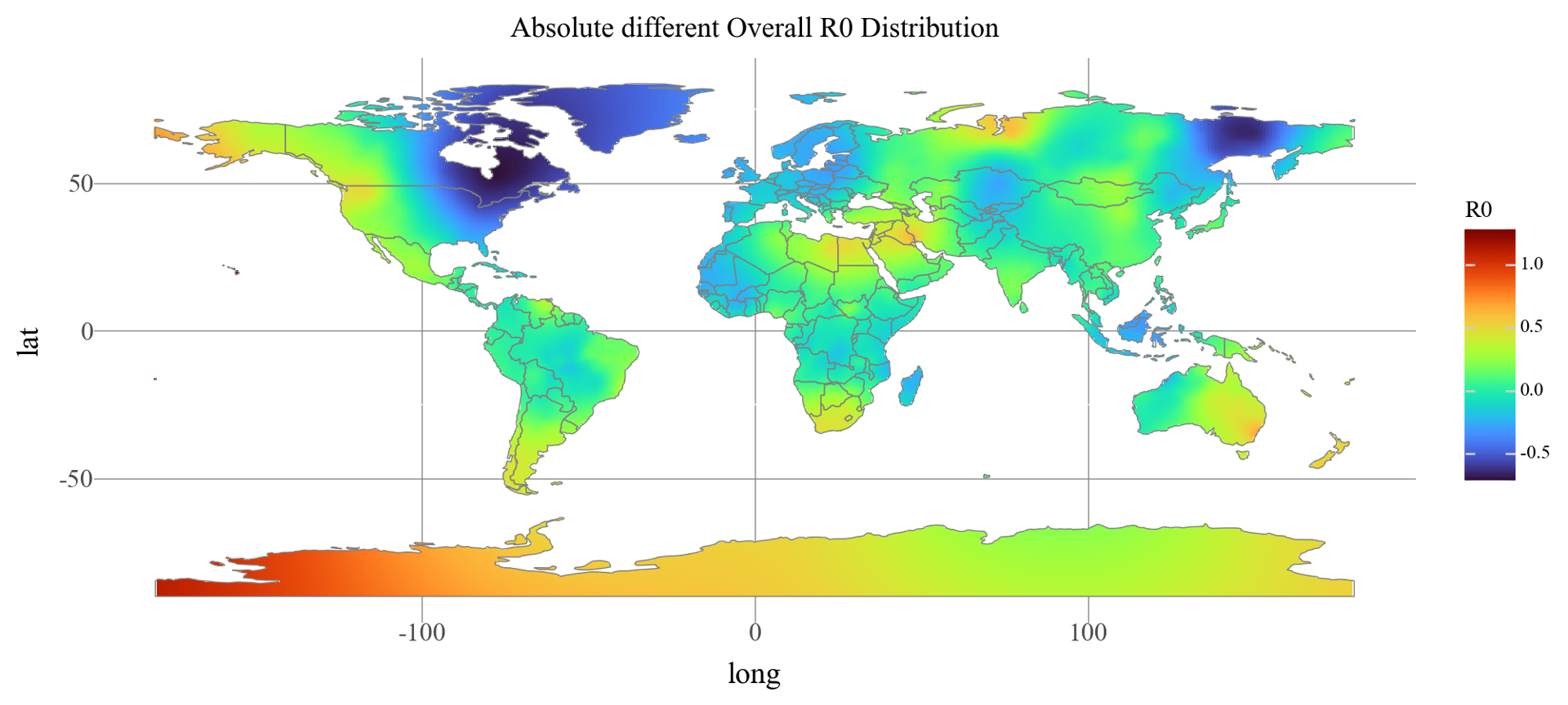
(c)

Figure 6: Global distribution of averaged $R_{0}$ in the first (a) and second (b) decades of 2002-2020, and the trend during this period (changes per decade).

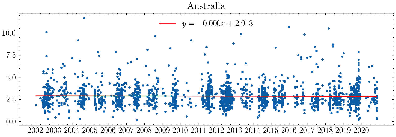
(a)

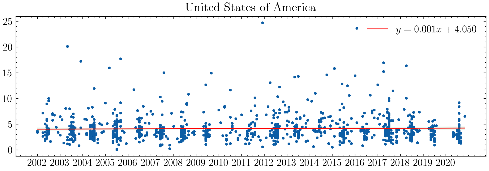
(b)

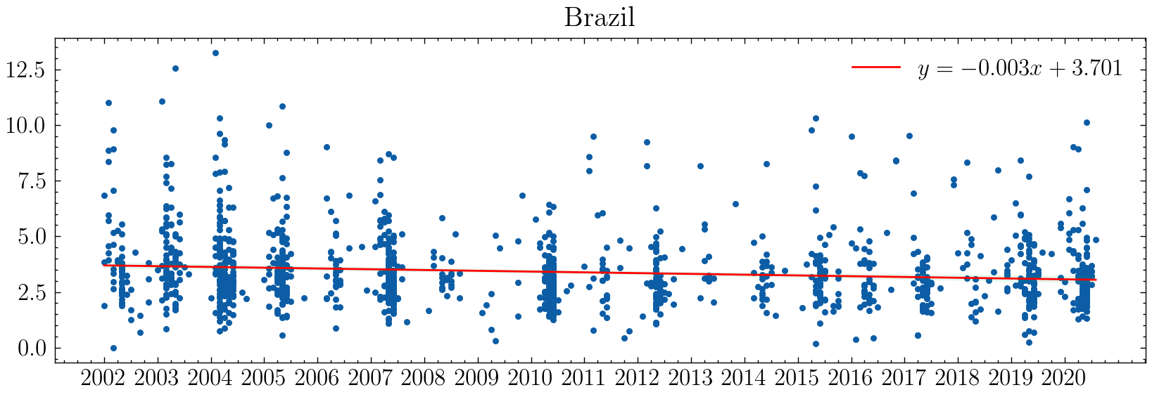
(c)

Figure 7: R0 distribution from year 2002 to 2020 in Australia, The United State of America and Brazil, respectively. Fire events are filtered

Discussion

Data and methods

Wildfire data

We use the novel FireTracks (FT) Scientific Dataset  (?) of individual fires. The FT algorithm employs network theory and the individual fires approach to aggregate fire events into spatio-temporal fire clusters that are tracked over space and time. Individual fires are the union of nearest neighbours of active fires in the discrete spacetime grid given by the spatial and temporal resolution of the Moderate Resolution Imaging Spectroradiometer (MODIS) 1-km MOD/MYD14A1 Thermal Anomalies and Fire dataset (Giglio and Justice 2015) that feeds the algorithm. Two fire events are considered neighbours if they are in the same 3-dimensional (latitude, longitude, time) Moore neighbourhood with no spatial or temporal gaps (Fig. 1b). The MOD/MYD14A1 fire product offers an indication of fire activity and has been extensively validated (Morisette et al. 2005; Csiszar et al. 2006; Hawbaker et al. 2008; de Klerk 2008). The collection 6 of the data addresses previous limitations such as frequent false alarms caused by small clearings in the Amazon forests (Friedl et al. 2010), which is particularly helpful for our purpose. The data present low levels of commission errors, but omission errors, which decrease as fire size increases, might occur with fires of short duration, small size or low intensity (Schroeder et al. 2008; Hantson et al. 2013). Also, burnings under dense vegetation cover, heavy smoke or clouds may go undetected (Giglio et al. 2016).

The FT dataset registers location, time and land cover of individual fires at daily time step, as well as their estimated size, intensity, duration and rate of spread (see Text S1 for the definition of the fire variables). The smallest identifiable fire size and duration is imposed by the spatio-temporal resolution of the MODIS fire data, 0.86 km2 and one day, respectively. Fires with sizes smaller than one fire-data pixel are attributed a size of 0.86 km2 regardless, which may generate some overestimation of burned area. Fires of a single fire-data pixel size (0.86 km2) are not considered for the calculation of rate of spread—the ratio between size and duration. We select those fires within the BLA over the time period from 2002 to 2020 in six land-cover types: croplands, deciduous forests, grasslands, evergreen forests, savannas and woody savannas (see Text S2 and Fig. S2 for the description and spatial distribution of the different land covers, respectively).

The FT algorithm combines the MODIS fire data with land-cover information from the previous year. We use the UMD classification scheme of the 500-m Land Cover Type MCD12Q1 product from MODIS (Sulla Menashe et al. 2019). The collection 6 of the land-cover data includes new gap-filled spectro-temporal features and refinements of the algorithm, which allows a more accurate classification. However, some limitations are known, e.g. grassland areas might be misclassified as savannas, and agriculture can be underrepresented in tropical regions where agricultural fields are small (Friedl et al. 2010). Since the land-cover data has a spatial resolution twice as high as the active fires data (0.21 vs. 0.86 km2), the FT algorithm associates four values of land cover with every MODIS active fire within a particular individual fire. Fires are assigned a dominant land cover when at least 80% of all the land-cover values within them belong to the same land-cover type. Fires that do not fulfil this criterion are discarded from the analysis. In this way, we ensure that the FT’s fire characteristics estimated for each land-cover type are not a combination of values from different land covers.

We employ the GFA dataset (Andela et al. 2019b), the most extensive study on individual fires covering the BLA so far, to perform a comparison of our estimated fire characteristics. The GFA is derived from the MODIS collection 6 500-m Burned Area MCD64A1 product (Giglio et al. 2018) and spans from 2003 to 2016. The quality of the algorithm, as for the FT’s, highly depends on the inherent limitations of the data that serve as input. Fires of 0.21 km2—the smallest identifiable fire size—are not taken into account when calculating rate of spread. The GFA algorithm tracks the daily progression of individual fires to produce a set of metrics on fire behaviour such as fire size, duration, daily expansion, fire line length, speed and direction of spread. We select from the FT dataset the fires identified in the BLA over the period 2003–2016—the same 14-year time window when data from the GFA is available—and compare fire size, duration and rate of spread—the variables present in both datasets—occurring in croplands, forests, grasslands and savannas (Text S2).

Methods

Wildfire dynamics

To well model the spread and describe the dynamics of each fire event, we use a well-known compartment model called susceptible-infected-recovered (SIR) with susceptible ($S$), Infectious ($I$), and Removed ($R$) compartments. Within the perimeter of an individual fire, there are N spatio-temporal fire grids in total. Susceptible spatio-temporal grids are flammable but have never been burned yet, while they can get ignited through contact with a primary fire event. Burning grids are categorized into Infectious state. Then, fires will get extinguished or go out after a period of time, meaning Infectious s will transition into the Removed state. The removed state represents fires can no longer resurge once gone out.

Thus, analogous to the modeling of infectious disease spread in a population, the dynamics of an individual fire $i$ can be described by SIR model:

$$\frac{dS_{i}(t)}{dt}= -\beta S_{i}(t)I_{i}(t)$$

$$\frac{dI_{i}(t)}{dt}= \beta S_{i}(t)I_{i}(t)-\mu I_{i}(t)$$

$$\frac{dR_{i}(t)}{dt}= \mu I_{i}(t)$$

where $\beta$ represents the transmission rate of an individual fire event, and $\mu$ represents the dissipation rate of the fire. $\beta\in[0,1]$ and $\mu\in[\frac{1}{d},1]$ where $d$ is the duration of a fire event. We introduce a basic reproduction number, $R_{0}=\frac{\beta S(0)}{\mu}$, which represents the average number of secondary infections produced by a single infected individual in a completely susceptible population (i.e. $S(t)=S(0)$). Fitting the empirical data with the SIR model, one can obtain an evaluable criteria, $R_{0}$, according to which the government or managers can appraise the fire risk of jurisdictions.

Learning the relationship between $R_{0}$ and land-cover types

Conventionally, fire regimes (or behaviors) is characterized by a few parameters  (?): fire size, duration, fireline intensity (FLI), Rate of Spread (ROS), spotting, flame length (FL), etc. For example, Ana Cano‑Crespo et al.  (?) analyzed fire regimes in six different land-cover classes. Fires in savannas and evergreen forests were found to burn the largest areas and are the most long lasting. Inspired by their analysis, in this paper, the correlation between $R_{0}$ and different land-cover types is studied. Rather than assuming a specific statistical or functional relationship between $R_{0}$ and land-cover types, we learn it directly from the data. Specifically, we use neural networks and random forests to learn the potentially nonlinear relationship in ways that are highly conditional on the state of other environmental variables.

Supplementary materials

Materials and Methods
Figs S1 to S17
Tables S1 to S14
References (58-69)

Figure 2: Social utility and equity of vaccine distribution strategies that prioritize disadvantaged communities under a single demographic dimension. (a) Changes in social utility and equity, compared to the Homogeneous baseline. The red/blue points respectively represent the strategies prioritizing the most/least disadvantaged communities. The $1^{st}$ to $4^{th}$ quadrant respectively represents: (i) simultaneously improving utility and equity, (ii) improving equity but damaging utility, (iii) improving utility but damaging equity, and (iv) simultaneously damaging utility and equity. (b) Changes in three dimensions of equity, compared to the Homogeneous baseline. Highlighted grids indicate degradation in the corresponding dimension of equity. (c) Social utility under different scenarios of vaccine hesitancy. When vaccine hesitancy in low-income communities is stronger, the benefit on social utility brought by prioritizing disadvantaged communities diminishes. In extreme scenarios, the benefit of prioritizing disadvantaged communities characterized by income is completely erased, making it inferior to the baseline. (d) Joint probability distribution of demographic features, where brighter colors indicate larger probability density. The correlations between (i) the percentage of older adults and the average household income, (ii) the percentage of older adults and the percentage of essential workers, (iii) the average household income and the percentage of essential workers are (i) $+0.14$, (ii) $-0.2$, and (iii) $+0.28$, respectively, displaying the mismatch among disadvantaged communities in different demographic dimensions.

References

- 1. Niels Andela, Douglas C Morton, Louis Giglio, Yang Chen, Guido R Werf, Prasad S Kasibhatla, Rurth S DeFries, GJ Collatz, S Hantson and Silvia Kloster “A human-driven decline in global burned area” In Science 356.6345 American Association for the Advancement of Science, 2017, pp. 1356–1362
- 2. Aurora A Gutierrez, Stijn Hantson, Baird Langenbrunner, Bin Chen, Yufang Jin, Michael L Goulden and James T Randerson “Wildfire response to changing daily temperature extremes in California’s Sierra Nevada” In Science advances 7.47 American Association for the Advancement of Science, 2021, pp. eabe6417
- 3. A Park Williams, John T Abatzoglou, Alexander Gershunov, Janin Guzman-Morales, Daniel A Bishop, Jennifer K Balch and Dennis P Lettenmaier “Observed impacts of anthropogenic climate change on wildfire in California” In Earth’s Future 7.8 Wiley Online Library, 2019, pp. 892–910
- 4. Marco Turco, Juan José Rosa-Cánovas, Joaquín Bedia, Sonia Jerez, Juan Pedro Montávez, Maria Carmen Llasat and Antonello Provenzale “Exacerbated fires in Mediterranean Europe due to anthropogenic warming projected with non-stationary climate-fire models” In Nature communications 9.1 Nature Publishing Group UK London, 2018, pp. 3821
- 5. Bin Chen, Yufang Jin, Erica Scaduto, Max A Moritz, Michael L Goulden and James T Randerson “Climate, fuel, and land use shaped the spatial pattern of wildfire in California’s Sierra Nevada” In Journal of Geophysical Research: Biogeosciences 126.2 Wiley Online Library, 2021, pp. e2020JG005786
- 6. Stephanie E Mueller, Andrea E Thode, Ellis Q Margolis, Larissa L Yocom, Jesse D Young and Jose M Iniguez “Climate relationships with increasing wildfire in the southwestern US from 1984 to 2015” In Forest Ecology and Management 460 Elsevier, 2020, pp. 117861
- 7. Zachary A Holden, Alan Swanson, Charles H Luce, W Matt Jolly, Marco Maneta, Jared W Oyler, Dyer A Warren, Russell Parsons and David Affleck “Decreasing fire season precipitation increased recent western US forest wildfire activity” In Proceedings of the National Academy of Sciences 115.36 National Acad Sciences, 2018, pp. E8349–E8357
- 8. Scott L Stephens, Brandon M Collins, Christopher J Fettig, Mark A Finney, Chad M Hoffman, Eric E Knapp, Malcolm P North, Hugh Safford and Rebecca B Wayman “Drought, tree mortality, and wildfire in forests adapted to frequent fire” In BioScience 68.2 Oxford University Press, 2018, pp. 77–88
- 9. Lukas Gudmundsson, Francisco C Rego, Marta Rocha and Sonia I Seneviratne “Predicting above normal wildfire activity in southern Europe as a function of meteorological drought” In Environmental Research Letters 9.8 IOP Publishing, 2014, pp. 084008
- 10. Volker C Radeloff, David P Helmers, H Anu Kramer, Miranda H Mockrin, Patricia M Alexandre, Avi Bar-Massada, Van Butsic, Todd J Hawbaker, Sebastián Martinuzzi and Alexandra D Syphard “Rapid growth of the US wildland-urban interface raises wildfire risk” In Proceedings of the National Academy of Sciences 115.13 National Acad Sciences, 2018, pp. 3314–3319
- 11. Jennifer K Balch, Bethany A Bradley, John T Abatzoglou, R Chelsea Nagy, Emily J Fusco and Adam L Mahood “Human-started wildfires expand the fire niche across the United States” In Proceedings of the National Academy of Sciences 114.11 National Acad Sciences, 2017, pp. 2946–2951
- 12. Fantina Tedim, Vittorio Leone, Malik Amraoui, Christophe Bouillon, Michael R. Coughlan, Giuseppe M. Delogu, Paulo M. Fernandes, Carmen Ferreira, Sarah McCaffrey, Tara K. McGee, Joana Parente, Douglas Paton, Mário G. Pereira, Luís M. Ribeiro, Domingos X. Viegas and Gavriil Xanthopoulos “Defining Extreme Wildfire Events: Difficulties, Challenges, and Impacts” In Fire 1.1, 2018 DOI: 10.3390/fire1010009
- 13. Nicholas J. Nauslar, John T. Abatzoglou and Patrick T. Marsh “The 2017 North Bay and Southern California Fires: A Case Study” In Fire 1.1, 2018 DOI: 10.3390/fire1010018
- 14. Matthias M Boer, Víctor Resco de Dios and Ross A Bradstock “Unprecedented burn area of Australian mega forest fires” In Nature Climate Change 10.3 Nature Publishing Group UK London, 2020, pp. 171–172
- 15. Dominik Traxl “The FireTracks Scientific Dataset” Zenodo, 2021 DOI: 10.5281/zenodo.4461575
- 16. Ana Cano-Crespo, Dominik Traxl, Genís Prat-Ortega, Susanne Rolinski and Kirsten Thonicke “Characterization of land cover-specific fire regimes in the Brazilian Amazon” In Regional Environmental Change 23.1 Springer, 2023, pp. 19
- 17. Megan O’Driscoll, Gabriel Ribeiro Dos Santos, Lin Wang, Derek AT Cummings, Andrew S Azman, Juliette Paireau, Arnaud Fontanet, Simon Cauchemez and Henrik Salje “Age-specific mortality and immunity patterns of SARS-CoV-2” In Nature 590.7844 Nature Publishing Group, 2021, pp. 140–145
- 18. Serina Chang, Emma Pierson, Pang Wei Koh, Jaline Gerardin, Beth Redbird, David Grusky and Jure Leskovec “Mobility network models of COVID-19 explain inequities and inform reopening” In Nature 589.7840 Nature Publishing Group, 2021, pp. 82–87
- 19. Joshua R Goldstein and Ronald D Lee “Demographic perspectives on the mortality of COVID-19 and other epidemics” In Proceedings of the National Academy of Sciences 117.36 National Acad Sciences, 2020, pp. 22035–22041
- 20. The New York Times “Coronavirus (Covid-19) Data in the United States.”, https://github.com/nytimes/covid-19-data
- 21. “US States with the most essential workers.”, https://unitedwaynca.org/stories/us-states-essential-workers/
- 22. “Labor force in the United States.”, https://data.worldbank.org/indicator/SL.TLF.TOTL.IN?locations=US
- 23. “WHO SAGE roadmap for prioritizing the use of COVID-19 vaccines in the context of limited supply: an approach to inform planning and subsequent recommendations based upon epidemiologic setting and vaccine supply scenarios, 13 November 2020”, 2020
- 24. Jagdish Khubchandani, Sushil Sharma, James H Price, Michael J Wiblishauser, Manoj Sharma and Fern J Webb “COVID-19 vaccination hesitancy in the United States: a rapid national assessment” In Journal of Community Health 46.2 Springer, 2021, pp. 270–277
- 25. “COVID Data Tracker, Vaccination Demographics.” Centers for Disease ControlPrevention, U.S. URL: https://covid.cdc.gov/covid-data-tracker/##vaccination-demographic
- 26. Raymond Illsley and Julian Le Grand “The Measurement of Inequality in Health” In Health and Economics: Proceedings of Section F (Economics) of the British Association for the Advancement of Science, Bristol, 1986 London: Palgrave Macmillan UK, 1987, pp. 12–36
- 27. Annette Leclerc, France Lert and CÉCILE FABIEN “Differential mortality: some comparisons between England and Wales, Finland and France, based on inequality measures” In International journal of epidemiology 19.4 Oxford University Press, 1990, pp. 1001–1010
- 28. Donald J Berndt, John W Fisher, Rama V Rajendrababu and James Studnicki “Measuring healthcare inequities using the Gini index” In Proceedings of the 36th Annual Hawaii International Conference on System Sciences, 2003., 2003, pp. 10–pp IEEE
- 29. Philip M Dixon, Jacob Weiner, Thomas Mitchell-Olds and Robert Woodley “Bootstrapping the Gini coefficient of inequality” In Ecology 68.5 JSTOR, 1987, pp. 1548–1551
- 30. “Delaware List of Essential and Non-Essential Businesses.”, https://www.coastalpoint.com/news/coronavirus/delaware-list-of-essential-and-non-essential-businesses/pdf_b43d669c-6c8f-11ea-bde7-971f96836402.html
- 31. Edward L Glaeser, Caitlin Gorback and Stephen J Redding “JUE insight: How much does COVID-19 increase with mobility? Evidence from New York and four other US cities” In Journal of urban economics Elsevier, 2020, pp. 103292
- 32. Daniel Garrote Sanchez, Nicolas Gomez Parra, Caglar Ozden and Bob Rijkers “Which jobs are most vulnerable to COVID-19? What an analysis of the European Union reveals” In World Bank Research and Policy Briefs, 2020
- 33. Joseph P Dudley and Nam Taek Lee “Disparities in age-specific morbidity and mortality from SARS-CoV-2 in China and the Republic of Korea” In Clinical Infectious Diseases 71.15 Oxford University Press US, 2020, pp. 863–865
- 34. “US Census Bureau. (December 1, 2020). Distribution of households in the United States from 1970 to 2020, by household size.”, https://www.statista.com/statistics/242189/disitribution-of-households-in-the-us-by-household-size/
- 35. “CDC/ATSDR Social Vulnerability Index 2018.”, https://www.atsdr.cdc.gov/placeandhealth/svi/data_documentation_download.html Centers for Disease ControlPreventionAgency for Toxic SubstancesDisease Registry/Geospatial Research, Analysis,Services Program
- 36. Gwo-Hshiung Tzeng and Jih-Jeng Huang “Multiple attribute decision making: methods and applications” CRC press, 2011
Acknowledgments
Funding: Author Contributions: Competing interests: Data and materials availability: