Successive Convexification for Trajectory Optimization with
Continuous-Time Constraint Satisfaction
Abstract
We present successive convexification, a real-time-capable solution method for nonconvex trajectory optimization, with continuous-time constraint satisfaction and guaranteed convergence, that only requires first-order information. The proposed framework combines several key methods to solve a large class of nonlinear optimal control problems: (i) exterior penalty-based reformulation of the path constraints; (ii) generalized time-dilation; (iii) multiple-shooting discretization; (iv) exact penalization of the nonconvex constraints; and v) the prox-linear method, a sequential convex programming (SCP) algorithm for convex-composite minimization. The reformulation of the path constraints enables continuous-time constraint satisfaction even on sparse discretization grids and obviates the need for mesh refinement heuristics. Through the prox-linear method, we guarantee convergence of the solution method to stationary points of the penalized problem and guarantee that the converged solutions that are feasible with respect to the discretized and control-parameterized optimal control problem are also Karush-Kuhn-Tucker (KKT) points. Furthermore, we highlight the specialization of this property to global minimizers of convex optimal control problems, wherein the reformulated path constraints cannot be represented by canonical cones, i.e., in the form required by existing convex optimization solvers. In addition to theoretical analysis, we demonstrate the effectiveness and real-time capability of the proposed framework with numerical examples based on popular optimal control applications: dynamic obstacle avoidance and rocket landing.
keywords:
Trajectory optimization; optimal control; continuous-time constraint satisfaction; sequential convex programmingcaptionUnknown document class
∗, †, ∗, ∗, ∗, and ∗
1 Introduction
Trajectory optimization forms an important part of modern guidance, navigation, and control (GNC) systems, wherein, it is used to generate reference trajectories for onboard use and also in offline design and analysis. State-of-the-art trajectory optimization methods do not yet check all the boxes with regard to desirable features: continuous-time feasibility, real-time performance, convergence guarantees, and numerical robustness [1]. Among these, continuous-time feasibility, which refers to the feasibility of the state trajectory and the control input with respect to the system dynamics and path constraints, is especially challenging due to the infinite-dimensional nature of optimal control problems. However, continuous-time feasibility is essential for meeting safety and performance requirements, which is a prerequisite for the deployment of autonomous systems such as space exploration vehicles, reusable rockets, dexterous robotic manipulators, etc [2]. Aerospace applications, in particular, typically prioritize feasibility and real-time performance over optimality [3].
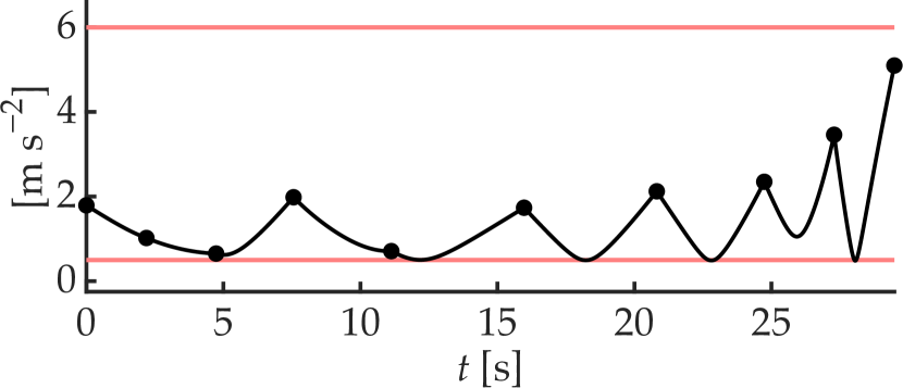
Trajectory optimization methods can be broadly classified into indirect and direct methods [4, Sec. 4.3]. Invoking the maximum principle to solve optimal control problems with general nonlinear dynamics subject to path constraints is challenging. Such solution methods, i.e., indirect methods, usually take an optimize-then-discretize approach, and can only handle a restricted class of problems. The solutions they generate, however, naturally ensure continuous-time feasibility [5, 6]. Methods that take the discretize-then-optimize approach, i.e., direct methods, on the other hand, are capable of handling general optimal control problems and are more reliable numerically (they are less sensitive to initialization). Since discretization is a crucial step in direct methods, the resulting solutions invariably suffer from so-called inter-sample constraint violations [7] (see Figure 1).
A majority of the existing direct methods, such as MISER [8], DIRCOL [9], PSOPT [10], PROPT [11], and GPOPS-II [12], transcribe optimal control problems to nonlinear programs (NLP) and call standard NLP solvers, such as SNOPT [13], IPOPT [14], and Knitro [15], which require second-order information, lack convergence guarantees, and are unsuitable for real-time, embedded applications. In contrast, software such as acados [16] and ACADO [17] interface with custom quadratic programming (QP), sequential quadratic programming (SQP), and NLP solvers that exploit the structure of the underlying problem. However, they neither guarantee convergence nor enforce continuous-time constraint satisfaction.
Several direct methods either—(i) assume a discrete-time formulation with path constraints imposed at finitely-many time nodes, i.e., they disregard the conversion of continuous-time problem descriptions to discrete-time ones (e.g., TrajOpt [18], PANOC [19, 20], CALIPSO [21]); (ii) provide convergence guarantees by restricting the class of path constraints [22, 23, 24, 25, 26, 27]; or (iii) ensure continuous-time constraint satisfaction for a restricted class of dynamical systems [28, 29, 30, 7].
Sequential convex programming (SCP) algorithms for trajectory optimization have received attention in the recent years [31, 2] as a competitive alternative to sequential quadratic programming (SQP) and IPM-based NLP algorithms, especially since SCP is a multiplier-free method and does not require second-order information. In trajectory optimization, computing the second-order sensitivities of nonlinear dynamics (which form a part of the Hessian of the Lagrangian within SQP and IPM) is expensive [32]. Recent work has explored convergence guarantees for SCP, in the context of both trajectory optimization [26, 33, 34, 35, 36, 37] and general nonconvex optimization [38, 39, 40, 41, 42]. SCP-based trajectory optimization methods, without theoretical guarantees, have been applied to a wide range of robotics and aerospace applications, with domain-specific heuristics that ensure effective practical performance [18, 43, 44, 45]. Widespread adoption of SCP for performance- and safety-critical applications, however, will necessitate the development of a general framework with rigorous certification of its capabilities.
We propose successive convexification, an SCP-based, real-time-capable solution method for nonconvex trajectory optimization, with continuous-time feasibility and guaranteed convergence. The proposed framework combines several key methods to solve a large class of nonlinear optimal control problems: (i) exterior penalty-based reformulation of the path constraints; (ii) generalized time-dilation; (iii) multiple-shooting discretization; (iv) exact penalization of the nonconvex constraints; and (v) the prox-linear method, an SCP algorithm for convex-composite minimization.
The reformulation of path constraints involves integrating the continuous-time constraint violation using a smooth exterior penalty, which is transformed into an auxiliary dynamical system with boundary conditions. The reformulation combined with multiple-shooting discretization [46] enables continuous-time feasibility even on sparse discretization grids, and obviates the need for mesh refinement heuristics. While such constraint reformulations have appeared in the optimal control literature since the 1960s [47, 48, 49] with specific choices of penalty functions [50, 51], the full extent of its capabilities for enabling SCP-based convergence-guaranteed, continuous-time-feasible trajectory optimization have not been explored, to the best of the authors’ knowledge. We address the consequences of the reformulation on a constraint qualification that is important in numerical optimization, and provide a rigorous quantification of the extent of continuous-time constraint satisfaction.
Through the prox-linear method [42, 52], we guarantee convergence of the solution method to stationary points of the -penalized problem and guarantee that the converged solutions that are feasible with respect to the discretized and control-parameterized optimal control problem are also Karush-Kuhn-Tucker (KKT) points. Furthermore, we highlight the specialization of this property to global minimizers of convex optimal control problems, wherein the reformulated path constraints cannot be represented by canonical cones, i.e., in the form required by existing convex optimization solvers.
In addition to theoretical analysis, we demonstrate the effectiveness of the proposed framework with numerical examples based on popular optimal control applications: two nonconvex problems—dynamic obstacle avoidance and 6-DoF rocket landing, and one convex problem—3-DoF rocket landing using lossless convexification. We also demonstrate the real-time capability of the proposed framework on the nonconvex examples considered, by executing C code generated using sc vx gen, an in-house-developed general-purpose real-time trajectory optimization software with customized code-generation support. The C codebase generated by sc vx gen uses the proposed framework to solve the optimal control problem at hand.
Simplified implementations of the proposed framework were recently demonstrated for specific applications, ranging from GPU-accelerated trajectory optimization for six-degree-of-freedom (6-DoF) powered-descent guidance [53] and nonlinear model predictive control (NMPC) for obstacle avoidance [54], to trajectory optimization for 6-DoF aircraft approach and landing [55].
2 Problem Formulation
This section describes the transformation of a path-constrained, free-final-time optimal control problem to a fixed-final-time optimal control problem through generalized time-dilation and constraint reformulation. The constraint reformulation involves the conversion of path constraints into a two-point boundary value problem for an auxiliary dynamical system.
2.1 Notation
We adopt the following notation in the remainder of the discussion. The set of real numbers is denoted by , the set of nonnegative real numbers by , the set of real matrices by , and the set of real vectors by . The concatenation of vectors and is denoted by , the concatenation of matrices and by , the Cartesian product of sets and by , and the Kronecker product by . The vector of ones in is denoted by , the identity matrix in by , and the matrix of zeros in by . Whenever the subscript is omitted, the size is inferred from context. For any scalar , we define . The operations , , (and their compositions) apply elementwise for a vector. The Euclidean norm of a vector is denoted by . The indicator function of a convex set is denoted by (see [56, E.g. 3.1]), and its normal cone at by [57, Def. 5.2.3]. The subdifferential of a function , evaluated at , is a set denoted by , and its members are called subgradients. The gradient of a differentiable function with respect to , evaluated at , is denoted by , where the elements of can include a subset or superset of the arguments of (irrespective of the order), and the subscript is omitted if it coincides with the list of arguments of . The (sub)gradient of a scalar-valued function at a point is defined to be a row vector (for e.g., from ). The (sub)gradient of a vector-valued function is a matrix consisting of the (sub)gradients of its scalar-valued elements along the rows. In particular, the partial derivatives of function , evaluated at , are denoted by , , respectively (with the argument inferred from context whenever omitted). Furthermore, the notation represents the derivative with respect to a scalar variable.
2.2 Optimal Control Problem
We consider a class of free-final-time optimal control problems for nonlinear dynamical systems with nonconvex constraints on the state and input, given by
where the derivative with respect to time in (1b) is denoted by . We assume that the terminal state cost function , the dynamics function , the path constraint functions , , and the boundary condition constraint functions , are continuously differentiable. The inequality and equality constraints in (1c)-(1f) are interpreted elementwise. The initial time is fixed, while the final time is a free (decision) variable. For simplicity, we omit parameters [2, Eq. 1] of the system dynamics and constraints in (1). With minimal modifications, the subsequent development can handle parameters as decision variables as well. Note that the above problem can be a nonconvex trajectory optimization problem due to: i) nonlinear dynamics, i.e., is a nonlinear function; ii) final time being free; iii) nonlinear functions and ; iv) nonconvex functions and .
We assume that the control input is a piecewise continuous function. Since is continuously differentiable, this ensures the existence and uniqueness of an absolutely continuous function , the state trajectory, which satisfies (1b) almost everywhere and the following integral equation
where is the initial state. Note that existence and uniqueness of the state trajectory can be ensured with weaker assumptions; we refer the reader to [58, Sec. 3.3.1] and [59, Sec. II.3] for detailed discussions. We also require the following boundedness assumption based on Gronwall’s Lemma [60, Chap. 4, Prop. 1.4].
Assumption 1.
For any compact and , there exist positive and such that for all .
Note that Assumption 1 may not always hold. Consider . For any positive and , when becomes sufficiently large, Assumption 1 is invalid. Nonetheless, for physical systems, one can define a compact set , containing all physically meaningful states. Any state not contained in can be regarded as infeasible. Consequently, we create a modified dynamics function so that it satisfies Assumption 1 and is consistent with the original dynamics function on . To be precise, for any open set containing , there exists a smooth function such that for all and the support of is compact and contained in , as shown in [61, Thm. 8.18]. Therefore, we can replace function in (1b) with , which is compactly supported in , ensuring Assumption 1. Note that the inclusion of is only for the purpose of proofs of results discussed in subsequent sections; it is not necessary in a practical implementation.
The optimal control problem (1) is posed in the Mayer form [58, Sec. 3.3.2], without loss of generality. The original problem could be provided in the Bolza or Lagrange forms where the objective function contains the integral of a continuously differentiable running cost function , given by
which is well-defined when is a state trajectory and is the corresponding piecewise continuous control input. The Mayer form is obtained from the Lagrange and Bolza forms by equivalently reformulating the integral of as a new dynamical system
| (2) |
and adding as a terminal state cost to the objective function, along with specifying the initial condition .
We propose an SCP and multiple-shooting based solution method [46] (which only requires first-order information). The gradient of the integral of can be computed through the first-order sensitivities [62, Sec. 4.2] of dynamical system (2)—a qualitatively similar effort to linearizing (1b). Therefore, converting to the Mayer form is beneficial for consolidating majority of the effort of gradient computation in one place, which is efficient for numerical implementations. Furthermore, the integral of running cost function can be either convex or nonconvex. In the convex case, however, the integral often cannot be reformulated as a canonical conic constraint with the help of additional slack variables (see Section 5.1 for further details). Moreover, a convex running cost function in a free-final-time problem will become nonconvex after conversion to a fixed-final-time problem via the time-dilation technique described in Section 2.4. In the subsequent development, unless stated otherwise, we assume that the dynamical system (1b), the terminal state cost function , and the boundary condition (1f) already encode any desired running cost terms.
2.3 Constraint Reformulation
To reformulate path constraints (1c) and (1d), we consider continuous exterior penalty functions
| (3a) | |||
| (3b) | |||
| (3c) | |||
| (3d) | |||
and the penalty function
| (4) |
Note that , , and , , denote the scalar-valued elements of functions and , respectively. It is straightforward to show that is piecewise continuous over when is a state trajectory and is the corresponding piecewise continuous control input.
Proof:
For each , is nonnegative since and are nonnegative. Since is piecewise continuous, (5) holds iff .
Then, and , which is equivalent to and .
Next, we augment the system dynamics with an additional state to accumulate the constraint violations, and impose periodic boundary conditions on it to ensure continuous-time constraint satisfaction.
Corollary 3.
The differential-algebraic system
| (6a) | |||
| (6b) | |||
| (6c) | |||
is satisfied by and a.e. in iff and solve the boundary value problem on
| (7a) | ||||
| (7b) | ||||
| (7c) | ||||
Proof: Suppose that and satisfy (1b), (1c), and (1d) almost everywhere in . Since is piecewise continuous over , there exists a unique state trajectory which satisfies (7b) almost everywhere in with initial condition . Then, iff (5) holds. Therefore, from Lemma (2), the path constraints (1c) and (1d) are satisfied almost everywhere in .
For the other direction, we let , , and be the solution to (7). Then, (7c) implies that (5) holds. We obtain the desired result from Lemma 2.
Remark 4.
Since a gradient-based solution method will be adopted, the exterior penalty functions and , for and , must be continuously differentiable in order to compute first-order sensitivities [62, Sec. 4.2] of (7b). For e.g.,
| (8) |
for any , are valid choices. Then, can be compactly written as
| (9) |
for any , , and .
Remark 5.
Remark 6.
The penalty function can be defined more generally as a vector-valued function of the form
| (13) |
for any , , and , where matrix , which we refer to as the mixing matrix, has nonnegative entries, and functions and are defined as
| (14a) | ||||
| (14b) | ||||
for any and , with and . The mixing matrix has at most rows, at most one positive entry per column, and exactly positive entries in total. We obtain (4) and a scalar-valued state in (7b) by choosing . In general, choosing (13) will lead to a vector-valued state for quantifying the total constraint violation. While (4) is suitable for most cases, choosing (13) for certain applications can be numerically more reliable. In the remainder of the discussion, we adopt the definition in (4). However, the results also apply to the general representation in (13).
2.4 Generalized Time-Dilation
Time-dilation is a transformation technique for posing a free-final-time optimal control problem as an equivalent fixed-final-time problem [44, Sec. III.A.1]. Let be a state trajectory for (1b) over obtained with control input and some initial condition. We define a strictly increasing, continuously differentiable mapping , with boundary conditions , and treat the derivative of the map
for , as an additional control input, which we refer to as the dilation factor. Note that the derivative with respective is denoted by . Previously, dilation factors were either treated as a single parameter decision variable (as in [44, Sec. III.A.1]) or multiple discrete parameter decision variables (as in [63, Sec. 2.1]). The approach proposed herein generalizes it by treating dilation factor as a continuous-time control input. We note that this approach bears resemblance to the time-scaling transformation proposed in [64, 65]. Further, we treat as an additional state, and define functions and as
| (15a) | |||
| (15b) | |||
for . Then, using chain-rule, we obtain
| (16) |
for , where
| (17) |
We refer to (16) as the augmented system, with augmented state , and augmented control input .
In the subsequent development, we define and use matrices , , and to select the first elements (), the penultimate element (), and the last element (), respectively, of . Similarly, matrices and select the first elements () and the last element (), respectively, of . Note that generalized time-dilation transforms non-autonomous dynamical systems into equivalently autonomous ones (without explicit dependence on time) by increasing the dimensions of the state and control input. If the final time is fixed in (1), then the generalized time-dilation step can be skipped. Henceforth, we drop the qualifier “generalized” for brevity.
Remark 7.
When the system dynamics and constraint functions in (1) are time-varying, we use time-dilation to augment the system with an extra state and control input. However, when the system and constraint descriptions are time-invariant, it suffices to augment only the control input.
2.5 Reformulated Optimal Control Problem
Subjecting (1) to constraint reformulation and time-dilation results in the following optimal control problem
where,
| (19a) | ||||
| (19b) | ||||
| (19c) | ||||
for any . Since time is treated as a state variable, its initial condition needs to be specified through . This is not needed in (1) because (constant) is explicitly passed to functions and . Furthermore, positivity of the dilation factor is ensured using (18c). Observe that, as a consequence of the constraint reformulation, the continuous-time constraints on the state and control input are not explicitly imposed in (18); they are instead embedded within the augmented system in (18b) and boundary condition (18d).
3 Parameterization and Discretization
This section describes the transformation of the (infinite-dimensional) reformulated optimal control problem (18) into a (finite-dimensional) nonconvex optimization problem through parameterization of the augmented control input, and discretization of (18b) over the interval . In addition, we introduce a relaxation to the constraint reformulation step after discretization to ensure favorable properties from an optimization viewpoint, and analyze the consequences of the relaxation.
We parameterize the augmented control input with finite-dimensional vectors via , defined as
| (20) |
for , where
| (21) |
Each element in (21), , is a polynomial basis function, for and . Vectors and , which are the decision variables, are coefficients parameterizing the control input and dilation factor. The support of each of the basis functions in and can be pairwise disjoint and strictly contained in .
| (22) |
Remark 8.
The parameterization (20) for the augmented control input is general enough to subsume several control input parameterizations used in practice, such as zero- and first-order-hold, and pseudospectral polynomials in orthogonal collocation (see Appendix B). We distinguish between the parameterizations for the control input and dilation factor because the former is allowed to have a general polynomial parameterization as long as is elementwise bounded, whereas, the latter must be constrained to be bounded and positive due to (18c). Such a requirement should be straightforward to handle with convex constraints on .
After parameterizing the augmented control input, we discretize (18b) via its integral form over a finite grid of size in , denoted by . We treat the augmented states at the node points also as decision variables, and denote them compactly as
Next, we define
| (23) | |||
for , where the augmented state trajectory satisfies (18b) almost everywhere on with augmented control input , and initial condition . Then, the discretization of (18b), together with (18d), yields the constraints
| (24a) | |||
| (24b) | |||
for . The discretization in (24a), commonly referred to as multiple-shooting, is exact because there is no approximation involved in switching to the integral representation of the differential equation (18b), and it is numerically more stable compared to its precursor, single-shooting [5, Sec. VI.A.3].
Definition 9 (Continuous-Time Feasibility).
The triplet , , and is said to be continuous-time feasible if it satisfies (24).
A continuous-time feasible triplet: , , and corresponds to an augmented state trajectory generated by integration of over with augmented control input and initial condition , such that it passes through the node values at , for . Furthermore, due to (24b), the resulting state trajectory and control input satisfy the path constraints almost everywhere in .
Continuous-time feasibility is a crucial metric for assessing the quality of solutions computed by direct methods. They solve for finite-dimensional quantities (such as , , and ) which parameterize the control input, and at times, even the state trajectory. In particular, direct collocation methods [6] approximate the state trajectory with a basis of polynomials (for e.g. orthogonal collocation methods [66, 67]). They match the derivative of the polynomial approximant to the right-hand-side of (1b), and impose the path constraints at finitely-many nodes. As a result, such methods cannot guarantee that the computed solution is continuous-time feasible, necessitating computationally intensive heuristics such as mesh refinement [4, Sec. 4.7]. On the other hand, the proposed framework leverages multiple-shooting and constraint reformulation to provide continuous-time feasible solutions, which is a key distinction compared to existing direct methods [1, Sec. 2.4.1], [68, Table 1.1].
3.1 Constraint Qualification and Relaxation
An issue with directly imposing (24) is that it violates linear independence constraint qualification (LICQ) [69, Def. 12.4]. For each point in , we can determine the active set [69, Def. 12.1] corresponding to the constraints in (24). LICQ is said to hold at a point if the gradients of the constraints in the corresponding active set are linearly independent. The following result shows that LICQ is violated at all points feasible with respect to (24).
Proof: Suppose , , and satisfy (24a) and (24b). For each , let be the augmented state trajectory on with augmented control input and initial condition . Then, due to Lemma 2, path constraints (1c) and (1d) are satisfied almost everywhere on the time interval . Recall that defined in (17) is continuously differentiable and that is piecewise continuous. This implies that
are piecewise continuous functions. Therefore, they are integrable and the partial derivatives of are well-defined. Elements of the penultimate row of and (i.e., the partial derivatives of ), are zero on when evaluated on and . This is because all elements of this row contain factors of the derivatives of or , which are zeros due to Remark 5. Hence, only the partial derivatives of with respect to and contain nonzero elements in that row, as shown in (25a) and (25b).
Using Lemma 25, for any , , and satisfying (24a) and (24b), the gradient of the left-hand-side of (24b), and the penultimate row of the gradient of (shown in (25)) are identical. Hence, all feasible solutions of an optimization problem having both (24a) and (24b) as constraints will not satisfy LICQ. The proposed framework relies on the classical exact penalization result to determine KKT points of (26) [69, Thm. 17.4], which are related to local minimizers when LICQ holds [69, Thm. 12.1]. So, we remedy the pathological scenario due to (24) by relaxing (24b) to an inequality with a positive constant .
Then, (18) transforms under augmented control input parameterization (20) and discretization (24) as follows
where and are compact convex sets.
Remark 11.
If , , and satisfy (26b) and (26c), then LICQ will not be trivially violated by the active set associated with (26c) and the penultimate row of (26b). If (26c) holds with strict inequality, for all , then the result follows immediately. However, if for some , (26c) holds with equality, then
| (27) |
where is the augmented state trajectory with augmented control input and initial condition . Due to piecewise continuity of the integrand in (27) with respect to , it implies that there exists an interval where the integrand of (27) is positive, i.e., some of the path constraints are violated on the segments of and corresponding to interval . Therefore, unlike the case in Lemma 25, the partial derivatives of evaluated on those segments of and will not be trivially zero.
Remark 12.
Besides addressing the LICQ issue, relaxation (26c) is essential for enabling exact penalization—a key step in the proposed framework. The combination of (24a) and (24b) is equivalent to the following constraint for each
| (28) |
Exact penalization of (28) involves penalizing the left-hand-side of (28) using a nonsmooth exterior penalty function (such as ). However, the effect of exterior penalty is suppressed due to the positivity and continuous differentiability of , which destroys the exactness of the penalty term (see discussion in [69, p. 513]). In other words, it may not be possible to recover a solution that is feasible with respect to (28) using a finite weight for the penalty term.
Remark 13.
Set ensures that the control input lies in a compact convex set. Whenever the choice of parameterization permits (e.g., with zero- or first-order-hold), the convex control constraints in (1c) and (1d) could be captured with , i.e., via imposing convex control constraints only at the node points (inter-sample constraint satisfaction is guaranteed); otherwise, will encode elementwise bounds on . Set ensures that the dilation factor is positive and bounded. Besides handling convex control constraints directly, requiring the augmented control input to lie in a compact set via (26d) is necessary for deriving a pointwise constraint violation bound, given the -relaxation in (26c).
3.2 Gradient of Discretized Dynamics
A key step in any gradient-based solution method for (26) is to compute the partial derivatives of . We adopt the so-called variational method [65, Sec. 3.2], [62, Sec. 4.2], also referred to as inverse-free exact discretization [63, Sec. 2.3].
Let , , and denote a reference solution, and let denote the corresponding parameterization using (20). For each , consider the following initial value problem over
| (29a) | |||
| (29b) | |||
| (29c) | |||
| (29d) | |||
| (29e) | |||
| (29f) | |||
where , , and , for . The partial derivatives of evaluated on the augmented state trajectory for (18b) over , with augmented control input and initial condition , are compactly denoted with , , and , i.e.,
| (30a) | ||||
| (30b) | ||||
| (30c) | ||||
for . Then, the partial derivatives of with respect to , , and (denoted by , , and ) evaluated at the reference solution are related to the terminal value of the solution to (29) as follows
| (31a) | ||||
| (31b) | ||||
| (31c) | ||||
Finally, the linearization of is given by the mapping
| (32) | |||
Note that arbitrarily chosen , , and are, in general, not continuous-time feasible, i.e., , for . We refer to [70, Sec. II] and [63, Sec 2.3] for further insights and related methods for discretization and linearization of nonlinear dynamics.
3.3 Pointwise Constraint Violation Bound
Given a solution for (26), we can obtain the state trajectory , control input , and final time . In addition, we can construct a time grid , satisfying and . Node is the time instant corresponding to , for . The length of interval is denoted by , for , and denotes a lower bound for the lengths of the intervals. Then we can establish an upper bound for the pointwise violation of the path constraints when (26c) is satisfied for a specified , and with the choice of exterior penalties (8).
Theorem 14.
Proof: See Appendix A.
While the analysis in Appendix A assumes (8), other valid exterior penalty functions can be handled in a similar manner. Further, note that the bound in (33) is consistent because is strictly monotonic for and as , where . We can use these bounds to select an that is numerically significant yet physically insignificant for the underlying dynamical system and constraints.
Remark 15.
The pointwise bound for the inequality path constraints specifies the amount of constraint tightening required for the solutions obtained with relaxation (26c) to satisfy the constraints with no pointwise violation. More precisely,
We cannot, however, specify such a tightening for the equality constraints that ensures pointwise satisfaction. We can only control the extent of pointwise violation using (62). Specialized techniques such as the one proposed in [71] could be explored as a future direction.
Remark 16.
The estimate of and can be conservative whenever it is challenging to tightly bound . As a result, the bound in (33) can become conservative. In such cases, a solution to (26) can be iteratively refined until the pointwise violations are within a desired tolerance. We can successively solve (26) by reducing by a constant factor and warm-starting with the previous solution. This refinement process will terminate since is strictly monotonic and consistent (i.e., ).
The key distinction between the approach in Remark 16 and the mesh refinement techniques for alleviating inter-sample constraint violation [72, 73, 74] is that the former does not add more node points to the discretization grid, i.e., remains fixed. The proposed framework can achieve continuous-time constraint satisfaction (up to a tolerance ) on a sparse discretization grid. Most direct methods verify the extent of inter-sample constraint violation a posteriori, i.e., after solving the trajectory optimization problem for a chosen discretization grid. In contrast, the proposed framework specifies the extent of allowable inter-sample constraint violation within the optimization problem.
4 Prox-Linear Method for Numerical Optimization
We propose a solution method which applies an SCP algorithm called the prox-linear method [40, 42] to an unconstrained minimization obtained from transforming (26) via exact penalization of (26b) and (26e) [69, Eq. 17.22].
4.1 Exact Penalization
We can construct an unconstrained minimization problem from the constrained problem (26) by penalizing the constraints. The penalty terms have weights as tunable hyperparameters in the unconstrained problem. The penalty functions are said to be exact whenever, for a finite penalty weight, the stationary points and local minimizers of the unconstrained problem can capture the KKT points and local minimizers of the constrained problem. A widely-used example of such penalty functions, which are typically nonsmooth, are the penalty functions [69, Eq. 17.22]. Quadratic penalty functions, in contrast, are not exact, i.e., the penalty weight must tend to infinity in order to obtain the first-order optimal points of the constrained problem. Clearly, adopting an exact penalization of constraints is practical for designing a numerical solution method since the solution to a single unconstrained problem can deliver a solution to the original constrained problem without needing to solve a sequence of problems where penalty weight is arbitrarily increased.
Standard results on exact penalization [75, 76, 77], [69, Chap. 17] for general constrained optimization appeared close to three decades ago, and are widely used. However, they don’t directly apply for the proposed formulation since the construction of (26) is atypical, in that it possesses convex constraints: (26c), (26d) (represented with convex sets), and nonconvex constraints: (26b), (26e) (represented with functions). While transforming (26) into an unconstrained minimization, we wish to subject only the nonconvex constraints to exact penalization, while using indicator functions to represent the convex constraints, so that they can be directly parsed without approximations to a conic optimization solver iteratively called within the prox-linear method. The standard exact penalty results cannot be directly applied to this hybrid case. To the best of authors’ knowledge, an exposition on the modifications necessary to handle the hybrid case is not available in the literature. For completeness and clarity, this section presents the exact penalty results with required modifications along with the proofs.
Given , function is defined as
where , , , and is a closed convex set with
The -penalization of constraints (26b) and (26e) involves penalty functions and , respectively.
Our goal then is to compute a local minimizer of where the penalty terms are zero. We start by seeking a stationary point of , since local minimizers are stationary points. Determining stationary points is a relatively simpler task than directly attempting to solve the nonconvex problem (26). We can rewrite the indicator function for as explicit convex constraints111Commonly encountered convex sets such as polytope, ball, box, second-order cone, halfspace, hyperplane etc. can be directly represented in conic optimization solvers, such as ECOS [78] and MOSEK [79], as the intersections of canonical cones: zero cone, nonnegative orthant, second-order cone, and the cone of positive semidefinite matrices. while computing a stationary point of via SCP. A stationary point satisfies , i.e., there exists and denoted by
| (36) | ||||
with , such that
| (37) | ||||
where with . The scalar-valued functions , , and are elements of , , and , respectively, indexed by . The gradients of , , and are with respect to . The convex subdifferential of and are
| (38d) | ||||
| (38h) | ||||
for any . We refer the reader to [52, Sec. 3.2] and the references therein, for the definition and properties of the subdifferential of a nonconvex function.
Next, we need the following lemma about the normal cone of a convex set.
Lemma 17.
Suppose that , convex set is defined with continuously differentiable convex functions , and convex set is defined with vectors and scalars . Assume that 1) the collection of vectors , for , and , for are linearly independent, where is an index set, and 2) the intersection of and the interior of is nonempty. Then, we have
| (39a) | ||||
| (39b) | ||||
| (39c) | ||||
where the set addition in (39c) is a Minkowski sum.
Proof: The construction of and follow directly from [80, Thm. 10.39, Cor. 10.44, Thm. 10.45], and the expression for is derived from [81, E.g. 3.5] and [80, Thm. 4.10], where we use the fact that for any , where , .
Remark 18.
Given a convex optimization problem with a feasible set described by in Lemma 17, the corresponding assumptions are regularity conditions similar to LICQ and strong Slater’s assumption [57, Def. 2.3.1], which are typically needed for a well-posed convex optimization problem. We require the assumptions in Lemma 17 on convex set since the SCP approach will involve a sequence of convex problems with as the feasible set.
Theorem 19.
Proof: Suppose that is feasible with respect to (26), where with . Note that is a KKT point of (26) if and only if there exists (using Lemma 17) and such that
| (40) |
and
| (41) |
for . Similar to (37), the gradients of , , and in (40) are with respect to .
If is a stationary point of , then there exists and such that (40) holds, where
| (42) | ||||
The arguments of , , and , which are elements of , are omitted in (42) for brevity. Observe that satisfies (41) due to the feasibility of for (26) and due to the definition of in (38). Therefore, is a KKT point of (26).
Conversely, if is a KKT point of (26), then there exists and such that (40) and (41) hold. Note that is feasible with respect to (26) and suppose that . Then, we obtain , for , and , for , . Furthermore, for , we have the following. If , then . Alternatively, if , then , i.e., .
Next we relate the local minimizers of (26) to the stationary points and local minimizers of .
Theorem 20.
Proof: Consider a modification of , denoted by , where convex constraints due to are also -penalized instead of using the indicator function. The first statement follows from Theorem 4.4 in [75] if we first replace with , and note that with equality iff . The last statement follows from Propositions 3.1 and 3.3 in [76].
Stronger versions of the exact penalization results also exist. For instance, it can be shown under certain assumptions that, given a local minimizer of (26), there exists a neighborhood around it where the stationary points of are also local minimizers of (26). We refer the reader to [77] for further details.
4.2 Prox-Linear Method
We use the prox-linear method [42, Sec. 5] developed for convex-composite minimization to compute stationary points of . The prox-linear method is applicable when can be fit into the following template
| (43) |
where is a proper closed convex function, is an -Lipschitz continuous convex function, and is potentially nonconvex and continuously differentiable with a -Lipschitz continuous gradient.
The prox-linear method finds a stationary point of by iteratively minimizing a convex approximation for given by
| (44) | |||
where is the current iterate, with , and determines the proximal term weight. The nonconvex term is convexified by linearizing at . We denote the unique minimizer [56, Sec. 9.1.2] of the strongly convex function as . The iterative minimization of amounts to solving a sequence of convex subproblems, which is numerically very efficient and reliable. The convergence of this iterative approach is quantified using the prox-gradient mapping
This is because iff is a stationary point of [52, Sec. 3.3]. Observe that defined in (35) fits the template of (43): the terminal cost function and the exact penalties for , , and are represented by the composition , and the indicator function is represented by . More precisely, for any , we choose
| (45a) | ||||
| (45b) | ||||
| (45c) | ||||
where with , , , and . While minimizing (44), we translate into explicit convex conic constraints that can be handled by convex optimization solvers such as ECOS [78], MOSEK [79], and PIPG [82].
Lemma 21.
Under Assumption 1, the gradients of , , , and are bounded on on .
Proof: Functions , , , and are continuously differentiable. The domain of is . From Assumption 1 and [60, Chap. 4, Prop. 1.4], state trajectories generated with a bounded control input and dilation factor (due to (26d)) are bounded. Boundedness of the dilation factor also ensures that is bounded. Then, there exists a constant, , that bounds the norm of the gradients of , , , and on .
Figure 3 shows the complete solution method that we propose, and Algorithm 1 describes the prox-linear method. The inputs to the algorithm are the maximum number of iterations, , the termination tolerance, , and the proximal term weight, . Note that the “Convexification” block in Figure 3 constructs the subproblem based on (44), which forms a convex approximation of the composition . Since the convex approximation is non-affine based on our choice of , we call this step “Convexification” rather than “Linearization”. Furthermore, this step computes the gradient of the discretized dynamics (24a), as described in Section 3.2.
We have the following result about the monotonic decrease of for a sufficiently small .
Theorem 22 (Lemma 5.1 of [42]).
The magnitude of is both a practical and rigorous measurement for assessing whether is close to a stationary point (see [42, Thm. 5.3] for details). We then have the following finite-stop corollary.
Corollary 23.
Suppose is bounded below by and . For a given tolerance , prox-linear method achieves
Remark 24.
In practice, can be computed by either implementing a line-search as described in [42, Alg. 1] or by adopting the adaptive weight update strategy in [41, Alg. 2.2], where the equivalence between the trust-region and prox-linear methods is also discussed. The “Update Hyperparameters” block in Figure 3 represents the use of such update techniques. The implementation of the prox-linear method can be further enhanced using the acceleration scheme described in [52, Sec. 7].
Note that the upper bound for in Theorem 22 is a sufficient condition for convergence to a stationary point. In general, if the prox-linear method converges with arbitrary user-specified weights and , then the converged solution is guaranteed to be a stationary point, due to [42, Thm. 5.3].
Remark 25.
The prox-linear method is susceptible to the crawling phenomenon exhibited by SCP algorithms [83], wherein the iterates make vanishingly small progress towards a stationary point when they are not close to one. This phenomenon can happen when is chosen to be very large, which decreases the upper bound on for ensuring monotonic decrease of . Then, the lower bound for becomes very small even if is not small. The crawling phenomenon can be remedied by scaling the decision variables and the constraint functions so that their orders of magnitude are similar.
Remark 26.
The penalized trust region (PTR) SCP algorithm in [44, 84] solves a sequence convex subproblems similar to the ones generated by the prox-linear method. The PTR algorithm also implements a class of time-dilation, discretization, and parameterization operations to the optimal control problem (1), albeit in an order that is different from what we propose. The resulting sequence of convex subproblems that PTR solves can fit within the template of (43) after minor modifications. The weights of the proximal and exact penalty terms are heuristically selected to obtain good convergence behavior.
In summary, the proposed framework based on the prox-linear method globally converges to a stationary point of (Theorem 22), and if the stationary point is feasible with respect to (26), then it is a KKT point (Theorem 19). Furthermore, each strict local minimizer of (26) with LICQ satisfied is a local minimizer of for a large-enough finite (Theorem 20).
5 Exploiting Convexity
Next we consider optimal control problem (1) where both initial and final times , are fixed, the terminal cost function is convex in the terminal state, the dynamical system (1b) is a linear nonhomogeneous ordinary differential equation, represented by
| (46) |
for , and the constraint functions in (1c), (1d), (1e), and (1f) are jointly convex in all arguments (except time). In particular, constraint functions and are affine in state and control input. Furthermore, we deviate from the Mayer form by explicitly specifying a running cost term in the objective with a continuously differentiable function that is jointly convex in the state and control input. Embedding the running cost into the dynamics, as mentioned in Section 2.2, would turn the dynamical system nonlinear and hence destroy the convexity of the optimal control problem.The resulting optimal control problem is now in the Bolza form [58, Sec. 3.3.2].
To obtain a finite-dimensional optimization problem similar to (26), we first parameterize the control input and discretize (46). Time-dilation is not necessary in the fixed-final-time setting, and constraint reformulation is postponed to the end with a minor modification to exploit convexity of the constraints. We apply parameterization (20) directly to the control input in the time domain, i.e., , for . To discretize (46), we form a grid of size in denoted by , and treat the states at node points as decision variables. Then, for each , we exactly discretize (46) via the integral form into
| (47) |
for , where state trajectory generated with control input and initial condition satisfy (46) . Moreover, , , and are computed as the solution to an initial value problem222Note that, unlike in (29), superscript “” is absent from , , and since they are independent of the state trajectory . similar to (29), and we denote their terminal values as , , and .
Next, the path constraints (1c) and (1d) are reformulated as follows. For each , define and by substituting in the control parameterization and the discretized form (47) into and
| (48) | |||
where . Note that each scalar-valued element of and is jointly convex in and . Then, for each , we obtain
| (49a) | |||
| (49b) | |||
where is defined as
Similar to (26c), we need to relax (49b) with in order to facilitate exact penalization.
Lemma 27.
is a convex function.
Proof: Observe that is a convex, non-decreasing function. Then, the composition is a convex function [56, Sec. 3.2.4]. Furthermore, is a sum of convex quadratics of its arguments since is an affine function.
For each , the running cost over can be compactly expressed with function by substituting in the control parameterization and the discretized form (47) as
| (50) |
where is a state trajectory for (46) over , generated with control input and initial condition .
Finally, we obtain the convex optimal control problem subject to parameterization, discretization, and reformulation (49b) of path constraints with -relaxation.
where and the compact convex set plays a role similar to that in Remark 13.
Although is a convex constraint, we do not possess any structural or geometric information needed to classify it as a conic constraint of the form , where is a Cartesian product of canonical convex cones: zero cone, nonnegative orthant, second-order cone, cone of positive semidefinite matrices etc. In fact, we only have access to first-order oracles for and that provide the function value and its gradient at a query point. As a consequence, we cannot directly use existing conic optimization solvers [78, 85, 79] to solve (51).
We adopt the prox-linear method after exactly penalizing (51c), since it is compatible with the first-order oracles for and . Convexity of (26) guarantees global convergence to the set of minimizers.
Besides incorporating the -relaxation in (51c) to facilitate exact penalization, we also assume that representation (51b)-(51f) for the feasible set of (51) satisfies the strong Slater’s assumption [57, Def. 2.3.1]. This assumption is necessary and sufficient for the set of Lagrange multipliers associated with a minimizer of (51) to be nonempty, compact, and convex [57, Thm. 2.3.2].
5.1 Exact Penalization & Prox-Linear Method
Similar to (35), for a given , consider the convex function defined by
where and with
| (58) |
is the convex set encoding all state constraints except for (51c), which is subject to penalization. Note that when in (52), i.e., when (49b) is not subject to relaxation, then its penalization is not exact since leads to a quadratic penalty on the violation of path constraints.
Lemma 28.
Under Assumption 1, the gradients of and are bounded on .
Proof: The domain of is . Similar to Lemma 21, we can again invoke Assumption 1 and [60, Chap. 4, Prop. 1.4] to infer that a bounded control input parameterization (due to (51d)) generates bounded state trajectories over the time interval . Then, there exists a constant, , that bounds the norm of the gradients of and on .
Due to the convexity of (51), we can invoke a stronger exact penalization result than those in Section 5.1.
Theorem 29.
Proof: The result follows from [57, Cor. 3.2.3, Thm. 3.2.4]. Note that strong Slater’s assumption ensures that strong duality holds.
Theorem 30.
Proof: The monotonic decrease of (52) guaranteed by Theorem 22 when , together with Corollary 23 and [42, Thm. 5.3], implies that Algorithm 1 will get arbitrarily close to a stationary point in a finite number of iterations. Since stationary points of (52) are identical to the minimizers of (51), due to Theorem 29, we have that Algorithm 1 will get arbitrarily close to a minimizer of (51) in a finite number of iterations.
Even though prox-linear method will globally converge to a minimizer of (51), providing a good initial point will dramatically improve its practical convergence behavior. A solution to the closely related convex optimization problem where all path constraints are explicitly imposed as conic constraints at finitely-many time nodes will serve as a good initialization. Computing such a solution is very efficient in practice with existing convex solvers.
6 Numerical Results
We provide a numerical demonstration of the proposed framework with three examples: dynamic obstacle avoidance, six-degree-of-freedom (6-DoF) rocket landing, and three-degree-of-freedom (3-DoF) rocket landing with lossless convexification. The first two examples are nonconvex problems while the third one is convex. Appendices C through E describe the problem formulation (in the form of (1)) and the algorithm parameters for each of the examples. The results in this section are generated with code in the following repository
github.com/UW-ACL/successive-convexification
For all examples considered, the convex subproblems of prox-linear method are QPs, which are solved using PIPG [82]. We also demonstrate the real-time capability of the proposed framework by using a C codebase generated by sc vx gen, a general-purpose SCP-based trajectory optimization software with customized code generation, in tandem with ECOS [78].
The proximal term weight is determined using a line search and the exact penalty weight is determined by gradually increasing it by factors of (see the discussion in [2, p. 78]). Unless otherwise specified, the initial guess for the prox-linear method consists of a linear interpolation between the initial and final augmented states, and a constant profile for the augmented control input. The nodes of the discretization grid in for free-final-time problems, and in for fixed-final-time problems, are uniformly spaced. To ensure reliable numerical performance, all decision variables and constraint functions and are scaled [84, Sec. IV.C.2] to similar orders of magnitude. We refer the reader to [4, Sec. 4.8] for a discussion on the effects of scaling in numerical optimal control.
We compare solutions from the proposed framework with those from an implementation where path constraints are not reformulated (i.e., they are only imposed at the discretization nodes), which we refer to as the node-only approach. We demonstrate that the proposed framework can compute continuous-time feasible solutions on a sparse discretization grid without mesh-refinement, and that the node-only approach is susceptible to inter-sample constraint violation on the same sparse grid. Handling sparse discretization grids and eliminating mesh-refinement makes the proposed framework amenable to real-time applications. Moreover, the resulting state trajectory can activate constraints between discretization time nodes, which is a unique characteristic among other direct methods.
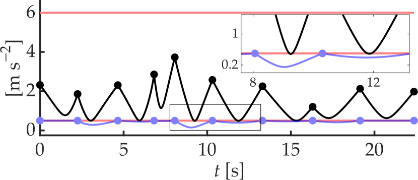
In the plots that follow, unless otherwise stated, we adopt the following convention. Dots denote the solution from prox-linear method: black () for proposed framework and blue () for node-only approach. Lines denote the continuous-time control input and state trajectory constructed using the solution from prox-linear method: black (-) for proposed framework and blue (-) for node-only approach. (We simulate/integrate (1b) with the parameterized control input to obtain the state trajectory.) Red lines (-) denote the constraint bounds. Inter-sample violation in the solutions from the node-only approach is highlighted with magnified inset.
6.1 Dynamic Obstacle Avoidance
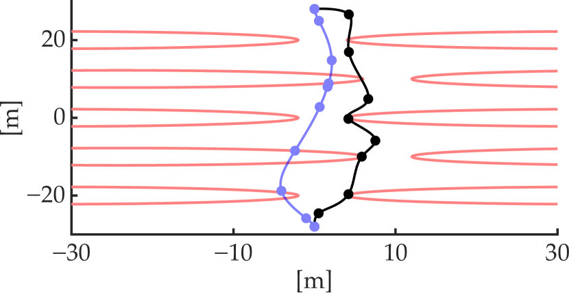
We consider two scenarios: one where the obstacles exhibit periodic motion and the other where they are static. Figure 4(a) shows the magnitude of control input (acceleration) in the case with dynamic obstacles obtained with the proposed framework. An animation of the corresponding position trajectory is provided in the code repository. A solution from the node-only approach is not shown in Figure 4(a), since it fails to provide a physically meaningful solution on the same discretization grid due to aliasing in the obstacle motion. Due to the time variation in the obstacle positions, a dense discretization grid is required with the node-only approach. However, the number of distinct obstacle avoidance constraints imposed in the node-only approach grows with the discretization grid size and the number of obstacles, which is computationally expensive. On the other hand, the number of constraints imposed in the proposed framework only depends on the discretization grid size.
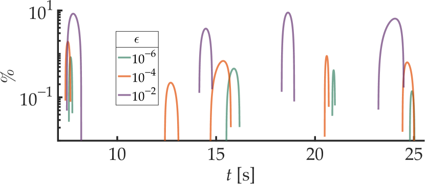
Figure 4(b) shows the percentage of violation in the obstacle avoidance constraint by the simulated state trajectories obtained for different values of the constraint relaxation tolerance . As long as the constraint functions are well-scaled, a state trajectory with physically insignificant continuous-time constraint violation can be obtained by picking to be several orders of magnitude greater than machine precision, which is essential for reliable numerical performance. In practice, picking close to ensures that the continuous-time constraint violation does not exceed .
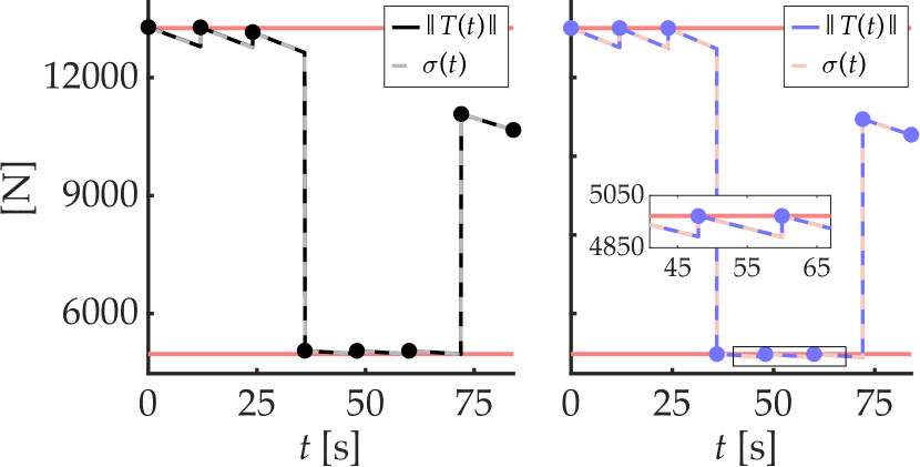
To compare the proposed and the node-only approaches, we turn to the case of static obstacles: Figure 5(a) shows the position and Figure 5(b) shows the acceleration magnitude. Note that the acceleration magnitude in the solution from the node-only approach is smaller than the lower bound (strictly smaller between the discretization nodes). As a result, the terminal state cost from the node-only approach, 5.06, is significantly smaller than that from the proposed framework, 47.91—the node-only approach optimizes the cost at the expense of inter-sample constraint violation.
6.2 6-DoF Rocket Landing
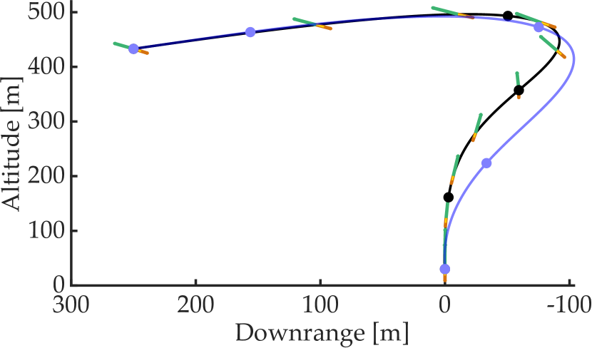
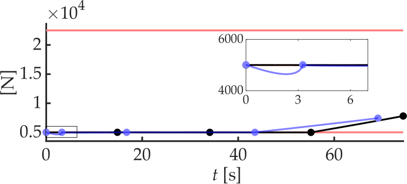
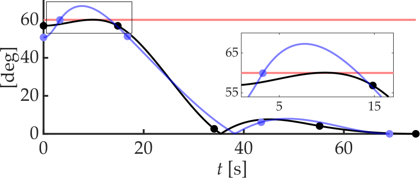
Figure 6(a) shows the position of the 6-DoF rocket along with the attitude of its body-axis (in green) and the thrust vector (as an orange-yellow plume). Figure 6(b) shows the thrust magnitude and Figure 6(c) shows the tilt of the body axis—both of which show inter-sample violation with the node-only approach.
Similar to the obstacle avoidance example, the terminal state cost with the node-only approach, kg, is smaller than that from the proposed framework, kg.
6.3 3-DoF Rocket Landing (Lossless Convexification)
This example demonstrates the application of the proposed framework for solving a convex optimal control problem. The node-only approach, in this case, amounts to solving a single convex problem where all constraints are imposed via canonical convex cones in a convex optimization solver; we use ECOS [78].
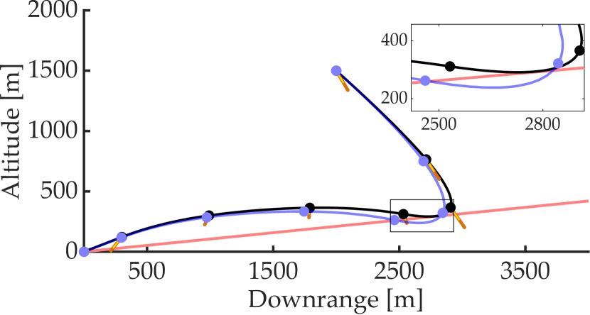
The solution from the node-only approach is used to warm-start the proposed framework, which then “cleans up” the inter-sample constraint violations. As with the previous examples, we see that the trajectory cost (in this case, fuel consumption) with the node-only approach, kg, is smaller than that from the proposed framework, kg. Figure 7(a) shows the position of the point-mass rocket along with the thrust vector (as an orange-yellow plume). The glideslope constraint shows inter-sample violation with the node-only approach. Figure 7(b) confirms that lossless convexification holds for the solutions from both methods—proposed on the left and node-only on the right. The thrust lower bound constraint shows inter-sample violation with the node-only approach, since a zero-order-hold (ZOH) parameterization is used for the mass-normalized thrust.
The node-only approach requires a dense discretization grid to ensure validity of the lossless convexification result [86], which was proven for the continuous-time problem (prior to discretization). The proposed framework, in contrast, provides a valid solution despite using a sparse discretization grid. Future work will examine whether the continuous-time lossless convexification result can apply directly to (51).
6.4 Real-Time Performance
We provide real-time performance statistics for solving the two nonconvex examples in Table 1. These results were obtained by executing pure C code generated using the sc vx gen software. The binary executables are provided in the code repository.
The mean solve-time and standard deviation (S.D.) over 1000 solves, along with the number of prox-linear iterations to convergence (Iters.), for the C implementation.
| Problem | Solve-time | S.D. | Iters. |
|---|---|---|---|
| Obstacle avoidance | ms | ms | 23 |
| 6-DoF rocket landing | ms | ms | 14 |
We note that these solve-times are on the same order-of-magnitude as the solve-times reported in the literature for real-time powered-descent guidance [87, 88, 89, 63, 90] and real-time quadrotor trajectory optimization [91, 92, 93, 94], and thus demonstrate that the proposed framework is amenable to online trajectory optimization for onboard/embedded applications.
7 Conclusions
We propose a novel trajectory optimization method that ensures continuous-time constraint satisfaction, guarantees convergence, and is real-time capable. The approach leverages an SCP algorithm called the prox-linear method along with exact penalization. When the optimal control problem is convex, we show stronger convergence property of the prox-linear method.
Future work will consider assumptions weaker than LICQ for exact penalty to hold, with the goal of developing a solution method that directly handles (24b) without relaxation, and also releasing sc vx gen, the in-house-developed code-generation software for general-purpose real-time trajectory optimization that was used to generate pure C code for the examples considered in the paper. {ack} The authors gratefully acknowledge Mehran Mesbahi, Skye Mceowen, and Govind M. Chari for helpful discussions and their feedback on the initial draft of the paper.
References
- [1] Danylo Malyuta, Yue Yu, Purnanand Elango, and Behçet Açıkmeşe. Advances in trajectory optimization for space vehicle control. Annual Reviews in Control, 52:282–315, 2021. doi:10.1016/j.arcontrol.2021.04.013.
- [2] Danylo Malyuta, Taylor P. Reynolds, Michael Szmuk, Thomas Lew, Riccardo Bonalli, Marco Pavone, and Behçet Açıkmeşe. Convex optimization for trajectory generation: A tutorial on generating dynamically feasible trajectories reliably and efficiently. IEEE Control Systems Magazine, 42(5):40–113, 2022. doi:10.1109/MCS.2022.3187542.
- [3] Panagiotis Tsiotras and Mehran Mesbahi. Toward an algorithmic control theory. Journal of Guidance, Control, and Dynamics, 40(2):194–196, 2017. doi:10.2514/1.G002754.
- [4] John T. Betts. Practical Methods for Optimal Control and Estimation Using Nonlinear Programming. Advances in Design and Control. SIAM, 2nd edition, January 2010. doi:10.1137/1.9780898718577.
- [5] John T. Betts. Survey of numerical methods for trajectory optimization. Journal of Guidance, Control, and Dynamics, 21(2):193–207, 1998. doi:10.2514/2.4231.
- [6] Anil V. Rao. A survey of numerical methods for optimal control. Advances in the Astronautical Sciences, 135(1):497–528, 2009.
- [7] Daniel Dueri, Yuanqi Mao, Zohaib Mian, Jerry Ding, and Behçet Açıkmeşe. Trajectory optimization with inter-sample obstacle avoidance via successive convexification. In 2017 IEEE 56th Conference on Decision and Control (CDC), pages 1150–1156. IEEE, December 2017. doi:10.1109/cdc.2017.8263811.
- [8] L. S. Jennings, M. E. Fisher, Kok Lay Teo, and C. J. Goh. MISER3: Solving optimal control problems–an update. Advances in Engineering Software and Workstation, 13(4):190–196, July 1991. doi:10.1016/0961-3552(91)90016-w.
- [9] Oskar von Stryk. Numerical solution of optimal control problems by direct collocation. In Optimal Control, pages 129–143. Birkhäuser Basel, 1993. doi:10.1007/978-3-0348-7539-4_10.
- [10] Victor M. Becerra. Solving complex optimal control problems at no cost with PSOPT. In 2010 IEEE International Symposium on Computer Aided Control System Design. IEEE, September 2010. doi:10.1109/cacsd.2010.5612676.
- [11] Per E. Rutquist and Marcus M. Edvall. PROPT-MATLAB optimal control software. TOMLAB Optimization, April 2010.
- [12] Michael A. Patterson and Anil V. Rao. GPOPS-II: A MATLAB software for solving multiple-phase optimal control problems using hp-adaptive gaussian quadrature collocation methods and sparse nonlinear programming. ACM Transactions on Mathematical Software, 41(1):1–37, October 2014. doi:10.1145/2558904.
- [13] Philip E. Gill, Walter Murray, and Michael A. Saunders. SNOPT: An SQP algorithm for large-scale constrained optimization. SIAM Review, August 2006. doi:10.1137/S0036144504446096.
- [14] Andreas Wächter and Lorenz T. Biegler. On the implementation of an interior-point filter line-search algorithm for large-scale nonlinear programming. Mathematical Programming, 106(1):25–57, March 2006. doi:10.1007/s10107-004-0559-y.
- [15] Richard H. Byrd, Jorge Nocedal, and Richard A. Waltz. Knitro: An integrated package for nonlinear optimization. In Nonconvex Optimization and Its Applications, pages 35–59. Springer US, 2006. doi:10.1007/0-387-30065-1_4.
- [16] Robin Verschueren, Gianluca Frison, Dimitris Kouzoupis, Jonathan Frey, Niels van Duijkeren, Andrea Zanelli, Branimir Novoselnik, Thivaharan Albin, Rien Quirynen, and Moritz Diehl. Acados-a modular open-source framework for fast embedded optimal control. Mathematical programming computation, 14(1):147–183, March 2022. doi:10.1007/s12532-021-00208-8.
- [17] Boris Houska, Hans Joachim Ferreau, and Moritz Diehl. ACADO toolkit–an open-source framework for automatic control and dynamic optimization. Optimal Control Applications and Methods, 32(3):298–312, May 2011. doi:10.1002/oca.939.
- [18] John Schulman, Yan Duan, Jonathan Ho, Alex Lee, Ibrahim Awwal, Henry Bradlow, Jia Pan, Sachin Patil, Ken Goldberg, and Pieter Abbeel. Motion planning with sequential convex optimization and convex collision checking. International Journal of Robotics Research, 33(9):1251–1270, August 2014. doi:10.1177/0278364914528132.
- [19] Lorenzo Stella, Andreas Themelis, Pantelis Sopasakis, and Panagiotis Patrinos. A simple and efficient algorithm for nonlinear model predictive control. In 2017 IEEE 56th Conference on Decision and Control (CDC), pages 1939–1944. IEEE, December 2017. doi:10.1109/cdc.2017.8263933.
- [20] Ajay Sathya, Pantelis Sopasakis, Ruben Van Parys, Andreas Themelis, Goele Pipeleers, and Panagiotis Patrinos. Embedded nonlinear model predictive control for obstacle avoidance using PANOC. In 2018 European Control Conference (ECC), pages 1523–1528, 2018. doi:10.23919/ECC.2018.8550253.
- [21] Taylor A. Howell, Kevin Tracy, Simon Le Cleac’h, and Zachary Manchester. CALIPSO: A differentiable solver for trajectory optimization with conic and complementarity constraints. In Springer Proceedings in Advanced Robotics, pages 504–521. Springer Nature Switzerland, Cham, 2023. doi:10.1007/978-3-031-25555-7\_34.
- [22] Changliu Liu, Chung-Yen Lin, and Masayoshi Tomizuka. The convex feasible set algorithm for real time optimization in motion planning. SIAM Journal of Control and Optimization, 56(4):2712–2733, January 2018. doi:10.1137/16M1091460.
- [23] Vincent Roulet, Siddhartha Srinivasa, Dmitriy Drusvyatskiy, and Zaid Harchaoui. Iterative linearized control: Stable algorithms and complexity guarantees. In Proceeding of the 36th International Conference on Machine Learning, volume 97, pages 5518–5527. PMLR, 2019. URL: https://proceedings.mlr.press/v97/roulet19a.html.
- [24] Donggun Lee, Shankar A. Deka, and Claire J. Tomlin. Convexifying state-constrained optimal control problems. IEEE Transactions on Automatic Control, pages 1–8, 2022. doi:10.1109/TAC.2022.3221704.
- [25] Xiaojing Zhang, Alexander Liniger, and Francesco Borrelli. Optimization-based collision avoidance. IEEE Transactions on Control Systems Technology, 29(3):972–983, 2021. doi:10.1109/TCST.2019.2949540.
- [26] Xinfu Liu and Ping Lu. Solving nonconvex optimal control problems by convex optimization. Journal of Guidance, Control, and Dynamics, 37(3):750–765, May 2014. doi:10.2514/1.62110.
- [27] Tobia Marcucci, Mark Petersen, David von Wrangel, and Russ Tedrake. Motion planning around obstacles with convex optimization. Science Robotics, 8(84), November 2023. doi:10.1126/scirobotics.adf7843.
- [28] Behçet Açıkmeşe, Daniel Scharf, Fred Hadaegh, and Emmanuell Murray. A convex guidance algorithm for formation reconfiguration. In AIAA Guidance Navigation and Control Conference, Reston, Virigina, August 2006. AIAA. doi:10.2514/6.2006-6070.
- [29] Behçet Açıkmeşe, Daniel Scharf, Lars Blackmore, and Aron Wolf. Enhancements on the convex programming based powered descent guidance algorithm for mars landing. In AIAA/AAS Astrodynamics Specialist Conference and Exhibit, Reston, Virigina, August 2008. AIAA. doi:10.2514/6.2008-6426.
- [30] Arthur Richards and Oliver Turnbull. Inter-sample avoidance in trajectory optimizers using mixed-integer linear programming. International Journal of Robust and Nonlinear Control, 25(4):521–526, 2015. doi:10.1002/rnc.3101.
- [31] Florian Messerer, Katrin Baumgärtner, and Moritz Diehl. Survey of sequential convex programming and generalized gauss-newton methods. ESAIM: Proceedings and Surveys, 71:64–88, August 2021. doi:10.1051/proc/202171107.
- [32] Moritz Diehl and Sebastien Gros. Numerical optimal control. https://www.syscop.de/files/2020ss/NOC/book-NOCSE.pdf. Accessed: 04-24-2024.
- [33] Rebecca Foust, Soon-Jo Chung, and Fred Y. Hadaegh. Optimal guidance and control with nonlinear dynamics using sequential convex programming. Journal of Guidance, Control, and Dynamics, 43(4):633–644, April 2020. doi:10.2514/1.g004590.
- [34] Riccardo Bonalli, Abhishek Cauligi, Andrew Bylard, and Marco Pavone. GuSTO: Guaranteed sequential trajectory optimization via sequential convex programming. In 2019 International Conference on Robotics and Automation (ICRA), pages 6741–6747, May 2019. doi:10.1109/ICRA.2019.8794205.
- [35] Riccardo Bonalli, Thomas Lew, and Marco Pavone. Analysis of theoretical and numerical properties of sequential convex programming for continuous-time optimal control. IEEE Transactions on Automatic Control, pages 1–16, 2022. doi:10.1109/TAC.2022.3207865.
- [36] Lei Xie, Xiang Zhou, Hong-Bo Zhang, and Guo-Jian Tang. Descent property in sequential second-order cone programming for nonlinear trajectory optimization. Journal of Guidance, Control, and Dynamics, pages 1–16, October 2023. doi:10.2514/1.g007494.
- [37] Lei Xie, Xiang Zhou, Hong-Bo Zhang, and Guo-Jian Tang. Higher-order soft-trust-region-based sequential convex programming. Journal of Guidance, Control, and Dynamics, pages 1–8, June 2023. doi:10.2514/1.g007266.
- [38] Quoc Tran Dinh and Moritz Diehl. Local convergence of sequential convex programming for nonconvex optimization. In Recent Advances in Optimization and its Applications in Engineering, pages 93–102. Springer Berlin Heidelberg, Berlin, Heidelberg, 2010. doi:10.1007/978-3-642-12598-0\_9.
- [39] Florian Messerer and Moritz Diehl. Determining the exact local convergence rate of sequential convex programming. In 2020 European Control Conference (ECC), pages 1280–1285. IEEE, May 2020. doi:10.23919/ecc51009.2020.9143749.
- [40] Adrian Lewis and Stephen Wright. A proximal method for composite minimization. Mathematical Programming, 158(1-2):501–546, July 2016. doi:10.1007/s10107-015-0943-9.
- [41] Coralia Cartis, Nicholas I. M. Gould, and Philippe L. Toint. On the evaluation complexity of composite function minimization with applications to nonconvex nonlinear programming. SIAM Journal on Optimization, 21(4):1721–1739, October 2011. doi:10.1137/11082381X.
- [42] Dmitriy Drusvyatskiy and Adrian Lewis. Error bounds, quadratic growth, and linear convergence of proximal methods. Mathematics of Operations Research, 43(3):919–948, 2018. doi:10.1287/moor.2017.0889.
- [43] Zhenbo Wang and Michael J. Grant. Constrained trajectory optimization for planetary entry via sequential convex programming. Journal of Guidance, Control, and Dynamics, 40(10):2603–2615, October 2017. URL: http://doi.org/10.2514/1.G002150, doi:10.2514/1.g002150.
- [44] Michael Szmuk, Taylor P. Reynolds, and Behçet Açıkmeşe. Successive convexification for real-time six-degree-of-freedom powered descent guidance with state-triggered constraints. Journal of Guidance, Control, and Dynamics, 43(8):1399–1413, August 2020. doi:10.2514/1.G004549.
- [45] Marco Sagliano. Pseudospectral convex optimization for powered descent and landing. Journal of Guidance, Control, and Dynamics, 41(2):320–334, February 2018. URL: http://doi.org/10.2514/1.G002818, doi:10.2514/1.g002818.
- [46] Hans Georg Bock and Karl-Josef Plitt. A multiple shooting algorithm for direct solution of optimal control problems. IFAC Proceedings Volumes, 17(2):1603–1608, 1984. doi:10.1016/S1474-6670(17)61205-9.
- [47] Robert McGill. Optimum control, inequality state constraints, and the generalized newton-raphson algorithm. Journal of the Society for Industrial and Applied Mathematics, 3(2):291–298, January 1965. doi:10.1137/0303021.
- [48] R. W. H. Sargent and G. R. Sullivan. The development of an efficient optimal control package. In Proceedings of the 8th IFIP Conference on Optimization Techniques, Würzburg, September 5–9, 1977, volume 7, pages 158–168, Berlin/Heidelberg, 1977. Springer-Verlag. doi:10.1007/bfb0006520.
- [49] Kok Lay Teo and C Goh. A simple computational procedure for optimization problems with functional inequality constraints. IEEE Transactions on Automatic Control, 32(10):940–941, October 1987. doi:10.1109/tac.1987.1104471.
- [50] R C Loxton, K L Teo, V Rehbock, and K F C Yiu. Optimal control problems with a continuous inequality constraint on the state and the control. Automatica, 45(10):2250–2257, October 2009. doi:10.1016/j.automatica.2009.05.029.
- [51] Qun Lin, Ryan Loxton, Kok Lay Teo, Yong Hong Wu, and Changjun Yu. A new exact penalty method for semi-infinite programming problems. Journal of Computational and Applied Mathematics, 261:271–286, May 2014. doi:10.1016/j.cam.2013.11.010.
- [52] Dmitriy Drusvyatskiy and Courtney Paquette. Efficiency of minimizing compositions of convex functions and smooth maps. Mathematical Programming, 178:503–558, 2019. doi:10.1007/s10107-018-1311-3.
- [53] Govind M. Chari, Abhinav G. Kamath, Purnanand Elango, and Behçet Açıkmeşe. Fast monte carlo analysis for 6-DoF powered-descent guidance via GPU-accelerated sequential convex programming. In AIAA SciTech 2024 Forum. AIAA, January 2024. doi:10.2514/6.2024-1762.
- [54] Samet Uzun, Purnanand Elango, Abhinav G. Kamath, Taewan Kim, and Behçet Açıkmeşe. Successive convexification for nonlinear model predictive control with continuous-time constraint satisfaction. In 8th IFAC Conference on Nonlinear Model Predictive Control, Kyoto, Japan, August 2024.
- [55] Taewan Kim, Niyousha Rahimi, Abhinav G. Kamath, Jasper Corleis, Behçet Açıkmeşe, and Mehran Mesbahi. Approach and landing trajectory optimization for a 6-DoF aircraft with a runway alignment constraint, 2024.
- [56] Stephen Boyd and Lieven Vandenberghe. Convex Optimization. Cambridge University Press, March 2004. doi:10.1017/CBO9780511804441.
- [57] Jean-Baptiste Hiriart-Urruty and Claude Lemarechal. Convex Analysis and Minimization Algorithms I: Fundametals. Grundlehren der mathematischen Wissenschaften. Springer, Berlin, Germany, 1993. doi:10.1007/978-3-662-02796-7.
- [58] Daniel Liberzon. Calculus of Variations and Optimal Control Theory: A Concise Introduction. Princeton University Press, December 2011.
- [59] Leonard D. Berkovitz. Optimal Control Theory. Applied Mathematical Sciences. Springer, New York, NY, February 1974. doi:10.1007/978-1-4757-6097-2.
- [60] Francis H. Clarke, Yuri S. Ledyaev, Ronald J. Stern, and Peter R. Wolenski. Nonsmooth Analysis and Control Theory, volume 178 of Graduate Texts in Mathematics. Springer Verlag, New York, 1998. doi:10.1007/b97650.
- [61] Gerald B. Folland. Real Analysis: Modern Techniques and their Applications, volume 40. John Wiley & Sons, 1999.
- [62] R. Quirynen, M. Vukov, M. Zanon, and M. Diehl. Autogenerating microsecond solvers for nonlinear MPC: A tutorial using ACADO integrators. Optimal Control Applications and Methods, 36(5):685–704, September 2015. doi:10.1002/oca.2152.
- [63] Abhinav G. Kamath, Purnanand Elango, Yue Yu, Skye Mceowen, Govind M. Chari, John M. Carson, III, and Behçet Açıkmeşe. Real-time sequential conic optimization for multi-phase rocket landing guidance. IFAC-PapersOnLine, 56(2):3118–3125, 2023. doi:10.1016/j.ifacol.2023.10.1444.
- [64] H. W. J. Lee, Kok Lay Teo, V. Rehbock, and L. S. Jennings. Control parametrization enhancing technique for time optimal control problems. Dynamic Systems and Applications, pages 243–261, 1997.
- [65] Qun Lin, Ryan Loxton, and Kok Lay Teo. The control parameterization method for nonlinear optimal control: A survey. Journal of Industrial and Management Optimization, 10(1):275–309, 2014. doi:10.3934/jimo.2014.10.275.
- [66] Divya Garg, Michael Patterson, William W. Hager, Anil V. Rao, David A. Benson, and Geoffrey T. Huntington. A unified framework for the numerical solution of optimal control problems using pseudospectral methods. Automatica, 46(11):1843–1851, 2010. doi:10.1016/j.automatica.2010.06.048.
- [67] I. Michael Ross and Mark Karpenko. A review of pseudospectral optimal control: From theory to flight. Annual Reviews in Control, 36(2):182–197, December 2012. doi:10.1016/j.arcontrol.2012.09.002.
- [68] Runqi Chai, Kaiyuan Chen, Lingguo Cui, Senchun Chai, Gokhan Inalhan, and Antonios Tsourdos. Advanced Trajectory Optimization, Guidance and Control Strategies for Aerospace Vehicles: Methods and Applications. Springer Nature Singapore, Singapore, 2023. doi:10.1007/978-981-99-4311-1.
- [69] Jorge Nocedal and Stephen Wright. Numerical Optimization. Springer, 2nd edition, July 2006. doi:10.1007/978-0-387-40065-5.
- [70] Danylo Malyuta, Taylor P. Reynolds, Michael Szmuk, Mehran Mesbahi, Behçet Açıkmeşe, and John M. Carson III. Discretization performance and accuracy analysis for the rocket powered descent guidance problem. In AIAA SciTech 2019 Forum, Reston, Virginia, January 2019. doi:10.2514/6.2019-0925.
- [71] Ricard Bordalba, Tobias Schoels, Lluis Ros, Josep M. Porta, and Moritz Diehl. Direct collocation methods for trajectory optimization in constrained robotic systems. IEEE Transactions on Robotics, pages 1–20, 2022. doi:10.1109/TRO.2022.3193776.
- [72] Jun Fu, Johannes M. M. Faust, Benoît Chachuat, and Alexander Mitsos. Local optimization of dynamic programs with guaranteed satisfaction of path constraints. Automatica, 62:184–192, December 2015. doi:10.1016/j.automatica.2015.09.013.
- [73] Fernando A. C. C. Fontes and Luis Tiago Paiva. Guaranteed constraint satisfaction in continuous-time control problems. IEEE Control Systems Letters, 3(1):13–18, 2019. doi:10.1109/LCSYS.2018.2849853.
- [74] Jun Fu and Fangyin Tian. Dynamic optimization of nonlinear systems with guaranteed feasibility of inequality-path-constraints. Automatica, 127(109516):109516, May 2021. doi:10.1016/j.automatica.2021.109516.
- [75] S. P. Han and Olvi L. Mangasarian. Exact penalty functions in nonlinear programming. Mathematical Programming, 17:251–269, 1979. doi:10.1007/BF01588250.
- [76] G. Di Pillo and L. Grippo. On the exactness of a class of nondifferentiable penalty functions. Journal of Optimization Theory and Applications, 57(3):399–410, 1988. doi:10.1007/BF02346160.
- [77] G. Di Pillo and L. Grippo. Exact penalty functions in constrained optimization. SIAM Journal of Control and Optimization, 27(6):1333–1360, 1989. doi:10.1137/0327068.
- [78] Alexander Domahidi, Eric Chu, and Stephen Boyd. ECOS: An SOCP solver for embedded systems. In 2013 European Control Conference (ECC), pages 3071–3076, July 2013. doi:10.23919/ECC.2013.6669541.
- [79] MOSEK ApS. The MOSEK optimization toolbox for MATLAB manual. Version 10.1., 2024. URL: http://docs.mosek.com/latest/toolbox/index.html.
- [80] Francis Clarke. Functional Analysis, Calculus of Variations and Optimal Control, volume 264. Springer, 2013. doi:10.1007/978-1-4471-4820-3.
- [81] Amir Beck. First-Order Methods in Optimization. SIAM, 2017. doi:10.1137/1.9781611974997.
- [82] Yue Yu, Purnanand Elango, Behçet Açıkmeşe, and Ufuk Topcu. Extrapolated proportional-integral projected gradient method for conic optimization. IEEE Control Systems Letters, 7:73–78, 2022. doi:10.1109/LCSYS.2022.3186647.
- [83] Taylor P. Reynolds and Mehran Mesbahi. The crawling phenomenon in sequential convex programming. In 2020 American Control Conference (ACC), pages 3613–3618, July 2020. doi:10.23919/ACC45564.2020.9147550.
- [84] Taylor P. Reynolds, Michael Szmuk, Danylo Malyuta, Mehran Mesbahi, Behçet Açıkmeşe, and John M. Carson III. Dual quaternion-based powered descent guidance with state-triggered constraints. Journal of Guidance, Control, and Dynamics, 43(9):1584–1599, September 2020. doi:10.2514/1.G004536.
- [85] Michael Garstka, Mark Cannon, and Paul Goulart. COSMO: A conic operator splitting method for convex conic problems. Journal of Optimization Theory and Applications, 190(3):779–810, September 2021. doi:10.1007/s10957-021-01896-x.
- [86] Behçet Açıkmeşe, John M. Carson III, and Lars Blackmore. Lossless convexification of nonconvex control bound and pointing constraints of the soft landing optimal control problem. IEEE Transactions on Control Systems Technology, 21(6):2104–2113, November 2013. doi:10.1109/tcst.2012.2237346.
- [87] Daniel Dueri, Behçet Açıkmeşe, Daniel P. Scharf, and Matthew W. Harris. Customized real-time interior-point methods for onboard powered-descent guidance. Journal of Guidance, Control, and Dynamics, 40(2):197–212, February 2017. doi:10.2514/1.g001480.
- [88] Taylor Reynolds, Danylo Malyuta, Mehran Mesbahi, Behçet Açıkmeşe, and John M. Carson III. A real-time algorithm for non-convex powered descent guidance. In AIAA SciTech 2020 Forum. AIAA, January 2020. doi:10.2514/6.2020-0844.
- [89] Purnanand Elango, Abhinav G. Kamath, Yue Yu, John M. Carson III, Mehran Mesbahi, and Behçet Açıkmeşe. A customized first-order solver for real-time powered-descent guidance. In AIAA SciTech 2022 Forum. AIAA, January 2022. doi:10.2514/6.2022-0951.
- [90] Abhinav G. Kamath, Purnanand Elango, Taewan Kim, Skye Mceowen, Yue Yu, John M. Carson III, Mehran Mesbahi, and Behçet Açıkmeşe. Customized real-time first-order methods for onboard dual quaternion-based 6-DoF powered-descent guidance. In AIAA SciTech 2023 Forum. AIAA, January 2023. doi:10.2514/6.2023-2003.
- [91] Michael Szmuk, Carlo Alberto Pascucci, Daniel Dueri, and Behçet Açıkmeşe. Convexification and real-time on-board optimization for agile quad-rotor maneuvering and obstacle avoidance. In 2017 IEEE/RSJ International Conference on Intelligent Robots and Systems (IROS). IEEE, September 2017. doi:10.1109/iros.2017.8206363.
- [92] Michael Szmuk, Carlo Alberto Pascucci, and Behçet acikmese. Real-time quad-rotor path planning for mobile obstacle avoidance using convex optimization. In 2018 IEEE/RSJ International Conference on Intelligent Robots and Systems (IROS). IEEE, October 2018. doi:10.1109/iros.2018.8594351.
- [93] Michael Szmuk, Danylo Malyuta, Taylor P. Reynolds, Margaret Skye Mceowen, and Behçet Açıkmeşe. Real-time quad-rotor path planning using convex optimization and compound state-triggered constraints. In 2019 IEEE/RSJ International Conference on Intelligent Robots and Systems (IROS). IEEE, November 2019. doi:10.1109/iros40897.2019.8967706.
- [94] Yue Yu, Kartik Nagpal, Skye Mceowen, Behçet Açıkmeşe, and Ufuk Topcu. Real-time quadrotor trajectory optimization with time-triggered corridor constraints. Journal of Guidance, Control, and Dynamics, 46(6):1197–1205, June 2023. doi:10.2514/1.g007218.
- [95] Philip J. Davis. Interpolation and Approximation. Dover Publications, 1975.
- [96] MOSEK Cookbook 3.3.0. https://docs.mosek.com/modeling-cookbook/index.html. Accessed: 03-26-2024.
- [97] Behçet Açıkmeşe and Scott R. Ploen. Convex programming approach to powered descent guidance for mars landing. Journal of Guidance, Control, and Dynamics, 30(5):1353–1366, 2007. doi:10.2514/1.27553.
Appendix
Appendix A Proof of Theorem 14
As a consequence of the relaxation in (26c), we wish to bound and on the interval , for any and .
Lemma 31.
Time derivative of path constraint functions and are bounded almost everywhere on the state trajectory and control input .
Proof: Note that the augmented control input parameterization (20) is a piecewise polynomial, which is differentiable almost everywhere in . Then, due to (26d) and Remark 13, and are bounded for , , and is well-defined and bounded . The state trajectory is bounded due to Assumption 1. Further, , for , is bounded. Consequently, , , and are bounded, where , , and . Then, through the chain-rule
| (59) |
with , we infer that and are bounded almost everywhere.
We denote the upper bounds on the absolute values of and (which hold almost everywhere) with and , respectively.
When (26c) and the penultimate row of (26b) are satisfied, for any , we have that
for any and , where we use the change of variable , for .
First, we examine the pointwise bound on . We denote compactly with , and let denote the maximum absolute value of within the interval . We assume, without loss of generality, that is attained at . Next, we approximate the area under , for , via an auxiliary function given by
Note that, for , we have
Therefore, is positive for and . If , we have that , where . The area under , for , is triangular (Figure 8(a)). Then,
| (60a) | |||
| (60b) | |||
| (60c) | |||
Conversely, if , we have that . The area under within is trapezoidal (Figure 8(b)). Then,
| (61a) | |||
| (61b) | |||
| (61c) | |||
| (61d) | |||
where is the lower bound for ; it exists because the dilation factor is positive and , for . Note that holds only if
This case can be ignored in practice since we are interested in small which is physically insignificant. Hence, from (60c), we have
| (62) |
for . We can similarly bound the maximum value of , denoted by , by approximating the area under , for , to obtain
| (63) |
for .
Appendix B Control Input Parameterization
B.1 First-Order-Hold
Choose and define
In other words,
| (65) |
whenever for some . Note that is the Kronecker delta, for . As a result, , for .
B.2 Pseudospectral Methods
In pseudospectral methods, the control input is parameterized with a basis of orthogonal polynomials, i.e.,
| (66) |
is the Lagrange interpolating polynomial [95, Sec. 2.5] of degree , where , for , are related to the roots of orthogonal polynomials (such as members of the Jacobi family [95, Sec. 10.3]). For e.g., choosing to be the roots of the polynomial
| (67) |
would correspond to Chebyshev-Gauss-Lobatto (CGL) collocation [70, Sec. D.1], where defined by is the Chebyshev polynomial of degree [95, Def. 3.3.1]. The choice of basis functions (66) ensures that , for each . As a result, , for .
Appendix C Dynamic Obstacle Avoidance
We consider a two-dimensional free-final-time path planning problem. The dynamical system describing the vehicle comprises of position , velocity , cumulative cost , and acceleration input . The state , augmented state , and augmented control input are given by
| (68a) | ||||
| (68b) | ||||
| (68c) | ||||
We choose a first-order-hold (see Appendix B.1) parameterization for the augmented control input.
The augmented system is given by
| (74) |
where is the drag coefficient. The vehicle is subject to the following inequality path constraints: avoidance of moving elliptical obstacles, speed upper bound, and acceleration upper- and lower bounds, which are encoded in the path constraint function as follows
| (81) |
The shape matrix and center of the th obstacle at time are and , respectively, for . A sinusoidal motion is prescribed for the centers of the obstacles, i.e.,
| (82) |
with amplitude , phase angle , and frequency , about the nominal center . The speed upper bound and the acceleration upper- and lower bounds are , , and , respectively. The boundary conditions are specified through function as follows
| (83) |
where and are the initial position and velocity, respectively, and and are the final position and velocity, respectively. We set the terminal state cost function to . Constraint functions and are not utilized in this example.
Table 2 shows the parameter values chosen for the system and the algorithm to generate the results in Section 6.1. In addition, we choose the following parameter values for the sinusoidal motion given by (82)
where is the th column of , for . The scenario with static obstacles in Section 6.1 is generated by setting .
| Parameter | Value |
|---|---|
| m-1 | |
| , | , m |
| , | , m s-1 |
| m s-1 | |
| , | , m s-2 |
| , | |
| s | |
| , | |
Appendix D 6-DoF Rocket Landing
We consider a free-final-time 6-DoF lunar landing scenario based on the formulation given in [44], and adopt the notation therein. The state , control input , augmented state , and augmented control input are given by
| (84a) | ||||
| (84b) | ||||
| (84c) | ||||
| (84d) | ||||
We choose a first-order-hold (see Appendix B.1) parameterization for the augmented control input.
The augmented dynamical system is given by
| (85) |
The path constraint function is given by
| (86) |
where the second-order-cone constraints on and are equivalently reformulated to quadratic forms to ensure continuous differentiability [96, Sec. 3.2.4]. The boundary conditions are specified through function as follows
| (87) |
where and are the initial position and velocity, respectively, and are the final position and velocity, respectively, and is the unit quaternion. The terminal state cost function is set to . Constraint functions and are not utilized in this example.
Table 3 shows the parameter values chosen for the system and the algorithm to generate the results in Section 6.2. The definitions of and are taken from [44].
| Parameter | Value |
|---|---|
| s m-1 | |
| m s-2 | |
| m | |
| kg m2 | |
| , | , kg |
| , | , m |
| , | , m s-1 |
| m s-1 | |
| s-1 | |
| s | |
| , | , N |
| , | , |
Appendix E 3-DoF Rocket Landing
We consider a convex, fixed-final-time Mars landing scenario based on the dynamical system and constraints in [97, 89]. The state and control input are given by
| (88) | ||||
| (89) |
where is the vehicle mass, is the thrust vector, and is an auxiliary control input (slack variable) introduced as a part of the lossless convexification procedure. We choose a zero-order-hold parameterization for the control input.
We consider the following linear dynamical system
| (90) | ||||
The path constraint function is given by
| (91) | |||
where , , and
| (92a) | ||||
| (92b) | ||||
| (92c) | ||||
| (92d) | ||||
Lossless convexification holds if . The boundary conditions are specified through function as follows
| (93) |
where and are the initial position and velocity, respectively, and and are the final position and velocity, respectively. The terminal state cost function is set to . The running cost function , and constraint functions and , are not utilized in this example.
Table 4 shows the parameter values chosen for the system and the algorithm to generate the results in Section 6.3.
| Parameter | Value |
|---|---|
| s m-1 | |
| m s-2 | |
| , | , m |
| , | , m s-1 |
| , | , kg |
| 139 m s-1 | |
| , | , N |
| s | |