In-Context Freeze-Thaw Bayesian Optimization
for Hyperparameter Optimization

Abstract

With the increasing computational costs associated with deep learning, automated hyperparameter optimization methods, strongly relying on black-box Bayesian optimization (BO), face limitations. Freeze-thaw BO offers a promising grey-box alternative, strategically allocating scarce resources incrementally to different configurations. However, the frequent surrogate model updates inherent to this approach pose challenges for existing methods, requiring retraining or fine-tuning their neural network surrogates online, introducing overhead, instability, and hyper-hyperparameters. In this work, we propose FT-PFN, a novel surrogate for Freeze-thaw style BO. FT-PFN is a prior-data fitted network (PFN) that leverages the transformers’ in-context learning ability to efficiently and reliably do Bayesian learning curve extrapolation in a single forward pass. Our empirical analysis across three benchmark suites shows that the predictions made by FT-PFN are more accurate and 10-100 times faster than those of the deep Gaussian process and deep ensemble surrogates used in previous work. Furthermore, we show that, when combined with our novel acquisition mechanism (MFPI-random), the resulting in-context freeze-thaw BO method (ifBO), yields new state-of-the-art performance in the same three families of deep learning HPO benchmarks considered in prior work.

1 Introduction

Hyperparameters are essential in deep learning (DL) to achieve strong model performance. However, due to the increasing complexity of these models, it is becoming more challenging to find promising hyperparameter settings, even with the help of hyperparameter optimization (HPO, Section 3.1) tools (Feurer & Hutter, 2019; Bischl et al., 2023). Traditional HPO techniques using Bayesian Optimization (BO) are unsuitable for modern DL because they treat the problem as a black box, making it computationally expensive requiring a full model training for each evaluation.

Recent research in HPO has shifted towards multi-fidelity methods (Li et al., 2017, 2020a; Falkner et al., 2018; Klein et al., 2020; Li et al., 2020b; Awad et al., 2021), utilizing lower fidelity proxies (e.g., training for fewer steps, using less data, smaller models) and only evaluating the most promising hyperparameter settings at the full fidelity. While these methods have potential, they often use coarse-grained fidelity spaces and rely on the rank correlation of performances across fidelities. Moreover, they do not fully utilize the anytime nature of algorithms such as checkpointing, continuation, and extrapolation. As a result, these methods struggle to allocate computational resources efficiently, leading to suboptimal performance in many scenarios.

The freeze-thaw BO method (FT-BO, Section 3.2), originally proposed by Swersky et al. (2014), is a promising approach to efficiently allocate computational resources by pausing and resuming the evaluation of different hyperparameter configurations. This method is an improvement over traditional grey-box methods as it dynamically manages resources, and recent implementations (Wistuba et al., 2022; Kadra et al., 2023) hold the state-of-the-art in the low-budget regime ($\sim$ 20 full function evaluations). However, these contemporary implementations have limitations. In particular, they rely on online learning to update the surrogate model at each step which can lead high computational overhead, instability, and complexity in managing additional hyper-hyperparameters. Moreover, they also suffer from strong assumptions about learning curves, which may not be applicable in all scenarios, resulting in overly confident incorrect predictions.

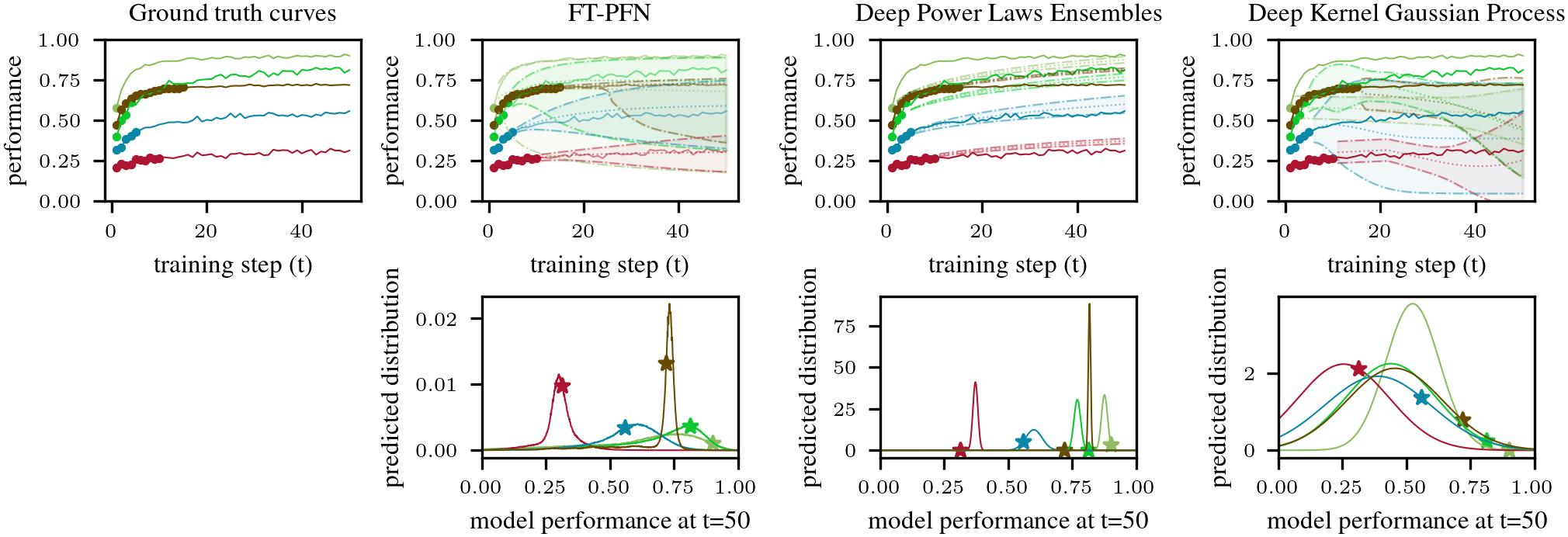
Figure 1: Comparison of prediction at a horizon of $50$ steps, given the same set of hyperparameters and their learning curves. The Ground truth curves show the real learning curves with dots ($\mathop{\mathchoice{\vbox{\hbox{\LARGE$\cdot$}}}{\vbox{\hbox{\LARGE$\cdot$}}}{\vbox{\hbox{\normalsize$\cdot$}}}{\vbox{\hbox{\small$\cdot$}}}}$) indicating the points observed as training set or context for all the surrogates. ifBO uses FT-PFN as its surrogate, which requires no refitting but instead uses the training dots as context for inferring the posterior predictive distribution at step $50$ for the given hyperparameters. DPL and DyHPO, use Deep Power Laws Ensembles and Deep Kernel Gaussian Process respectively, are trained on the training set till convergence and then used to extrapolate the given HPs. The bottom row plots the log-likelihood of the prediction of each HP at step $50$, with the stars ($\star$) indicating the true value of the curve.

In this work, we leverage prior-data fitted networks (Müller et al., 2022, PFNs) (Section 3.3), a Transformer-based meta-learning approach to Bayesian inference, to enhance freeze-thaw BO through in-context learning. Our PFN model (FT-PFN) infers the task-specific relationship between hyperparameter settings and their learning curves in a single forward pass, eliminating the need for online training during the search. Figure 1 compares learning curves extrapolation, including uncertainty, by our model (FT-PFN) and two baselines. Beyond demonstrating superior extrapolation quality, our model directly addresses key challenges in traditional HPO methods, lowering computational overhead and stabilizing the optimization process. The contributions of this paper are as follows.

• We propose FT-PFN (Section 4.1), a new surrogate model for freeze-thaw BO, replacing online learning with in-context learning using PFNs. We train a single instance of FT-PFN model exclusively on synthetic data, generated from a curve prior (Section 4.1) designed to mimic realistic HPO learning curves.

• We empirically show that FT-PFN outperforms existing surrogates, at point prediction and posterior distribution approximation, while being over an order of magnitude faster, and despite never having been trained on real HPO data (Section 5.1).

• We combine FT-PFN with a novel acquisition function (MFPI-random, Section 4.2) and find that the resulting in-context freeze-thaw method (ifBO) yields a new state-of-the-art performance on the three benchmark suites for HPO for deep learning (LCBench, Taskset, PD1).

We will publicly release the code for the surrogate PFN training and reproducing experiments from this paper.

2 Related Work

Multi-fidelity hyperparameter optimization

uses low-cost approximations of the objective function, for example, by evaluating only a few epochs of model training. A notable approach in this category is Hyperband (Li et al., 2017), which iteratively allocates a similar budget to various candidate hyperparameter settings and retains only the most promising ones, to be evaluated at a higher budget. Hyperband was extended for efficient parallelization (Li et al., 2020a), Bayesian optimization (Falkner et al., 2018) and evolutionary search (Awad et al., 2021) and to incorporate user priors (Mallik et al., 2023). However, a key limitation of these multi-fidelity approaches is that they do not allow the continuation of previously discarded runs in the light of new evidence, resulting in a waste of computational resources. Additionally, their effectiveness heavily depends on a good manual choice of fidelity levels and a strong correlation between the ranks of hyperparameter settings at low and high fidelities (e.g., no crossings of learning curves).

A promising research direction to mitigate these limitations involves predicting performance at higher fidelities. Domhan et al. (2015) addressed this by proposing a Bayesian learning curve extrapolation (LCE) method. Then, Klein et al. (2017) extended the latter approach to jointly model learning curves and hyperparameter values with Bayesian Neural Networks. Non-Bayesian versions of LCE have also been explored by Chandrashekaran & Lane (2017) and  Gargiani et al. (2019). Despite the robust extrapolation capabilities of these LCE methods, fully leveraging them in guiding HPO remains a challenge.

Freeze-Thaw Bayesian Optimization

offers a promising solution to address the limitations of standard multi-fidelity and LCE-based HPO. Its ability to pause and resume optimization runs enables the efficient management of computational resources and ensures solid anytime performance. As a BO method, it incorporates a surrogate model to predict performance at higher fidelities and relies on the acquisition function to guide the search. The freeze-thaw concept was introduced by Swersky et al. (2014), who used an entropy search acquisition function and a Gaussian Process with exponential decay kernel for modeling learning curves. Wistuba et al. (2022) recently proposed DyHPO, an improved version that uses a learned deep kernel combined with a multi-fidelity-based Expected Improvement (EI) acquisition. Most recently, Kadra et al. (2023) introduced DPL, another surrogate model that utilizes a deep ensemble of power laws and Expected Improvement at the maximum budget as acquisition function. These Freeze-Thaw BO methods substantially improve upon standard multi-fidelity approaches, showing particularly strong performance in low-budget settings. Nevertheless, these methods share a common challenge: the necessity for online training of a surrogate model during the search, which can be computationally intensive and may cause optimization instabilities.

In-context Learning (ICL)

is an exciting new learning paradigm that offers a promising alternative to online learning methods. A key advantage of ICL is that it does not require retraining / fine-tuning the model with new data, but instead, the data is fed to the model as a contextual prompt. ICL first gained a lot of interest with the rise of Transformer-based models like Large Language Models (Radford et al., 2019, LLMs) and has since also been explored as an end-to-end approach to black box HPO (Chen et al., 2022).

Prior data fitted networks,

proposed by Müller et al. (2022), are transformer-based models that are trained to do in-context Bayesian prediction. They have been successfully used as an in-context classifier for tabular data (Hollmann et al., 2023), an in-context surrogate model for black-box HPO (Müller et al., 2023), an in-context model for Bayesian learning curve extrapolation (Adriaensen et al., 2023), and an in-context time-series forecaster (Dooley et al., 2023). Our approach draws on and expands these prior works to create an efficient in-context surrogate model for freeze-thaw BO.

3 Preliminaries

We now discuss some preliminaries that we build on more formally, introducing our notation along the way.

3.1 Hyperparameter Optimization (HPO)

Consider an iterative machine training pipeline with configurable hyperparameters $\lambda\in\Lambda$. E.g., when training a neural network using gradient descent we could configure the learning rate, weight decay, dropout rate, etc. Let $f(\lambda,t)$ be some measure of downstream performance (e.g., validation loss) of the model obtained, using hyperparameter settings $\lambda$, after $t$ iterations of training, that we would like to minimize. Further, assume that the training run for any $\lambda$ is limited to $b_{\text{max}}$ such iterations. HPO aims to find a hyperparameter setting producing the best model, i.e., $\lambda^{*}$: $(\lambda^{*},\cdot)\in\operatorname*{arg\!min}_{\lambda\in\Lambda,t\in\mathbb{N}_{0}}f(\lambda,t)$, within the limited total optimization budget of $B$ iterations. Note that in modern deep learning the budget available for HPO often does not allow us to execute more than a few full training runs. In this setting, the crux of HPO lies in allocating these limited training resources to the most promising hyperparameter settings, i.e., to find an allocation $\{b_{\lambda}\}_{\lambda\in\Lambda}$ with $\sum_{\lambda\in\Lambda}b_{\lambda}=B$ that minimizes $\min_{\lambda\in\Lambda,\,1\leq t\leq b_{\lambda}}f(\lambda,t)$.

3.2 Freeze-Thaw Bayesian Optimization (FT-BO)

As discussed above, Swersky et al. (2014) proposed to address this challenge by following a fine-grained dynamic scheduling approach, allocating resources to configurations (and observing their performance) “one step at a time”. Here, one “step”, denoted as $\mathds{1}_{b}$, corresponds to one or more iterations of model training (e.g., one epoch). Algorithm 1 shows the freeze-thaw Bayesian optimization framework (FT-BO) which uses its history $H$, i.e., the various partial learning curves observed thus far in the current partial allocation, to fit a dynamic Bayesian surrogate model $\mathcal{M}{}$ that probabilistically extrapolates the partially seen performance of configuration $\lambda$ beyond $b_{\lambda}$ (Algorithm 1, line 4). Following the BO framework, it decides which of these to continue (or start if $b_{\lambda}=0$) using a dynamic acquisition policy $\mathcal{A}{}$ trading off exploration and exploitation (Algorithm 1, line 5). The crucial difference with traditional black box Bayesian Optimization lies in that resources in FT-BO are allocated one step, rather than one full training run, at the time. Note, FT-BO assumes training to be preemptive, i.e., that we can stop (freeze) a model training, and continue (thaw) it later; this assumption is reasonable in modern DL where checkpointing is common practice. Also note, that black box BO can be recovered as a special case, by setting $b_{\text{max}}$, the maximum number of steps allocated to any single configuration, to one, and $\mathds{1}_{b}$ to the maximum budget available for any single training run.

Algorithm 1 Freeze-thaw Bayesian Optimization. Blue comments detail ifBO specifics.

Input: $\Lambda$: configuration space,
         $f$: measure of model performance to be minimized,
         $\mathds{1}_{b}$: iterations of model training per freeze-thaw step,
         $b_{\text{max}}$: maximal steps for any configuration $\lambda\in\Lambda$,
         $B$: total HPO budget in iterations of model training.
Components:
   $\mathcal{M}{}$: the dynamic surrogate model (FT-PFN),
   $\mathcal{A}{}$: the dynamic acquisition policy (MFPI-random, Alg. 2)
Output: $\lambda\in\Lambda$, that obtained the best performance observed

Procedure: HPO($\Lambda$, $f$, $\mathds{1}_{b}$, $b_{\text{max}}$, $B$):

1:  $\lambda\sim\mathcal{U}(\Lambda)\lx@algorithmic@hfill$ initial random sample

2:  $H\leftarrow{}\{(\lambda,{\color[rgb]{0,0,0}1},f(\lambda,\mathds{1}_{b}))\}\lx@algorithmic@hfill$ evaluate $f$ (train $\lambda$ for one step)

2:  

3:  while $|H|\cdot\mathds{1}_{b}<B$ do

4:     Train $\mathcal{M}{}$ on $H$ FT-PFN requires no model fitting

5:     $\lambda\xleftarrow{}$ $\mathcal{A}{}$($\Lambda,\mathcal{M}{},H,b_{\text{max}}$) select $\lambda$ to thaw

6:     ${\color[rgb]{0,0,0}n_{\lambda}\leftarrow{}\max\{z\}_{(\lambda,z,y)\in H}}$$n_{\lambda}$: steps performed using $\lambda$

7:     $y\leftarrow{}f(\lambda,(n_{\lambda}+1)$$\cdot\mathds{1}_{b})$evaluate $f$ (thaw $\lambda$ for one step)

8:     $H\leftarrow H\cup\{(\lambda,n_{\lambda}+1,y)\}$

9:  end while

9:  

10:  return $\lambda^{*}$: $(\lambda^{*},\cdot)\in\operatorname*{arg\!min}_{\lambda\in\Lambda,\,1\leq z\leq n_{\lambda}}f(\lambda,z\cdot\mathds{1}_{b})$

3.3 Prior-data Fitted Networks (PFNs)

As briefly discussed above, PFNs (Müller et al., 2022) are neural networks $q_{\theta}$ that are trained to do Bayesian prediction for supervised learning in a single forward pass. More specifically, let $D=D_{train}\cup\{(x_{test},y_{test})\}$ be a dataset used for training; the PFN’s parameters $\theta$ are optimized to take $D_{train}$ and $x_{test}$ as inputs and make predictions that approximate the posterior predictive distribution (PPD) of the output label $y_{test}$:

$$q_{\theta}(x_{test},D_{train})\approx\mathbb{P}(y_{test}\,|\,x_{test},D_{train}),$$

in expectation over datasets $D$ sampled from a prior $p(\mathcal{D})$ over datasets. At test time, the PFN does not update its parameters by gradient descent given a training dataset $D_{train}$, but rather takes $D_{train}$ as a contextual input, predicting the labels of unseen examples through in-context learning. The PFN is pretrained once for a specific prior $p(\mathcal{D})$ and used in downstream Bayesian prediction tasks without further fine-tuning. More specifically, it is trained to minimize the cross-entropy for predicting the hold-out example's label $y_{test}$, given $x_{test}$ and $D_{train}$:

$$\begin{split}\ell_{\theta}=\mathbb{E}[\shortminus\text{log}\ q_{\theta}(y_{test}|x_{test},D_{train})]\\ \text{with \quad}\{(x_{test},y_{test})\}\cup D_{train}\sim p(\mathcal{D})\end{split}$$ (1)

Müller et al. (2022) proved that this training procedure coincides with minimizing the KL divergence between the PFN's predictions and the true PPD.

4 In-Context Freeze-Thaw BO (ifBO)

In this section, we describe ifBO, the in-context learned variant of the freeze-thaw framework that we propose as an alternative for the existing online learning implementations (Wistuba et al., 2022; Kadra et al., 2023). As can be seen in Algorithm 1 (line 4), the critical difference lies in the fact that we do not need to refit our surrogate model after every allocation step, but instead provide the full history of performance observations $H$ as input for prediction. By skipping the online refitting stage, we reduce computational overhead, code complexity, and hyper-hyperparameters. Note that within the FT-BO framework described in Section 3.2, our method is fully characterized by our choice of dynamic surrogate model (Section 4.1) and acquisition policy (Section 4.2).

4.1 Dynamic Surrogate Model (FT-PFN)

We propose FT-PFN a prior-data fitted network (Müller et al., 2022, PFNs) trained to be used as an in-context dynamic surrogate model in the freeze-thaw framework. As described in Section 3.3, PFNs represent a general meta-learned approach to Bayesian prediction, characterized by the data used for meta-learning. Following previous works using PFNs (Müller et al., 2022; Hollmann et al., 2023; Müller et al., 2023; Adriaensen et al., 2023; Dooley et al., 2023), we train the PFN only on synthetically generated data, allowing us to generate virtually unlimited data and giving us full control over any biases therein. We aim to train FT-PFN on artificial data ($D$) that resembles the real performance data we observe in the context of FT-BO, i.e., a collection of learning curves of training runs for the same task, but using different hyperparameter settings, i.e.,

$${\color[rgb]{0,0,0}D=\{(\lambda_{i},z_{i}),f(\lambda_{i},z_{i}\cdot\mathds{1}_{b})\}_{i=1\text{\,with\,}1\leq z_{i}\leq b_{\text{max}}}^{N}}$$ (2)

Note that since $\mathds{1}_{b}$ acts as a constant scaling factor, and we will normalize $z_{i}$ w.r.t. $b_{\text{max}}$, we consider $\{(\lambda_{i},t_{i}),f(\lambda_{i},t_{i})\}_{i=1\text{\,with\,}0\leq t_{i}\leq 1}^{N}$ as dataset when discussing our surrogate.

Prior desiderata:

From a Bayesian perspective, we want to generate data from a distribution that captures our prior beliefs on the relationship between hyperparameters $\lambda$, training time $t$, and model performance $f(\lambda,t)$. While one could design such prior for a specific HPO scenario, our goal here is to construct a generic prior, resulting in an FT-PFN surrogate for general HPO. To this end, we leverage general beliefs, e.g., we expect learning curves to be noisy, but to exhibit an improving, convex, and converging trend; curves on the same task are expected to have similar start, saturation, and convergence points; and training runs using similar hyperparameter settings to produce similar learning curves.

Prior data model:

Following, Klein et al. (2017) and Kadra et al. (2023), we model the relationship between training time $t$ and $f(\lambda,t)$ by a parametric learning curve model $\hat{f}(t;\mathcal{E})$, whose parameters $\mathcal{E}$ are the output of a neural network $p(\lambda;\theta)$ taking the hyperparameter settings $\lambda$ as input (see Figure 2).

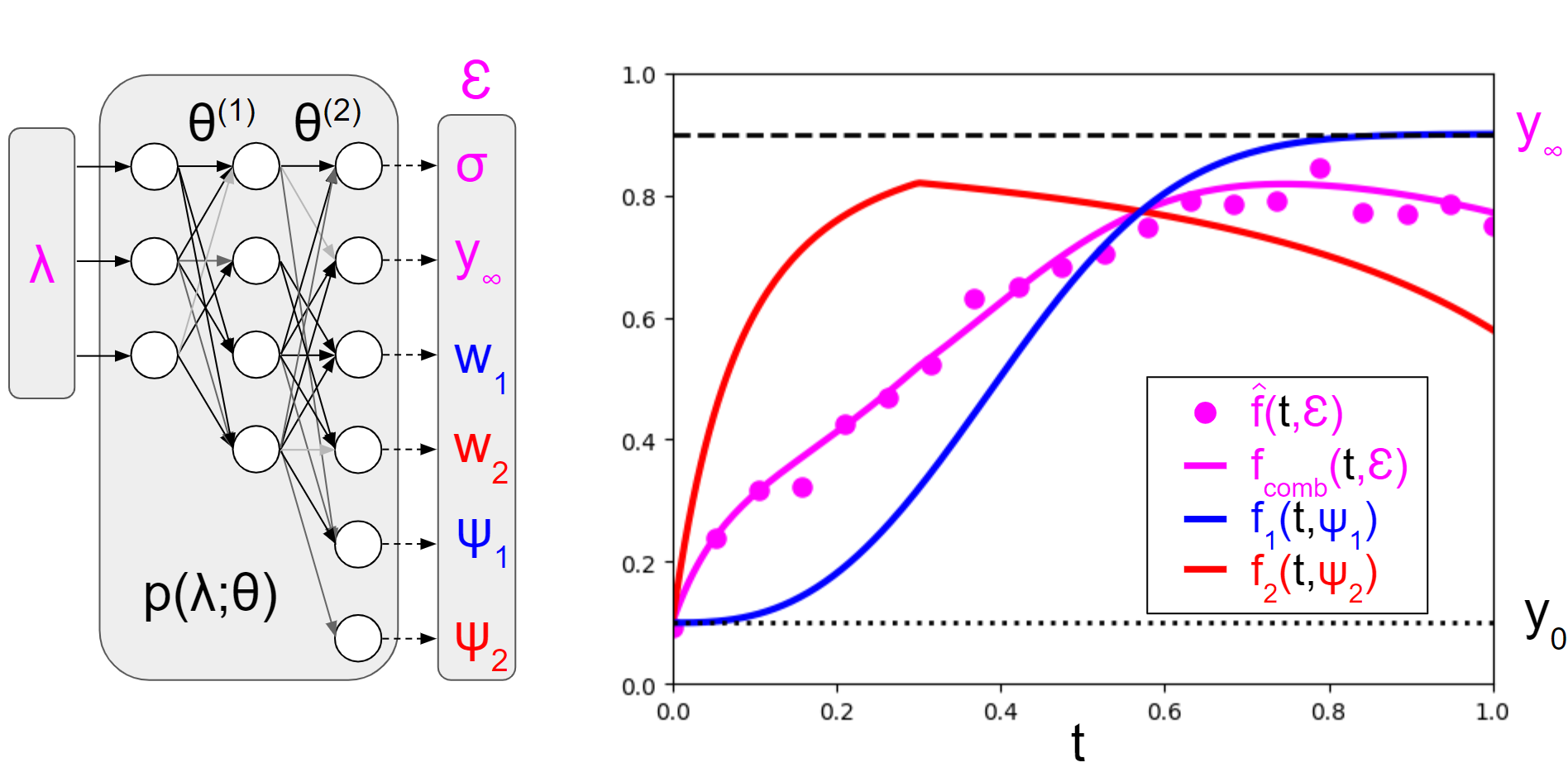
Figure 2: Diagram for the prior data model described in Section 4.1 that was used to generate data for meta-training FT-PFN. On the left, we have the randomly initialized neural network $p$ that models the relationship between a hyperparameter setting $\lambda$ and its learning curve (shown in pink), whose output parameterizes a curve model $\hat{f}$ that is a linear combination of $K$ (=2 in this illustration) basis functions (shown in red and blue) with added $\lambda$-specific Gaussian noise with variance $\sigma^{2}$.

However, unlike these previous works, we do not train the parameters $\theta$ of this neural network. Instead, we randomly initialize the network, to represent a task-specific relationship between hyperparameters and their learning curves, which we then use to generate data for training FT-PFN. This can be viewed as generating samples from a Bayesian Neural Network (BNN) prior, meta-training FT-PFN to emulate LCNet-like BNN inference through in-context learning. As for $p$, we adopt the same architecture and initialization procedure for the BNN prior used by Müller et al. (2023) in the context of BB-BO. The only difference here is that $p$ has $|\mathcal{E}|$ outputs, one for each parameter of our curve model $\hat{f}$, as opposed to a single output (model performance after a full training run). As for $\hat{f}$, following Domhan et al. (2015), Klein et al. (2017) and Adriaensen et al. (2023), we model learning curves as a linear combination of $K$ basis functions $f_{k}$, with additive Gaussian noise, i.e.,

$$\begin{split}\hat{f}(t,\mathcal{E})\sim\mathcal{N}\left(\hat{f}_{comb}(t,\mathcal{E}),{\sigma^{2}}\right)\text{\quad with}\\ f_{comb}(t,\mathcal{E})=y_{0}+(y_{\infty}-y_{0})\cdot\sum_{k=1}^{K}w_{k}f_{k}(t,\Psi_{k})\\ \text{and \quad}{\color[rgb]{0,0,0}p(\lambda;\theta)=\mathcal{E}=\left(\sigma,y_{\infty},w_{1},\ldots,w_{K},\Psi_{1},\ldots,\Psi_{K}\right)}\end{split}$$ (3)

where $y_{0}$ is the model performance after 0 training steps, and $y_{\infty}$ that at convergence. $w_{k}$ the weight of basis curve $f_{k}$, and $\Psi_{k}$ its the basis function specific parameters. Here, we adopt four different basis functions ($K=4$), each having four parameters, resulting in a total of 22 ($=|\mathcal{E}|$) parameters depending on $\lambda$ through $p$. Our four basis functions subsume the power law model used by Kadra et al. (2023), all three basis functions used by Adriaensen et al. (2023), and 9 of the 11 basis functions originally proposed by Domhan et al. (2015). Furthermore, unlike those considered in previous works, our basis functions can have a breaking point (Caballero et al., 2023) at which convergence stagnates or performance diverges, resulting in a more heterogeneous and realistic model.

Further details about meta-training FT-PFN can be found in Appendix A, including the basis curves, their parameters, and illustrations of samples from our learning curve prior (Appendix A.1); the specific procedure we use for generating our meta-training data (Appendix A.2); and the architecture and hyperparameters used (A.3).

4.2 Dynamic Acquisition Function (MFPI-random)

Following the Freeze-Thaw Bayesian Optimization framework (Section 3.2), we continue training the configuration $\lambda\in\Lambda$ that maximizes some acquisition function. Here, we assume a general multi-fidelity (MF) acquisition function (AF) represented as,

$$\texttt{MF-AF}(\lambda,z~{}|~{}f_{\text{threshold}}):\Lambda\times~{}\mathcal{Z}\rightarrow\mathbb{R}\text{,}$$ (4)

where AF is a general acquisition function, $\lambda\in\Lambda$ a hyperparameter configuration, $z\in\mathcal{Z}$ the fidelity (e.g. number of training steps), and $f_{\text{threshold}}$ a function of $f_{\text{best}}$ (best observed performance). For example, fixing $z=b_{\text{max}}$ and $f_{\text{threshold}}=f_{\text{best}}$, recovers a vanilla AF such as Expected Improvement (EI) or Probability of Improvement (PI) (Mockus et al., 1978).

The quality of uncertainty calibration in surrogate predictions depends on the task, surrogate training set quality, and extrapolation length (horizon). Meanwhile, the AF score is calibrated by an improvement threshold. In our work, we choose PI as the base AF as it is less likely to drive search towards high uncertainty regions along the hyperparameter and fidelity subspaces. Instead of using a fixed threshold or a fixed extrapolation horizon for this PI calculation, we explore a range of possible thresholds and horizons by random sampling from either fixed or problem-specific bounds. Such sampling procedure is undertaken every iteration and is akin to an acquisition selection from a portfolio of different PIs. In contrast to integrating over all thresholds (leading to Expected Improvement, EI), this allows for greater diversification in the exploration process. We posit that this hedging with a portfolio of AFs in each iteration benefits freeze-thaw setups where queries are more granular than standard BO. The result is a simple, parameter-free AF with a balanced exploration-exploitation trade-off,

$$\texttt{MFPI-random}(\lambda,z^{\text{rand}}~{}|~{}f_{\text{threshold}}^{\text{rand}}):\Lambda\times~{}\mathcal{Z}\rightarrow\mathbb{R}\text{,}$$ (5)

which evaluates to the predicted likelihood that a candidate configuration $\lambda\in\Lambda$ after $z^{\text{rand}}$ more steps of training obtains a model exceeding the $f_{\text{threshold}}^{\text{rand}}$ performance threshold, where $z^{\text{rand}}\sim\mathcal{U}(1,b_{\text{max}})$ is the sampled extrapolation horizon, and $f_{\text{threshold}}^{\text{rand}}=f_{\text{best}}\cdot(1-\tau)$, with $log_{10}(\tau)\sim\mathcal{U}(-4,-1)$ as the sampled scaling for the threshold. Further details, as well as pseudo code (Algorithm 2) can be found in Appendix A.4.

Table 1: Comparison of FT-PFN, a variant of FT-PFN that excludes hyperparameters, DyHPO and DPL across three benchmarks. Values represent the median over tasks of the log-likelihood and mean squared error (MSE) as well as the runtime of predictions.

		LCBench		PD1		Taskset		Runtime (s)
# samples	Method	Log-likelihood	MSE	Log-likelihood	MSE	Log-likelihood	MSE
	DPL	$-14.577$	$0.007$	$-13.384$	$0.043$	$-26.011$	$0.005$	$17.686$
400	DyHPO	$-0.481$	$0.042$	$-0.573$	$0.104$	$-0.465$	$0.009$	$16.860$
	FT-PFN (no HPs)	$1.649$	$0.008$	$0.983$	$0.028$	$2.860$	$0.005$	$0.215$
	FT-PFN	$1.876$	$0.005$	$0.925$	$0.030$	$2.934$	$0.004$	$0.225$
	DPL	$-13.291$	$0.007$	$-11.721$	$0.037$	$-21.779$	$0.005$	$33.480$
800	DyHPO	$-0.426$	$0.031$	$-0.510$	$0.088$	$-0.419$	$0.008$	$64.809$
	FT-PFN (no HPs)	$1.701$	$0.007$	$1.103$	$0.024$	$2.835$	$0.005$	$0.527$
	FT-PFN	$2.044$	$0.004$	$1.072$	$0.025$	$2.975$	$0.004$	$0.541$
	DPL	$-11.983$	$0.007$	$-11.017$	$0.035$	$-20.350$	$0.004$	$41.956$
1000	DyHPO	$-0.368$	$0.012$	$-0.457$	$0.071$	$-0.381$	$0.008$	$59.949$
	FT-PFN (no HPs)	$1.763$	$0.007$	$1.120$	$0.024$	$2.877$	$0.005$	$0.687$
	FT-PFN	$2.118$	$0.004$	$1.133$	$0.024$	$3.016$	$0.004$	$0.719$
	DPL	$-11.333$	$0.007$	$-10.353$	$0.033$	$-17.760$	$0.004$	$56.576$
1400	DyHPO	$-0.361$	$0.011$	$-0.438$	$0.061$	$-0.374$	$0.008$	$112.168$
	FT-PFN (no HPs)	$1.733$	$0.007$	$1.225$	$0.021$	$2.874$	$0.005$	$1.084$
	FT-PFN	$2.137$	$0.003$	$1.201$	$0.022$	$3.042$	$0.004$	$1.130$
	DPL	$-9.182$	$0.007$	$-9.263$	$0.035$	$-13.712$	$0.004$	$73.435$
1800	DyHPO	$-0.365$	$0.009$	$-0.437$	$0.058$	$-0.381$	$0.008$	$166.491$
	FT-PFN (no HPs)	$1.753$	$0.006$	$1.251$	$0.019$	$2.858$	$0.005$	$1.635$
	FT-PFN	$2.199$	$0.003$	$1.192$	$0.022$	$3.057$	$0.004$	$1.715$

5 Experiments

In this section, we compare ifBO to state-of-the-art multi-fidelity freeze-thaw Bayesian optimization methods. To this end, we first assess FT-PFN in terms of the quality and cost of its prediction (Section 5.1). Then, we assess our approach, which combines FT-PFN with our MFPI-random acquisition function, on HPO tasks (Section 5.2). Finally, we conduct an ablation study on acquisition function used in ifBO (Section 5.3).

Our main baselines are both other recent freeze-thaw approaches: DyHPO (Wistuba et al., 2022) and DPL (Kadra et al., 2023). We use the publicly available implementations for DyHPO and DPL with default hyperparameter values.

We conduct our experiments on three benchmarks: LCBench (Zimmer et al., 2021), PD1 (Wang et al., 2021), and Taskset (Metz et al., 2020). These benchmarks, covering different architectures (Transformers, CNNs, MLPs) and tasks (NLP, vision, tabular data), are commonly used in the HPO literature. A detailed overview of the tasks included in each benchmark is presented in Appendix B.

5.1 Cost and Quality of Predictions

In this section, we compare the predictive capabilities of FT-PFN to that of existing surrogate models, including the deep Gaussian process of DyHPO (Wistuba et al., 2022) and the deep ensemble of power laws model of DPL (Kadra et al., 2023). We also consider a variant of FT-PFN trained on the same prior, but not taking the hyperparameters as input (referred to as ”no HPs”). This variant bases its predictions solely on a set of partially observed learning curves.

Evaluation procedure:

From a given benchmark, we sample both a set of partial curves, where each curve has its own set of target epochs. The selection process is strategically designed to encompass a wide range of scenarios, varying from depth-first approaches, which involve a smaller number of long curves, to breadth-first approaches, where multiple shorter curves are explored. Additional details on the sampling strategy can be found in Appendix A.2. To assess the quality of the predictions, we utilize two metrics: log-likelihood (log-score, the higher the better), measuring the approximation of the posterior distribution ($\sim$ uncertainty calibration), and mean squared error (the lower the better), measuring the accuracy of point predictions. We also report the runtime, accounting for fitting and inference of each surrogate. The evaluation was run on a single Intel Xeon 6242 CPU.

Results discussion:

Table 1 presents the log-likelihood and MSE (Mean Squared Error) for each approach relative to the context sample size. As expected, we observe an increase in log-likelihood and a decrease in MSE as the context size get larger. Notably, FT-PFN and its No HPs variant significantly outperform DPL and DyHPO in terms of log-likelihood. DPL in particular has low log-likelihood values, corresponding to a poor uncertainty estimate such as being overly confident in incorrect predictions. This may be due to the very low ensemble size ($=5$) adopted by (Kadra et al., 2023) compounded by their strong power law assumption. On the other hand, DyHPO struggles with low log-likelihood due to its inability to extrapolate beyond a single step effectively. Regarding MSE, FT-PFN generally surpasses the baselines in LCBench and PD1, performing comparably to DPL on Taskset.

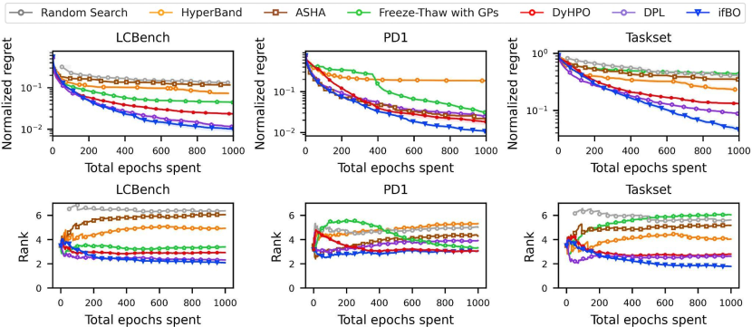
Figure 3: Comparison of our method against state-of-the-art baselines on all 3 benchmarks. First row shows normalized regret aggregated across multiple tasks in each benchmark (See Appendix B for benchmark details, and the results per task can be found in Appendix E). Second row shows the average ranks of each method.

Beyond the impressive log-likelihood and MSE results, our approach also yield significant speed advantages over the baseline methods. Importantly, FT-PFN maintains superiority in quality and speed for inferences with more than $1000$ samples as a context without not being trained in this regime. Depending on the context sample size, our method achieves speedups ranging from $10\times$ to $100\times$ faster than DPL and DyHPO.

5.2 Assessment of HPO performance

In this section, we present an extensive empirical comparison, showing the merits of our method on HPO tasks across a variety of tabular benchmarks (see Appendix B) in the low budget regime. Additionally to DPL and DyHPO, we include Hyperband, ASHA, Gaussian Process-based FT-BO (using DyHPO’s one-step EI acquisition function) and uniform random search, as baselines. Each algorithm is allocated a total budget of 1000 steps for every task, which corresponds to 20 full trainings on LCBench and Taskset  with each task being repeated 10 times, each time starting from a different random configuration (see Algorithm 1). We report two complementary metrics: The normalized regret, capturing performance differences, and the average rank of each method, capturing the relative order. Formally, the normalized regret corresponds to a $[0,1]$ normalization of the observed error w.r.t to the best (lowest) and worst (highest) errors recorded by all algorithms on the task.

Results discussion:

Figure 3 presents the comparative results per benchmark family. The results validate the superiority of freeze-thaw approaches (ifBO, DyHPO, and DPL) compared to standard approaches (Hyperband, ASHA, and random search) for low-budget settings. Most notably, these results establish the promise of ifBO, which either outperforms (on LCBench and Taskset) or competes closely (on PD1) with DPL and DyHPO. ifBO is also consistently the best on average rank across all benchmarks (see Appendix C.2, Figure 7). Appendix E (Figures 11-16) offers a closer look at the raw error metrics for each algorithm per task. These detailed results collectively confirm the robustness of ifBO for HPO tasks, showing its ability to compete if not outperform the most competitive baselines.

5.3 Ablation on Acquisition

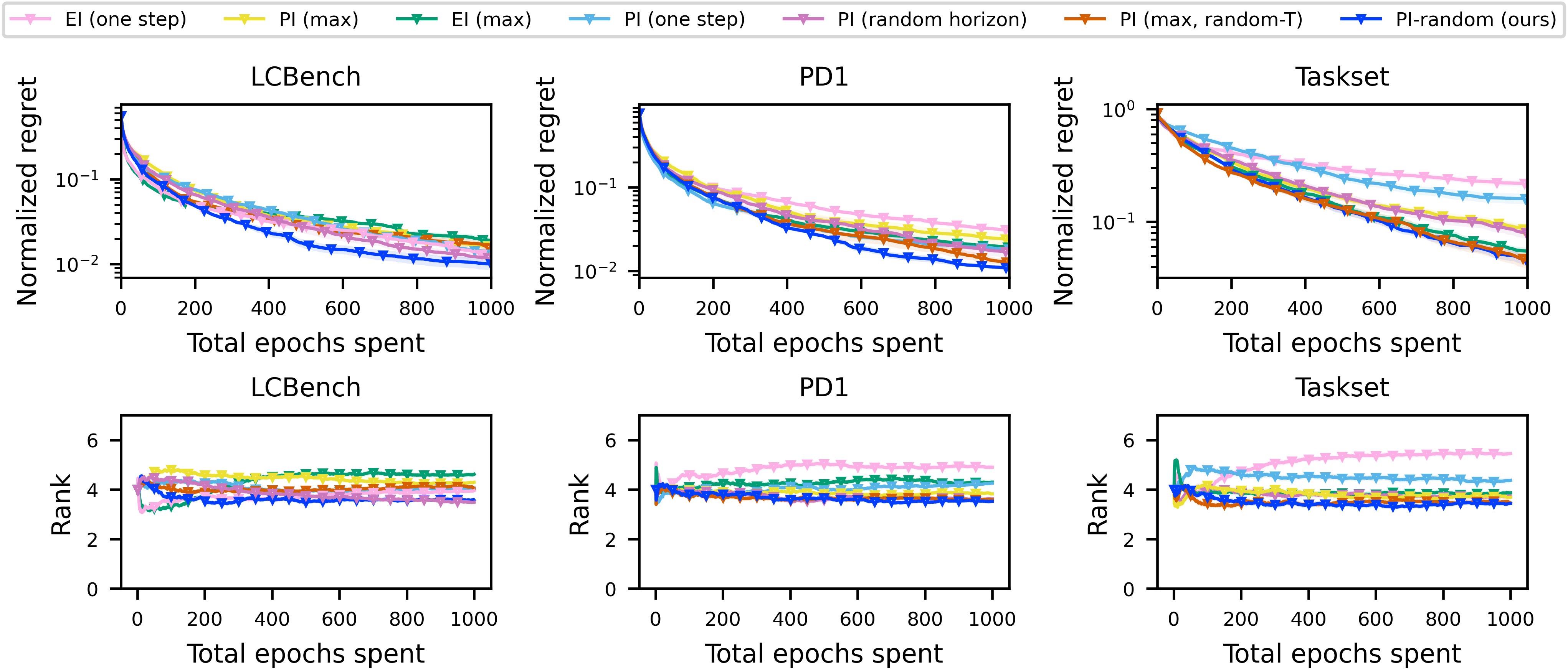
Figure 4: Results of an ablation study of the acquisition function in ifBO on each benchmark family. First row shows normalized regret aggregated across multiple tasks in each benchmark (Appendix B). Second row shows the average ranks of each method.

In this section, we evaluate how ifBO performs in combination with other acquisition functions and aim to assess to what extent our novel acquisition function described in Section 4.2 contributes to its HPO success. To this end, we consider ifBO variants combining FT-PFN with and comparing performance against the EI-based acquisitions used in prior-art (Wistuba et al., 2022; Kadra et al., 2023), i.e., EI (one step) predicting one step in the future (DyHPO), and EI (max) predicting at the highest budget $b_{max}$ (DPL). We also include their PI counterparts PI (one step) and PI (max), as well as variants of MFPI-random that only vary the prediction horizon, PI (random horizon) with $T=0$, or only vary the threshold, PI (max, random-T) with $h=b_{max}$. Apart from the methods compared, the experimental setup is identical to that in Section 5.2.

Results discussion:

Figure 4 shows the comprehensive results for our ifBO variants for each of the benchmarks, in terms of average ranks and average normalized regrets, aggregated across all tasks. Generally, we find that performance varies strongly between acquisitions, suggesting this choice is at least as important for HPO success as our surrogate’s superior predictive quality. In particular, we find that combinations with the EI-based acquisitions EI (one step) and EI (max) proposed in prior-art, are amongst the worst-performing variants, both in terms of rank and regret. For example, EI (max) fails on LCBench and PD1, while EI (one step) fails on PD1 and Taskset. Curiously, these trends do not seem to extend to our baselines, e.g., DPL using EI (max) performs strongly on LCBench and DyHPO using EI (one step) performs strongly on PD1. We conjecture that this failure is related to the (justified) lack of confidence FT-PFN has about its predictions, as is evident by the superior log-scores in Table 1. As a result, the predicted posterior will be heavy-tailed, resulting in the high EI values for those configurations our predictions are least confident for. While this drives exploration, in the very low budget regime, it can easily lead to a catastrophic failure to exploit. Overall, we find that while some variants are successful at specific tasks in early stages of the optimization, none exhibit the same robustness in performance across benchmarks, making MFPI-random the clear winner.

We perform comparable ablation studies for DPL and DyHPO, as detailed in Appendix C.3, to demonstrate the benefits of randomizing the horizon and the threshold.

6 Conclusion

In this paper, we proposed FT-PFN a novel surrogate for freeze-thaw Bayesian optimization. We showed that the point and uncertainty estimates produced by FT-PFN through in-context learning are superior to those obtained by fitting/training recently proposed deep Gaussian process (Wistuba et al., 2022) and deep power law ensemble (Kadra et al., 2023) models, while being over an order of magnitude faster. We presented the first-ever empirical comparison of different freeze-thaw implementations. Our results confirm the superiority of these HPO methods, in the low-budget regime, and show that our in-context learning approach is competitive with the state-of-the-art.

Despite our promising results, we admit that attaining the sample efficiency required to scale up to modern deep learning (e.g., LMM pretraining) remains a challenging endeavor. Future work should attempt to extend our approach to take advantage of additional sources of prior information, e.g., to do in-context meta-learning, leveraging learning curves on related tasks (Ruhkopf et al., 2022); to incorporate user priors (Müller et al., 2023; Mallik et al., 2023); and additional information about the training process (e.g., gradient statistics). An alternative to scaling up is scaling in parallel. Here, we expect our in-context learning approach to reduce the overhead further, as the online learning/refitting stage occurs on the critical path, while in-context learning during prediction can easily be parallelized. Finally, the current FT-PFN model has some limitations. First, it requires the performance metric and each hyperparameter value to be normalized in $[0,1]$; and supports up to 10 hyperparameters. While we believe that this is reasonable, future work building systems should push these limits, train larger models, on more data, and explore ways to scale to larger context sizes. In summary, there is a lot left unexplored, and we hope that the relative simplicity, efficiency, and public availability of our method, lowers the threshold for future research in this direction.

Impact Statement

This paper presents work whose goal is to advance the field of hyperparameter optimization (HPO) in machine learning. There are many potential societal consequences of machine learning, none which we feel must be specifically highlighted here. We would, however, like to highlight that our work makes HPO more robust and efficient, and will thus help make machine learning more reliable and sustainable.

Appendix A Further Details about ifBO

A.1 The Learning Curve Prior

In this section, we continue the discussion of our learning curve prior defined by Equation 2:

$$\begin{split}\hat{f}(t,\mathcal{E})\sim\mathcal{N}(\hat{f}_{comb}(t,\mathcal{E}),{\sigma^{2}})\text{\quad with \quad}f_{comb}(t,\mathcal{E})=y_{0}+(y_{\inf}-y_{0})\cdot\sum_{k=1}^{K}w_{k}*f_{k}(t,\Psi_{k})\\ \text{and \quad}p(\lambda;\theta)=\mathcal{E}=\{\sigma,y_{\inf}\}\cup\{w_{k}\}_{k=1}^{K}\cup\bigcup\limits_{k=1}^{K}\Psi_{k}\end{split}$$ (6)

Each of the basis curves takes the form

$$f_{k}(t,\Psi_{k})=f_{k}^{\prime}(x_{t},\Psi_{k})\text{\quad with \quad}x_{t}=\frac{1}{b_{max}}\cdot\begin{cases}t&\text{if }t\leq x_{sat,k}^{\lambda}\\ r_{sat,k}^{\lambda}(t-x_{sat,k})+x_{sat,k}&\text{if }t>x_{sat,k}^{\lambda}\end{cases}$$ (7)

where $f_{k}$ has the following four parameters $\Psi_{k}$:

$\alpha_{k}$

The skew of the curve, determining the convergence rate change over time.

$x_{sat,k},\,y_{sat,k}$

The point at which model performance saturates and the convergence rate is suddenly reduced.

$r_{sat,k}$

The reduced convergence rate after saturation, which can be negative, modeling divergence.

and $f_{k}^{\prime}(x_{t},\theta_{k})$ is a [0,1] bounded monotonic growth function. The formulas for these growth functions, alongside the target distributions of their parameters, are listed in Table 2.

Reference name	Formula $f_{k}(x_{t},\Psi_{k})$	Prior $p(\Psi_{k})$
$pow\textsubscript{4}$	$((\epsilon_{1}^{\frac{-1}{\alpha_{1}}}-1)*\frac{x_{t}}{x_{sat,1}}+1)^{-\alpha_{1}}$	$\ln(\alpha_{1})\sim\mathcal{N}(1,1)$	$\log_{10}(x_{sat,k})\sim\mathcal{N}(0,1),\,\forall\,k$
$exp\textsubscript{4}$	$(\epsilon_{2})^{(\frac{x_{t}}{X_{sat,2}})^{\alpha_{2}}}$	$\ln(\alpha_{2})\sim\mathcal{N}(0,1)$	$\ln(\epsilon)\sim\mathcal{N}(-5,1),\,\forall\,k$
$ilog\textsubscript{4}$	$\frac{\ln(\alpha_{3})}{\ln((\alpha_{3}^{\frac{1}{\epsilon_{3}}}-\alpha_{3})\frac{x_{t}}{X_{sat,3}}+\alpha_{3})}$	$\ln(\alpha_{3}-1)\sim\mathcal{N}(-4,1)$	$y_{sat,k}=y_{\inf}-\epsilon\cdot(y_{\inf}-Y_{0}),\,\forall\,k$
$hill\textsubscript{4}$	$\frac{1}{(\frac{x_{t}}{X_{sat,4}})^{\alpha_{4}}(\frac{1}{\epsilon_{4}}-1)+1}$	$\ln(\alpha_{4})\sim\mathcal{N}(0.5,0.25)$	$1-r_{sat,k}\sim Exp(1),\,\forall\,k$

Table 2: The formulas for each of the four basis functions in our curve prior. Note that each of them are normalized to start at 1, converge to 0, and pass through the saturation point.

Finally, note that given these choices, we have $f_{comb}(t,\mathcal{E})\in[0,1]$ and we clip the Gaussian noise in $\hat{f}(t,\mathcal{E})$ in the same range. As a consequence, if performance does not naturally fall in this range, it must be normalized before passing it to FT-PFN. Examples of collections of curves generated using this prior can be found in Figure 5.

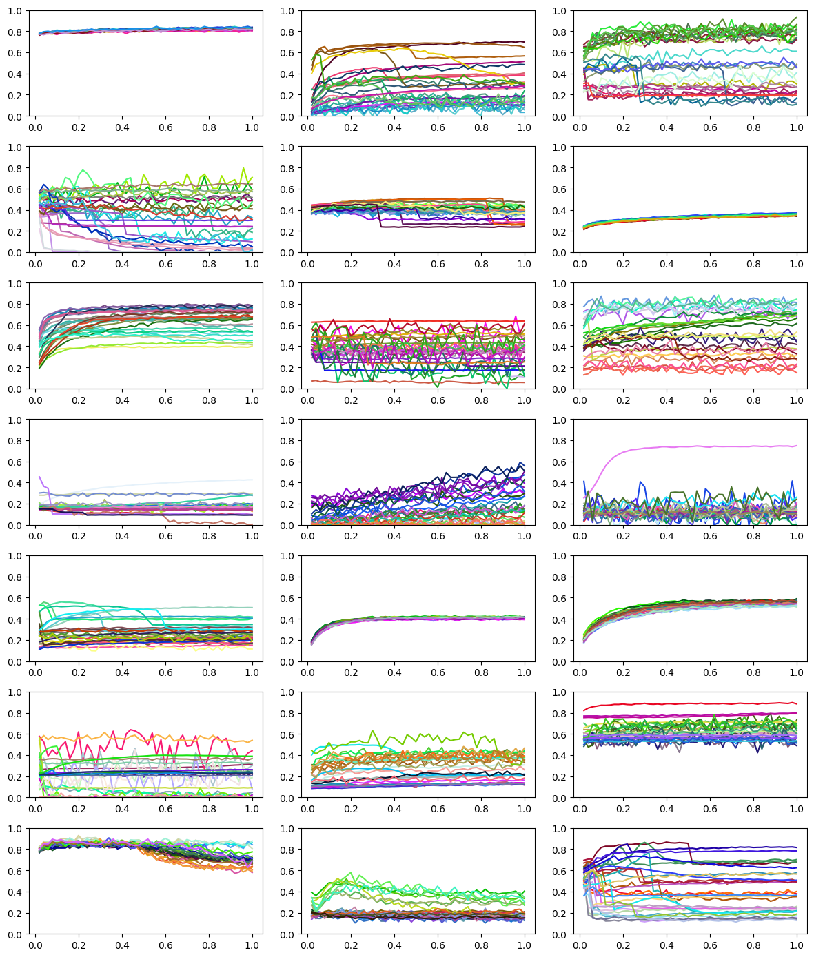
Figure 5: 21 i.i.d. samples of the FT-PFN prior, i.e., synthetically generated collections of learning curves for the same task using different hyperparameter configurations. In these examples, we consider 3 hyperparameters that are mapped onto the color of the curves, such that runs using similar hyperparameters, have similarly colored curves. We observe correlations, in varying degrees, between curves on the same task, especially with similar hyperparameter configurations.

A.2 Meta-training Data Generating Procedure

A single meta-training example in our setting corresponds to a training set $D_{train}$ and test set $D_{test}$, where ${D_{train}=\{(\lambda,t),f(\lambda,t)\}_{t=1,\forall\lambda\in\Lambda}^{b_{\lambda}^{\prime}}}$ corresponds to the (synthetic) partial learning curves observed thus far (i.e., the analog of $H$ at test time) and $D_{test}\subseteq{\lambda,t,\,f(\lambda,t)\}_{\lambda\in\Lambda,\,b_{max}\geq t>b_{\lambda}}}$ the extrapolation targets we want FT-PFN to predict. To keep the input size of FT-PFN fixed we choose $|D_{train}|+|D_{test}|=N$ and vary the size of $|D_{train}|\sim\mathcal{U}(0,B-1)$. As $b_{max}$ varies in practice, we sample it log-uniformly in $[1,1000]$. Note that in the special case $b_{max}=1$, we train FT-PFN for BB-BO. $\Lambda={\lambda_{i}}_{i}=1^{N}$ is our synthetic configuration space with $\lambda_{i}\sim\mathcal{U}(0,1)^{d}$, with $|\lambda_{i}|=m\sim\mathcal{U}(0,M)$ the dimensionality of our configuration space. We determine $b_{\lambda}$ by sampling a bag of $|D_{train}|$ elements from $\Lambda$ proportionally to weights $\{w_{\lambda}\}_{\lambda\in\Lambda}$ that follow a Dirichlet distribution with $\log_{10}(\alpha)\sim\mathcal{U}(-4,-1)$ resulting in heterogeneous budget allocations that vary from breadth-first to depth-first. We use the same weights to sample another bag of $|D_{test}|$ determining the number of extrapolation targets for each $\lambda$, where each target is chosen $\mathcal{U}(b_{\lambda},b_{max})$. Finally, to generate the corresponding $f(\lambda_{i},t_{i})$, we first instantiate the random variables that are task-specific but do not depend on $\lambda$, i.e., $y_{0}\sim\mathrm{Beta}(1,2)$, and the architecture and weights $\theta$ of the neural network $p$. Finally, we determine $f(\lambda_{i},t_{i})=\hat{f}(t_{i},p(\lambda;\theta))$.

Limitations:

With these modeling choices come some limitations. First, FT-PFN is trained for HPO budgets $B\leq N=1,000$; requires the performance metric $f$ and each hyperparameter value to be normalized in [0,1]; and supports up to $M=10$ hyperparameters.

A.3 Architecture and Hyperparameters

Following Müller et al. (2022), we use a sequence Transformer (Vaswani et al., 2017) for FT-PFN and treat each tuple ($\lambda$, $t$, f($\lambda$, $t$)) (for train) and ($\lambda$, $t$) (for test) as a separate position/token. We do not use positional encoding such that we are permutation invariant. FT-PFN outputs a discretized approximation of the PPD, each output corresponding to the probability density of one of the equal-sized bins. We set the number of bins/outputs to 1,000. For the transformer, we use 6 layers, an embedding size of 512, four heads, and a hidden size of 1,024, resulting in a total of 14.69M parameters. We use a standard training procedure for all experiments, minimizing the cross-entropy loss from Equation 1 on 2.0M synthethic datasets generated as described in Section A.2, using the Adam optimizer (Kingma et al., 2015) (learning rate 0.0001, batch size 25) with cosine annealing (Loshchilov & Hutter, 2017) [Loshchilov and Hutter, 2017] with a linear warmup over the first 25% epochs of the training. Training took roughly 8 GPU hours on an RTX2080 GPU and the same FT-PFN is used in all experiments described in Section 5, without any retraining/fine-tuning.

A.4 Acquisition function

Algorithm 2 describes the acquisition loop in ifBO. The two parameters in Equation 4 are chosen randomly, with Probability Improvement (PI) (Mockus et al., 1978) as the base acquisition function (AF). In each iteration of ifBO (L3-L9 in Alg. 1), Alg. 2 is invoked once. In each such run, the random horizon $z$ and the scaled threshold of improvement $f_{\text{threshold}}$ are sampled once. This process can be seen as instantiating an acquisition function from a portfolio of multi-fidelity PIs. The choice of PI, the multi-fidelity component of extrapolating hyperparameters, and the random selection of an acquisition behaviour lends the naming of this acquisition function, MFPI-random. For each candidate evaluated ($\hat{\lambda}\in\Lambda$), the posterior is inferred given the surrogate for a hyperparameter $\hat{\lambda}$ at a total horizon of its current observed length in unit steps ($b_{\hat{\lambda}}$) $+$ the sampled horizon ($z$). The candidate with the highest obtained PI score is returned as the candidate solution to query next in the main Alg. 1 loop.

Algorithm 2 MFPI-random

Input: configuration space $\Lambda$,
probabilistic surrogate $\mathcal{M}$,
history of observations $H$,
maximal steps $b_{\text{max}}$

Output: $\lambda^{\prime}\in\Lambda$, next query

Procedure MFPI-random($\Lambda$, ${\color[rgb]{0,0,0}\mathcal{M}}$, $H$, $b_{\text{max}}$):

  $f_{\text{best}}\leftarrow$ best score seen in $H$

  $z\sim\mathcal{U}(1,b_{\text{max}})$random horizon

  $\tau\sim\mathcal{U}(-4,-1)$random threshold scaling

  $f_{\text{threshold}}=f_{\text{best}}\cdot(1-10^{\tau})$

  $D\leftarrow\{\}$

  for all $\hat{\lambda}\in\Lambda$ do

     $y^{\prime}\leftarrow$ $\mathds{P}({\color[rgb]{0,0,0}\mathcal{M}}(\hat{\lambda},~{}b_{\hat{\lambda}}+z)\leq f_{\text{threshold}})$

     $D\leftarrow{}D\bigcup{}\{(\hat{\lambda},~{}y^{\prime})\}$

  end for

  return $\operatorname*{arg\!max}_{\lambda\in\Lambda}\{(\lambda,y)\}_{(\lambda,y)\in D}$

Appendix B Benchmarks

Below, we enumerate the set of benchmarks we have considered. These benchmark cover a variety of optimization scenarios, including the model being optimized, the task for which it’s being trained on, and the training metric with which to optimize hyperparameters with respect to. Notably, each of these benchmarks are tabular, meaning that the set of possible configurations to sample from is finite.

This choice of benchmarks is largely dictated by following the existing benchmarks used in prior work, especially the two primary baselines with which we compare to, DyHPO and DPL.

These benchmarks were provided using mf-prior-bench.

• LCBench (Zimmer et al., 2021) [DyHPO, DPL] - We use all 35 tasks available which represent the 7 integer and float hyperparameters of deep learning models from AutoPyTorch. Each task represents the 1000 possible configurations, trained for 52 epochs on a dataset taken from the AutoML Benchmark (Gijsbers et al., 2019). We drop the first epoch as suggested by the original authors.

  Table 3: The 7 hyperparameters for all LCBenchtasks.

  name	type	values	info
  batch_size	integer	$[16,512]$	log
  learning_rate	continuous	$[0.0001,0.1]$	log
  max_dropout	continuous	$[0.0,1.0]$
  max_units	integer	$[64,1024]$	log
  momentum	continuous	$[0.1,0.99]$
  num_layers	integer	$[1,5]$
  weight_decay	continuous	$[1e\mbox{-}05,0.1]$

• Taskset (Metz et al., 2020) [DyHPO, DPL] This set benchmark provides 1000 diverse task on a variety of deep learning models on a variety of datasets and tasks. We choose the same 12 tasks as used in the DyHPO experimentation which consists of NLP tasks with purely numerical hyperparameters, mostly existing on a log scale. We additionally choose a 4 hyperparameter variant and an 8 hyperparameter variant, where the 4 hyperparameter variant is a super set of the former. This results in 24 total tasks that we use for the Taskset benchmark.

  One exception that needs to be considred with this set of benchmarks is that the optimizers must optimize for is the model’s log-loss. This metric has no upper bound, which contrasts to all other benchmarks, where the bounds of the metric are known a-priori. We note that in the DyHPO evaluation setup, they removed diverging curves as a benchmark preprocessing step, essentially side-stepping the issue that the response function for a given configuration mays return nans or out-of-distribution values. As our method requires bounded metrics, we make the assumption that a practitioner can provide a reasonable upper bound for the log loss that will be observed. By clampling to this upper bound, this effectively shrinks the range of values that our method will observe. As we are in a simulated benchmark setup, we must simulate this a-priori knowledge. We take the median value of at epoch 0, corresponding to the median log loss of randomly initialized configurations that have not yet taken a gradient step. Any observed value that is nan or greater will then be clamped to this upper bound before being fed to the optimizer.

  Table 4: The 4 hyperparameter search space for Taskset.

  name	type	values	info
  beta1	continuous	$[0.0001,1.0]$	log
  beta2	continuous	$[0.001,1.0]$	log
  epsilon	continuous	$[1e\mbox{-}12,1000.0]$	log
  learning_rate	continuous	$[1e\mbox{-}09,10.0]$	log

  Table 5: The 8 hyperparameter search space for Taskset.

  name	type	values	info
  beta1	continuous	$[0.0001,1.0]$	log
  beta2	continuous	$[0.001,1.0]$	log
  epsilon	continuous	$[1e\mbox{-}12,1000.0]$	log
  learning_rate	continuous	$[1e\mbox{-}09,10.0]$	log
  exponential_decay	continuous	$[9e\mbox{-}07,0.0001]$	log
  l1	continuous	$[1e\mbox{-}09,10.0]$	log
  l2	continuous	$[1e\mbox{-}09,10.0]$	log
  linear_decay	continuous	$[1e\mbox{-}08,0.0001]$	log

• PD1 (Wang et al., 2021) [DPL] These benchmarks were obtained from the output generated by HyperBO  (Wang et al., 2021) using the dataset and training setup of (Gilmer et al., 2021). We choose a variety of tasks including the tuning of large vision ResNet (Zagoruyko & Komodakis, 2016) models on datasets such as CIFAR-10, CIFAR-100 (Krizhevsky, 2009) and SVHN (Liao & Carneiro, 2022) image classification datasets, along with training a ResNet (He et al., 2016) on the ImageNet (Russakovsky et al., 2015) image classification dataset. We also include some natural language processing tasks, notable transformers train on the LM1B (Chelba et al., 2013) statistical language modelling dataset, the XFormer (Lefaudeux et al., 2022) trained on the WMT15 German-English (Bojar et al., 2015) translation dataset and also a transformer trained to sequence prediction for protein modelling on the uniref50 dataset. Lastly, we also include a simple CNN trained on the MNIST (Deng, 2012) and Fashion-MNIST (Xiao et al., 2017) datasets.

  Notably, all of these benchmarks share the same 4 deep learning hyperparameters given in table 6.

  Table 6: The 4 hyperparameters for all PD1tasks.

  name	type	values	info
  lr_decay_factor	continuous	$[0.01,0.99]$
  lr_initial	continuous	$[1e\mbox{-}05,10.0]$	log
  lr_power	continuous	$[0.1,2.0]$
  opt_momentum	continuous	$[1e\mbox{-}05,1.0]$	log

  Each benchmark ranges in the size of their learning curves, depending on the task, ranging from 5 to 1414. For each task, there are different variant based on a pair of dataset and batchsize. In total we evaluate our method on the 16 PD1 tasks below.

  • WideResnet - Tuned on the CIFAR10, CIFAR100 datasets, each with a constant batch size of $256$ and $2048$. Also included is the SVHN dataset with a constant batch size $256$ and $1024$.

  • Resnet - Tuned on ImageNet with three constant batch sizes, $256$, $512$, and $1024$.

  • XFormer - Tuned with a batch size of $2048$ on the LM1B statistical language modelling dataset.

  • Transfomer Language Modelling - Tuned on the WMT15 German-English dataset with a batch size of $64$.

  • Transformer Protein Modelling - Tuned on the uniref50 dataset with a batch size of $128$.

  • Simple CNN - Tuned on MNIST and Fashion-MNIST with constant batch sizes of $256$ and $2048$ for each of them.

Appendix C Further Ablations

C.1 Effectiveness of modeling curve divergence

As detailed in Section A.1, our curve prior is capable to model learning curve with diverging behavior. This capability is novel compared to the related works (Adriaensen et al., 2023; Klein et al., 2017; Kadra et al., 2023; Domhan et al., 2015), which are restricted to monotonic curves only. In Figure 6, we empirically show that modeling diverging curves yields a better surrogate model in terms of both extrapolation and HPO.

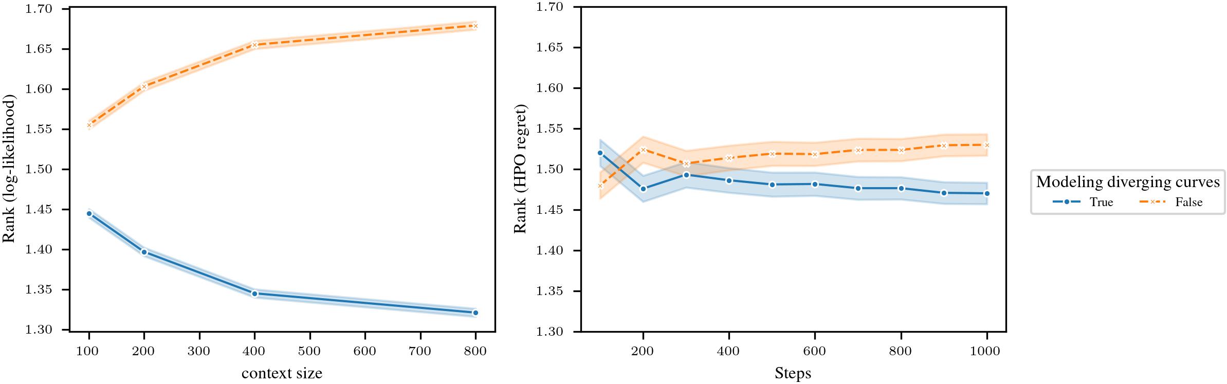
Figure 6: Comparison of the relative ranks of the performance gained by modeling divergences in ICL-FT-PFN. The plots, showing the average ranks across all the benchmarks (LCBench, PD1, and TaskSet), confirm the merits of capturing diverging curves both in terms of the quality of the predictions (log-likelihood, left) and HPO performances (regret, right).

C.2 Pairwise comparison of freeze-thaw approaches

For a fine-grained assessment of the performance of ifBO, we present a pairwise comparison with the main freeze-thaw approaches including DPL and DyHPO. This is to visualize the relative gain of performance compared to each baseline, which may have been hidden from Figure 5.2. As shown in Figure 7, our approach dominates consistently DPL and DyHPO after $\approx$ 150 steps of HPO run.

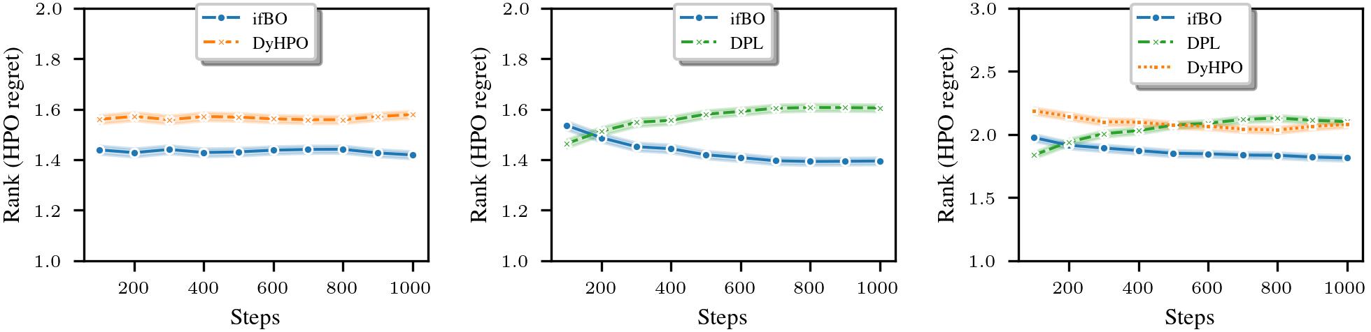
Figure 7: Comparison of relative ranks when aggregated over all benchmark families, showing strong anytime performance in both pairwise comparisons and also overall among freeze-thaw algorithms.

C.3 Acquisition function ablation of the baselines

In this section, our objective is to explore the impact of incorporating randomization into the acquisition function on the baseline methods (DPL and DyHPO). For this purpose, we assess each baseline across four distinct acquisition functions (Figure 8), each representing a different configuration of Equation 4. The variants include: (ours), where both the horizon and the threshold for improvement are randomly selected, similar to the approach in ifBO; (one-step), where the horizon and threshold for improvement are chosen as in DyHPO; (at max), where the selection criteria for the horizon and threshold follow the methodology in DPL; and (random horizon), where the horizon is randomly determined, and the threshold is set to the best value observed.

The results presented in Figure 8 confirm that the randomization technique markedly enhances the performance of methods capable of extending learning curves over many steps, such as ifBO and DPL. Furthermore, please note that only the greedy one-step acquisition function is effective for DyHPO, given that it is specifically designed for one-step ahead predictions.

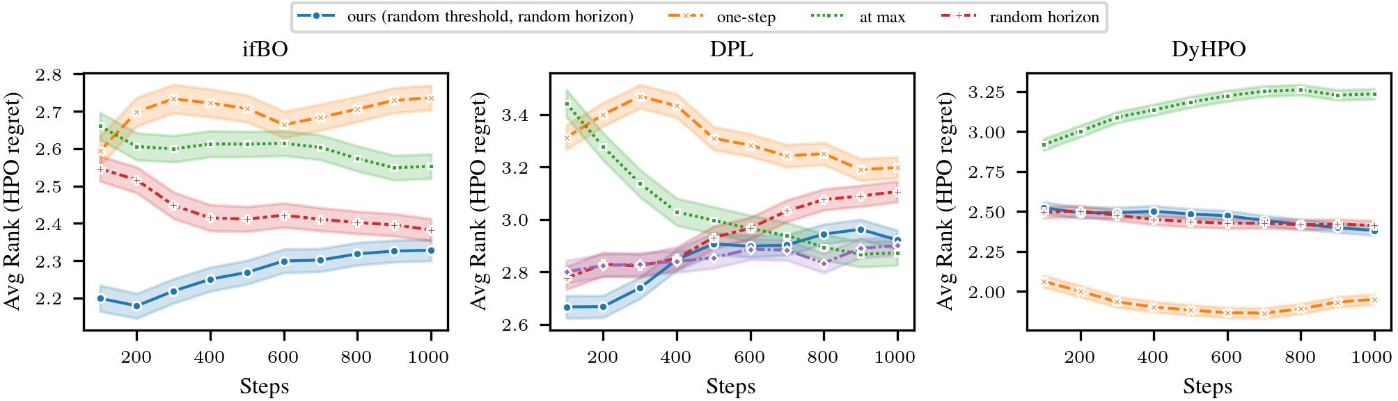
Figure 8: Relative ablation over the horizon and threshold parameters of a multi-fidelity AF (Equation 4).

C.4 Comparison of freeze-thaw approaches with MFPI-random

In Figure 9, we present a comparison of all the freeze-thaw approaches—including ours, DPL, and DyHPO—when employing our acquisition function (MFPI-random). Despite all models utilizing the same acquisition function, our model significantly outperforms those of DPL and DyHPO. This clearly indicates the crucial role our prior in achieving the final performance.

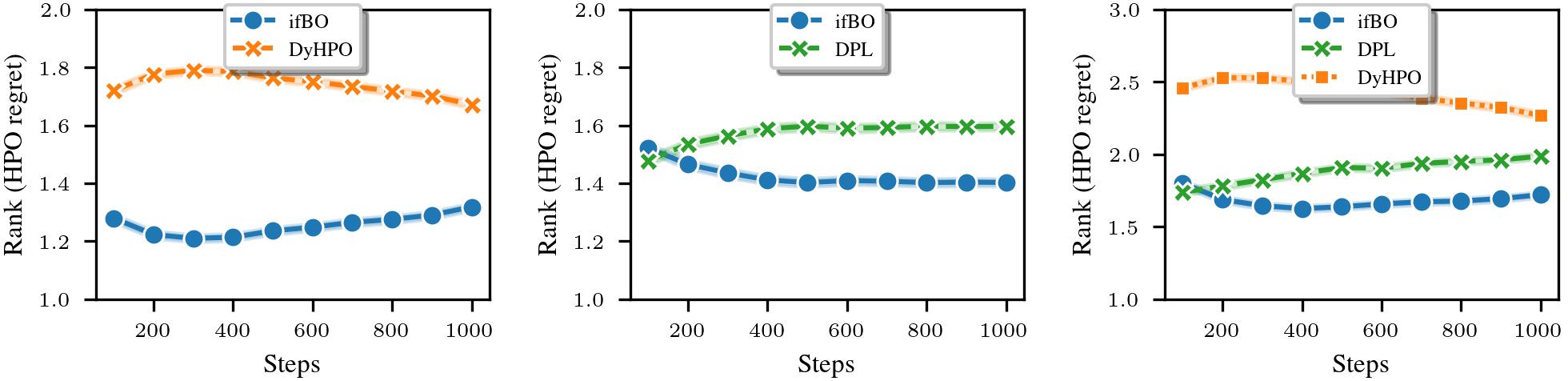
Figure 9: Comparison of freeze-thaw approaches (ifBO, DPL, and DyHPO) when using our acquisition (MFPI-random) with their specific surrogate models. The plots represent the average ranks over all benchmarks (LCBench, PD1, and Taskset). This ablation confirms that our novel surrogate (and not only our novel acquisition function) contributes significantly to the HPO performance of ifBO.

Appendix D Aggregate plots over time

Figure 10 plots Figure 3(bottom) but with the $x$-axis as cumulative wallclock time from the evaluation costs returned by the benchmark for each hyperparameter for every unit step. The overall conclusions remain over our HPO budget of $1000$ steps. ifBO is on average anytime better ranked than the freeze-thaw HPO baselines.

LCBench	PD1	TaskSet	Aggregated

Figure 10: Comparing relative rank over wallclock time (in $s$) over different benchmark families and the aggregated result overall. ifBO is on average better than the baselines, DyHPO and DPL, except for the TaskSet benchmark family where DPL starts the best but ifBO improves with more budget. Plots have been cutoff at a common $10^{5}$ seconds for fair comparison.

Appendix E Per-task HPO Plots

In Section 3.1, we presented HPO results on each of these three benchmarks in a comprehensive form, averaging rank and normalized regrets across every task in the suite. These averages may hide / be susceptible to outliers. For completeness, Figures 11-16 provide regret plots for every task in the benchmark, averaged across the 10 seeds. We find that our method consistently performs on par, or better than the best previous best HPO method, especially in later stages of the search, without notable outliers.

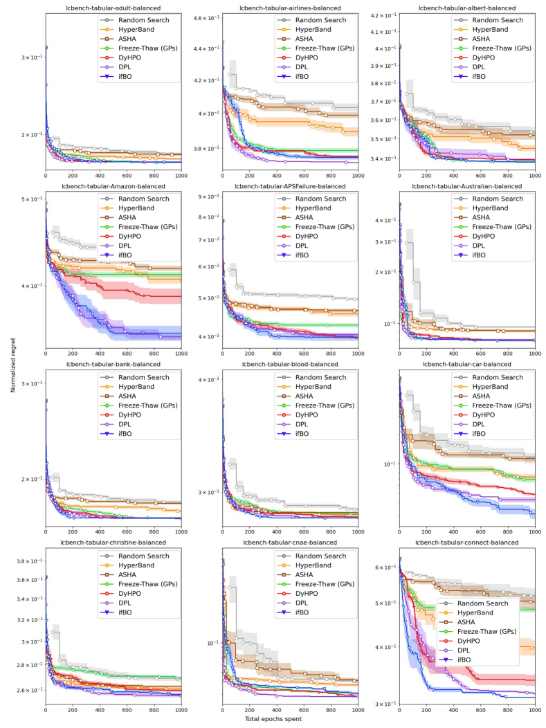
Figure 11: Per-task HPO results on LCBench

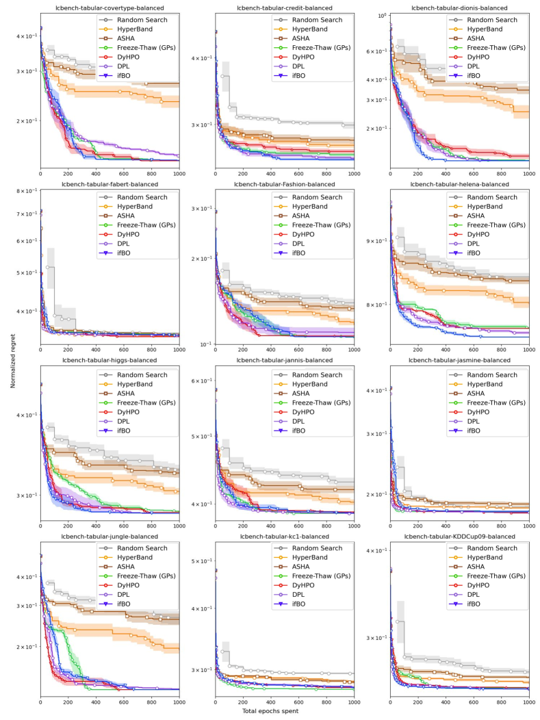
Figure 12: Per-task HPO results on LCBench (cont.)

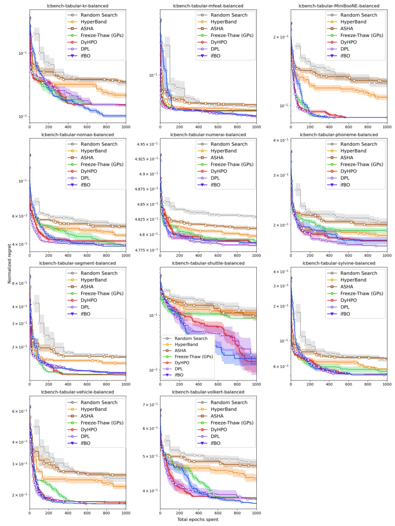
Figure 13: Per-task HPO results on LCBench (cont.)

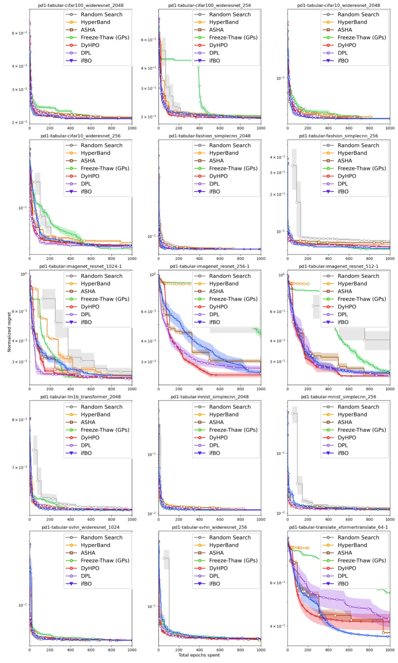
Figure 14: Per-task HPO results on PD1

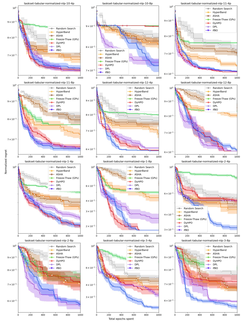
Figure 15: Per-task HPO results on Taskset

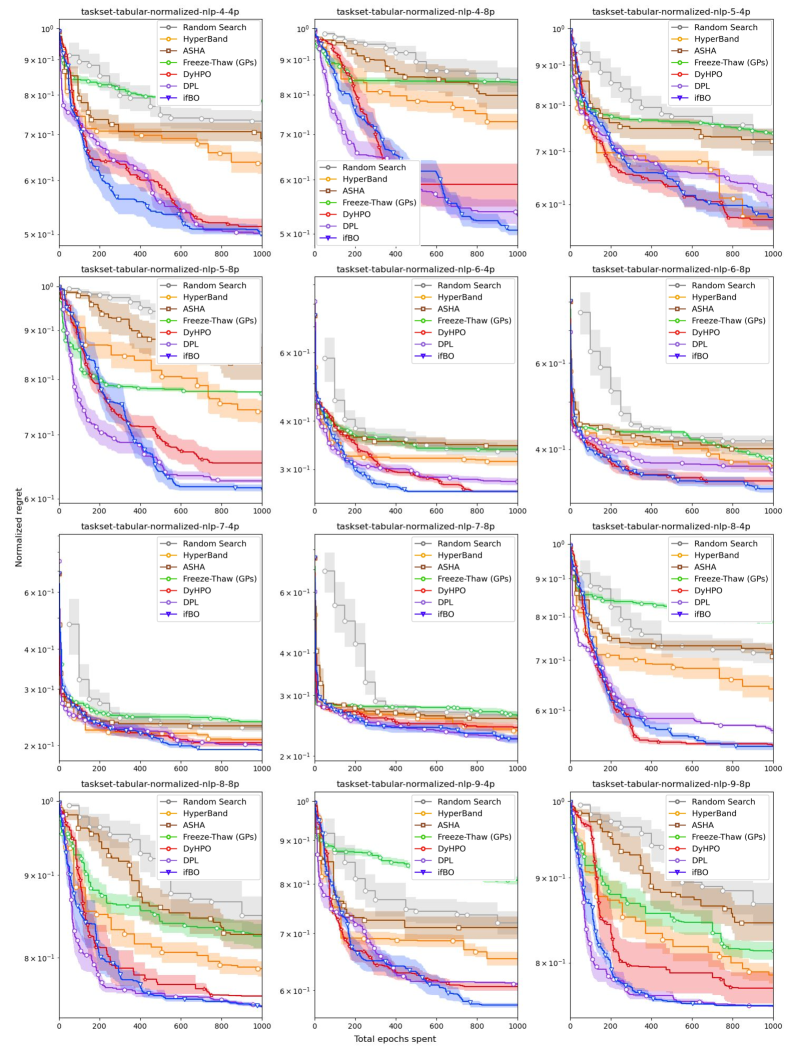
Figure 16: Per-task HPO results on Taskset (cont.)

References

- Adriaensen et al. (2023) Adriaensen, S., Rakotoarison, H., Müller, S., and Hutter, F. Efficient bayesian learning curve extrapolation using prior-data fitted networks. In Proceedings of the 37th International Conference on Advances in Neural Information Processing Systems (NeurIPS’23), 2023.
- Awad et al. (2021) Awad, N., Mallik, N., and Hutter, F. DEHB: Evolutionary hyberband for scalable, robust and efficient Hyperparameter Optimization. In Zhou, Z. (ed.), Proceedings of the 30th International Joint Conference on Artificial Intelligence (IJCAI’21), 2021.
- Bischl et al. (2023) Bischl, B., Binder, M., Lang, M., Pielok, T., Richter, J., Coors, S., Thomas, J., Ullmann, T., Becker, M., Boulesteix, A., Deng, D., and Lindauer, M. Hyperparameter optimization: Foundations, algorithms, best practices, and open challenges. 2023.
- Bojar et al. (2015) Bojar, O., Chatterjee, R., Federmann, C., Haddow, B., Huck, M., Hokamp, C., Koehn, P., Logacheva, V., Monz, C., Negri, M., Post, M., Scarton, C., Specia, L., and Turchi, M. Findings of the 2015 workshop on statistical machine translation. In Proceedings of the Tenth Workshop on Statistical Machine Translation, Lisbon, Portugal, September 2015.
- Caballero et al. (2023) Caballero, E., Gupta, K., Rish, I., and Krueger, D. Broken neural scaling laws. In International Conference on Learning Representations (ICLR’23), 2023.
- Chandrashekaran & Lane (2017) Chandrashekaran, A. and Lane, I. R. Speeding up hyper-parameter optimization by extrapolation of learning curves using previous builds. In Joint European Conference on Machine Learning and Knowledge Discovery in Databases. Springer, 2017.
- Chelba et al. (2013) Chelba, C., Mikolov, T., Schuster, M., Ge, Q., Brants, T., and Koehn, P. One billion word benchmark for measuring progress in statistical language modeling. arXiv preprint arXiv:1312.3005, 2013.
- Chen et al. (2022) Chen, Y., Song, X., Lee, C., Wang, Z., Zhang, Q., Dohan, D., Kawakami, K., Kochanski, G., Doucet, A., Ranzato, M., Perel, S., and de Freitas, N. Towards learning universal hyperparameter optimizers with transformers. In Koyejo, S., Mohamed, S., Agarwal, A., Belgrave, D., Cho, K., and Oh, A. (eds.), Proceedings of the 36th International Conference on Advances in Neural Information Processing Systems (NeurIPS’22), 2022.
- Deng (2012) Deng, L. The mnist database of handwritten digit images for machine learning research. IEEE Signal Processing Magazine, 29(6):141–142, 2012.
- Domhan et al. (2015) Domhan, T., Springenberg, J., and Hutter, F. Speeding up automatic Hyperparameter Optimization of deep neural networks by extrapolation of learning curves. In Yang, Q. and Wooldridge, M. (eds.), Proceedings of the 24th International Joint Conference on Artificial Intelligence (IJCAI’15), 2015.
- Dooley et al. (2023) Dooley, S., Khurana, G. S., Mohapatra, C., Naidu, S., and White, C. ForecastPFN: Synthetically-trained zero-shot forecasting. In Proceedings of the 37th International Conference on Advances in Neural Information Processing Systems (NeurIPS’23), 2023.
- Falkner et al. (2018) Falkner, S., Klein, A., and Hutter, F. BOHB: Robust and efficient Hyperparameter Optimization at scale. In Dy, J. and Krause, A. (eds.), Proceedings of the 35th International Conference on Machine Learning (ICML’18), volume 80. Proceedings of Machine Learning Research, 2018.
- Feurer & Hutter (2019) Feurer, M. and Hutter, F. Hyperparameter Optimization. In Hutter, F., Kotthoff, L., and Vanschoren, J. (eds.), Automated Machine Learning: Methods, Systems, Challenges, chapter 1, . Springer, 2019.
- Gargiani et al. (2019) Gargiani, M., Klein, A., Falkner, S., and Hutter, F. Probabilistic rollouts for learning curve extrapolation across hyperparameter settings. In 6th ICML Workshop on Automated Machine Learning, 2019.
- Gijsbers et al. (2019) Gijsbers, P., LeDell, E., Poirier, S., Thomas, J., Bischl, B., and Vanschoren, J. An open source automl benchmark. In Eggensperger, K., Feurer, M., Hutter, F., and Vanschoren, J. (eds.), ICML workshop on Automated Machine Learning (AutoML workshop 2019), 2019.
- Gilmer et al. (2021) Gilmer, J. M., Dahl, G. E., and Nado, Z. init2winit: a jax codebase for initialization, optimization, and tuning research, 2021.
- He et al. (2016) He, K., Zhang, X., Ren, S., and Sun, J. Deep residual learning for image recognition. In Proceedings of the International Conference on Computer Vision and Pattern Recognition (CVPR’16), 2016.
- Hollmann et al. (2023) Hollmann, N., Müller, S., Eggensperger, K., and Hutter, F. TabPFN: A transformer that solves small tabular classification problems in a second. In International Conference on Learning Representations (ICLR’23), 2023.
- Kadra et al. (2023) Kadra, A., Janowski, M., Wistuba, M., and Grabocka, J. Deep power laws for hyperparameter optimization. In Proceedings of the 37th International Conference on Advances in Neural Information Processing Systems (NeurIPS’23), 2023.
- Kingma et al. (2015) Kingma, D., Salimans, T., and Welling, M. Variational dropout and the local reparameterization trick. In Cortes, C., Lawrence, N., Lee, D., Sugiyama, M., and Garnett, R. (eds.), Proceedings of the 29th International Conference on Advances in Neural Information Processing Systems (NeurIPS’15), 2015.
- Klein et al. (2017) Klein, A., Falkner, S., Springenberg, J., and Hutter, F. Learning curve prediction with Bayesian neural networks. In Proceedings of the International Conference on Learning Representations (ICLR’17), 2017.
- Klein et al. (2020) Klein, A., Tiao, L., Lienart, T., Archambeau, C., and Seeger, M. Model-based Asynchronous Hyperparameter and Neural Architecture Search. arXiv:2003.10865 [cs.LG], 2020.
- Krizhevsky (2009) Krizhevsky, A. Learning multiple layers of features from tiny images. Technical report, University of Toronto, 2009.
- Lefaudeux et al. (2022) Lefaudeux, B., Massa, B., Liskovich, D., Xiong, W., Caggiano, W., Naren, S., Xu, M., Hu, J., Tintore, M., Zhang, S., Labatut, P., and Haziza, D. xformers: A modular and hackable transformer modelling library, 2022.
- Li et al. (2020a) Li, J., Liu, Y., Liu, J., and Wang, W. Neural architecture optimization with graph VAE. arXiv:2006.10310 [cs.LG], 2020a.
- Li et al. (2017) Li, L., Jamieson, K., DeSalvo, G., Rostamizadeh, A., and Talwalkar, A. Hyperband: Bandit-based configuration evaluation for Hyperparameter Optimization. In Proceedings of the International Conference on Learning Representations (ICLR’17), 2017.
- Li et al. (2020b) Li, L., Jamieson, K., Rostamizadeh, A., Gonina, E., Ben-tzur, J., Hardt, M., Recht, B., and Talwalkar, A. A system for massively parallel hyperparameter tuning. In Dhillon, I., Papailiopoulos, D., and Sze, V. (eds.), Proceedings of Machine Learning and Systems 2, volume 2, 2020b.
- Liao & Carneiro (2022) Liao, Z. and Carneiro, G. Competitive multi-scale convolution. arXiv preprint arXiv:1511.05635, 2022.
- Loshchilov & Hutter (2017) Loshchilov, I. and Hutter, F. SGDR: Stochastic gradient descent with warm restarts. In Proceedings of the International Conference on Learning Representations (ICLR’17), 2017.
- Mallik et al. (2023) Mallik, N., Bergman, E., Hvarfner, C., Stoll, D., Janowski, M., Lindauer, M., Nardi, L., and Hutter, F. Priorband: Practical hyperparameter optimization in the age of deep learning. In Thirty-seventh Conference on Neural Information Processing Systems, 2023.
- Metz et al. (2020) Metz, L., Maheswaranathan, N., Sun, R., Freeman, C. D., Poole, B., and Sohl-Dickstein, J. Using a thousand optimization tasks to learn hyperparameter search strategies. arXiv:2002.11887 [cs.LG], abs/, 2020.
- Mockus et al. (1978) Mockus, J., Tiesis, V., and Zilinskas, A. The application of Bayesian methods for seeking the extremum. Towards Global Optimization, 2(117-129), 1978.
- Müller et al. (2022) Müller, S., Hollmann, N., Arango, S., Grabocka, J., and Hutter, F. Transformers can do Bayesian inference. In Proceedings of the International Conference on Learning Representations (ICLR’22), 2022.
- Müller et al. (2023) Müller, S., Feurer, M., Hollmann, N., and Hutter, F. Pfns4bo: In-context learning for bayesian optimization. In Krause, A., Brunskill, E., Cho, K., Engelhardt, B., Sabato, S., and Scarlett, J. (eds.), Proceedings of the 40th International Conference on Machine Learning (ICML’23), volume 202 of Proceedings of Machine Learning Research. PMLR, 2023.
- Radford et al. (2019) Radford, A., Wu, J., Child, R., Luan, D., Amodei, D., and Sutskever, I. Language models are unsupervised multitask learners. OpenAI blog, 1(8):9, 2019.
- Ruhkopf et al. (2022) Ruhkopf, T., Mohan, A., Deng, D., Tornede, A., Hutter, F., and Lindauer, M. Masif: Meta-learned algorithm selection using implicit fidelity information. Transactions on Machine Learning Research, 2022.
- Russakovsky et al. (2015) Russakovsky, O., Deng, J., Su, H., Krause, J., Satheesh, S., Ma, S., Huang, Z., Karpathy, A., Khosla, A., Bernstein, M., Berg, A., and Fei-Fei, L. Imagenet large scale visual recognition challenge. 115(3):211–252, 2015.
- Swersky et al. (2014) Swersky, K., Snoek, J., and Adams, R. Freeze-thaw Bayesian optimization. arXiv:1406.3896 [stats.ML], 2014.
- Vaswani et al. (2017) Vaswani, A., Shazeer, N., Parmar, N., Uszkoreit, J., Jones, L., Gomez, A., Kaiser, L., and Polosukhin, I. Attention is all you need. In Guyon, I., von Luxburg, U., Bengio, S., Wallach, H., Fergus, R., Vishwanathan, S., and Garnett, R. (eds.), Proceedings of the 31st International Conference on Advances in Neural Information Processing Systems (NeurIPS’17). Curran Associates, Inc., 2017.
- Wang et al. (2021) Wang, Z., Dahl, G., Swersky, K., Lee, C., Mariet, Z., Nado, Z., Gilmer, J., Snoek, J., and Ghahramani, Z. Pre-trained Gaussian processes for Bayesian optimization. arXiv:2207.03084v4 [cs.LG], 2021.
- Wistuba et al. (2022) Wistuba, M., Kadra, A., and Grabocka, J. Dynamic and efficient gray-box hyperparameter optimization for deep learning. In Koyejo, S., Mohamed, S., Agarwal, A., Belgrave, D., Cho, K., and Oh, A. (eds.), Proceedings of the 36th International Conference on Advances in Neural Information Processing Systems (NeurIPS’22), 2022.
- Xiao et al. (2017) Xiao, H., Rasul, K., and Vollgraf, R. Fashion-MNIST: a novel image dataset for benchmarking Machine Learning algorithms. arXiv:1708.07747v2 [cs.LG], 2017.
- Zagoruyko & Komodakis (2016) Zagoruyko, S. and Komodakis, N. Wide residual networks. In Richard C. Wilson, E. R. H. and Smith, W. A. P. (eds.), Proceedings of the 27th British Machine Vision Conference (BMVC). BMVA Press, 2016.
- Zimmer et al. (2021) Zimmer, L., Lindauer, M., and Hutter, F. Auto-Pytorch: Multi-fidelity metalearning for efficient and robust AutoDL. 43:3079–3090, 2021.