A Communication- and Memory-Aware Model
for Load Balancing Tasks

Abstract

While load balancing in distributed-memory computing has been well-studied, we present an innovative approach to this problem: a unified, reduced-order model that combines three key components to describe “work” in a distributed system: computation, communication, and memory. Our model enables an optimizer to explore complex tradeoffs in task placement, such as increased parallelism at the expense of data replication, which increases memory usage. We propose a fully distributed, heuristic-based load balancing optimization algorithm, and demonstrate that it quickly finds close-to-optimal solutions. We formalize the complex optimization problem as a mixed-integer linear program, and compare it to our strategy. Finally, we show that when applied to an electromagnetics code, our approach obtains up to 2.3x speedups for the imbalanced execution.

I Introduction

As Moore’s law has arguably ended and the exascale era emerges, scientific applications are expected to run at larger scales to decrease time-to-solution. However, distributed-memory architectures have become more challenging to program efficiently. Achieving optimal performance often requires careful coordination and mapping of data along with computational work to the available hardware resources. Developers are often forced to make difficult decisions in trading off parallelism for communication, data replication, and memory use that may not be portable across different platforms. Task-based programming models have emerged as a possible solution, especially for irregular computational structures where manual work partitioning is particularly challenging. Instead of decomposing a problem to a fixed number of MPI ranks at startup, the programmer exposes concurrency to a middleware runtime system in the form of migratable tasks that can execute on different and possibly heterogeneous compute nodes.

Task-based paradigms vary greatly on the level and detail of information passed to the middleware, and the user is still often expected to make good decisions in breaking down work into tasks to get optimal performance. However, for a tasking model to be performance portable, where each task should run to get optimal performance (i.e., load balancing) is a key problem that should be passed to the middleware. For load balancing to be automated by the middleware, the profile of tasks must be predictable to some extent, or an online balancing scheme (e.g., work stealing) must be used. Although making online schemes locality-aware has been studied (cf. §II), these approaches still have many limitations in achieving optimal performance, especially under tight memory constraints.

This article thus makes the fundamental assumption that task profiles can be predicted by using a cost model. We use these predictions to propose a novel work model, called CCM (Computation Communication Memory), to describe the amount of work that each processor is performing under a task-to-processor mapping. Its primary contributions include:

• formulating the load balancing problem into a model that can be used to trade-off communication, processor load, and data replication under memory constraints;

• a fully distributed load balancing algorithm (called CCM-LB) that uses the CCM model to redistribute tasks;

• a recasting as a mixed-integer linear program (MILP) of the CCM optimization problem, to validate that CCM-LB finds solutions at worst 1.8% slower than optimal ones;

• a machine learning approach for the non-iterative (i.e., without repetitive behaviour across iterations) target application to predict task durations fed into CCM-LB; and,

• an application of our approach to an electromagnetics code, demonstrating a 2.3x speedup for the imbalanced matrix assembly on 128 nodes.

II Related Work

Load balancing is a well-known and extensively studied problem. Regularly-structured applications often achieve load balance through data distribution and careful orchestration of communication (e.g., multipartitioning [1]). For subclasses of regularly-structured computations (e.g., affine loops), extensive research has studied the memory and communication tradeoffs for generating distributed-memory mappings [2, 3]. This has been extended to broader classes such as tensor computations [4]. Inspector-executor approaches can often apply to calculations involving sparse matrices [5] or meshes [6] where computational data and load can be analyzed a priori at runtime before it starts (e.g., CHAOS [7]). Partitioning schemes [8], whose parallelization [9, 10, 11] is non-trivial, are often applied in this context. However, the data replication within memory constraints, which graph partitioners typically do not consider, must be explored for our target application.

Online dynamic load balancing approaches such as Cilk’s work stealing [12] are widely studied, with provably optimal space and time bounds for uniform shared-memory machines on fully-strict parallelism. Such schedulers have been extended for distributed memory [13], but ignore data locality and memory limits. Subsequent work in shared-memory has extended work stealing to be more aware of data locality, such as in hierarchical place trees [14] and similar approaches [15].

Task mapping has been studied for dataflow runtimes (e.g., PaRSEC [16], StarPU [17], Legion [18]), but often requires the user to generate an efficient mapping. To express an application with dataflow often requires a complete rewrite with data use types exposed (which is impractical for many real applications), and exposes many degrees of freedom to explore. Recent work [19] has shown that automated mappers may be feasible but difficult to scale. A MILP-based approach for mapping tasks to hardware is given by [20], but the description is terse and it is not immediately clear how the Boolean constraints are converted into integer ones, which is necessary if they are to be resolved by a MILP solver.

For iterative applications, scalable persistence-based load balancers that are hierarchical [21] or distributed [22] may be applied. However, these strategies often do not consider communication and lack the ability to consider data replication and memory constraints.

Various parallel computation models [23] have been proposed to model the costs of executing a parallel program on hardware, such as PRAM [24] and LogP [25]. These models are in the same vein as our proposed model, CCM.

II-A Background & Challenges

In this article, we devise and build a novel work model combining three elements: (1) computation (time spent executing a task), (2) communication between tasks, and (3) memory utilized by tasks (including shared memory). The complex interplay between these elements creates an combinatorially large search space for finding the optimal task assignments across nodes. Furthermore, we propose a scalable algorithm to efficiently search this space in an incremental manner, so task assignments can be refined over time. Such a tunable algorithm should allow users to trade off quality with time complexity, and thus lower the cost of running the load balancer.

The goal of a load balancer is to minimize the total time an application spends working. A corollary to this is minimizing the longest time any rank spends working. Thus, a load balancer may try to reduce the highest rank load, $\max{\mathcal{L}}$, to be as close as possible to the population mean of loads across all ranks, $\mu_{\mathcal{L}}$. A simple statistic to assess load imbalance is $\mathcal{I}_{\mathcal{L}}:=\nicefrac{{\max{\mathcal{L}}}}{{\mu_{\mathcal{L}}}}-1$, vanishing if and only if all ranks have the same load, so none of them slow down the rest. However, while minimizing imbalance is necessary to obtain an optimal configuration, it is not sufficient if the total amount of work can vary. For instance, displacing tasks from one rank to another may result in more overall communication across slower off-node network edges, thereby increasing total work and resulting in a longer execution time. Thus, a load balancing algorithm must rather minimize the total work across all ranks while also minimizing the maximum work performed on any rank.

The scalability of an application is further limited by the scalability of the load balancer itself. For large scales, fully distributed load balancing schemes show the most promise. However, the quality of the distributions produced and the complexity of implementation have traditionally limited their efficacy in practice. Of particular interest to us have been fully-distributed epidemic (or gossip) algorithms, that distribute information across the ranks to be rebalanced, in a manner similar to that of an infectious disease spreading through a biological population. This approach has shown promise in an array of distributed applications, ranging from routing protocols [26] to database consistency [27]. By building on original gossip-based work by Menon, et al. [22], we propose a novel distributed load balancing algorithm that optimizes task placement to minimize work while operating under strict memory constraints.

III Definitions & Models

We start by specifying terminology whose meaning varies throughout the literature, before introducing new concepts and mathematical formulations of importance to our approach.

III-A Parallel Model

III-A1 Nodes & Ranks

A node is the smallest compute unit connected to the network. A rank is a distinct process with a dedicated set of resources (e.g., CPU cores, GPUs) belonging to a node. The set of all ranks in the computation is denoted $R$.

III-A2 Phases

This paper focuses on load balancing a phase: a set of tasks across ranks that are to be executed between two synchronization points. For some scientific applications, a phase may be an iteration or timestep that evolves over time. For others, it may be the entire application’s execution. The proposed approach assumes that the tasks and communications are known or at least can be predicted (either by modeling, persistence, or an inspector-executor approach).

III-A3 Tasks

We define a task as a potentially multi-threaded, non-preemptable sequence of instructions that has a set of inputs and outputs, which include communications. Each task has an associated context in which it executes, consuming memory, and it may produce outputs that can subsequently spawn other tasks in other contexts. The set of tasks present during a phase $p$ is denoted ${T^{p}}$ and the set of tasks on rank $r$ during phase $p$ is denoted ${T_{r}^{p}}$.

III-A4 Shared memory blocks

These are memory chunks accessed by multiple tasks, to either read them or perform commutative and associative update operations on them. A shared block $s$ has a set of tasks ${T_{s}^{p}}$ accessing it, and it may be replicated across ranks to increase parallelism at the cost of higher communication and memory use. Each task $t$ is thus associated with a set of shared blocks ${S_{t}^{p}}$; each rank $r$ is associated with ${S_{r}^{p}}$$:=$$\cup_{t\in{T_{r}^{p}}}{S_{t}^{p}}$; and, ${S^{p}}$$:=$$\cup_{r\in{R}}{S_{r}^{p}}$ is the set of all shared blocks. To limit complexity, we assume that each task accesses at most one shared block, so that ${S_{t}^{p}}$ is either $\varnothing$ or a singleton.

III-B Compute Model

A compute model is an abstraction that predicts the required time (in $\text{\,}\mathrm{s}$) to complete the computations contained in task $t$ at phase $p$, denoted ${{\mathcal{L}}^{p}(t)}$. Denoting ${T_{r}^{p}}$ the set of tasks present on rank $r$ at phase $p$, the load of $r$ is readily computed as:

$${{\mathcal{L}}^{p}(r)}:=\textstyle\sum_{t\in{T_{r}^{p}}}{{\mathcal{L}}^{p}(t)}.$$ (1)

Evidently, it is not necessary to recompute rank loads using (1) when transferring a task $t$ from a rank $r_{1}$ to another rank $r_{2}$; the following update formulæ can be used instead:

$${{\widetilde{{\mathcal{L}}}}^{p}(r_{1})}={{\mathcal{L}}^{p}(r_{1})}-{{\mathcal{L}}^{p}(t)},\quad{{\widetilde{{\mathcal{L}}}}^{p}(r_{2})}={{\mathcal{L}}^{p}(r_{2})}+{{\mathcal{L}}^{p}(t)}.$$ (2)

III-C Communication Model

The set of input and output communications of a task $t$ at phase $p$ are respectively denoted ${\accentset{{\leftarrow}}{{C_{t}^{p}}}}$ and ${\accentset{{\to}}{{C_{t}^{p}}}}$, and

$$C^{p}:=\bigcup_{\;r\in{}R^{\phantom{p}}_{\phantom{r}}}\!\bigcup_{t\in{T_{r}^{p}}}{\accentset{{\leftarrow}}{{C_{t}^{p}}}}=\bigcup_{\;r\in{}R^{\phantom{p}}_{\phantom{r}}}\!\bigcup_{t\in{T_{r}^{p}}}{\accentset{{\to}}{{C_{t}^{p}}}},$$ (3)

thanks to the symmetry between inter-task inputs and outputs. In other words, the across-rank, across-task union of sent communications is equal to that of received ones. The volume of communications sent from task $t_{1}$ and received by task $t_{2}$ during phase $p$ (measured in bytes ($\text{\,}\mathrm{B}$)) is denoted ${\mathcal{V}^{p}(t_{1},t_{2})}$. Inter-task communications are aggregated at the rank level, as

$${\mathcal{V}^{p}(r_{1},r_{2})}:=\textstyle\sum_{(t_{1},t_{2})\in{T_{r_{1}}^{p}}\times{T_{r_{2}}^{p}}}{\mathcal{V}^{p}(t_{1},t_{2})}.$$ (4)

In particular, ${{\mathcal{V}^{p}(r)}}:=$${\mathcal{V}^{p}(r,r)}$ is the total on-rank communication volume for $r$, whose time cost per byte is orders of magnitude smaller than off-rank time cost per byte, defined as:

$${{\mathcal{V}_{\scriptscriptstyle\notin}^{p}(r)}}:=\max\Biggl{(}\sum_{\hskip 14.00003ptr_{0}\in R\setminus\{r\}}{\mathcal{V}^{p}(r,r_{0})},\sum_{\hskip 14.00003ptr_{0}\in R\setminus\{r\}}{\mathcal{V}^{p}(r_{0},r)}\Biggr{)}.$$ (5)

III-D Memory Model

Each node has a fixed amount of random-access memory, and thus the load balancer must prescribe a feasible task redistribution, so as not to exceed this memory limit. Being mapped to a certain node, each rank $r$ thus partakes of this limit, for it has a baseline working memory usage ${{\mathcal{M}_{\scriptscriptstyle-}^{p}\!\left(r\right)}}$ measured at the start of phase $p$, including base process usage and application data structures. Moreover, each task $t$ itself has baseline memory usage ${{\mathcal{M}_{\scriptscriptstyle-}^{p}\!\left(t\right)}}$, always used, and overhead working memory ${{\mathcal{M}_{\scriptscriptstyle+}^{p}\!\left(t\right)}}$ during execution, neither of which includes memory for any shared blocks it might access. These task memory components are then assembled at the rank level:

$${{\mathcal{M}_{T}^{p}\!\left(r\right)}}:=\sum_{t\in{T_{r}^{p}}}\!{{\mathcal{M}_{\scriptscriptstyle-}^{p}\!\left(t\right)}}+\max_{t\in{T_{r}^{p}}}{{\mathcal{M}_{\scriptscriptstyle+}^{p}\!\left(t\right)}}.$$ (6)

Furthermore, each shared block $s$ has a maximum amount of working memory it may consume during phase $p$, denoted ${{\mathcal{M}^{p}\!\left(s\right)}}$. The size of the shared blocks operated on $r$ is thus ${{\mathcal{M}_{S}^{p}\!\left(r\right)}}:=\sum_{s\in{S_{r}^{p}}}\!{{\mathcal{M}^{p}\!\left(s\right)}}$. The maximum memory usage combines the baseline, task, and shared memory components:

$${{\mathcal{M}_{\mathrm{\max}}^{p}\!\left(r\right)}}:={{\mathcal{M}_{\scriptscriptstyle-}^{p}\!\left(r\right)}}+{{\mathcal{M}_{T}^{p}\!\left(r\right)}}+{{\mathcal{M}_{S}^{p}\!\left(r\right)}}.$$ (7)

Consequently, if ${{\mathcal{M}_{\scriptscriptstyle\infty}\!\left(\mathfrak{n}\right)}}$ is the available memory on a given node $\mathfrak{n}$, i.e., the upper limit on the combined memory usage for all ranks on $\mathfrak{n}$, the following constraint must hold:

$$\sum_{r\in\mathfrak{n}}{{\mathcal{M}_{\mathrm{\max}}^{p}\!\left(r\right)}}\leq{{\mathcal{M}_{\scriptscriptstyle\infty}\!\left(\mathfrak{n}\right)}}.$$ (8)

To further reduce complexity, we apply the more stringent per-rank memory condition:

$$(\forall{}r\!\in\mathfrak{n})\enskip{{\mathcal{M}_{\mathrm{\max}}^{p}\!\left(r\right)}}\leq{{\mathcal{M}_{\scriptscriptstyle\infty}\!\left(r\right)}}:=\tfrac{1}{|\{r_{0}\in\mathfrak{n}\}|}{{\mathcal{M}_{\scriptscriptstyle\infty}\!\left(\mathfrak{n}\right)}},$$ (9)

which is evidently sufficient for (8), but not necessary to it.

The home of a shared block that will be read by tasks is the rank on which it is initialized. For shared blocks that are being updated, however, the home is uniquely defined as the rank on which the fully computed shared block will be consumed in a subsequent phase, which is typically the rank on which the tasks that update it were initialized. The set of all shared blocks homed at rank $r$ for phase $p$ is denoted ${\widehat{S}_{r}^{p}}$. A shared block requires extra communication when computed on or read from any rank other than its home, a cost which in our model is imputed to the rank with the off-home shared block, as:

$${{\mathcal{M}_{H}^{p}\!\left(r\right)}}:=\textstyle\sum_{s\in{S_{r}^{p}}\setminus{\widehat{S}_{r}^{p}}}{{\mathcal{M}^{p}\!\left(s\right)}}.$$ (10)

In a manner similar to what we did for load in (2), we derive update formulæ for homing costs, when a task $t\in{T_{r_{1}}^{p}}$ is transferred from a rank $r_{1}$ to another rank $r_{2}$, resulting in new shared block sets ${{\widetilde{S}}_{r_{1}}^{p}}$ and ${{\widetilde{S}}_{r_{2}}^{p}}$:

Theorem III.1 (Homing communications update formulæ).

$${{{\widetilde{\mathcal{M}}}_{H}^{p}(r_{1})}} ={{\mathcal{M}_{H}^{p}\!\left(r_{1}\right)}}-\textstyle\sum_{s\in({S_{t}^{p}}\setminus{{\widetilde{S}}_{r_{1}}^{p}})\setminus{\widehat{S}_{r_{1}}^{p}}}{{\mathcal{M}^{p}\!\left(s\right)}},$$ (11)

$${{{\widetilde{\mathcal{M}}}_{H}^{p}(r_{2})}} ={{\mathcal{M}_{H}^{p}\!\left(r_{2}\right)}}+\textstyle\sum_{s\in({S_{t}^{p}}\setminus{S_{r_{2}}^{p}})\setminus{\widehat{S}_{r_{2}}^{p}}}{{\mathcal{M}^{p}\!\left(s\right)}}.$$ (12)

Proof.

Omitted for brevity, refer to Appendix A. ∎

III-E CCM Model

Our proposed CCM model incorporates all components defined separately above in (1), (4), (5), and (10), and the memory constraint (9) in the form of a possibly-infinite penalization term, within the following quasi-affine combination:

$${{\mathcal{W}^{p}}(r)}:=\alpha{{\mathcal{L}}^{p}(r)}+\beta{{\mathcal{V}_{\scriptscriptstyle\notin}^{p}(r)}}+\gamma{{\mathcal{V}^{p}(r)}}+\delta{{\mathcal{M}_{H}^{p}\!\left(r\right)}}+\varepsilon,$$ (13)

with the following coefficients:

coefficient	unit	support	description
$\alpha$	$\varnothing$	${\mathbb{Z}_{2}}$	exclusion/inclusion of (1)
$\beta,\gamma$	$\text{\,}\mathrm{s}\mathrm{/}\mathrm{B}$	${\mathbb{R}_{\scriptscriptstyle+}}$	scales (4) & (5) to time
$\delta$	$\text{\,}\mathrm{s}\mathrm{/}\mathrm{B}$	${\mathbb{R}_{\scriptscriptstyle+}}$	scales (10) to time
$\varepsilon$	$\text{\,}\mathrm{s}$	$\{0;+\infty\}$	0 if (9) holds, else $+\infty$

The scaling coefficients $\beta$, $\gamma$, and $\delta$ may be measured empirically on a per-system basis, or evaluated from first principles.

In order to update the $\beta$ and $\gamma$ terms in the work model, the intra- and inter-rank communication must also be updated. This is done by finding edges that change from local to remote when a task is transferred between ranks. For brevity, the update formulæ are not presented here, but can be derived from equations (4), and (5).

IV Distributed & Constrained Load Balancing

We now present our distributed algorithm, CCM-LB, which iteratively optimizes task placement to reduce overall work as computed by the CCM model. First, each iteration builds a distributed peer network for each rank by propagating rank-local information. Second, ranks can attempt to transfer work within their known peer set, by evaluating a criterion using only locally-known information.

⬇

1info_known = dict() /* rank-local peer network info */

2

3def ComputeCCM(rank, add_tasks = [], remove_tasks = []):

4 /* apply update formulae to compute new work with add_tasks added and remove_tasks removed from rank */

5

6def FindBestCCM(rank, peer):

7 best_work_diff = -inf

8 work_r, work_p = ComputeCCM(rank), ComputeCCM(peer)

9 max_work = max(work_r, work_p)

10 for c_r in getClusters(rank):

11 for c_p in getClusters(peer):

12 work_r_after = ComputeCCM(rank, c_p, c_r)

13 work_p_after = ComputeCCM(peer, c_r, c_p)

14 max_work_after = max(work_r_after, work_p_after)

15 work_diff = max_work - max_work_after

16 if work_diff > 0:

17 best_work_diff = max(best_work_diff, work_diff)

18 return best_work_diff

19

20def TryTransfer(rank, peer):

21 best_work_diff = FindBestCCM(rank, peer)

22 if best_work_diff > 0:

23 /* perform task transfers for best_work_diff */

24

25def BuildPeerNetwork(k_rounds, fanout):

26 info_known.clear()

27 info_known[rank] = /*information from this rank*/

28 def spreadInfo(cur_round, new_info):

29 info_known[a] = b for a,b in new_info

30 if cur_round < k_rounds:

31 for f in fanout:

32 p = /* generate random peer */

33 send(spreadInfo, @p, cur_round+1, info_known)

34 spreadInfo(1, nil)

35 return info_known.keys()

36

37def CCM_LB(n_iter, k_rounds, fanout, rank):

38 for i in n_iter:

39 peers = BuildPeerNetwork(k_rounds, fanout)

40 for p in peers:

41 work_list.append(FindBestCCM(rank,p),p)

42 for (work, peer) in sort(work_list):

43 has_lock = TryLock(peer)

44 if has_lock:

45 if IsLocked(rank) and GetLockingRank(rank) <= peer:

46 Unlock(peer)

47 work_list.append((work, peer))

48 else:

49 while IsLocked(rank): pass /* wait to be unlocked */

50 @when recvUpdate(peer_info):

51 info_known[peer] = peer_info /* update */

52 TryTransfer(rank, peer)

53 Unlock(peer)

Figure 1: The CCM-LB algorithm.

Before CCM-LB builds peer networks, we first generate clusters of tasks (on each rank) that are highly connected based on the weights of the CCM model. These clusters are generated based on tasks that communicate heavily or access the same shared memory block(s). Clusters are important to consider migrating together as splitting them apart often increases the amount of work in the system or increases memory usage (since the same shared block will be accessed by more ranks as they are split).

IV-A Augmented Inform Stage

During peer network building, each rank sends its local information to $f$ (the fanout) randomly selected peer ranks over a number of asynchronous rounds. When a message is received, its recipient augments it with its known information and, if the information round is less than the prescribed number of rounds, propagates it further to $f$ ranks not visited before by this message, as shown on line 30 of Figure 1.

In contrast to previous work [22], information beyond rank loads must be propagated, for without knowledge of the memory and communication on a given rank, another rank cannot evaluate whether tasks can be transferred even if it is underloaded. We thus augment the inform messages with on- and off-rank communication volumes (${{\mathcal{V}^{p}(r)}}$, ${{\mathcal{V}_{\scriptscriptstyle\notin}^{p}(r)}}$), homing cost ${{\mathcal{M}_{H}^{p}\!\left(r\right)}}$, baseline rank footprint memory ${{\mathcal{M}_{\scriptscriptstyle-}^{p}\!\left(r\right)}}$, and a summary of the clusters found on that rank $r$. For each cluster $c$, we send the load ${{\mathcal{L}}^{p}(c)}$, the sizes of the shared blocks accessed by the cluster ${S_{c}^{p}}$, the inter- and intra-cluster communication volumes (${{\mathcal{V}^{p}(c)}}$, ${{\mathcal{V}_{\scriptscriptstyle\notin}^{p}(c)}}$), and the cluster memory baseline footprint ${{\mathcal{M}_{\scriptscriptstyle-}^{p}\!\left(c\right)}}$. This additional data allows us to approximate the work model as we consider remapping tasks. We note that while the rank-based additions have constant size, the cluster-based component is $\mathcal{O}(|C|)$, where $C$ is the set of clusters, leading to an increased upper-bound on space during the inform stage.

IV-B Task Transfer Algorithm

In previous work [22], the transfer phase begins after peer network building by using a cumulative mass function to bias random selection of ranks for potential transfer depending on how underloaded they are. Then, work units are selected from the overloaded rank and given to the underloaded without any intervention. In further work, an underloaded rank was allowed to negatively acknowledge a requested transfer if it increases the load of this rank beyond the arithmetic mean of loads across all ranks.

In the landscape of the more complex criterion that includes (1) computation, (2) communication, and (3) memory as factors, it is infeasible for a rank to decide unilaterally to transfer tasks without full knowledge of the other rank’s tasks (including full communication information and memory requirements). Thus, the proposed algorithm operates in two stages. First, it applies the CCM update formulæ to decide how valuable transferring with a target rank might be (based on information that might be out-of-date). Second, it picks the most potentially viable rank to transfer work with and attempts to obtain a lock on that rank. Figure 1 provides an overview of the CCM-LB algorithm.

On line 39 of Figure 1, we build the random peer network for each rank, resulting in a list of ranks that each rank knows about. On line 41, each rank applies the criterion to each peer rank by calculating the amount of work (using the update formulæ) under possible task transfers. The best transfer (lowest resulting work) is put in a sorted list (work_list) for each peer. Each rank then tries to lock the peer that has the best potential transfer (line 43).

If all ranks are allowed to request and obtain a lock concurrently, deadlocks can easily occur. In the simplest case, ranks $r_{1}$ and $r_{2}$ might both send messages requesting a lock from each other. Rank $r_{1}$ may receive the request from $r_{2}$ and allow it to obtain a lock. Concurrently, rank $r_{2}$ may apply the same logic and allow $r_{1}$ to obtain a lock. By the time both ranks are notified, they may be locked and also hold a lock on the other rank. While a rank is locked it cannot make progress on a lock it holds because another rank might change its task distribution. These types of cycles can occur with an arbitrary number. To remediate this problem, if a rank $r_{1}$ is locked by another rank, $r_{x}$, and also obtains a lock on $r_{2}$, it immediately releases the lock if $r_{x}\leq r_{2}$ (shown on line 45). This logic guarantees that cycles will not form. The option to lock $r_{2}$ is added back to the work_list so it can try to obtain the lock later once it has been unlocked.

Once a lock succeeds, a message is sent from $r_{2}$ to $r_{1}$ with up-to-date information on the tasks residing on $r_{2}$. Once received, TryTransfer is invoked, calling FindBestCCM (line  21) to search for clusters that can be given or swapped to reduce the maximum work between the two ranks. It evaluates many such possible transfers and selects the best one to execute (if one exists that is better than the current configuration shown on line 16). After every rank has exhausted its list of possible ranks to transfer in work_list, and all selected transfers have occurred, the iteration is over. The algorithm proceeds with the next iteration by creating a new random peer network and performing the whole process again.

V Mixed-Integer Linear Programming Formulation

We now reformulate the task-rank problem assignment as a mixed-integer linear program (MILP), which is NP-hard. Our CCM model proposed in §III-E makes this formulation much more complex than a conventional job-machine assignment, due to the inclusion of additional components with assorted dependencies. We thus proceed in increasing order of complexity, from constrained compute-only to the full work model of (13).

V-A Common Definitions

We begin with notational conventions which, albeit not necessary, shall ease the understanding of our approach. For instance, summation indices are dummy and can be replaced without altering the meaning of the sum; but we believe it is more convenient to the reader if a given index letter always refers to the same type of entity:

entity type	set	cardinality	indices
ranks	$R$	$I$	$i,j$
tasks	${T^{p}}$	$K$	$k,\ell$
communications	$C^{p}$	$M$	$m$
shared blocks	${S^{p}}$	$N$	$n$

Subsequently, we define assignment matrices between the above defined entity types, using the indicator function:

to type	from type	size		matrix entries
tasks	shared blocks	$K$$\times$	$N$	$u^{p}_{k,n}$$:=$	$\mathds{1}_{S_{t_{k}}^{p}}(s_{n})$
ranks	shared blocks	$I$$\times$	$N$	$v^{p}_{i,n}$$:=$	$\mathds{1}_{\widehat{S}_{r_{i}}^{p}}(s_{n})$
ranks	shared blocks	$I$$\times$	$N$	$\phi^{p}_{i,n}$$:=$	$\mathds{1}_{S_{r_{i}}^{p}}(s_{n})$
ranks	tasks	$I$$\times$	$K$	$\chi^{p}_{i,k}$$:=$	$\mathds{1}_{T_{r_{i}}^{p}}(t_{k})$

Although $(v^{p})$ and $(\phi^{p})$ have the same shape, they differ in that the former specifies homing of a block to a rank, while the latter indicates the presence of the block on a rank. The problem statement does not allow the load balancer to modify either block-task or block-home assignments; as a result, both $(u^{p})$ and $(v^{p})$ are parameters, whereas both $(\phi^{p})$ and $(\chi^{p})$ are variables, whence the use of different alphabets to emphasize this contrast. Meanwhile, every task must be assigned to exactly one rank, and at most one shared block, while every block shall be homed at exactly one rank; therefore, the following $2K+N$ consistency constraints must hold:

$${\left(\forall{k}\in{\llbracket 1,{K}\rrbracket}\right)}\enskip \sum_{n=1}^{N}u^{p}_{k,n}\leq 1\enskip\land\enskip\sum_{i=1}^{I}\chi^{p}_{i,k}=1,$$ (14)

$${\left(\forall{n}\in{\llbracket 1,{N}\rrbracket}\right)}\enskip \sum_{i=1}^{I}v^{p}_{i,n}=1.$$ (15)

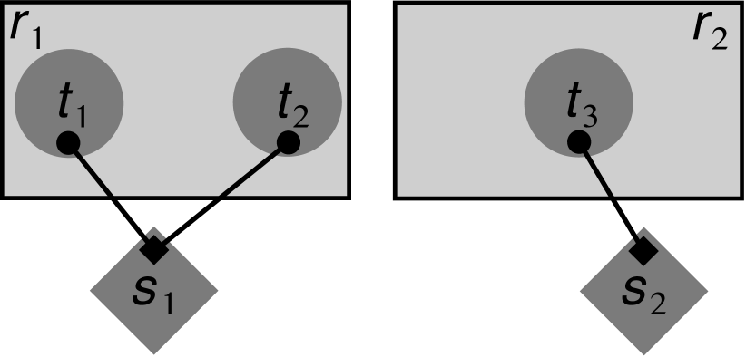
$\scriptstyle{T_{r_{1}}^{p}}=\{t_{1},t_{2}\}$ $\scriptstyle{T_{r_{2}}^{p}}=\{t_{3}\}$ $\scriptstyle\Rightarrow\enskip\scriptstyle(\chi^{p})=\left(\begin{smallmatrix}1&1&0\\ 0&0&1\end{smallmatrix}\right)$ $\begin{array}[]{@{}s@{}s@{}}{S_{t_{1}}^{p}}=\{s_{1}\}&{\hbox{\multirowsetup$\left.\rule{0.0pt}{20.0pt}\right\}{\!\scriptstyle(u^{p})=\left(\begin{smallmatrix}1&0\\ 1&0\\ 0&1\end{smallmatrix}\right)}$}}\\ {S_{t_{2}}^{p}}=\{s_{1}\}\\ {S_{t_{3}}^{p}}=\{s_{2}\}\end{array}$ $\begin{array}[]{@{}s@{\,}s@{\,}l@{}}(\phi^{p})&=&\scriptstyle\left(\begin{smallmatrix}1&1&0\\ 0&0&1\end{smallmatrix}\right)\odot\left(\begin{smallmatrix}1&0\\ 1&0\\ 0&1\end{smallmatrix}\right)\\ \hfil&=&\left(\begin{smallmatrix}1&0\\ 0&1\end{smallmatrix}\right)\hfill\\ \end{array}$

Figure 2: A Compute-Only Memory-Constrained Problem (COMCP) example for $I$$=$$2$, $K$$=$$3$, and $N$$=$$2$, with corresponding assignment sets and matrices.

As an illustrative example, consider an arrangement with $I$$=$$2$, $K$$=$$3$, and $N$$=$$2$, where the two first tasks are assigned to the first rank and share a memory block, while the remaining task is assigned to the second rank and is a lone participant in a second memory block, as shown in Figure 2. From this we obtain the assignment matrices, with both $(u^{p})$ and $(\chi^{p})$ satisfying the consistency constraints in (14). We further observe that, although $2^{6}$$=$$64$ different combinations of the $6$ binary entries in $(\chi^{p})$ may be formed, the consistency constraint eliminates $3$ degrees of freedom because the knowledge of, e.g., the first row unambiguously determines the second. There are, as expected, only $2^{3}$$=$$I^{K}$$=8$ consistent task-rank assignments.

Obviously, shared blocks do not roam freely between ranks; rather, their assignments are constrained by their associated tasks. Denoting $\odot$ the Boolean product between binary matrices, i.e., using the arithmetic of the $({\mathbb{Z}_{2}},\lor,\land)$ semiring, the fundamental constraint is:

Theorem V.1 (Boolean shared block matrix relations).

$$(\phi^{p})=(\chi^{p})\odot(u^{p}).$$ (16)

Proof.

Omitted for brevity, refer to Appendix A. ∎

Unfortunately, albeit elegant and tight, this property based on Boolean algebra does not lend itself to a linear program formulation. It must instead be re-cast in an integral, yet much less concise form, as follows:

Theorem V.2 (Integer shared block matrix relations).

$$\!(\forall k\!\in\!{\llbracket 1,{K}\rrbracket})\,\phi^{p}_{i,n}\geq u^{p}_{k,n}\chi^{p}_{i,k}$$ (17)

$$\phi^{p}_{i,n}\leq\sum_{k=1}^{K}u^{p}_{k,n}\chi^{p}_{i,k}.$$ (18)

Proof.

Omitted for brevity, refer to Appendix A. ∎

$~{}i$	$n$	$k$	$u^{p}_{k,n}$	$\chi^{p}_{i,k}$	$u^{p}_{k,n}\chi^{p}_{i,k}\leq$	$\phi^{p\vphantom{A}}_{i,n}$	$\leq\sum_{k}u^{p}_{k,n}\chi^{p}_{i,k}$
${1}\left\{\rule{0.0pt}{30.0pt}\right.$	${1}\left\{\rule{0.0pt}{15.0pt}\right.$	$1$	$1$	$1$	$\hfill{1}\hskip 14.0pt=$	$\left.\rule{0.0pt}{15.0pt}\right\}{1}$
		$2$	$1$	$1$	$\hfill{1}\hskip 14.0pt=$		$<\,\quad{2}\hfill$
		$3$	$0$	$0$	$\hfill{0}\hskip 14.0pt<$
	${2}\left\{\rule{0.0pt}{15.0pt}\right.$	$1$	$0$	$1$	$\hfill{0}\hskip 14.0pt=$	$\left.\rule{0.0pt}{15.0pt}\right\}{0}$
		$2$	$0$	$1$	$\hfill{0}\hskip 14.0pt=$		$=\,\quad{0}\hfill$
		$3$	$1$	$0$	$\hfill{0}\hskip 14.0pt=$
${2}\left\{\rule{0.0pt}{30.0pt}\right.$	${1}\left\{\rule{0.0pt}{15.0pt}\right.$	$1$	$1$	$0$	$\hfill{0}\hskip 14.0pt=$	$\left.\rule{0.0pt}{15.0pt}\right\}{0}$
		$2$	$1$	$0$	$\hfill{0}\hskip 14.0pt=$		$=\,\quad{0}\hfill$
		$3$	$0$	$1$	$\hfill{0}\hskip 14.0pt=$
	${2}\left\{\rule{0.0pt}{15.0pt}\right.$	$1$	$0$	$0$	$\hfill{0}\hskip 14.0pt<$	$\left.\rule{0.0pt}{15.0pt}\right\}{1}$
		$2$	$0$	$0$	$\hfill{0}\hskip 14.0pt<$		$=\,\quad{1}\hfill$
		$3$	$1$	$1$	$\hfill{1}\hskip 14.0pt=$

TABLE I: Compliance of assignment matrices to constraints (17) & (18).

We further remark that (17) provides tight bounds for all $K$ inequalities when $\phi_{i,n}$$=$$0$, and at least once when $\phi_{i,n}$$=$$1$. The latter can be established by contradiction: assuming strictness of all inequalities would imply that all $u^{p}_{k,n}\chi^{p}_{i,k}$ be nil, hereby causing $\phi_{i,n}$ to vanish as well and thus contradicting the hypothesis on $\phi_{i,n}$$=$$1$. In contrast, (18) does not provide a tight upper bound in general, as exhibited by Table I, which expounds the earlier illustrative example: for instance, $\phi_{1,1}$$=$$1$ but (18) only provides a loose upper bound thereof. However, because this may only occur when $\phi_{i,n}$$=$$1$, the problem is automatically remedied by the fact that the search space for $\phi_{i,n}$ is limited to ${\mathbb{Z}_{2}}$; in other words, another constraint (that of the definition domain) will compensate for the loose bound.

V-B Compute-Only Memory-Constrained Problem (COMCP)

The aim of this simplified model is to ensure that our approach works for compute-only load balancing under memory constraint, i.e., with $\alpha$$=$$1$ and $\beta$$=$$\gamma$$=$$\delta$$=$$0$ in (13). Regarding $\varepsilon$, the per-rank bound of (9) is used in combination with the definitions of $(\chi^{p})$ and $(\phi^{p})$ which, after replacing the $\max$ operator in (6) with $K$ linear inequalities, equivalently amounts to the following $I$$\times$$K$ constraints:

$$\!\!\!(\forall(i{,}k)\in{\llbracket 1,{I}\rrbracket}\!\times\!{\llbracket 1,{K}\rrbracket})\enskip\sum_{\ell=1}^{K}{{\mathcal{M}_{\scriptscriptstyle-}^{p}\!\left(t_{\ell}\right)}}\chi_{i,\ell}+{{\mathcal{M}_{\scriptscriptstyle+}^{p}\!\left(t_{k}\right)}}\chi_{i,k}\\ +\sum_{n=1}^{N}{{\mathcal{M}^{p}\!\left(s_{n}\right)}}\phi_{i,n}\leq{{\mathcal{M}_{\scriptscriptstyle\infty}\!\left(r_{i}\right)}}\!-\!{{\mathcal{M}_{\scriptscriptstyle-}^{p}\!\left(r_{i}\right)}}.$$ (19)

It might be tempting to view the decision variable as that obtained by vectorizing the $(\chi^{p})$ and $(\phi^{p})$ assignment matrices, followed by the concatenation of an $I(K$$+$$N)$-dimensional binary vector. However, this approach cannot be formulated in terms of a linear program because its objective function, $\max_{r\in{}R}{{\mathcal{W}^{p}}(r)}$, is not a linear combination of these binary variables. This difficulty can be resolved with the makespan formulation [28], which introduces an additional degree of freedom, in the form of a nonnegative continuous variable ${{\mathcal{W}_{\max}^{p}}}$ constraining ${{\mathcal{W}^{p}}(r)}$ from above. As work is reduced to the compute term in (13), this can be equivalently formulated in $I$ new constraints using task-rank assignments:

$${\left(\forall{i}\in{\llbracket 1,{I}\rrbracket}\right)}\enskip\sum_{k=1}^{K}{{\mathcal{L}}^{p}(t_{k})}\chi_{i,k}\leq{{\mathcal{W}_{\max}^{p}}}.$$ (20)

Forming the vector $\vec{x}^{p}$$=$$\mathrm{vec}\left(\overrightarrow{(\chi^{p})},\overrightarrow{(\phi^{p})},{{\mathcal{W}_{\max}^{p}}}\right)$ finally allows us to formulate the COMCP as the following MILP:

$$\operatorname*{arg\,min}_{\vec{x}^{p}\in{\mathbb{Z}_{2}}^{I(K\!+\!N)}\times{\mathbb{R}_{\scriptscriptstyle+}}}\quad \vec{c}\cdot\vec{x}^{p}$$ (21)

$$\mathrm{subject~{}to}\quad A\vec{x}^{p}=\vec{1}_{K}$$ (22)

$$\mathrm{subject~{}to}\quad B\vec{x}^{p}+\vec{b}\geq\vec{0}_{I(K\!+\!1)(N\!+\!1)}$$ (23)

where $\vec{c}$ has all nil entries, except for a final, unit coordinate corresponding to the ${{\mathcal{W}_{\max}^{p}}}$ entry in $\vec{x}^{p}$, so that $\vec{c}\cdot\vec{x}^{p}={{\mathcal{W}_{\max}^{p}}}$. Meanwhile, matrices $A$ (determined by the part of (14) concerning $(\chi^{p})$) and $B$, and vector $\vec{b}$ (determined by (17), (18), (19), and (20)) only contain input parameter values.

Continuing with the running example, $\vec{x}^{p}$ is $11$-dimensional and, e.g., using row-major vectorization and column-vector convention, $A=\left(\setcounter{MaxMatrixCols}{11}\begin{smallmatrix}1&0&0&1&0&0&0&0&0&0&0\\ 0&1&0&0&1&0&0&0&0&0&0\\ 0&0&1&0&0&1&0&0&0&0&0\end{smallmatrix}\right)$. For brevity, we only provide the main principles presiding to assembly of $B$, whose size is $24\times 11$: its first $16$ are directly given by the inequalities in Table I ($12$ and $4$ lower and upper bounds, respectively). Denoting parameters $d_{\ell}$$=$$-{{\mathcal{M}_{\scriptscriptstyle-}^{p}\!\left(t_{\ell}\right)}}$, $e_{k}$$=$$-{{\mathcal{M}_{\scriptscriptstyle+}^{p}\!\left(t_{k}\right)}}$, $f_{n}$$=$$-{{\mathcal{M}^{p}\!\left(s_{n}\right)}}$, and $g_{k}$$=$$-{{\mathcal{L}}^{p}(t_{k})}$ for conciseness, the last $6$$+$$2$$=$$8$ rows of $B$ are provided by (19) and (20) as follows:

$$\left(\setcounter{MaxMatrixCols}{11}\begin{smallmatrix}d_{1}+e_{1}&d_{2}&d_{3}&0&0&0&f_{1}&f_{2}&0&0&0\\ d_{1}&d_{2}+e_{2}&d_{3}&0&0&0&f_{1}&f_{2}&0&0&0\\ d_{1}&d_{2}&d_{3}+e_{3}&0&0&0&f_{1}&f_{2}&0&0&0\\ 0&0&0&d_{1}+e_{1}&d_{2}&d_{3}&0&0&f_{1}&f_{2}&0\\ 0&0&0&d_{1}&d_{2}+e_{2}&d_{3}&0&0&f_{1}&f_{2}&0\\ 0&0&0&d_{1}&d_{2}&d_{3}+e_{3}&0&0&f_{1}&f_{2}&0\\ g_{1}&g_{2}&g_{3}&0&0&0&0&0&0&0&1\\ 0&0&0&g_{1}&g_{2}&g_{3}&0&0&0&0&1\end{smallmatrix}\right).$$

Finally, all entries of $\vec{b}$ are nil, except those two corresponding to the opposite of the right-hand sides in (19).

V-C Full Work Model Problem (FWMP)

All terms in (13) are now retained. The framework introduced above for the COMCP is conserved; in particular:

• the minimization problem (21) remains essentially identical, but $\vec{x}^{p}$ is expanded to include the assignments of communications to ranks, while $\vec{c}$ is expanded by as many nil entries so that only ${{\mathcal{W}_{\max}^{p}}}$ will not be canceled;

• constraint (22) is kept unchanged, and so are the contributions to (23) of (17), (18), and (19).

However, the communication volumes and homing costs must be added to $B$ and $\vec{b}$. We thus introduce third-order assignment tensors, keeping our earlier Latin/Greek alphabetical convention for parameters vs. variables, respectively:

to type	from type	size			tensor entries
tasks	communications	$K$$\times$	$K$ $\times$	$M$	$w^{p}_{k,\ell,m}$$:=$	$\mathds{1}_{{\accentset{{\to}}{{C_{t_{k}}^{p}}}}\!\cap{\accentset{{\leftarrow}}{{C_{t_{\ell}}^{p}}}}}(c_{m})$
ranks	communications	$I$$\times$	$I$ $\times$	$M$	$\psi^{p}_{i,j,m}$$:=$	$\mathds{1}_{{\accentset{{\to}}{{C_{r_{i}}^{p}}}}\!\cap{\accentset{{\leftarrow}}{{C_{r_{j}}^{p}}}}}(c_{m})$

We note one peculiarity of these tensors: as a communication edge has only two endpoints, they have only one nonzero entry per $m$-slice. The results of Theorem V.1 are readily extended to the communication assignment tensors:

Theorem V.3 (Boolean communication tensor relations).

$${\left(\forall{m}\in{\llbracket 1,{M}\rrbracket}\right)}\enskip{({\psi}^{p}_{::{m}})}=(\chi^{p})\odot{({w}^{p}_{::{m}})}\odot{{(\chi^{p})}^{\intercal}}.$$ (24)

Proof.

Omitted for brevity, refer to Appendix A. ∎

$\,\scriptstyle{\accentset{{\to}}{{C_{t_{1}}^{p}}}}\!=\{c_{1},c_{4}\},\hfil{\accentset{{\to}}{{C_{t_{2}}^{p}}}}\!=\{c_{2}\},\hfil{\accentset{{\to}}{{C_{t_{3}}^{p}}}}\!=\{c_{3}\},\hfil{\accentset{{\leftarrow}}{{C_{t_{1}}^{p}}}}\!=\varnothing,\hfil{\accentset{{\leftarrow}}{{C_{t_{2}}^{p}}}}\!=\{c_{3},c_{4}\},\hfil{\accentset{{\leftarrow}}{{C_{t_{3}}^{p}}}}\!=\{c_{1},c_{2}\}$
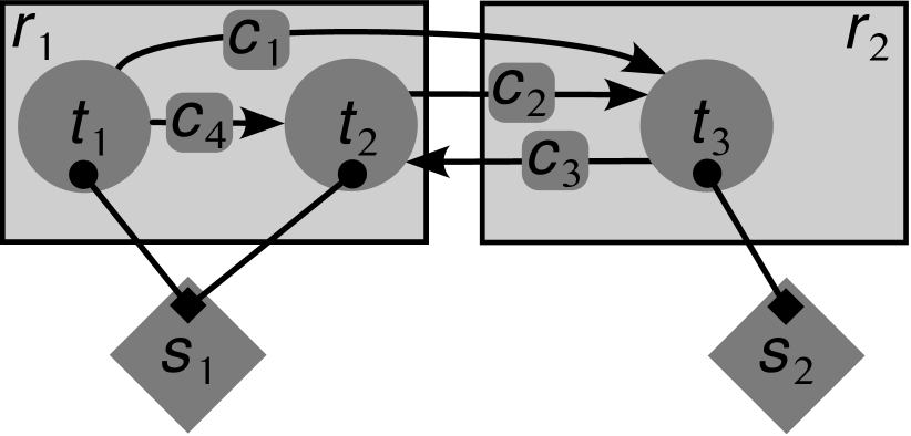
$\scriptstyle{\accentset{{\to}}{{C_{r_{1}}^{p}}}}\!=\{c_{1},c_{2},c_{4}\},\,{\accentset{{\to}}{{C_{r_{2}}^{p}}}}\!=\{c_{3}\},\,{\accentset{{\leftarrow}}{{C_{r_{1}}^{p}}}}\!=\{c_{3},c_{4}\},\,{\accentset{{\leftarrow}}{{C_{r_{2}}^{p}}}}\!=\{c_{1},c_{2}\}\,\Rightarrow$ $\scriptstyle\Rightarrow[w^{p}]$ $\overbrace{\hskip 390.25534pt}$ $\scriptscriptstyle{w}^{p}_{::{1}}$ $\scriptscriptstyle{w}^{p}_{::{2}}$ $\scriptscriptstyle{w}^{p}_{::{3}}$ $\scriptscriptstyle{w}^{p}_{::{4}}$ $\left[\!\begin{smallmatrix}0&0&0\\ 0&0&0\\ 1&0&0\end{smallmatrix}\!\middle|\!\begin{smallmatrix}0&0&0\\ 0&0&0\\ 0&1&0\end{smallmatrix}\!\middle|\!\begin{smallmatrix}0&0&0\\ 0&0&1\\ 0&0&0\end{smallmatrix}\!\middle|\!\begin{smallmatrix}0&0&0\\ 1&0&0\\ 0&0&0\end{smallmatrix}\!\right]$ $\scriptstyle(\chi^{p})\odot\;\Downarrow\;\odot{{(\chi^{p})}^{\intercal}}$ $\left[\begin{smallmatrix}0&0\\ 1&0\end{smallmatrix}\middle|\begin{smallmatrix}0&0\\ 1&0\end{smallmatrix}\middle|\begin{smallmatrix}0&1\\ 0&0\end{smallmatrix}\middle|\begin{smallmatrix}1&0\\ 0&0\end{smallmatrix}\right]$ $\scriptscriptstyle{\psi}^{p}_{::{1}}$ $\scriptscriptstyle{\psi}^{p}_{::{2}}$ $\scriptscriptstyle{\psi}^{p}_{::{3}}$ $\scriptscriptstyle{\psi}^{p}_{::{4}}$ $\underbrace{\hskip 303.53267pt}$ $\scriptstyle[\psi^{p}]$

Figure 3: A FWMP example for $I$$=$$2$, $K$$=$$3$, $M$$=$$4$, and $N$$=$$2$, with corresponding communication assignment sets and tensors.

By adding $M$$=$$4$ inter-task communications to the COMCP example of Figure 2, Theorem V.3 is illustrated in Figure 3. As done for the assignment matrices, the tensor constraints are reformulated in integral terms for the MILP framework:

Theorem V.4 (Integer communication tensor relations).

$$\psi_{i,j,m} \leq\sum_{\ell=1}^{L}\sum_{k=1}^{K}\chi_{i,k}w_{k,\ell,m},$$ (25)

$$\psi_{i,j,m} \leq\sum_{\ell=1}^{L}\sum_{k=1}^{K}\chi_{j,\ell}w_{k,\ell,m},$$ (26)

$$\psi_{i,j,m} \geq\sum_{\ell=1}^{L}\sum_{k=1}^{K}(\chi_{i,k}\!+\!\chi_{j,\ell})w_{k,\ell,m}\!-\!1.\!$$ (27)

Proof.

Omitted for brevity, refer to Appendix A. ∎

We illustrate Theorem V.4 with the example of Figure 3; first, (27) immediately sets the values of $\psi_{i,j,m}$ that are equal to $1$, as they cannot be greater by definition, as shown in bold:

$$\left[\begin{smallmatrix}0&{\!{\scriptscriptstyle-}1\!}\\ \mathbf{1}&0\end{smallmatrix}\middle|\begin{smallmatrix}0&{\!{\scriptscriptstyle-}1\!}\\ \mathbf{1}&0\end{smallmatrix}\middle|\begin{smallmatrix}0&\mathbf{1}\\ {\!{\scriptscriptstyle-}1\!}&0\end{smallmatrix}\middle|\begin{smallmatrix}\mathbf{1}&0\\ 0&{\!{\scriptscriptstyle-}1\!}\end{smallmatrix}\right]\leq\left[\begin{smallmatrix}0&0\\ \mathbf{1}&0\end{smallmatrix}\middle|\begin{smallmatrix}0&0\\ \mathbf{1}&0\end{smallmatrix}\middle|\begin{smallmatrix}0&\mathbf{1}\\ 0&0\end{smallmatrix}\middle|\begin{smallmatrix}\mathbf{1}&0\\ 0&0\end{smallmatrix}\right].$$ (28)

We note that when $\psi^{p}_{i,j,m}$ must vanish, the lower bounds in (28) are unimportant, for the search space always bounds it from below at $0$. In turn, (25) and (26) thus respectively yield

$$\left[\begin{smallmatrix}{\bf 0}&{\bf 0}\\ 1&1\end{smallmatrix}\middle|\begin{smallmatrix}{\bf 0}&{\bf 0}\\ 1&1\end{smallmatrix}\middle|\begin{smallmatrix}1&1\\ {\bf 0}&{\bf 0}\end{smallmatrix}\middle|\begin{smallmatrix}1&1\\ {\bf 0}&{\bf 0}\end{smallmatrix}\right]\geq\left[\begin{smallmatrix}{\bf 0}&{\bf 0}\\ 1&{\bf 0}\end{smallmatrix}\middle|\begin{smallmatrix}{\bf 0}&{\bf 0}\\ 1&{\bf 0}\end{smallmatrix}\middle|\begin{smallmatrix}{\bf 0}&1\\ {\bf 0}&{\bf 0}\end{smallmatrix}\middle|\begin{smallmatrix}1&{\bf 0}\\ {\bf 0}&{\bf 0}\end{smallmatrix}\right]\leq\left[\begin{smallmatrix}1&{\bf 0}\\ 1&{\bf 0}\end{smallmatrix}\middle|\begin{smallmatrix}1&{\bf 0}\\ 1&{\bf 0}\end{smallmatrix}\middle|\begin{smallmatrix}{\bf 0}&1\\ {\bf 0}&1\end{smallmatrix}\middle|\begin{smallmatrix}1&{\bf 0}\\ 1&{\bf 0}\end{smallmatrix}\right]$$ (29)

thereby setting $\psi^{p}_{i,j,m}$ to $0$ at least once when needed, as shown in bold as well. We see that all entries in $[\psi^{p}]$ are indeed unambiguously set by Theorem V.4.

Finally, the continuous constraints (20) in the COMCP with the following, including all terms in (13):

$$(\forall(i{,}\sigma)\in{\llbracket 1,{I}\rrbracket}\!\times\!\mathfrak{S}_{2})\enskip\alpha\sum_{k=1}^{K}{{\mathcal{L}}^{p}(t_{k})}\chi_{i,k}\\ +\beta\sum_{m=1}^{M}\sum_{j=1\atop{j\neq{}i}}^{I}{{\mathcal{V}_{\scriptscriptstyle\notin}^{p}(c_{m})}}\psi^{p}_{\sigma(i,j),m}+\gamma\sum_{m=1}^{M}{{\mathcal{V}^{p}(c_{m})}}\psi^{p}_{i,i,m}\\ +\delta\sum_{n=1}^{N}{{\mathcal{M}^{p}\!\left(s_{n}\right)}}(1-v^{p}_{i,n})\phi^{p}_{i,n}\leq{{\mathcal{W}_{\max}^{p}}}.$$ (30)

For the sake of brevity, we make only a few observations:

• the compute term is unchanged from (20), except for its multiplication by $\alpha$ as required by (13);

• the off-node communication ($\beta$) term is derived from (4) but, because the $\max$ operator is non-linear, it is replaced with one upper bound constraint for each operand; as a result, one inequality must be generated for both permutations of $\{i,j\}$: one for $\psi_{i,j,m}$ and one for $\psi_{j,i,m}$;

• the on-node communication ($\gamma$) term, obtained from (4), contains only the diagonal entries of the $(\psi^{p})$ $m$-slices;

• and the homing ($\delta$) term results from the fact that

  $$\mathds{1}_{{S_{r}^{p}}\setminus{\widehat{S}_{r}^{p}}}=\mathds{1}_{{S_{r}^{p}}\cap{\widehat{S}_{r}^{p\complement}}}=\mathds{1}_{{S_{r}^{p}}}\times\mathds{1}_{{\widehat{S}_{r}^{p\complement}}}=\mathds{1}_{{S_{r}^{p}}}\times(1-\mathds{1}_{{\widehat{S}_{r}^{p}}}).$$

The above results in $I[(K$$+$$1)(N$$+$$1)$$+$$3IM$$+$$1]$ inequality constraints for the FWMP, i.e., when using the example of Figure 3: $2[(3$$+$$1)(2$$+$$1)$$+$$3$$\times$$2$$\times$$4$$+$$1]$$=$$74$.

VI Application

VI-A The Gemma Code

Gemma is developed in support of modernization activities [29], to gain insight into how the energy from electromagnetic interference couples into systems and what effects can occur as a result. It uses frequency-domain analysis to solve general EM scattering and coupling problems, with particular emphasis on performance across a variety of computing platforms as well as allowing efficient incorporation of specialized models relevant to the physics under consideration.

Gemma uses the method of moments [30] to solve surface integral equations imposed on the surfaces of the problem structure. Surfaces are discretized with triangular meshes, while equations and solution space are discretized using the Rao-Wilton-Glisson basis functions [31] defined on the mesh triangles. Testing of the integral equations is performed using an inner product with these same basis functions (i.e., a Galerkin testing scheme is used). The core of the numerical analysis is the construction and solution of a matrix equation, where each matrix entry is constructed by using the basis associated with one degree of freedom to test the field radiated by the basis associated with some (possibly other) degree of freedom. Any two degrees of freedom associated with elements touching the same problem region (e.g., triangles that are both on the inner wall of a cavity structure) will generally be associated with nonzero matrix entries.

Computing the matrix entries is complicated by the singular nature of the Green’s function. Thus, matrix entries involving interactions between nearby degrees of freedom are more computationally expensive than others. When the matrix is partitioned into blocks for parallel computation on multiple ranks, this discrepancy results in a significant load imbalance among the different ranks. In coupling problems, this imbalance is increased by the presence of the zero blocks that occur due to degrees of freedom not radiating in shared regions.

For our experiments, we run a scaled-up version of the yaml_rect_cavity_2_slots_curve problem from the regression test suite in Gemma. This problem mimics the topology of coupling problems of interest (e.g., the Higgins cylinder). The geometry is a 1.8m cubic cavity inside a 2m block of perfectly conducting metal. The inner region is connected with the outer by two slots 30cm long, modeled with aperture width of 0.508mm and a depth of 6.35mm. The exterior surface is excited by a plane wave. The inner and outer slot apertures are discretized with a string of bar elements along each. We scale up the size of the problem by decreasing the mesh edge length.

VI-B Overdecomposing into Shared Blocks and Tasks

The solver that runs after matrix assembly prescribes how the matrix must be block-decomposed across MPI ranks. To allow load balancing of the matrix assembly, we must overdecompose the assembly work on each MPI rank and make it possible for other ranks to contribute toward performing that work. We start by breaking the matrix block on each MPI rank into slabs of contiguous memory. Due to the layout of the matrix, a slab contains all rows assigned to the rank but only a subset of the columns. In the context of our CCM model, each slab corresponds to a shared memory block; by default, the tasks accessing that slab are co-located on its home rank.

Each row or column in the matrix corresponds to an unknown. We overdecompose the work to assemble each shared memory block by limiting the number of unknowns that will be assigned to a task. With a limit of $u$, then, a task would contribute to at most a $u$ row by $u$ column subset of the shared block. When there is more than one type of element in a shared block, separate tasks are used to compute the contributions from different element type pairs. The number of interactions that apply to the unknowns assigned to a task is pre-computed before the task is instantiated. In the case where there is no coupling in the unknowns represented (i.e., a task would not produce any non-zero values), the task is never instantiated.

VI-C Finishing the Assembly Process

All tasks executed on a given MPI rank that are assigned to the same shared block will contribute to the same contiguous chunk of memory. Allocating that chunk of memory is deferred until right before the first task begins contributing to it, provided that such a task exists. After all matrix assembly tasks have completed, any shared blocks computed in whole or in part away from the home rank must be transferred home.

During this transfer process, we must continue to respect memory constraints. We do so by transferring shared blocks home in waves, limiting at all times the shared blocks that can exist across each compute node rather than each rank. Our transfer schedule is not optimal but minimizes situations where two ranks need to swap shared blocks but lack the memory with which to do so. When such a situation does occur, one shared block is temporarily moved to a different compute node with available memory in order to free up memory for the other transfer to occur. For Gemma, because the cost of the transfers is so much smaller than the time to compute the shared blocks, we have not attempted to optimize our algorithm.

Once all instantiated shared blocks are on their home ranks, the memory pages from the separate shared blocks can be moved into a larger allocation that represents the matrix block expected by the solver. If a shared block has not yet been instantiated due to containing all zeros, those zeros are finally allocated during this process. Deferring those allocations freed up memory for balancing the workload earlier in the process.

VI-D Predicting Task Compute Times

In order to load balance Gemma with our approach, the compute times for the matrix assembly tasks must be predicted. As Gemma is often run near memory limits, careful orchestration of the task placement while considering shared matrix blocks is required to keep the application under memory limits. Since a persistence-based model from which to derive timing predictions is not applicable to Gemma, we propose using an artificial neural network [32] to approximate the task-time mapping function. To build a general model, we ran Gemma on a diverse set of configurations with a range of interacting element types. We collect inputs for each task, such as the types of elements, and fed these into the model.

VI-D1 Data Pre-Processing Strategy

When collecting task data across problem configurations, we noticed there are many more short-duration tasks than longer duration ones. Thus, we developed a dynamic data point reduction algorithm (detailed in Appendix B) that utilizes a bin decomposition approach to randomly eliminate points from over-represented data segments. Additionally, we employed a standard scaler to normalize the training data, ensuring that each feature contributes equally to the model by having a mean of zero and unit variance, which is crucial for the effective training and convergence of the neural network.

VI-D2 Model Architecture & Training

To build the model for the task-time prediction, we employ a feed-forward neural network (FNN) with 4 hidden layers, each comprised of 200 neurons. To maintain input distribution consistency across layers, we use batch normalization on the hidden layers, ensuring stable training [33]. In order to avoid overfitting the model, notably towards over-represented smaller tasks, we utilize dropout [34]—randomly deactivating neurons during training. We used the Leaky Rectified Linear Unit (ReLU) [35] for our neuron activation function:

$$f(x)=x\times\mathds{1}_{\mathbb{R}_{\scriptscriptstyle+}}(x)+0.01x\times\mathds{1}_{\mathbb{R}_{\scriptscriptstyle-}^{\ast}}(x).$$ (31)

To train this neural network, we perform the objective function optimization using AdamW, an improved version of the Adam optimizer, as it has been shown to lead to better generalization and convergence [36]. We utilize the mini-batch method, which processes data subsets at each iteration of this optimization algorithm to balance computational efficiency with smoother training.

VI-D3 Loss Functions

The standard approach to measuring prediction errors is to compute either the root mean-squared error (RMSE) or the mean absolute error (MAE) between the $d$-dimension vector $\vec{p}$ of ground truth values, and the corresponding vector $\vec{g}$ of predictions. However, because load imbalance is likely to be more adversely impacted by over-predicted than under-predicted compute times, we devised an under-penalized RMSE, depending on a nonnegative parameter $\alpha$, and defined as $\sqrt{\nicefrac{{\|\vec{e}(\vec{p},\vec{g})\|_{2}^{2}}}{{d}}}$, where $\vec{e}(\vec{p},\vec{g})$ is the vector of under-penalized errors:

$$\!\!{\left(\forall{i}\in{\llbracket 1,{d}\rrbracket}\right)}\enskip{\vec{e}}_{i}(\vec{p},\vec{g})=\begin{cases}(\vec{g}_{i}-\vec{p}_{i})^{2}&\text{if}\;\vec{g}_{i}-\vec{p}_{i}\geq 0,\\ \alpha(\vec{g}_{i}-\vec{p}_{i})^{2}&\text{otherwise}.\end{cases}$$ (32)

In response to this, the trained model barely over-predicts, at the price of additional under-prediction and, at the time of writing, empirically produces the best results.

VII Empirical Results

	$\overbrace{\hskip 56.9055pt}^{\text{\footnotesize\bf Gurobi (MILP)}}$		$\overbrace{\hskip 91.04881pt}^{\text{\footnotesize\bf CCM-LB}}$
Model	Gap	Solve	Gap	${{\mathcal{W}_{\max}}}\uparrow$
mm$\delta$		Time	Min / Max	Min / Max
1e-9	1.2e-3	46h 41m	6.7e-4 / 1.1e-2	-0.1% / 1.0%
1e-10	2.4e-4	8h	9.9e-3 / 1.8e-2	1.0% / 1.8%
1e-11	1.0e-4	8h	8.1e-3 / 1.9e-2	0.8% / 1.8%
1e-12	8.0e-5	29s	–	–
1e-13	7.9e-5	128s	–	–
0	9.8e-5	498s	9.0e-3 / 1.8e-2	0.9% / 1.8%

(a) For a single Gurobi solve at each $\delta$, we show the gap obtained and the solve time needed or allowed (see text). For twelve CCM-LB solves at each $\delta$, we show the min/max of the gap and percent increase in ${{\mathcal{W}_{\max}}}$ from the Gurobi solution. The mean CCM-LB solve time was below 0.7 seconds for all $\delta$.

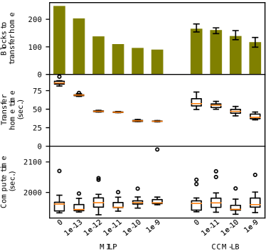
(b) Blocks that need to be sent home, the time required for such transfers, and the compute time for each $\delta$. Gemma was run twelve times on the single Gurobi solution, and once on each of the twelve CCM-LB solutions.

Figure 4: Results comparing the Gurobi (MILP) solutions to CCM-LB.

All experiments were performed on a cluster with 1488 nodes connected with Intel Omni-Path, each composed of 2.9 GHz Intel Cascade Lake 8268 processors with 192 GiB RAM/node. We used two ranks per node (one per socket), with 24 threads each bound to a core on the socket.

VII-A MILP and CCM-LB Comparison

We have implemented the FWMP (cf. §V) for a small-scale Gemma problem using the PuLP [37] library in Python, which outputs a general LP format that can be run with different solvers. From initial testing, we found that the commercial solver, Gurobi [38], far exceeded open-source solvers (such as CBC [39] or GLPK [40]) in speed and quality of solution, and so it was used as the comparison for our distributed load balancer.

This Gemma experimental problem contains 238,738 unknowns across 14 ranks, 1959 tasks, and 206 shared memory blocks with non-zeros. For this set of small-scale experiments, we used the actual task timings from a prior Gemma run, rather than our model described in §VI-D, to reduce the impact of prediction inaccuracies when comparing the two approaches. We note that significant machine noise still results in the task timings deviating from the previous timings.

The Gurobi solver first solves the LP relaxation problem (feasible in polynomial time), whereby the integral constraints are relaxed to real numbers between $[0,1]$. This relaxed, continuous solution is a lower bound on the best possible integral one. Thus, the gap is defined as the relative error between the minimized amount of work ${{\mathcal{W}_{\max}^{i}}}$ and the continuous lower bound ${{\mathcal{W}_{\max}^{l}}}$, i.e., $\nicefrac{{({{\mathcal{W}_{\max}^{i}}}-{{\mathcal{W}_{\max}^{l}}})}}{{{{\mathcal{W}_{\max}^{l}}}}}$.

Figure 4a describes the solutions obtained by the MILP and CCM-LB for varying input values of $\delta$. We configured the solver with a maximum gap of $10^{-4}$, and the MILP columns show the gap that Gurobi found along with the time taken. For the largest value of $\delta$, after more than 46 hours, Gurobi had not found a solution with a gap below $10^{-4}$, suggesting it may not be tractable. We thus decided to terminate this solve, and to time-limit runs to 8 hours for the remaining values of $\delta$. Gurobi ran much faster for smaller values of $\delta$, indicating that the complexity of solving the MILP highly depends on input parameter values. The CCM-LB columns show the ranges of the gaps and the relative increases in ${{\mathcal{W}_{\max}}}$, compared to the best Gurobi solution found. CCM-LB was solved twelve times for each $\delta$, coming up with a different solution each time, and we stopped decreasing $\delta$ once it was clear that the transfer time was near that of $\delta$$=$$0$. The mean time for CCM-LB to find a solution was always under $0.7$ seconds, running online and much faster than the MILP solver.

For all values of $\delta$ except for the largest one, the Gurobi solution gets closer to the optimal (smaller gap), which is expected as CCM-LB is a heuristic-based approach. Interestingly, the heuristic-based CCM-LB in one case finds a better solution that the MILP one ($-0.1\%$) when the FWMP starts to become intractable for Gurobi ($\delta$$=$$10^{-9}$).

Figure 4b depicts the number of blocks $n_{\mathrm{off}}$ that are computed off the home rank, the communication time required to send them home, and the compute time for the same Gemma case, with varying $\delta$ in the CCM model. As $\delta$ increases, $n_{\mathrm{off}}$ should decrease (and the required communication time as well), and this is indeed what we observe: a strong inverse correlation between $\delta$ and $n_{\mathrm{off}}$, demonstrating the validity and efficacy of our model and the relevance of the MILP formulation (FWMP). We also observe that $\delta$ has a larger impact on the number of blocks to be homed, and thus on the homing cost, with the MILP solutions than with CCM-LB; this is because the latter starts from an existing, co-localized configuration, whereas the former computes a solution ab initio. Moreover, we note that compute times across varying $\delta$ and gaps remain within machine noise, despite the fact that gaps are on average slightly worse with CCM-LB.

VII-B Larger-scale Experiments

Ranks	Unknowns	Tasks	Shared blocks
16	243,079	2,383	286
64	488,381	8,955	896
256	983,881	34,709	3,076

(a) Description of the weak-scaled problem. Shared blocks only includes those containing non-zero values.

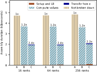
(b) A: baseline Gemma (does not support load balancing); B: overdecomposed Gemma without load balancing; C: overdecomposed Gemma with CCM-LB and $\delta$$=$$10^{-9}$. The above-bar multiplicative factors are the full assembly speedups compared to A for the same number of ranks.

Figure 5: Speedup of the assembly at each scale.

In order to demonstrate our approach at larger scale with a more realistic case, we weak-scaled a similar Gemma problem to three different rank counts, as illustrated in Figure 5a. For these experiments, we created our neural-network model using PyTorch, a popular machine learning framework in Python. We exported trained model weights that can be used in C++ using PyTorch’s libtorch API [41]. The model weights were trained using measurements from a version of Gemma built with an older software stack that exhibited worse computational performance than the configuration used for these benchmarks. As a result, CCM-LB used task time predictions that somewhat differed from the actual, experimental ones; we expect better speedups after retraining the model with the new software stack.

Figure 5b shows the performance we attain, with the “baseline” corresponding to the unchanged Gemma code. By overdecomposing the matrix, we see about a 1.3x speedup due to cache effects from a different kernel size and zero blocks being exposed in the matrix (thus less work being performed). By running our distributed load balancer CCM-LB on the overdecomposed code with tasks, we obtain a 2.3-2.4x speedup up to 256 ranks on the matrix assembly.

VIII Concluding Remarks

Using our proposed reduced-order model (CCM) for describing work in a parallel system with memory constraints, we have demonstrated that our distributed load balancer can find close-to-optimal solutions, leading to substantial speedups in practice for our target application. Because we believe that distributed load balancing research (especially with complex models) should be backed by comparisons to provably-optimal solutions, we have formulated the optimization problem as a mixed-integer linear program. This has allowed us to gauge the optimality of our heuristic-based approach and to demonstrate its veracity. In the future, we plan to show that our model is widely applicable to many parallel algorithms.

Appendix A Proofs of Theorems

See III.1

Proof.

Denoting $\uplus$ the union of two disjoint sets, and because $A$ and $B\setminus{A}$ disjoint with union equal to $A\cup{B}$, we have:

$$\!\!\!{S_{r_{1}}^{p}}\!=\cup_{u\in{T_{r_{1}}^{p}}\!\setminus\!\{t\}}{S_{u}^{p}}\cup{S_{t}^{p}}={{\widetilde{S}}_{r_{1}}^{p}}\!\cup{S_{t}^{p}}={{\widetilde{S}}_{r_{1}}^{p}}\!\uplus({S_{t}^{p}}\!\setminus\!{{\widetilde{S}}_{r_{1}}^{p}}),$$ (33)

$$\!{{\widetilde{S}}_{r_{2}}^{p}}\!=\cup_{u\in{T_{{r_{2}}}^{p}}}{S_{u}^{p}}\cup{S_{t}^{p}}={S_{r_{2}}^{p}}\!\cup{S_{t}^{p}}={S_{r_{2}}^{p}}\!\uplus({S_{t}^{p}}\!\setminus\!{S_{r_{2}}^{p}}).$$ (34)

Thus, by right-distributivity of set difference over set union,

$${S_{r_{1}}^{p}}\!\setminus\!{\widehat{S}_{r_{1}}^{p}}\! =({{\widetilde{S}}_{r_{1}}^{p}}\!\setminus\!{\widehat{S}_{r_{1}}^{p}})\uplus(({S_{t}^{p}}\!\setminus\!{{\widetilde{S}}_{r_{1}}^{p}})\!\setminus\!{\widehat{S}_{r_{1}}^{p}}),$$ (35)

$${{\widetilde{S}}_{r_{2}}^{p}}\!\setminus\!{\widehat{S}_{r_{2}}^{p}}\! =({S_{r_{2}}^{p}}\!\setminus\!{\widehat{S}_{r_{2}}^{p}})\uplus(({S_{t}^{p}}\!\setminus\!{S_{r_{2}}^{p}})\!\setminus\!{\widehat{S}_{r_{2}}^{p}}).$$ (36)

Meanwhile, by definition in (10),

$${{{\widetilde{\mathcal{M}}}_{H}^{p}(r_{1})}} :=\textstyle\sum_{s\in{{\widetilde{S}}_{r_{1}}^{p}}\!\setminus{\widehat{S}_{r_{1}}^{p}}}\!{{\mathcal{M}^{p}\!\left(s\right)}},$$ (37)

$${{{\widetilde{\mathcal{M}}}_{H}^{p}(r_{2})}} :=\textstyle\sum_{s\in{{\widetilde{S}}_{r_{2}}^{p}}\!\setminus{\widehat{S}_{r_{2}}^{p}}}\!{{\mathcal{M}^{p}\!\left(s\right)}},$$ (38)

whence the conclusion, thanks to the disjoint set unions in (35) and (36) that entails additivity of their memory contents. ∎

See V.1

Proof.

By definition of ${S_{r_{i}}^{p}}=\cup_{t_{k}\in{T_{r_{i}}^{p}}}{S_{t_{k}}^{p}}$ (cf. III-A4),

$$\phi_{i,n}=1 \iff s_{n}\in\cup_{t_{k}\in{T_{r_{i}}^{p}}}{S_{t_{k}}^{p}}$$ (39)

$$\iff(\exists k\in{\llbracket 1,{K}\rrbracket})\enskip t_{k}\in{T_{r_{i}}^{p}}\,\land\,s_{n}\in{S_{t_{k}}^{p}}$$ (40)

$$\iff\bigvee_{k=1}^{K}\big{(}\mathds{1}_{T_{r_{i}}^{p}}(t_{k})=1\,\land\,\mathds{1}_{S_{t_{k}}^{p}}(s_{n})=1\big{)}$$ (41)

$$\iff\bigvee_{k=1}^{K}\big{(}\chi^{p}_{i,k}=1\,\land\,u^{p}_{k,n}=1\big{)}$$ (42)

$$\iff\bigvee_{k=1}^{K}\chi^{p}_{i,k}\land u^{p}_{k,n}\,=\,1.$$ (43)

Negating both sides of (43) yields:

$$\phi^{p}_{i,n}=0\iff\bigvee_{k=1}^{K}\chi^{p}_{i,k}\land u^{p}_{k,n}\,=\,0.$$ (44)

Therefore, as $\phi^{p}_{i,n}\!\in{\mathbb{Z}_{2}}$, it follows that

$$(\forall(i{,}n)\in{\llbracket 1,{I}\rrbracket}\!\times\!{\llbracket 1,{N}\rrbracket})\enskip\phi^{p}_{i,n}=\bigvee_{k=1}^{K}\chi^{p}_{i,k}\land u^{p}_{k,n},$$ (45)

whencefrom $(\phi^{p})=(\chi^{p})\odot(u^{p})$ ensues. ∎

See V.2

Proof.

Given any binary values $a$ and $b$, $a\land{}b=ab$, whereas $a\lor{}b=a+b-ab\leq{}a+b$, which, when applied to (45), yields (18). The proof of (17) is done by disjunction elimination: if $\phi_{i,n}=0$, it comes from (44) that both sides in (17) always vanish, making all $K$ inequalities true. If $\phi_{i,n}\!=\!1$, (17) also always holds, irrespective of the value of its right-hand side, which is in ${\mathbb{Z}_{2}}$; all $K$ inequalities are thus true. ∎

See V.3

Proof.

For brevity, we only provide a notional proof, for it is essentially similar to that of Theorem V.1. Applying the same logic, first to the left Boolean product, transforms each slice ${({w}^{p}_{::{m}})}$, a $K\!\times\!K$ task-to-task matrix, into an $I\!\times\!K$ task-to-rank matrix, itself by the right product into an $I\!\times\!I$ rank-to-rank matrix, the ${({\psi}^{p}_{::{m}})}$. ∎

See V.4

Proof.

For all $(i,j)$ and $m$, in ${\llbracket 1,{I}\rrbracket}^{2}$ and ${\llbracket 1,{M}\rrbracket}$, respectively, Theorem V.3 entails that:

$$\psi_{i,j,m}=\bigvee_{\ell=1}^{K}\bigvee_{k=1}^{K}\chi_{i,k}\land w_{k,\ell,m}\land\chi_{j,\ell}$$ (46)

As mentioned above, for a given $m$, $w_{k,\ell,m}$ vanishes for all $k$ and $\ell$, except for a unique couple $(k_{m},\ell_{m})$ corresponding to the task endpoints $t_{k_{m}}$ and $t_{\ell_{m}}$ of the directed communication edge $c_{m}$, for which $w_{k_{m},\ell_{m},m}$$=$$1$. Thus, all but one term in the right-hand side of (46) vanish, and

$$\psi_{i,j,m}=\chi_{i,k_{m}}\land 1\land\chi_{j,\ell_{m}}=\chi_{i,k_{m}}\chi_{j,\ell_{m}}.$$ (47)

The same logic applies to the double sum over $k$ and $\ell$:

$$\sum_{\ell=1}^{K}\sum_{k=1}^{K}\chi_{i,k}\chi_{j,\ell}w_{k,\ell,m}=\chi_{i,k_{m}}\chi_{j,\ell_{m}}=\psi_{i,j,m}.$$ (48)

Although strictly equivalent in integer terms to (24), (48) is not suitable for MILP due the non-linearity in the $\chi$ components in the decision vector $\vec{x}^{p}$ but, by applying the technique first described in [42], we obtain (25) and (26) by alternatively bounding each of these components from above by $1$ and, because $\mathds{1}_{A\cap{}B}$$+$$\mathds{1}_{A\cup{}B}$$=$$\mathds{1}_{A}$$+$$\mathds{1}_{B}$,

$$\chi_{i,k_{m}}\chi_{j,\ell_{m}}\!\!=\chi_{i,k_{m}}\!\!+\chi_{j,\ell_{m}}\!\!-\chi_{i,k_{m}}\!\!\lor\chi_{j,\ell_{m}}\!\geq\chi_{i,k_{m}}\chi_{j,\ell_{m}}\!\!-1\!$$ (49)

which, combined with (48) and the fact that all $w_{i,k,m}$, aside from $w_{k_{m},\ell_{m},m}$$=$$1$, vanish in the double sum, yields (27). ∎

Appendix B Data Reduction Algorithm

Consider a dataset, arranged in a table $\mathcal{T}$ with $n_{r}$ rows of individual observations. Given a target number of rows $n_{r}^{\ast}$, a number of bins $n_{b}$, and a downsampling coefficient $\theta\!\in]0,1[$, our method is described in Algorithm 1.

1:function DynamicDataReduce($n_{r}$, $\mathcal{T}$, $n_{b}$, $\theta$)

2:     $H\leftarrow$Histogram($n_{b}$,$\mathcal{T}$)$\triangleright$ $n_{b}$ bins of rows

3:     $n_{r}^{\scriptscriptstyle-}\leftarrow n_{r}-n_{r}^{\ast}$ $\triangleright$ number of bins to drop

4:     while $n_{r}^{\scriptscriptstyle-}>0$ do

5:         $b_{\max}\leftarrow\operatorname*{arg\,max}_{b\in{}H}$ NumberOfRows($b$)

6:         $n_{\max}\leftarrow$ NumberOfRows($b_{\max}$)

7:         $n\leftarrow\min([\theta\times{}n_{\max}],n_{r}^{\scriptscriptstyle-})$

8:         Randomly remove $n$ rows from $b$.

9:         $n_{r}^{\scriptscriptstyle-}\leftarrow n_{r}^{\scriptscriptstyle-}-n$

10:     end while

11:end function

Algorithm 1 Dynamic data point reduction.

The role of $\theta$ is to arbitrage between convergence speed, and need to obtain a well-balanced distribution in the downsampled histogram: in practice with our dataset, we found a value of $0.5$ to be a good trade-off.

References

- [1] A. Darte, J. M. Mellor-Crummey, R. J. Fowler, and D. G. Chavarría-Miranda, “Generalized multipartitioning of multi-dimensional arrays for parallelizing line-sweep computations,” J. Parallel Distrib. Comput., vol. 63, no. 9, pp. 887–911, 2003.
- [2] C. Reddy and U. Bondhugula, “Effective automatic computation placement and data allocation for parallelization of regular programs,” in Proceedings of the 28th ACM international conference on Supercomputing, 2014, pp. 13–22.
- [3] U. Bondhugula, “Compiling affine loop nests for distributed-memory parallel architectures,” in Proceedings of the International Conference on High Performance Computing, Networking, Storage and Analysis, 2013, pp. 1–12.
- [4] M. Kong, R. Abu Yosef, A. Rountev, and P. Sadayappan, “Automatic generation of distributed-memory mappings for tensor computations,” in Proceedings of the International Conference for High Performance Computing, Networking, Storage and Analysis, 2023, pp. 1–13.
- [5] Ü. V. Çatalyürek and C. Aykanat, “Hypergraph-partitioning-based decomposition for parallel sparse-matrix vector multiplication,” IEEE Trans. Parallel Distrib. Syst., vol. 10, no. 7, pp. 673–693, 1999.
- [6] R. D. Williams, “Performance of dynamic load balancing algorithms for unstructured mesh calculations,” Concurrency: Pract. Exper., vol. 3, pp. 457–481, October 1991.
- [7] R. Das, Y.-S. Hwang, M. Uysal, J. Saltz, and A. Sussman, “Applying the chaos/parti library to irregular problems in computational chemistry and computational aerodynamics,” in Scalable Parallel Libraries Conference, 1993., Proceedings of the, oct 1993, pp. 45 –56.
- [8] B. Hendrickson and R. Leland, “An improved spectral graph partitioning algorithm for mapping parallel computations,” SIAM J. Sci. Comput., vol. 16, pp. 452–469, March 1995.
- [9] Ü. V. Çatalyürek, E. G. Boman, K. D. Devine, D. Bozdag, R. T. Heaphy, and L. A. Riesen, “A repartitioning hypergraph model for dynamic load balancing,” J. Parallel Distrib. Comput., vol. 69, no. 8, pp. 711–724, 2009.
- [10] G. Karypis, K. Schloegel, and V. Kumar, “Parmetis: Parallel graph partitioning and sparse matrix ordering library,” Version 1.0, Dept. of Computer Science, University of Minnesota, 1997.
- [11] K. Devine, B. Hendrickson, E. Boman, M. S. John, and C. Vaughan, “Design of Dynamic Load-Balancing Tools for Parallel Applications,” in Proc. Intl. Conf. Supercomputing, May 2000.
- [12] R. D. Blumofe, C. F. Joerg, B. C. Kuszmaul, C. E. Leiserson, K. H. Randall, and Y. Zhou, “Cilk: an efficient multithreaded runtime system,” in Proceedings of the fifth ACM SIGPLAN symposium on Principles and practice of parallel programming, ser. PPOPP ’95, 1995, pp. 207–216.
- [13] J. Dinan, D. B. Larkins, P. Sadayappan, S. Krishnamoorthy, and J. Nieplocha, “Scalable work stealing,” ser. SC ’09, 2009, pp. 53:1–53:11.
- [14] Y. Yan, J. Zhao, Y. Guo, and V. Sarkar, “Hierarchical place trees: A portable abstraction for task parallelism and data movement,” in Languages and Compilers for Parallel Computing: 22nd International Workshop, LCPC 2009, Newark, DE, USA, October 8-10, 2009, Revised Selected Papers 22. Springer, 2010, pp. 172–187.
- [15] U. A. Acar, G. E. Blelloch, and R. D. Blumofe, “The data locality of work stealing,” ser. SPAA ’00, 2000, pp. 1–12.
- [16] G. Bosilca, A. Bouteiller, A. Danalis, M. Faverge, T. Hérault, and J. J. Dongarra, “Parsec: Exploiting heterogeneity to enhance scalability,” Computing in Science & Engineering, vol. 15, no. 6, pp. 36–45, 2013.
- [17] C. Augonnet, S. Thibault, R. Namyst, and P.-A. Wacrenier, “StarPU: A Unified Platform for Task Scheduling on Heterogeneous Multicore Architectures,” Concurrency and Computation: Practice and Experience, Euro-Par 2009 best papers issue, 2010, accepted for publication, to appear.
- [18] M. Bauer, S. Treichler, E. Slaughter, and A. Aiken, “Legion: Expressing locality and independence with logical regions,” in SC’12: Proceedings of the International Conference on High Performance Computing, Networking, Storage and Analysis. IEEE, 2012, pp. 1–11.
- [19] T. SFX Teixeira, A. Henzinger, R. Yadav, and A. Aiken, “Automated mapping of task-based programs onto distributed and heterogeneous machines,” in Proceedings of the International Conference for High Performance Computing, Networking, Storage and Analysis, 2023, pp. 1–13.
- [20] K. Huang, X. Zhang, D. Zheng, M. Yu, X. Jiang, X. Yan, L. B. de Brisolara, and A. A. Jerraya, “A scalable and adaptable ilp-based approach for task mapping on mpsoc considering load balance and communication optimization,” IEEE Transactions on Computer-Aided Design of Integrated Circuits and Systems, vol. 38, no. 9, pp. 1744–1757, 2019.
- [21] G. Zheng, A. Bhatele, E. Meneses, and L. V. Kale, “Periodic Hierarchical Load Balancing for Large Supercomputers,” International Journal of High Performance Computing Applications (IJHPCA), 2010.
- [22] H. Menon and L. Kalé, “A distributed dynamic load balancer for iterative applications,” in Proceedings of the International Conference on High Performance Computing, Networking, Storage and Analysis, ser. SC ’13. New York, NY, USA: ACM, 2013, pp. 1–11. [Online]. Available: http://doi.acm.org/10.1145/2503210.2503284
- [23] Y. Zhang, G. Chen, G. Sun, and Q. Miao, “Models of parallel computation: a survey and classification,” Frontiers of Computer Science in China, vol. 1, pp. 156–165, 2007.
- [24] A. Aggarwal, A. K. Chandra, and M. Snir, “Communication complexity of prams,” Theoretical Computer Science, vol. 71, no. 1, pp. 3–28, 1990.
- [25] D. Culler, R. Karp, D. Patterson, A. Sahay, K. E. Schauser, E. Santos, R. Subramonian, and T. von Eicken, “Logp: Towards a realistic model of parallel computation,” in Fourth ACM SIGPLAN Symposium on Principles & Practice of Parallel Programming PPOPP, San Diego, CA, May 1993.
- [26] A. Vahdat, D. Becker et al., “Epidemic routing for partially connected ad hoc networks,” 2000.
- [27] A. Demers, D. Greene, C. Hauser, W. Irish, J. Larson, S. Shenker, H. Sturgis, D. Swinehart, and D. Terry, “Epidemic algorithms for replicated database maintenance,” in Proceedings of the sixth annual ACM Symposium on Principles of distributed computing, 1987, pp. 1–12.
- [28] H. M. Wagner, “An integer linear-programming model for machine scheduling,” Naval research logistics quarterly, vol. 6, no. 2, pp. 131–140, 1959.
- [29] “NNSA warhead modernization,” accessed: 2024-03-20. [Online]. Available: https://www.energy.gov/nnsa/articles/warhead-activities-fact-sheet
- [30] R. F. Harrington, “Boundary integral formulations for homogeneous material bodies,” Journal of Electromagnetic Waves and Applications, vol. 3, no. 1, pp. 1–15, 1989.
- [31] S. Rao, D. Wilton, and A. Glisson, “Electromagnetic scattering by surfaces of arbitrary shape,” IEEE Transactions on Antennas and Propagation, vol. 30, no. 3, pp. 409–418, May 1982.
- [32] K. Hornik, M. Stinchcombe, and H. White, “Multilayer feedforward networks are universal approximators,” Neural Networks, vol. 2, no. 5, p. 359–366, 1989. [Online]. Available: http://dx.doi.org/10.1016/0893-6080(89)90020-8
- [33] S. Ioffe and C. Szegedy, “Batch normalization: accelerating deep network training by reducing internal covariate shift,” in International Conference on Machine Learning, vol. 37, 2015, pp. 448–456.
- [34] N. Srivastava, G. Hinton, K. Alex, I. Sutskever, and R. Salakhutdinov, “Dropout: A simple way to prevent neural networks from overfitting,” Journal of Machine Learning Research, vol. 15, pp. 1929–1958, 2014.
- [35] B. Xu, N. Wang, T. Chen, and M. Li, “Empirical evaluation of rectified activations in convolutional network,” arXiv preprint arXiv:1505.00853, 2015.
- [36] I. Loshchilov and F. Hutter, “Decoupled weight decay regularization,” in International Conference on Learning Representations, 2019.
- [37] S. Mitchell, M. OSullivan, and I. Dunning, “Pulp: a linear programming toolkit for python,” The University of Auckland, Auckland, New Zealand, vol. 65, 2011.
- [38] Gurobi Optimization, LLC, “Gurobi Optimizer Reference Manual,” 2023. [Online]. Available: https://www.gurobi.com
- [39] J. Forrest and R. Lougee-Heimer, “Cbc user guide,” in Emerging theory, methods, and applications. INFORMS, 2005, pp. 257–277.
- [40] A. Makhorin, “Glpk (gnu linear programming kit),” http://www. gnu. org/s/glpk/glpk. html, 2008.
- [41] A. Paszke, S. Gross, F. Massa, A. Lerer, J. Bradbury, G. Chanan, T. Killeen, Z. Lin, N. Gimelshein, L. Antiga et al., “Pytorch: An imperative style, high-performance deep learning library,” Advances in neural information processing systems, vol. 32, 2019.
- [42] F. Glover and E. Woolsey, “Converting the 0-1 polynomial programming problem to a 0-1 linear program,” Operations research, vol. 22, no. 1, pp. 180–182, 1974.