Imaginary Stark Skin Effect

Abstract

The non-Hermitian skin effect (NHSE) is a unique phenomenon in non-Hermitian systems. However, studies on NHSE in systems without translational symmetry remain largely unexplored. Here, we unveil a new class of NHSE, dubbed “imaginary Stark skin effect” (ISSE), in a one-dimensional lossy lattice with a spatially increasing loss rate. The energy spectrum of this model exhibits a T-shaped feature, with approximately half of the eigenstates localized at the left boundary. These skin modes exhibit peculiar behaviors, expressed as a single stable exponential decay wave within the bulk region. We use the transfer matrix method to analyze the formation of the ISSE in this model. According to the eigen-decomposition of the transfer matrix, the wave function is divided into two parts, one of which dominates the behavior of the skin modes in the bulk. Our findings provide insights into the NHSE in systems without translational symmetry and contribute to the understanding of non-Hermitian systems in general.

Introduction. —

The study of non-Hermitian quantum physics has gained significant attention in the past two decades due to its unique properties and potential applications in various fields Hatano and Nelson (1996, 1997); Bender and Boettcher (1998); Bender et al. (2002); Rudner and Levitov (2009); Guo et al. (2009); Zeuner et al. (2015); Parto et al. (2018); Bender (2007); Rotter (2009); Regensburger et al. (2012); Zhen et al. (2015); Chen et al. (2017); Hodaei et al. (2017); Feng et al. (2012); St-Jean et al. (2017); El-Ganainy et al. (2018); Xiao et al. (2020); Rüter et al. (2010); Xiao et al. (2017); Poli et al. (2015); Feng et al. (2011); Bahari et al. (2017); Harari et al. (2018); Bandres et al. (2018). One of the intriguing phenomena is the non-Hermitian skin effect (NHSE), namely the boundary localization of an extensive number of eigenstates Martinez Alvarez et al. (2018); Yao and Wang (2018); Yao et al. (2018). The NHSE can lead to novel phenomena absent in its Hermitian counterparts, including unidirectional physical effects Song et al. (2019); Wanjura et al. (2020); Xue et al. (2022), critical phenomena Li et al. (2020); Liu et al. (2020); Yokomizo and Murakami (2021); Guo et al. (2021a), and geometrical related effects in higher dimensions Sun et al. (2021); Zhang et al. (2022a); Li et al. (2022); Zhu and Gong (2022); Wu et al. (2022). The research on the NHSE has motivated a new theoretical framework for non-Hermitian system, known as non-Bloch band theory Yao and Wang (2018); Yokomizo and Murakami (2019); Zhang et al. (2020); Wang et al. (2024), which establishes the concept of the generalized Brillouin zone (GBZ), providing a powerful tool to understand the NHSE and its topological properties Leykam et al. (2017); Shen et al. (2018); Gong et al. (2018); Kawabata et al. (2019a, b); Zhou and Lee (2019); Borgnia et al. (2020); Kawabata et al. (2019c); Xiong (2018); Lee and Thomale (2019); Liu et al. (2019); Lee et al. (2019).

Besides translational symmetric systems, NHSE has also been investigated in systems without translational invariance. However, most of these studies are concentrated on quasicrystals Jiang et al. (2019); Cai (2021); Liu et al. (2021); Yuce and Ramezani (2022); Manna and Roy (2023); Chakrabarty and Datta (2023); Zhou (2023), systems with disorder Longhi (2020); Claes and Hughes (2021); Longhi (2021); Kim and Park (2021); Bhargava et al. (2021); Sarkar et al. (2022); Suthar et al. (2022); Liu et al. (2023) or impurities Li et al. (2021); Roccati (2021); Guo et al. (2021b); Molignini et al. (2023). In this paper, we unveil a new class of NHSE, termed “imaginary Stark skin effect” (ISSE), in a one-dimensional lossy lattice with a nonuniform loss rate. We focus on the case where the loss rate increases with the lattice index and approaches infinity as the lattice index goes to infinity. This scenario resembles a lattice subjected to a leftward imaginary field, which is the meaning of the term ‘imaginary Stark’ in ISSE. We find that the energy spectrum of this model displays a T-shaped feature Yuce and Ramezani (2023), with eigenstates from the upper half of the spectrum localized at the left boundary. Surprisingly, these skin modes exhibit an almost uniform decay rate within the bulk region, despite the broken translational invariance. Moreover, numerical results indicate that these skin modes can be approximately expressed as a single exponential decay wave within the bulk region, which differs from the superposition of two exponential decay waves in conventional NHSE. The broken translational symmetry renders non-Bloch band theory inapplicable for this model. Thus, we analyze these states using the transfer matrix method and reveal the relationship between ISSE and the convergence speed of the transfer matrix eigenvalues. The wave function is divided into two parts based on the eigen-decomposition of the transfer matrix, with one component dominates the behavior of the skin modes in the bulk, thus accounting for the peculiar behavior of ISSE.

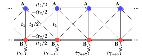
Figure 1: The one-dimensional non-Hermitian lattices with a nonuniform loss rate $\gamma_{n}$.

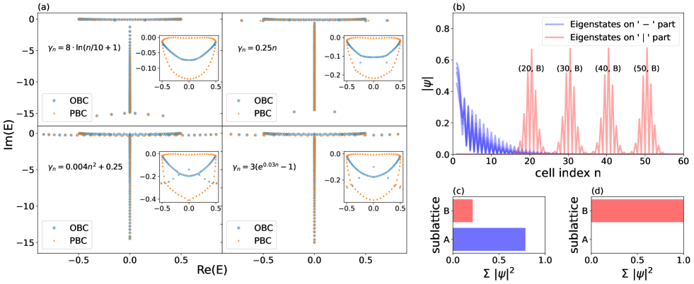
Figure 2: (a) The energy spectrum for logarithmic, linear, quadratic, and exponential loss rate function $\gamma_{n}$. The insets are the ‘$-$’ part of spectra (b) The profile of eigenstates from the ‘$-$’ and ‘$|$’ parts of T-shaped spectrum. The eigenstates are numbered from large imaginary parts to small imaginary parts. 8 eigenstates are displayed, of which 4 are in the ‘$-$’ part (eigenstate 20, 30, 40, 50) and the other 4 are in the‘$|$’ part (eigenstate 80, 90, 100, 110). The coordinate $(n,B)$ is the position of the peak of the eigenstate in the ‘$|$’ part. (c), (d) The average probability of particle in sublattice A and B, $\langle\Sigma_{n}{|\psi_{i}(n,S)|^{2}}\rangle_{\psi_{i}}$, where $S\in\{A,B\}$, and $\psi_{i}$ denotes wave function of eigenstates in ‘$-$’ (c) or ‘$|$’ (d) part of T-shaped spectrum. For (b)-(d), the loss rate $\gamma_{n}=0.25n$. For (a)-(d), $t_{1}=0.4$, $t_{2}=0.5$, and the chain length $L=60$.

Model. —

We consider a one-dimensional lossy lattice [Fig. 1]. The eigenequation of this model is

$$E\psi_{n}^{A}= t_{1}\psi_{n}^{B}+\frac{t_{2}}{2}(\psi_{n-1}^{B}+\psi_{n+1}^{B})+i\frac{t_{2}}{2}(\psi_{n-1}^{A}-\psi_{n+1}^{A}),$$

$$E\psi_{n}^{B}= t_{1}\psi_{n}^{A}+\frac{t_{2}}{2}(\psi_{n-1}^{A}+\psi_{n+1}^{A})-i\frac{t_{2}}{2}(\psi_{n-1}^{B}-\psi_{n+1}^{B})$$

$$-i\gamma_{n}\psi_{n}^{B},$$ (1)

where $\psi_{n}^{A(B)}$ denotes the wave function in sublattices A(B) of unit cell $n$, $L$ is the chain length, and $\gamma_{n}$ represents the loss rate in different B sublattices. When $\gamma_{n}$ is uniform, this model can be transformed to the non-Hermitian Su-Schrieffer-Heeger (SSH) model with asymmetric hopping, whose NHSE has been completely studied Yao and Wang (2018). In this paper, we focus on the case where $\gamma_{n}$ is monotonically increasing with $n$ and satisfies

$$\lim_{n\to\infty}\gamma_{n}\to\infty,$$ (2)

and the situation of open boundary condition (OBC) is mainly considered. The energy spectrum of this model exhibit a T-shaped feature, as shown in Fig. 2(a). Furthermore, the eigenstates in the ‘$-$’ part of T-shaped spectrum exhibit a marked distinction from those in the ‘$|$’ part. The eigenstates in the ‘$-$’ part localize at the left boundary, manifesting the NHSE. This is also supported by the observation that the ‘$-$’ part of periodic boundary condition (PBC) spectra form loops, encircling the ‘$-$’ part of OBC spectra Okuma et al. (2020); Zhang et al. (2020, 2022b), as in Fig. 2(a) inset. Conversely, the eigenstates in the ‘$|$’ part are localized around each sublattice B within the bulk region [Fig. 2(b)]. Notably, the eigenstates in the‘$-$’ part primarily reside in sublattice A [Fig. 2(c)], whereas those in ‘$|$’ part predominantly occupy in sublattice B [Fig. 2(d)]. This observation suggests a relative independence between the chains A and B.

To gain insights, we turn off the coupling between sublattices A and B. Then the model becomes two independent chains A and B. We use $E^{(0)}$ and $E$ to represent energy in A-B decoupled and coupled cases, respectively. The energy of chain A is laid on the real axis with $E^{(0)}=t_{2}\sin k$, whose eigenstates are extended standing waves. In the chain B, each site is linked to an eigenstate localized around it, with an energy closely approximated by its imaginary potential, which is similar to the Wannier-Stark localization Wannier (1962); Hartmann et al. (2004). The superposition of the spectra of chains A and B results in a T-shaped spectrum, where the energy of chain A forms ‘$-$’ part and the energy of chain B forms ‘$|$’ part [Fig. 3(a)]. Upon introducing the coupling between sublattices A and B, the spectrum undergoes certain distortions but retains its overall T-shape [Fig. 3(b)]. For the A-B coupled case, the eigenstates corresponding to the ‘$|$’ part are still localized around their respective sublattices B. However, the NHSE appears in the eigenstates in ‘$-$’ part.

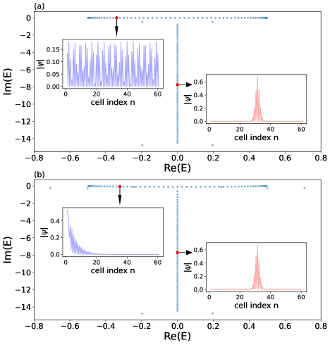
Figure 3: Energy spectrum for turning off (a) and turning on (b) the coupling between sublattices A and B. The left and right insets are profiles of eigenstate 40 and eigenstate 150. The parameters are $t_{1}=0.4$, $t_{2}=0.5$, $\gamma_{n}=0.25n$, and the chain length $L=60$.

ISSE. —

For simplicity, we regard each unit cell as a pseudo spin and perform a $\pi/2$-rotation along the x-axis to each spin. Then the eigenequation becomes a more concise form

$$E\psi_{n}^{A^{\prime}}= -i\frac{\gamma_{n}}{2}\psi_{n}^{A^{\prime}}+t_{2}\psi_{n-1}^{B^{\prime}}+(t_{1}+\frac{\gamma_{n}}{2})\psi_{n}^{B^{\prime}},$$ (3)

$$E\psi_{n}^{B^{\prime}}= -i\frac{\gamma_{n}}{2}\psi_{n}^{B^{\prime}}+(t_{1}-\frac{\gamma_{n}}{2})\psi_{n}^{A^{\prime}}+t_{2}\psi_{n+1}^{A^{\prime}},$$

where $A^{\prime}$ and $B^{\prime}$ are the new Z-basis of pseudo spin after rotation transformation. In the following sections, we will use this basis unless otherwise specified.

The ISSE in this model has two features. First, although the loss rate $\gamma_{n}$ is spatially increasing in the lattice, the skin modes have almost uniform decay rate within the bulk region, illustrated by the wave function’s linearity on a logarithmic scale [Fig. 4(b)]. Second, for one-dimensional spatially periodic tight-binding non-Hermitian models, the eigenstates can be written as a superposition of two exponential decay waves Yokomizo and Murakami (2019),

$$\psi_{n}=(\beta_{m})^{n}\phi^{(m)}+(\beta_{m+1})^{n}\phi^{(m+1)},$$ (4)

To construct continuum bands under open boundary conditions it requires $|\beta_{m}|=|\beta_{m+1}|$, so that two decay waves would generate interference fringes and cancel out each other on the boundary [Fig. 4(a)]. However, in our model, numerical results show the absence of interference fringes, indicating that the skin modes can be approximately expressed as a single exponential decay wave within the bulk region [Fig. 4(b)], i.e.

$$\psi_{n}^{S^{\prime}}\sim(\beta)^{n},$$ (5)

where $S^{\prime}\in\{A^{\prime},B^{\prime}\}$ denotes the sublattice, which is very different from that in spatially periodic models.

We first adopt a rough approach to obtain $\beta$ in Eq. (5). Take the ansatz

$$\psi_{n}^{S^{\prime}}=(\beta+\delta_{n})\psi_{n-1}^{S^{\prime}},$$ (6)

where $\delta_{n}\ll\beta$. Then the bulk eigenequation of Hamiltonian Eq. (3) becomes

$$\left(E+i\frac{\gamma_{n}}{2}\right)\psi_{n}^{A^{\prime}}-\left[t_{1}+\frac{\gamma_{n}}{2}+t_{2}(\beta+\delta_{n})^{-1}\right]\psi_{n}^{B^{\prime}}=0,$$ (7)

$$\left[t_{1}-\frac{\gamma_{n}}{2}+t_{2}(\beta+\delta_{n+1})\right]\psi_{n}^{A^{\prime}}-\left(E+i\frac{\gamma_{n}}{2}\right)\psi_{n}^{B^{\prime}}=0,$$

which leads to

$$0= \gamma_{n}\left\{iE-\frac{t_{2}}{2}\left[(\beta+\delta_{n+1})-(\beta+\delta_{n})^{-1}\right]\right\}$$ (8)

$$+E^{2}-\left[t_{1}+t_{2}(\beta+\delta_{n})^{-1}\right]\left[t_{1}+t_{2}(\beta+\delta_{n+1})\right].$$

To make this equation hold for arbitrary $n$, the $\gamma_{n}$ term $\left\{iE-\frac{t_{2}}{2}\left[(\beta+\delta_{n+1})-(\beta+\delta_{n})^{-1}\right]\right\}$ should be approximate to zero, which has two solutions:

$$\beta_{\pm}\approx\frac{iE}{t_{2}}\left[1\pm\sqrt{1-\left(t_{2}/E\right)^{2}}\right].$$ (9)

The solution $\beta_{-}$ is in agreement with the numerical values of $\beta$.

Transfer matrix method. —

The above approach can not explain why $\beta_{-}$ instead of $\beta_{+}$ fits $\beta$ and how the ISSE arises. In the following part, we analyze the model more accurately via transfer matrix method Kohmoto et al. (1987); Kunst and Dwivedi (2019). Consider the bulk eigen-equation projected on bases $\ket{n-1,B^{\prime}}$ and $\ket{n,A^{\prime}}$: $\bra{n-1,B^{\prime}}H^{\prime}\ket{\psi}=\bra{n-1,B^{\prime}}E\ket{\psi}$ and $\bra{n,A^{\prime}}H^{\prime}\ket{\psi}=\bra{n,A^{\prime}}E\ket{\psi}$, which can be rewritten in terms of transfer matrix as (see details in [SeeSupplementalMaterialat][fordetails.]supp)

$$\ket{\psi(n)}=T(n)\ket{\psi(n-1)},$$ (10)

where $\ket{\psi(n)}=(\psi_{n}^{A^{\prime}},\psi_{n}^{B^{\prime}})^{T}$, and $T(n)$ is the $2\times 2$ transfer matrix between cell $(n-1)$ and cell $n$. The transfer matrix describes the relation of eigenstate wave function between two adjacent cells. If $\gamma_{n}$ is uniform, $T(n)=T=\sum_{i}\lambda_{i}\ket{\lambda_{iR}}\bra{\lambda_{iL}}$ is a constant matrix, and $\ket{\psi(n)}=(T)^{n-1}\ket{\psi(1)}=\sum_{i}\lambda_{i}^{n-1}\braket{\lambda_{iL}}{\psi(1)}\ket{\lambda_{iR}}$, which degenerates to the ansatz of non-Bloch band theory, with $\lambda_{i}$ corresponding to the $\beta_{i}$. In our model, $T(n)$ is a function of $n$, with two eigenvalues, whose eigenequation can be written as:

$$\lambda(n)^{2}+b(n)\lambda(n)+c(n)=0,$$ (11)

where

$$b(n)= \frac{1}{t_{2}\left(t_{1}+\gamma_{n}/2\right)}\Big{[}t_{1}^{2}+t_{2}^{2}-E^{2}+\frac{\gamma_{n}-\gamma_{n-1}}{2}t_{1}$$ (12)

$$-i\frac{\gamma_{n}+\gamma_{n-1}}{2}E\Big{]},$$

$$c(n)= \frac{t_{1}-\gamma_{n-1}/2}{t_{1}+\gamma_{n}/2},$$

we denote these two eigenvalues as $\lambda^{(\pm)}(n)=\frac{1}{2}\left(-b(n)\pm\sqrt{b(n)^{2}-4c(n)}\right)$ with left eigenvectors $\bra{\lambda^{(\pm)}_{L}(n)}$ and right eigenvectors $\ket{\lambda^{(\pm)}_{R}(n)}$, which are orthonormal and complete.

Notice that $b(n)$ and $c(n)$ approach constant value $b_{0}$ and $c_{0}$ as $n$ approaches infinity:

$$\lim_{n\to\infty}b(n)\to b_{0}=-2iE/t_{2},\lim_{n\to\infty}c(n)\to c_{0}=-1,$$ (13)

then we have

$$\lim_{n\to\infty}\lambda^{(\pm)}(n)\to\lambda^{(\pm)}_{0}=\frac{iE}{t_{2}}\left[1\pm\sqrt{1-\left(t_{2}/E\right)^{2}}\right],$$ (14)

which is the same as $\beta_{\pm}$ derived from the rough approach in Eq. (9). Recall that the ‘$-$’ part of T-shaped spectrum is $E_{0}=t_{2}\sin k$ in the A-B decoupled case. Analogously, here we define $\kappa=\arcsin(E/t_{2})$, then Eq. (14) becomes $\lambda_{0}^{(\pm)}=\pm e^{\pm i\kappa}$, which corresponds to the Bloch phase factor $\pm e^{\pm ik}$ in the A-B decoupled case. It’s easy to verify that $|\lambda^{(+)}_{0}|>1$ and $|\lambda^{(-)}_{0}|<1$ [SeeSupplementalMaterialat][fordetails.]supp, which is consistent with the numerical results.

Next, we examine the convergence of $\lambda^{(\pm)}(n)$ towards $\lambda^{(\pm)}_{0}$. As illustrated in Fig. 4(c), $\lambda^{(-)}(n)$ converges notably faster than $\lambda^{(+)}(n)$. Here we give a concise idea of the proof for this observation. For convenience, we assume that $\gamma_{n}$ takes the form of linear function $\gamma_{n}=\gamma_{0}n$. A detailed proof for various types of $\gamma_{n}$ functions can be found in [SeeSupplementalMaterialat][fordetails.]supp. To analyze the speed of convergence, we perform Laurent expansion on $b(n)$, $c(n)$ and $\lambda^{(\pm)}(n)$,

$$b(n) =b_{0}+b_{1}/\gamma_{n}+...,$$ (15)

$$c(n) =c_{0}+c_{1}/\gamma_{n}+...,$$

$$\lambda^{(\pm)}(n) =\lambda^{(\pm)}_{0}+\lambda^{(\pm)}_{1}/\gamma_{n}+....$$

Combine Eq. (11), Eq. (12) and Eq. (15), we can derive

$$\frac{\lambda^{(\pm)}_{1}}{\lambda^{(\pm)}_{0}}=\mp\frac{(t_{1}\pm t_{2}\cos\kappa)(t_{1}\pm t_{2}\cos\kappa+\gamma_{0}/2)}{t_{2}\cos\kappa},$$ (16)

which characterizes the convergence speed of $\lambda^{(\pm)}(n)$ — smaller $\lambda^{(\pm)}_{1}/\lambda^{(\pm)}_{0}$ means smaller $1/\gamma_{n}$ term, and faster convergence. In supplemental material we argue that in the thermodynamic limit the ‘$-$’ part of spectrum in A-B coupled case will be closed to that in decoupled cases [SeeSupplementalMaterialat][forthedetails.]supp, so $\kappa$ can be closely approximated by $k$ in A-B decoupled case, which ranges from $-\pi/2$ to $\pi/2$. Therefore, from Eq. (16), it follows that $|\lambda^{(-)}_{1}/\lambda^{(-)}_{0}|<|\lambda^{(+)}_{1}/\lambda^{(+)}_{0}|$. In particular, $|\lambda^{(-)}_{1}/\lambda^{(-)}_{0}|$ approaches zero when $\cos\kappa$ is near $t_{1}/t_{2}$ or $(t_{1}+\gamma_{0}/2)/t_{2}$, which leads to a much faster convergence speed of $\lambda^{(-)}(n)$.

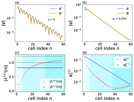
Figure 4: (a), (b) The profile of eigenstates for uniform loss rate and linear loss rate. For uniform loss rate, two exponential decay waves generate interference fringe in the bulk, while for linear loss rate case, only one exponential decay wave dominates the wave function. (c) The modulus of eigenvalues of transfer matrix $|\lambda^{(\pm)}(n)|$ as a function of $n$. The three horizontal black lines from top to bottom are $\lambda^{(+)}_{0}$, $1$, $\lambda^{(-)}_{0}$. (d) The decomposition component of wave function, $\psi^{(\pm)}_{n}$, varies with $n$. The parameters are $t_{1}=0.4$, $t_{2}=0.5$, chain length $L=60$, $\gamma=5$ for (a) and $\gamma_{n}=0.25n$ for (b)-(d).

Now we can analyze the formation of the ISSE states in this model. We decompose $\ket{\psi(n)}$ to the eigenvectors of $T(n)$,

$$\ket{\psi(n)}=\psi_{n}^{(+)}\ket{\lambda^{(+)}_{R}(n)}+\psi_{n}^{(-)}\ket{\lambda^{(-)}_{R}(n)},$$ (17)

where $\psi_{n}^{(\pm)}=\braket{\lambda^{(\pm)}_{L}(n)}{\psi(n)}$, denoting the $\bra{\lambda^{(\pm)}_{L}(n)}$ component of $\ket{\psi(n)}$. If $\gamma_{n}$ is uniform, along with Eq. (10), we get the relation between $\psi_{n-1}^{(\pm)}$ and $\psi_{n}^{(\pm)}$: $\psi_{n}^{(\pm)}=\lambda^{(\pm)}\psi_{n-1}^{(\pm)}$. This is straightforward—the $\bra{\lambda^{(\pm)}_{L}}$ component, $\psi_{n}^{(\pm)}$, is scaled by the corresponding eigenvalue $\lambda^{(\pm)}$. Back to the nonuniform $\gamma_{n}$, we can take the approximation that [SeeSupplementalMaterialat][forthedetails.]supp

$$\psi_{n}^{(\pm)}\approx\lambda^{(\pm)}(n)\psi_{n-1}^{(\pm)}.$$ (18)

Fig. 4(d) shows how $\psi_{n}^{(\pm)}$ evolves with $n$. The component of $\ket{\psi(n)}$, $\psi_{n}^{(+)}$ and $\psi_{n}^{(-)}$, should be in the same order at two edges, so they can cancel out each other to satisfy OBCs $\ket{\psi(0)}=\ket{\psi(L+1)}=0$. Then we divide the wave function into three stages for different $n$, as shown in Fig. 4(c) and Fig. 4(d). These three stages can be roughly viewed as the left boundary region, the bulk region, and the right boundary region. In the first stage, near the left boundary, $\psi_{n}^{(+)}$ and $\psi_{n}^{(-)}$ begin at the same order. $\lambda^{(-)}(n)$ converges to $\lambda^{(-)}_{0}$ quickly, so according to Eq. (18), $\psi_{n}^{(-)}$ acts as an exponential decay wave $\psi_{n}^{(-)}\sim\left(\lambda^{(-)}_{0}\right)^{n}$. While when $\gamma_{n}$ increases from 0 and approaches $2t_{1}$, $\lambda^{(+)}(n)=c(n)/\lambda^{(-)}(n)\approx(t_{1}-\gamma_{n-1}/2)/\left[(t_{1}+\gamma_{n}/2)\lambda^{(-)}_{0}\right]$ would be near $0$, hence $|\psi_{n}^{(+)}|$ would diminish at a significantly faster rate than $|\psi_{n}^{(-)}|$, eventually attenuating to an extremely low value. In the second stage, in the middle of eigenstate wave function, $|\psi_{n}^{(+)}|$ is lower several orders than $|\psi_{n}^{(-)}|$, so $\psi_{n}^{(-)}$ will dominate the behavior of $\ket{\psi(n)}$ and keep the rigorously exponentially decaying. As $n$ increases, $|\lambda^{(+)}(n)|$ keeps increasing to approach $|\lambda^{(+)}_{0}|$, and after $|\lambda^{(+)}(n)|$ exceeding $1$, we enter the last stage, near the right boundary. In this stage, since $|\lambda^{(+)}(n)|>1$, $|\psi_{n}^{(+)}|$ reverses the decline, starts to increase, and finally approaches the order of $|\psi_{n}^{(-)}|$ at the right boundary to meet the OBC. Review these three stages, we see that $|\psi_{n}^{(-)}|$ is much larger than $|\psi_{n}^{(+)}|$ in the bulk, so the $\psi_{n}^{(-)}\ket{\lambda^{(-)}_{R}(n)}$ part dominates the behavior of $\ket{\psi(n)}$, which scales as $\left(\lambda^{(-)}_{0}\right)^{n}$. The influence of $\psi_{n}^{(+)}\ket{\lambda^{(+)}_{R}(n)}$ part becomes apparent only near the boundary, causing fluctuations in wave function at these areas [Fig. 4(b)].

Our analysis shows that the formation of the ISSE in this model demands notably fast convergence speed of $\lambda^{(-)}(n)$, which leads to a single stable exponential decay wave predominantly governs the behavior of the skin modes in the bulk. We discuss the impact of parameters in [SeeSupplementalMaterialat][forthedetails.]supp. An extremely small or large $t_{1}$ compared with $t_{2}$ would result in a sluggish convergence speed of $\lambda^{(-)}(n)$, which would weaken the features of ISSE. This also supports the relationship between the ISSE and the convergence speed of $\lambda^{(-)}(n)$. Furthermore, we demonstrate that it’s possible to exhibit the ISSE in a short lattice, which provides the feasibility of future experimental investigation with finite-size systems on this model [SeeSupplementalMaterialat][forthedetails.]supp.

Conclusions. —

We investigate a non-Hermitian lattice with nonuniform loss rate. In this model, only almost half of eigenstates exhibit the NHSE with intriguing features, which differ from conventional NHSE. Using the transfer matrix method, we show that the convergence speed of the transfer matrix eigenvalues plays a crucial role in the formation of ISSE. We divide the wave function into two parts according to the eigen-decomposition of the transfer matrix. One part is an exponential decay wave that dominates the behavior of the wave function. While the other part is extremely small within the bulk, and only has a significant effect on the boundary. Our work provides a new perspective on the non-Hermitian systems without translational symmetry.