REBEL: Reinforcement Learning via Regressing
Relative Rewards

Abstract

While originally developed for continuous control problems, Proximal Policy Optimization (PPO) has emerged as the work-horse of a variety of reinforcement learning (RL) applications including the fine-tuning of generative models. Unfortunately, PPO requires multiple heuristics to enable stable convergence (e.g. value networks, clipping) and is notorious for its sensitivity to the precise implementation of these components. In response, we take a step back and ask what a minimalist RL algorithm for the era of generative models would look like. We propose REBEL, an algorithm that cleanly reduces the problem of policy optimization to regressing the relative rewards via a direct policy parameterization between two completions to a prompt, enabling strikingly lightweight implementation. In theory, we prove that fundamental RL algorithms like Natural Policy Gradient can be seen as variants of REBEL, which allows us to match the strongest known theoretical guarantees in terms of convergence and sample complexity in the RL literature. REBEL can also cleanly incorporate offline data and handle the intransitive preferences we frequently see in practice. Empirically, we find that REBEL provides a unified approach to language modeling and image generation with stronger or similar performance as PPO and DPO, all while being simpler to implement and more computationally tractable than PPO.

1 Introduction

The generality of the reinforcement learning (RL) paradigm is striking: from continuous control problems (Kalashnikov et al., 2018) to, recently, the fine-tuning of generative models (Stiennon et al., 2022; Ouyang et al., 2022), RL has enabled concrete progress across a variety of decision-making tasks. Specifically, when it comes to fine-tuning generative models, Proximal Policy Optimization (PPO, Schulman et al. (2017)) has emerged as the de-facto RL algorithm of choice, from language models (LLMs) (Ziegler et al., 2020; Stiennon et al., 2022; Ouyang et al., 2022; Touvron et al., 2023) to image generative models (Black et al., 2023; Fan et al., 2024; Oertell et al., 2024).

If we take a step back however, it is odd that we are using an algorithm designed for optimizing two-layer networks for continuous control tasks from scratch for fine-tuning the billions of parameters of modern-day generative models. In the continuous control setting, the randomly initialized neural networks and the possible stochasticity in the dynamics necessitate variance reduction through a learned value function as a baseline (Schulman et al., 2015b), while clipping updates is important to limit distribution shift from iteration to iteration (Kakade and Langford, 2002). This means that when applied to generative model fine-tuning, we need to store four models in memory simultaneously (the policy, the reference policy, the critic, and the reward model), each with billions of parameters. Furthermore, we often add a KL regularization to the base model for fine-tuning, making explicit clipping unnecessary nor advisable, as pointed out by Ahmadian et al. (2024). Even outside of the generative modeling context, PPO is notorious for the wide range of performances measured, with differences being attributed to seemingly inconsequential implementation details (Henderson et al., 2019; Engstrom et al., 2020). This begs the question:

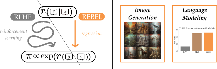
Figure 1: We present REBEL: a simple and scalable RL algorithm that performs policy optimization via iteratively regressing the difference in rewards directly in terms of the policy. This allows us to eliminate much of the complexity (e.g. value functions, clipping) of algorithms like PPO (Schulman et al., 2017). We apply REBEL to problems in both image generation and language modeling and find that despite its conceptual and implementation-level simplicity, REBEL is able to match or sometimes outperform the performance of PPO while out-performing purely offline techniques like DPO (Rafailov et al., 2023).

Are there simpler algorithms that scale to modern RL applications?

Our answer is REBEL: an algorithm that reduces the problem of reinforcement learning to solving a sequence of squared loss regression problems on iteratively collected datasets. The regression problems directly use policies to predict the difference in rewards. This allows us to eliminate the complexity of value functions, avoid heuristics like clipping, and scale easily to problems in both language modeling and image generation. Our key insight is that regressing relative rewards via policies directly on a sequence of iteratively collected datasets implicitly enables policy improvement.

Rather than being a heuristic, REBEL comes with strong guarantees in theory and can be seen as a strict generalization of classical techniques (e.g., NPG) in reinforcement learning. Furthermore, REBEL cleanly incorporates offline datasets when available, can be extended to robustly handle intransitive preferences (Swamy et al., 2024), and empirically out-performs techniques like PPO and DPO (Rafailov et al., 2023) in language generation and has a faster convergence with a similar asymptotic performance in image generation. More explicitly, our key contributions are four-fold:

1. We propose REBEL, a simple and scalable RL algorithm. REBEL finds a near-optimal policy by solving a sequence of least square regression problems on iteratively collected datasets. Each regression problem involves using a policy-parameterized regressor to predict the difference in rewards across trajectories sampled from the dataset. This dataset can be generated in a purely on-policy fashion or can incorporate offline data, enabling hybrid training. Furthermore, REBEL can be easily extended to handle intransitive preferences.

2. We connect REBEL to classical RL methods. We show that REBEL is a generalization of the foundational Natural Policy Gradient (NPG, Kakade (2001)) algorithm – applying the Gauss-Newton algorithm to the sequence of regression problems that REBEL solves recovers NPG. However, by instead applying simpler first-order optimization techniques, we are able to avoid computing the Fisher Information Matrix and enjoy a variance reduction effect. Thus, REBEL can be understood as a generalization of NPG while being much more scalable.

3. We analyze the convergence properties of REBEL. We prove via a direct reduction-based analysis that as long as we can solve the regression problem well at each iteration, we will be able to compete with any policy covered by the iteratively collected datasets (matching the strongest known results in the agnostic RL). These problems involve predicting the difference in rewards between trajectories in our dataset. We expect this problem to be well-solved in practice because our class of regressors is isomorphic to a class of policies that is highly expressive for the applications we consider (i.e. flexible Transformer models).

4. We evaluate REBEL both on language modeling and image generation tasks. We find that the on-policy version of REBEL outperforms PPO and DPO on language modeling and has similar performance for image generation tasks. On the TL;DR summarization task, we show REBEL scales well by finetuning a 6.9B parameter model. For text-guided image generation, REBEL optimizes a consistency model that converges to a similar performance as PPO.

In short, REBEL is a simple and scalable algorithm that enjoys strong theoretical guarantees and empirical performance. We believe it is a suitable answer to the question raised above.

2 REBEL: REgression to RElative REward Based RL

We first outline the notation used throughout the paper.

2.1 Notation

We consider the Contextual Bandit formulation (Langford and Zhang, 2007) of RL which has been used to formalize the generation process of models like LLMs (Rafailov et al., 2023; Ramamurthy et al., 2022; Chang et al., 2023) and Diffusion Models (Black et al., 2023; Fan et al., 2024; Oertell et al., 2024) due to the determinism of the transitions. More explicitly, in the deterministic transition setting, explicit states are not required as they can be equivalently represented by a sequence of actions. Furthermore, the entire sequence of actions can be considered as a single “arm” in a bandit problem with an exponentially large action space.

We denote by $(x,y)$ a prompt/response pair with $x\in\mathcal{X}$ as a prompt and $y\in\mathcal{Y}$ as a response (e.g., a sequence of tokens, or in general a sequence of actions). We assume access to a reward function $r(x,y)$ from which we can query for reward signals (the exact form of $r$ does not need to be known). Querying $r$ at $(x,y)$ will return a scalar $r(x,y)$ measuring the quality of the response. Such a reward function could be a pre-defined metric (e.g., Rouge score against human responses) or it could be learned from an offline human demonstration or preference data (e.g., the RLHF paradigm (Christiano et al., 2017; Ziegler et al., 2020)), as explored in our experiments.

Denote by $\pi\in\mathcal{X}\mapsto\Delta(Y)$, a policy (e.g. LLM) that maps from a prompt $x$ to a distribution over the response space $\mathcal{Y}$. We use $\rho$ to denote the distribution over prompts (i.e. initial states / contexts) $x$. Throughout the paper, we use $\pi_{\theta}(y|x)$ to denote a parameterized policy with parameter $\theta$ (e.g., a neural network policy). At times we interchangeably use $\pi_{t}$ and $\pi_{\theta_{t}}$ when it is clear from the context. We emphasize that while we focus on the bandit formulation for notation simplicity, the algorithms proposed here can be applied to any deterministic MDP where $x$ is the initial state and the trajectory $y$ consists of the sequence of actions.

At each iteration of all algorithms, our goal will be to solve the following KL-constrained RL problem:

$$\pi_{t+1}=\mathop{\mathrm{argmax}}_{\pi}\mathbb{E}_{x,y\sim\pi(\cdot|x)}r(x,y)-\frac{1}{\eta}\mathbb{E}_{x}\text{KL}\left(\pi(\cdot|x)||\pi_{t}(\cdot|x)\right).$$ (1)

Intuitively, this can be thought of asking for the optimizer to fine-tune the policy $\pi_{t+1}$ according to $r$ while staying close to some baseline policy $\pi_{t}$.

2.2 Deriving REBEL: REgression to RElative REward Based RL

From Ziebart et al. (2008), we know that there exists a closed-form solution to the above minimum relative entropy problem (Eq. 1, Grünwald and Dawid (2004)):

$$\forall x,y:\pi_{t+1}(y|x)=\frac{\pi_{t}(y|x)\exp(\eta r(x,y))}{Z(x)};\;Z(x)=\sum_{y}\pi_{t}(y|x)\exp(\eta r(x,y)).$$ (2)

As first pointed out by Rafailov et al. (2023), observe that we can invert Eq. 2 and write the reward as a function of the policy, i.e. the “DPO Trick”:

$$\forall x,y:r(x,y)=\frac{1}{\eta}\left(\ln(Z(x))+\ln\left(\frac{\pi_{t+1}(y|x)}{\pi_{t}(y|x)}\right)\right).$$ (3)

As soon as $\mathcal{X}$ and $\mathcal{Y}$ become large, we can no longer guarantee the above expression holds exactly at all $(x,y)$ and therefore need to turn our attention to choosing a policy such that Eq. 3 is approximately true. We propose using a simple square loss objective between the two sides of Eq. 3 to measure the goodness of a policy, i.e. reducing RL to a regression problem:

$$\left(r(x,y)-\frac{1}{\eta}\left(\ln(Z(x))+\ln\left(\frac{\pi_{t+1}(y|x)}{\pi_{t}(y|x)}\right)\right)\right)^{2}.$$ (4)

Unfortunately, this loss function includes the partition function $Z(x)$, which can be challenging to approximate over large input / output domains. However, observe that $Z(x)$ only depends on $x$ and not $y$. Thus, if we have access to paired samples, i.e. $(x,y)$ and $(x,y^{\prime})$, we can instead regress the difference in rewards to eliminate this term from our objective:

$$\left((r(x,y)-r(x,y^{\prime}))-\frac{1}{\eta}\left(\ln\left(\frac{\pi_{t+1}(y|x)}{\pi_{t}(y|x)}\right)-\ln\left(\frac{\pi_{t+1}(y^{\prime}|x)}{\pi_{t}(y^{\prime}|x)}\right)\right)\right)^{2}.$$ (5)

Of course, we need to evaluate this loss function on some distribution of samples. In particular, we propose using an on-policy dataset $\mathcal{D}_{t}=\{x,y,y^{\prime}\}$ with $x\sim\rho,y\sim\pi_{t}(\cdot|x),y^{\prime}\sim\mu(\cdot|x)$, where $\mu$ is some base distribution. The base distribution $\mu$ can either be a fixed offline dataset (e.g. the instruction fine-tuning dataset) or $\pi_{t}$ itself. Thus, the choice of base distribution $\mu$ determines whether REBEL is hybrid or fully online. Putting it all together, we arrive at our core REBEL objective:

$$\sum_{(x,y,y^{\prime})\in\mathcal{D}_{t}}\left((r(x,y)-r(x,y^{\prime}))-\frac{1}{\eta}\left(\ln\left(\frac{\pi_{t+1}(y|x)}{\pi_{t}(y|x)}\right)-\ln\left(\frac{\pi_{t+1}(y^{\prime}|x)}{\pi_{t}(y^{\prime}|x)}\right)\right)\right)^{2}.$$ (6)

To recap, given a pair of completions $y,y^{\prime}$ to a prompt $x$, REBEL attempt to fit the relative reward

$$r(x,y)-r(x,y^{\prime})$$ (7)

by optimizing over a class of predictors of the form

$$\frac{1}{\eta}\left(\ln\frac{\pi_{\theta}(y|x)}{\pi_{\theta_{t}}(y|x)}-\ln\frac{\pi_{\theta}(y^{\prime}|x)}{\pi_{\theta_{t}}(y^{\prime}|x)}\right).$$ (8)

Critically, observe that if we were able to perfectly solve this regression problem, we would indeed recover the optimal solution to the KL-constrained RL problem we outlined in Eq. 1. While the above update might seem somewhat arbitrary at first glance, it has deep connections to prior work in the literature that illuminate its strengths over past techniques. We now discuss some of them.

Algorithm 1 REgression to RElative REward Based RL (REBEL)

1:  Input: Reward $r$, policy class $\Pi=\{\pi_{\theta}\}$, base distribution $\mu$, learning rate $\eta$

2:  Initialize policy $\pi_{\theta_{0}}$.

3:  for $t=0$ to $T-1$ do

4:     // Base distribution $\mu$ can either be an offline dataset or $\pi_{t}$.

5:     Collect dataset $\mathcal{D}_{t}=\{x,y,y^{\prime}\}$ where $x\sim\rho,y\sim\pi_{t}(\cdot|x),y^{\prime}\sim\mu(\cdot|x)$

6:     Solve square loss regression problem:

$$\theta_{t+1}=\mathop{\mathrm{argmin}}_{\theta}\sum_{(x,y,y^{\prime})\in\mathcal{D}_{t}}\left(\frac{1}{\eta}\left(\ln\frac{\pi_{\theta}(y|x)}{\pi_{\theta_{t}}(y|x)}-\ln\frac{\pi_{\theta}(y^{\prime}|x)}{\pi_{\theta_{t}}(y^{\prime}|x)}\right)-\left(r(x,y)-r(x,y^{\prime})\right)\right)^{2}$$ (9)

7:  end for

3 Understanding REBEL as an Adaptive Policy Gradient

We begin by recapping the foundational algorithms for policy optimization before situating REBEL within this space of techniques.

3.1 Adaptive Gradient Algorithms for Policy Optimization

In this section, we give a brief overview of three adaptive gradient algorithms: Mirror Descent (MD), Natural Policy Gradient (NPG), and Proximal Policy Optimization (PPO). We discuss why they are preferable to their non-adaptive counterparts (Gradient Descent (GD) and Policy Gradient (PG)) and the connections between them.

Mirror Descent. If $\mathcal{X}$ and $\mathcal{Y}$ are small discrete spaces (i.e. we are in the tabular setting), we can used the closed-form expression for the minimum relative entropy problem (Eq. 2). This is equivalent to the classic Mirror Descent (MD) algorithm with KL as the Bregman divergence. This update procedure is also sometimes known as soft policy iteration (Ziebart et al., 2008). Note that it does not even involve a parameterized policy and is therefore manifestly covariant. MD ensures a $1/T$ convergence rate, i.e., after $T$ iterations, it must find a policy $\hat{\pi}$, such that $\mathbb{E}_{x,y\sim\pi^{\star}(.|x)}r(x,y)-\mathbb{E}_{x,y\sim\hat{\pi}(.|x)}r(x,y)\leq O(1/T)$. In particular, the convergence is almost dimension-free: the convergence rate scales logarithmically with respect to the size of the $\mathcal{Y}$ space. Note that gradient ascent will not enjoy such a dimension-free rate when optimizing over the simplex. When $\sup_{x,y}|r(x,y)|$ is bounded, we can show that the KL divergence between two policies, i.e., $\text{KL}(\pi_{t+1}(\cdot|x)||\pi_{t}(\cdot|x))$, is also bounded, ensuring $\pi_{t+1}$ stay close to $\pi_{t}$. One can also show monotonic policy improvement, i.e., $\mathbb{E}_{x,y\sim\pi_{t+1}}r(x,y)\geq\mathbb{E}_{x,y\sim\pi_{t}}r(x,y)$. Foreshadowing a key point we will soon expound upon, both NPG and PPO can be considered approximations of this idealized tabular policy update procedure.

Natural Policy Gradient. When $\mathcal{Y}$ and $\mathcal{X}$ are large, we cannot simply enumerate all $x$ and $y$. Thus, we need to use a function to approximate $\pi$, which makes it impossible to exactly implement Eq. 2. Let us use $\pi_{\theta}$ to denote a parameterized policy with parameter $\theta$ (e.g. the weights of a transformer). The Natural Policy Gradient (NPG, Kakade (2001)) approximates the KL in Equation 1 via its second-order Taylor expansion, whose Hessian is known as the Fisher Information Matrix (FIM, Bagnell and Schneider (2003)), i.e.

$$\mathbb{E}_{x}\text{KL}(\pi_{\theta}(\cdot|x)||\pi_{\theta_{t}}(\cdot|x))\approx(\theta-\theta_{t})^{\top}\underbrace{\mathbb{E}_{x,y\sim\pi_{\theta_{t}}(\cdot|x)}\left[\nabla\ln\pi_{\theta_{t}}(y|x)\nabla\ln\pi_{\theta_{t}}(y|x)^{\top}\right]}_{\text{Fisher Information Matrix }F_{t}}(\theta-\theta_{t}).$$

The NPG update can be derived by plugging in this approximation to Eq. 1, further approximating the $\mathbb{E}_{x,y\sim\pi_{\theta}(\cdot|x)}r(x,y)$ by its first order Taylor expansion around $\theta_{t}$, and finding the root of the resulting quadratic form:

$$\theta_{t+1}=\theta_{t}+\eta F_{t}^{\dagger}\left(\mathbb{E}_{x,y\sim\pi_{\theta_{t}}(\cdot|x)}\nabla\ln\pi_{\theta_{t}}(y|x)r(x,y)\right)$$ (10)

where $F_{t}^{\dagger}$ is pseudo-inverse of $F_{t}$, and $\mathbb{E}_{x,y\sim\pi_{\theta_{t}}(\cdot|x)}\nabla\ln\pi_{\theta_{t}}(y|x)r(x,y)$ is the standard policy gradient (i.e. REINFORCE (Williams, 1992)). As mentioned above, this update procedure can be understood as performing gradient updates in the local geometry induced by the Fisher information matrix, which ensures that we are taking small steps in policy space rather than in parameter space. Conversely, unlike regular gradient descent methods (i.e., PG), NPG allows us to make large changes in the parameter space $\Theta$, as long as the resulting two policies are close to each other in terms of KL divergence. This property allows NPG to make more aggressive and adaptive updates in the parameter space of the policy as well as be invariant to linear transformations of the parameters. Theoretically, Agarwal et al. (2021a) show that NPG with softmax parameterization converges at the $1/T$ rate in a dimension-free manner, provably faster than the standard PG under the same setup. Empirically, the superior convergence speed of NPG compared to that of PG was observed in its original exploration (Kakade, 2001; Bagnell and Schneider, 2003), as well as in follow-up work like TRPO (Schulman et al., 2015a). Critically, while elegant in theory, NPG, unfortunately, does not scale to modern generative models due to the need for computing the Fisher matrix inverse either explicitly or implicitly via the Hessian-vector matrix product trick.

Proximal Policy Optimization. To address the scalability of NPG, Schulman et al. (2017) proposes Proximal Policy Optimization (PPO). Rather than explicitly computing the KL divergence between policies or approximating it via a Taylor expansion, PPO takes a more direct route and uses clipped updates with the hope of controlling the action probability deviation from $\pi_{\theta_{t+1}}$ to $\pi_{\theta_{t}}$, i.e.

$$\theta_{t+1}:=\mathop{\mathrm{argmax}}_{\theta}\mathbb{E}_{x,y\sim\pi_{\theta_{t}}(\cdot|x)}\text{clip}\left(\frac{\pi_{\theta}(y|x)}{\pi_{\theta_{t}}(y|x)};1-\epsilon,1+\epsilon\right)r(x,y).$$ (11)

Prima facie, this update follows the underlying intuition of NPG: allow big and adaptive changes in the policy’s parameters $\theta$, as long as the corresponding action probabilities do not change too much. This perhaps explains the superiority of PPO over vanilla REINFORCE in domains like continuous control. Unfortunately, under closer scrutiny, it becomes apparent that PPO-style clipped updates neither guarantee closeness to the prior policy nor have NPG-style adaptivity. While the clipping operator can set the gradient to be zero at samples $(x,y)$ where $\pi_{\theta_{t+1}}(y|x)$ is much larger or smaller than $\pi_{\theta_{t}}(y|x)$, it cannot actually guarantee $\pi_{\theta_{t+1}}$ staying close to $\pi_{\theta_{t}}$, a phenomenon empirically observed in prior work (Hsu et al., 2020). Furthermore, hard clipping is not adaptive – it treats all $(x,y)$ equally and clips whenever the ratio is outside of a fixed range. In contrast, constraining the KL divergence to the prior policy allows one to vary the ratio $\pi(y|x)/\pi_{t}(y|x)$ at different $(x,y)$, as long as the total KL divergence across the state space is small. Lastly, clipping reduces the effective size of a batch of training examples and thus wastes training samples.

A REBEL With a Cause. Our algorithm REBEL addresses the limitations of NPG (scalability) and PPO (lack of conservativity or adaptivity) from above. First, unlike NPG, it does not rely on the Fisher information matrix at all and can easily scale to modern LLM applications, yet (as we will discuss below) can be interpreted as a generalization of NPG. Second, in contrast to PPO, it doesn’t have unjustified heuristics and thus enjoys strong convergence and regret guarantees just like NPG.

3.2 Connections between REBEL and MD / NPG

We now sketch a series of connections between REBEL and the methods outlined above.

Exact REBEL is Mirror Descent. First, to build intuition, we interpret our algorithm’s behavior under the assumption that the least square regression optimization returns the exact Bayes Optimal solution (i.e., our learned predictor achieves zero prediction error everywhere):

$$\forall x,y,y^{\prime}:\quad\frac{1}{\eta}\left(\ln\frac{\pi_{\theta_{t+1}}(y|x)}{\pi_{\theta_{t}}(y|x)}-\ln\frac{\pi_{\theta_{t+1}}(y^{\prime}|x)}{\pi_{\theta_{t}}(y^{\prime}|x)}\right)=r(x,y)-r(x,y^{\prime})$$ (12)

Conditioned on Eq. 12 being true, a few lines of algebraic manipulation reveals that there must exist a function $c(x)$ which is independent of $y$, such that:

$$\forall x,y:\quad\frac{1}{\eta}\ln\frac{\pi_{\theta_{t+1}}(y|x)}{\pi_{\theta_{t}}(y|x)}=r(x,y)+c(x).$$

Taking an $\exp$ on both sides and re-arrange terms, we get:

$$\forall x,y:\quad\pi_{\theta_{t+1}}(y|x)\propto\pi_{\theta_{t}}(y|x)\exp\left(\eta r(x,y)\right).$$

In other words, under the strong assumption that least square regression returns a point-wise accurate estimator (i.e., Eq. 12), we see the REBEL recovers the exact MD update, which gives it (a) a fast $1/T$ convergence rate (Shani et al., 2020; Agarwal et al., 2021a), (b) conservativity, i.e., $\max_{x}\text{KL}(\pi_{t+1}(\cdot|x)||\pi_{t}(\cdot|x))$ is bounded as long as $\max_{x,y}|r(x,y)|$ is bounded, and (c) monotonic policy improvement via the NPG standard analysis (Agarwal et al., 2021a).

NPG is Approximate REBEL with Gauss-Newton Updates. We provide another interpretation of REBEL by showing that NPG (Eq. 10) can be understood as a special case of REBEL where the least square problem in Eq. 9 is approximately solved via a single iteration of the Gauss-Newton algorithm.

As for any application of Gauss-Newton, we start by approximating our predictor $\frac{1}{\eta}\ln\pi_{\theta}(y|x)/\pi_{\theta_{t}}(y|x)$ by its first order Taylor expansion at $\theta_{t}$:

$$\frac{1}{\eta}\left(\ln\pi_{\theta}(y|x)-\ln\pi_{\theta_{t}}(y|x)\right)\approx\frac{1}{\eta}\nabla_{\theta}\ln\pi_{\theta_{t}}(y|x)^{\top}(\theta-\theta_{t}),$$

where $\approx$ indicates that we ignore higher order terms in the expansion. If we $\delta:=\theta-\theta_{t}$ and replace $\frac{1}{\eta}\left(\ln\pi_{\theta}(y|x)-\ln\pi_{\theta_{t}}(y|x)\right)$ by its above first order approximation in Eq. 9, we arrive at the following quadratic form:

$$\min_{\delta}\mathbb{E}_{x\sim\rho,y\sim\pi_{\theta_{t}}(\cdot|x),y^{\prime}\sim\mu(\cdot|x)}\left(\frac{1}{\eta}\left(\nabla_{\theta}\ln\pi_{\theta_{t}}(y|x)-\nabla_{\theta}\ln\pi_{\theta_{t}}(y^{\prime}|x)\right)^{\top}\delta-\left(r(x,y)-r(x,y^{\prime})\right)\right)^{2}.$$ (13)

Further simplifying notation, we denote the uniform mixture of $\pi_{t}$ and $\mu$ as $\pi_{mix}(\cdot|x):=(\pi_{t}(\cdot|x)+\mu(\cdot|x))/2$ and the Fisher information matrix $F_{t}$ averaged under said mixture as:

$$F_{t}=\mathbb{E}_{x\sim\rho,y\sim\pi_{mix}(\cdot|x)}\left[\nabla_{\theta}\ln\pi_{\theta_{t}}(y|x)\left(\nabla_{\theta}\ln\pi_{\theta_{t}}(y|x)\right)^{\top}\right].$$

Solving the above least square regression to obtain a minimum norm solution, we have the following claim.

Claim 1.

The minimum norm minimizer $\delta^{\star}$ of the least squares problem in Eq. 13 recovers an advantage-based variant of the NPG update:

$$\delta^{\star}:=\eta F_{t}^{\dagger}\left(\mathbb{E}_{x\sim\rho,y\sim\pi_{mix}(\cdot|x)}\nabla_{\theta}\ln\pi_{\theta_{t}}(y|x)[A^{\pi_{t}}(x,y)]\right),$$

where $F_{t}^{\dagger}$ is pseudo-inverse of $F_{t}$, and the advantage is defined as $A^{\pi_{t}}(x,y):=r(x,y)-\mathbb{E}_{y^{\prime}\sim\pi_{t}(\cdot|x)}r(x,y)$.

The proof of this claim is deferred to Appendix A. Observe that in REBEL, we never explicitly compute the advantage $A^{\pi_{t}}$. However, applying Gauss-Newton to our objective leads to an advantage-based NPG (rather than the traditional $Q$-function based NPG, e.g., Q-NPG from Agarwal et al. (2021a, 2019)) which indicates that predicting reward difference has an implicit variance reduction effect, as by definition, an advantage function includes a value function baseline.

3.3 Extending REBEL to General Preferences

In the above discussion, we assume we are given access to a ground-truth reward function. However, in the generative model fine-tuning applications of RL, we often need to learn from human preferences, rather than rewards. This shift introduces a complication: not all preferences can be rationalized by an underlying utility function. In particular, intransitive preferences which are well-known to result from aggregation of different sub-populations or users evaluating different pairs of items on the basis of different features (May, 1954; Tversky, 1969; Gardner, 1970) cannot be accurately captured by a single reward model. To see this, note that if we have $a\succ b$, $b\succ c$, and $c\succ a$, it is impossible to have a reward model that simultaneously sets $\hat{r}(a)>\hat{r}(b)$, $\hat{r}(b)>\hat{r}(c)$, and $\hat{r}(c)>\hat{r}(a)$. As we increase the space of possible choices to that of all possible prompt completions, the probability of such intransitivities sharply increases (Dudík et al., 2015), as reflected in the high levels of annotator disagreement in LLM fine-tuning datasets (Touvron et al., 2023). Thus, rather than assuming access to a reward model, in such settings, we assume access to a preference model (Munos et al., 2023; Swamy et al., 2024; Rosset et al., 2024; Ye et al., 2024).

3.3.1 A Game-Theoretic Perspective on Learning from Preferences

More specifically, for any tuple $(x,y,y^{\prime})$, we assume we have access to $\mathcal{P}(y\succ y^{\prime}|x)$: the probability that $y$ is preferred to $y^{\prime}$. We then define our preference model $l$ as

$$l(x,y,y^{\prime})\triangleq 2\cdot\mathcal{P}(y\succ y^{\prime}|x)-1.$$ (14)

Observe that $l(x,y,y^{\prime})\in[-1,1]$ is skew-symmetric, i.e., $l(x,y,y)=0$, $l(x,y,y^{\prime})+l(x,y^{\prime},y)=0$ for all $x\in\mathcal{X},y,y^{\prime}\in\mathcal{Y}$. If the learner can only receive a binary feedback $o\in\{0,1\}$ indicating the preference between $y$ and $y^{\prime}$, we assume $o$ is sampled from a Bernoulli distribution with mean $\mathcal{P}(y\succ y^{\prime}|x)$, where $o=1$ means that $y$ is preferred over $y^{\prime}$ and $0$ otherwise.

Given access to such a preference model, a solution concept to the preference aggregation problem with deep roots in the social choice theory literature (Kreweras, 1965; Fishburn, 1984; Kramer, 1973; Simpson, 1969) and the dueling bandit literature (Yue et al., 2012; Dudík et al., 2015) is that of a minimax winner (MW) $\pi_{\mathsf{MW}}$: the Nash Equilibrium strategy of the symmetric two-player zero-sum game with $l$ as a payoff function. In particular, due to the skew-symmetric property of $l$, Swamy et al. (2024) proved that there exists a policy $\pi_{\mathsf{MW}}$ such that

$$\max_{\pi}\mathbb{E}_{x\sim\rho,y\sim\pi(\cdot|x),y^{\prime}\sim\pi_{\mathsf{MW}}(\cdot|x)}\left[l(x,y,y^{\prime})\right]=\min_{\pi}\mathbb{E}_{x\sim\rho,y\sim\pi_{\mathsf{MW}}(\cdot|x),y^{\prime}\sim\pi(\cdot|x)}\left[l(x,y,y^{\prime})\right].$$

This implies that $(\pi_{\mathsf{MW}},\pi_{\mathsf{MW}})$ is a Nash Equilibrium (Wang et al., 2023b; Munos et al., 2023; Swamy et al., 2024; Ye et al., 2024). As is standard in game solving, our objective is to obtain an $\epsilon$-approximate MW $\widehat{\pi}$ measured by the duality gap (DG):

$$\mathsf{DG}(\widehat{\pi}):=\max_{\pi}\mathbb{E}_{x\sim\rho,y\sim\pi(\cdot|x),y^{\prime}\sim\widehat{\pi}(\cdot|x)}\left[l(x,y,y^{\prime})\right]-\min_{\pi}\mathbb{E}_{x\sim\rho,y\sim\widehat{\pi}(\cdot|x),y^{\prime}\sim\pi(\cdot|x)}\left[l(x,y,y^{\prime})\right]\leq\epsilon.$$

In the following discussion, we will use $l(x,y,\pi)$ to denote $\mathbb{E}_{y^{\prime}\sim\pi(\cdot|x)}[l(x,y,y^{\prime})]$ and $l(\pi,\pi^{\prime})$ to denote $\mathbb{E}_{x\sim\rho,y\sim\pi(\cdot|x),y^{\prime}\sim\pi^{\prime}(\cdot|x)}[l(x,y,y^{\prime})]$ for notational convenience.

3.3.2 Self-Play Preference Optimization (SPO) with REBEL as Base Learner

We can straightforwardly extend REBEL to the general preference setting via an instantiation of the Self-Play Preference Optimization (SPO) reduction of Swamy et al. (2024). In short, Swamy et al. (2024) prove that rather than performing adversarial training, we are able to perform a simple and stable self-play procedure while retaining strong theoretical guarantees. Practically, this corresponds to sampling at leas two completions from the current policy, querying a learned preference / supervisor model on each pair, and using the win rate for each completion as its reward. We will now describe how we can adapt REBEL to this mode of feedback.

Assuming that we can query the preference oracle $l(x,y,y^{\prime})$ at will, we can modify the least square objective Eq. (9) to

$$\theta_{t+1}:=\mathop{\mathrm{argmin}}_{\theta}\sum_{x,y,y^{\prime},y^{\prime\prime}\in\mathcal{D}_{t}}\left(\frac{1}{\eta}\left(\ln\frac{\pi_{\theta}(y|x)}{\pi_{\theta_{t}}(y|x)}-\ln\frac{\pi_{\theta}(y^{\prime}|x)}{\pi_{\theta_{t}}(y^{\prime}|x)}\right)-\left(l(x,y,y^{\prime\prime})-l(x,y^{\prime},y^{\prime\prime})\right)\right)^{2}$$

where $x\sim\rho,y\sim\pi_{t}(\cdot|x),y^{\prime\prime}\sim\pi_{t}(\cdot|x),y^{\prime}\sim\mu(\cdot|x)$. When the exact value of $l(x,y,y^{\prime})$ is unavailable but only a binary preference feedback $o_{y,y^{\prime}}\in\{0,1\}$ sampling from Bernoulli with mean $l(x,y,y^{\prime})$ is available, we can just replace $l(x,y,y^{\prime\prime})-l(x,y^{\prime},y^{\prime\prime})$ by $o_{y,y^{\prime}}-o_{y^{\prime},y^{\prime\prime}}$. It is easy to see that the Bayes optimal of the above least square regression problem is equal to:

$$\mathbb{E}_{y^{\prime\prime}\sim\pi_{t}(\cdot|x)}l(x,y,y^{\prime\prime})-\mathbb{E}_{y^{\prime\prime}\sim\pi_{t}(\cdot|x)}l(x,y^{\prime},y^{\prime\prime})=l(x,y,\pi_{t})-l(x,y^{\prime},\pi_{t}).$$

Swamy et al. (2024) define an iteration-dependent reward $r_{t}(x,y):=\mathbb{E}_{y^{\prime\prime}\sim\pi_{t}(\cdot|x)}l(x,y,y^{\prime\prime})=l(x,y,\pi_{t})$. Thus, the above regression problem can be understood as an extension of REBEL to the setting where the reward function changes at each iteration $t$. Swamy et al. (2024) shows that running the exact MD (Eq. 2) with this iteration-dependent reward function $r_{t}$ leads to fast convergence to an approximate Minimax Winner, a property that we will use to provide the regret bound of REBEL in the general preference setting while accounting for nonzero mean squared error.

4 Theoretical Analysis

In the previous section, we interpret REBEL as the exact MD and show its convergence by assuming that least square regression always returns a predictor that is accurate everywhere. While such an explanation is simple and has also been used in prior work, point-wise out-of-distribution generalization is an extremely strong condition and is significantly beyond what a standard supervised learning method can promise. In this section, we significantly relax this condition via a reduction-based analysis:

As long as we can solve the regression problems well in an in-distribution manner, REBEL can compete against any policy covered by the training data distributions.

Formally, we assume the following generalization condition holds on the regressors we find.

Assumption 1 (Regression generalization bounds).

Over $T$ iterations, assume that for all $t$, we have:

$$\mathbb{E}_{x\sim\rho,y\sim\pi_{t}(\cdot|x),y^{\prime}\sim\mu(\cdot|x)}\left(\frac{1}{\eta}\left(\ln\frac{\pi_{\theta_{t+1}}(y|x)}{\pi_{\theta_{t}}(y|x)}-\ln\frac{\pi_{\theta_{t+1}}(y^{\prime}|x)}{\pi_{\theta_{t}}(y^{\prime}|x)}\right)-\left(r(x,y)-r(x,y^{\prime})\right)\right)^{2}\leq\epsilon,$$

for some $\epsilon$.

Intuitively, this assumption is saying that there is a function in our class of regressors that is able to accurately fit the difference of rewards. Recall that our class of regressors is isomorphic to our policy class. Therefore, as long as our class of policies is expressive, we would expect this assumption to hold with small $\epsilon$. For all domains we consider, our policy class is a flexible set of generative models (e.g. Transformer-based LLMs or diffusion models). Thus, we believe it is reasonable to believe this assumption holds in practice – see Figure 6 in Appendix G for empirical evidence of this point and Example 1 for more discussion.

More formally, the above assumption bounds the standard in-distribution generalization error (v.s. the point-wise guarantee in Eq. 12) of a well-defined supervised learning problem: least squares regression. The generalization error $\epsilon$ captures the possible errors from the learning process for $\theta_{t+1}$ and it could depend on the complexity of the policy class and the number of samples used in the dataset $\mathcal{D}_{t}$. For instance, when the the function $\ln\pi-\ln\pi^{\prime}$ induced by the log-difference of two policies $(\pi,\pi^{\prime})$ are rich enough (e.g., policies are deep neural networks) to capture the reward difference, then $\epsilon$ in this assumption converges to zero as we increase the number of training data. Note that while $\epsilon$ can be small, it does not imply that the learned predictor will have a small prediction error in a point-wise manner – it almost certainly will not.

Example 1.

One simple example is when $\pi(y|x)\propto\exp(\theta^{\top}\phi(x,y))$ for some features $\phi(x,y)$. In this case, $\ln(\pi(y|x)/\pi_{t}(y|x))-\ln(\pi(y^{\prime}|x)/\pi_{t}(y^{\prime}|x))=(\theta-\theta_{t})^{\top}\left(\phi(x,y)-\phi(x,y^{\prime})\right)$, which means that our regression problem in Eq. 9 is a classic linear regression problem. When the reward $r(x,y)$ is also linear in feature $\phi(x,y)$, then Eq. 9 is a well-specified linear regression problem, and $\epsilon$ typically scales in the rate of $O\left(d/|\mathcal{D}_{t}|\right)$ with $d$ being the dimension of feature $\phi$.

We can extend the above example to the case where $\phi$ is the feature corresponding to some kernel, e.g., RBF kernel or even Neural Tangent Kernel, which allows us to capture the case where $\pi$ is a softmax wide neural network with the least square regression problem solved by gradient flow. The error $\epsilon$ again scales $\text{poly}(d/|\mathcal{D}_{t}|)$, where $d$ is the effective dimension of the corresponding kernel.

We now define the concentrability coefficient (Kakade and Langford, 2002) that quantifies how the training data distribution is covering a comparator policy.

Data Coverage. Recall that the base distribution $\mu$ can be some behavior policy, which in RLHF can be a human labeler, a supervised fine-tuned policy (SFT), or just the current learned policy (i.e., on-policy). Given a test policy $\pi$, we denote by $C_{\mu\to\pi}$ the concentrability coefficient, i.e.

$$C_{\mu\to\pi}=\max_{x,y}\frac{\pi(y|x)}{\mu(y|x)}.$$ (15)

We say $\mu$ covers $\pi$ if $C_{\mu\to\pi}<+\infty$.

Our goal is to bound the regret between our learned policies and an arbitrary comparator $\pi^{*}$ (e.g. the optimal policy if it is covered by $\mu$) using $\epsilon$ and the concentrability coefficient defined in Eq. 15. The following theorem formally states the regret bound of our algorithm.

Theorem 1.

Under Assumption 1, after $T$ many iterations, with a proper learning rate $\eta$, among the learned policies $\pi_{1},\dots,\pi_{T}$, there must exist a policy $\hat{\pi}$, such that:

$$\forall\pi^{*}:\;\mathbb{E}_{x\sim\rho,y\sim\pi^{*}(\cdot|x)}r(x,y)-\mathbb{E}_{x\sim\rho,y\sim\hat{\pi}(\cdot|x)}r(x,y)\leq O\left(\sqrt{\frac{1}{T}}+\sqrt{C_{\mu\to\pi^{*}}\epsilon}.\right).$$

Here the $O$-notation hides problem-dependent constants that are independent of $\epsilon,C_{\mu\to\pi^{*}},T$.

The above theorem shows a reduction from RL to supervised learning — as long as supervised learning works (i.e., $\epsilon$ is small), then REBEL can compete against any policy $\pi^{*}$ that is covered by the base data distribution $\mu$. In the regret bound, the $1/\sqrt{T}$ comes from Mirror Descent style update, and $C_{\mu\to\pi^{*}}\epsilon$ captures the cost of distribution shift: we train our regressors under distribution $\pi_{t}$ and $\mu$, but we want the learned regressor to predict well under $\pi^{*}$. Similar to the NPG analysis from Agarwal et al. (2021a), we now have a slower convergence rate $1/\sqrt{T}$, which is due to the fact that we have approximation error from learning. Such an agnostic regret bound — being able compete against any policy that is covered by training distributions – is the strongest type of agnostic learning results known in the RL literature, matching the best of what has appeared in prior policy optimization work including PSDP (Bagnell et al., 2003), CPI (Kakade and Langford, 2002), NPG (Agarwal et al., 2021a), and PC-PG (Agarwal et al., 2020). While in this work, we use the simplest and most intuitive definition of coverage – the density ratio-based definition in Eq. 15 – extension to more general ones such as transfer error (Agarwal et al., 2020, 2021a) or concentrability coefficients that incorporate function class (e.g., Song et al. (2023b)) is straightforward. We defer the proof of the above theorem and the detailed constants that we omitted in the $O$ notation to Appendix B.

4.1 Extension to General Preferences

Extending the above analysis to the general preference case is straightforward except that it requires a stronger coverage condition. This is because we want to find a Nash Equilibrium, which requires a comparison between the learned policy against all the other policies. Results from the Markov Game literature (Cui and Du, 2022b; Zhong et al., 2022; Cui and Du, 2022a; Xiong et al., 2023) and Cui and Du (2022b) have shown that the standard single policy coverage condition used in single-player optimization is provably not sufficient. In particular, they propose using a notion of unilateral concentrability for efficient learning, which can be defined as

$$C_{\mathsf{uni},\mu}:=\max_{\pi,x,y,y^{\prime\prime}}\frac{\pi_{\mathsf{MW}}(y|x)\pi(y^{\prime\prime}|x)}{\mu(y|x)\mu(y^{\prime\prime}|x)},$$

in the general preference setting. Notably, the above unilateral concentrability coefficient $C_{\mathsf{uni},\mu}$ is equivalent to $C_{\mu}:=\max_{\pi,x,y}\frac{\pi(y|x)}{\mu(y|x)}$ since $C_{\mu}\leq C_{\mathsf{uni},\mu}\leq C_{\mu}^{2}$. Therefore in the following discussion, we will use $C_{\mu}$ as the coverage condition. In addition, we also assume the generalization error of the regression problem is small,

Assumption 2 (Regression generalization bounds for general preference).

Over $T$ iterations, assume that for all $t$, we have:

$$\mathbb{E}_{x\sim\rho,y\sim\pi_{t}(\cdot|x),y^{\prime}\sim\mu(\cdot|x)}\left(\frac{1}{\eta}\left(\ln\frac{\pi_{\theta_{t+1}}(y|x)}{\pi_{\theta_{t}}(y|x)}-\ln\frac{\pi_{\theta_{t+1}}(y^{\prime}|x)}{\pi_{\theta_{t}}(y^{\prime}|x)}\right)-\left(l(x,y,\pi_{t})-l(x,y^{\prime},\pi_{t})\right)\right)^{2}\leq\epsilon,$$

for some $\epsilon$.

Under the above coverage condition and generalization bound, we can show that REBEL is able to learn an approximate Minimax Winner:

Theorem 2.

With assumption 2, after $T$ many iterations, with a proper learning rate $\eta$, the policy $\widehat{\pi}=\mathsf{Unif}(\{\pi_{t}\}_{t=1}^{T})$ satisfies that:

$$\mathsf{DG}(\widehat{\pi})\leq O\left(\sqrt{\frac{1}{T}}+\sqrt{C_{\mu}\epsilon}.\right).$$

Here the $O$-notation hides problem-dependent constants that are independent of $\epsilon,C_{\mu},T$.

We defer the proof to Appendix C. Note that the coverage condition here is much stronger than the single policy coverage condition in the RL setting. We conjecture that this is the cost one has to pay by moving to the more general preference setting and leaving the investigation of the necessarily coverage condition for future work.

5 Experiments

The implementation of REBEL follows Algorithm 1. In each iteration, REBEL collects a dataset $\mathcal{D}_{t}=\{x,y,y^{\prime}\}$, where $x\sim\rho,y\sim\pi_{t}(\cdot|x),y^{\prime}\sim\mu(\cdot|x)$. Subsequently, REBEL optimizes the least squares regression problem in Eq. 9 through gradient descent with AdamW (Loshchilov and Hutter, 2017). We choose $\mu=\pi_{t}$ such that both $y$ and $y^{\prime}$ are generated by the current policy. We empirically assess REBEL’s performance on both natural language generation and text-guided image generation.

5.1 Natural Language Generation

Baselines:

We compare REBEL with baseline RL algorithms, PPO (Schulman et al., 2017), Direct Preference Optimization (DPO) (Rafailov et al., 2023), and REINFORCE (Williams, 1992) and its multi-sample extension, REINFORCE Leave-One-Out (RLOO) (Kool et al., 2019). The REINFORCE method is implemented with a moving average baseline of the reward. We include two variants of RLOO with two ($k=2$) and four ($k=4$) generations per prompt.

Dataset:

We use the TL;DR summarization dataset (Stiennon et al., 2020) to train the model to generate summaries of Reddit posts based on human preference data. The dataset comprises human reference summaries and preference data. Following prior work (Stiennon et al., 2020; Rafailov et al., 2023; Ahmadian et al., 2024), we train the DPO baseline on the preference dataset, while conducting online RL (PPO, RLOO, REBEL) on the human reference dataset. We set the maximum context length to 512 and the maximum generation length to 53 to ensure all references in the dataset can be generated. Additional dataset details are in Appendix D.1.

Models:

We include results with three different model sizes: 1.4B, 2.8B, and 6.9B. Each model is trained with a supervised fine-tuned (SFT) model and/or a reward model (RM) of the same size. For SFT models, we train a Pythia 1.4B (Biderman et al., 2023) model for 1 epoch over the dataset with human references as labels, and use the existing fine-tuned 2.8B and 6.9B models. For reward models, we train a Pythia 1.4B parameter model for 1 epoch over the preference dataset and use the existing reward models with 2.8B and 6.9B parameters. For both REBEL and baseline methods using 1.4B and 2.8B parameters, we trained the policy and/or the critic using low-rank adapters (LoRA) (Hu et al., 2022) on top of our SFT and/or reward model respectively. For the 6.9B models, we perform full-parameter training. More details about the hyperparameters are described in Appendix D.2.

Evaluation:

We evaluate each method by its balance between reward model score and KL-divergence with the reference policy, testing the effectiveness of the algorithm in optimizing the regularized RL object. To evaluate the quality of the generation, we compute the winrate (Rafailov et al., 2023) against human references using GPT4 (OpenAI, 2023). The winrate is computed from a randomly sampled subset ($10\%$) of the test set with a total of 600 samples. The prompt used to query GPT4 as well as an example response is shown in Appendix D.3.

5.1.1 Quality Analysis

Model size	Algorithm	Winrate ($\uparrow$)	RM Score ($\uparrow$)	KL($\pi||\pi_{ref}$) ($\downarrow$)
1.4B	SFT	24.5%	-0.52	-
	DPO	43.8%	0.11	30.9
	PPO	51.6%	1.73	29.1
	REBEL	55.3%	1.87	32.4
2.8B	SFT	28.4%	-0.40	-
	DPO	53.5%	2.41	66.5
	PPO	67.2%	2.37	27.4
	REBEL	70.3%	2.44	29.2

Table 1: Results on TL;DR Summarization for SFT, PPO, DPO, and REBEL using three metrics. The RM Score is computed using the reward model with the respective size and the winrate is evaluated by GPT4. The models are trained with low-rank adapters. The best-performing method for each size and metric is highlighted in bold and the second best is underlined. We note that REBEL outperforms all baselines here in terms of the winrate

	6.9B
	SFT	DPO	REINFORCE	PPO	RLOO ($k=2$)	RLOO ($k=4$)	REBEL
Winrate ($\uparrow$)	44.6%	68.2%	70.7%∗	77.6%‡	74.2%∗	77.9%∗	78.0%

*directly obtained from Ahmadian et al. (2024)
${\ddagger}$directly obtained from Huang et al. (2024)

Table 2: Results on TL;DR Summarization on 6.9B models. We perform full-parameter training for all models. The best-performing method is highlighted in bold and the second best is underlined.

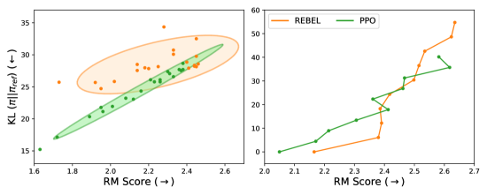
Figure 2: Plot of Reward vs KL-Divergence for 2.8B REBEL and PPO. We evaluate the models across the entire test set every 100 steps for 2,000 steps. Left: each point represents the average reward score and KL-divergence for a specific time step; the eclipse represents the confidence interval with 2 standard deviations. Right: we divide the KL distribution at the 2,000-step into $10$ bins with equal size and average the corresponding RM scores in each bin.

Table 1 presents a comparison between REBEL and SFT, PPO, and DPO for 1.4B and 2.8B models trained with LoRA. We calculate the KL-divergence (KL($\pi||\pi_{ref}$)) using the SFT policy of the corresponding size as the reference for all models. Notably, REBEL outperforms all the baselines on RM score across all model sizes with a slightly larger KL than PPO. In addition, REBEL achieves the highest winrate under GPT4 when evaluated against human references, indicating the benefit of regressing the relative rewards. Example generations of 2.8B REBEL are included in Appendix E. We also perform full-parameter training for 6.9B models and the winrates are shown in Table 2. We can observe that REBEL still outperforms all of the baselines while REBEL, PPO, and RLOO ($k=4$) have comparable performances (but we will soon show in the next section that REBEL is more tractable in computation and memory than PPO and RLOO with $k=4$). An ablation analysis on parameter $\eta$ is in Appendix F.

The trade-off between the reward model score and KL-divergence is shown in Figure 2. We evaluate the 2.8B REBEL and PPO every 400 gradient updates during training for 8,000 updates. The sample complexity of each update is held constant across both algorithms for fair comparison. For the left plot, each point represents the average divergence and score over the entire test set, and the eclipse represents the confidence interval with 2 standard deviations. As observed previously, PPO exhibits lower divergence, whereas REBEL shows higher divergence but is capable of achieving larger RM scores. Notably, towards the end of the training (going to the right part of the plot), REBEL and PPO have similar KL and RM scores. For the right plot in Figure 2, we analyze a single checkpoint for each algorithm at the end of training. For each algorithm, we group every generation from the test set by its KL distribution into $10$ equally sized bins and calculate the average of the corresponding RM score for each bin. We can see that REBEL achieves higher RM scores for generations with small divergence while requiring larger divergence for generations with the highest scores.

5.1.2 Runtime & Memory Analysis

We analyze the runtime and peak memory usage for 2.8B models using PPO, DPO, RLOO, and REBEL. The runtime includes both the generation time and the time required for policy updates. Both runtime and peak memory usage are measured on A6000 GPUs using the same hyperparameters detailed in Appendix D.2. The methods in the plots are arranged in ascending order based on winrates. To the right of the dashed line, PPO, RLOO ($k=4$), and REBEL have the highest winrates, which are comparable among them.

While DPO and REINFORCE require less time and memory, their performance does not match up to REBEL, as discussed in Section 5.1.1. RLOO ($k=2$) has similar runtime and memory usage as REBEL since we set $\mu=\pi_{t}$, making REBEL also generate twice per prompt. However, RLOO ($k=2$) has worse performance than REBEL. Compared to PPO and RLOO ($k=4$), REBEL demonstrates shorter runtimes and lower peak memory usage. PPO is slow and requires more memory because it needs to update both two networks: policy network and value network. RLOO ($k=4$) requires generating 4 responses per prompt which makes it slow and less memory efficient. Compared to the two baselines PPO and RLOO ($k=4$) that achieve similar winrates as REBEL, we see that REBEL is more computationally tractable. REBEL is also noticeably simpler to implement than PPO since it does not learn value networks or compute the advantage estimation.

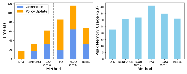
Figure 3: Plot of runtime and memory usage for DPO, REINFORCE, RLOO, PPO, and REBEL. The runtime includes both time for generation and policy update for each batch. Runtime and memory usage are measured on A6000 GPUs. Baselines on the left-hand side of the dashed line have lower winrates. Methods on the right-hand side of the dashed line have similar winrates to REBEL, but REBEL is noticeably more computationally tractable and memory efficient than PPO and RLOO ($k=4$).

5.2 Image Generation

We also consider the setting of image generation, where, given a consistency model (Song et al., 2023a) and a target reward function, we seek to train the consistency model to output images which garner a higher reward. Specifically, we compare REBEL and PPO under the RLCM framework (Oertell et al., 2024).

Baselines:

We compare REBEL to a clipped, policy gradient objective (Black et al., 2023; Fan et al., 2024; Oertell et al., 2024) with the aim to optimize aesthetic quality to obtain high reward from the LAION aesthetic score predictor (Schuhmann, 2022). This baseline does not use critics or GAE for advantage estimates. However, the clipping objective is clearly motivated by PPO, and thus, we simply name this baseline as PPO in this section.

Dataset:

We use 45 common animals as generation prompts similar to Black et al. (2023); Oertell et al. (2024).

Models:

We use the latent consistency model (Luo et al., 2023) distillation of the Dreamshaper v7 model, a finetune of stable diffusion (Rombach et al., 2021).

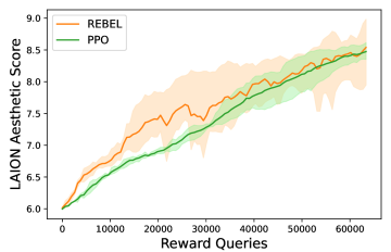
Figure 4: Learning curves as a function of reward queries to the LAION aesthetic predictor. We report inter-quartile means (IQM) with 95% confidence intervals (CIs) across three seeds for both REBEL and PPO. The CIs were calculated with percentile bootstrap with stratified sampling over three random seeds.

Evaluation:

We evaluate PPO and REBEL on its reward under the LAION aesthetic reward model for an equal number of reward queries/samples generated and an equal number of gradient updates. The aesthetic predictor is trained to predict human-labeled scores of images on a scale of 1 to 10. Images that tend to have the highest reward are artwork. Following the recommendations of Agarwal et al. (2021b), we report the inter-quartile mean with 95% confidence intervals for our reported results across three random seeds.

5.3 Quality Analysis

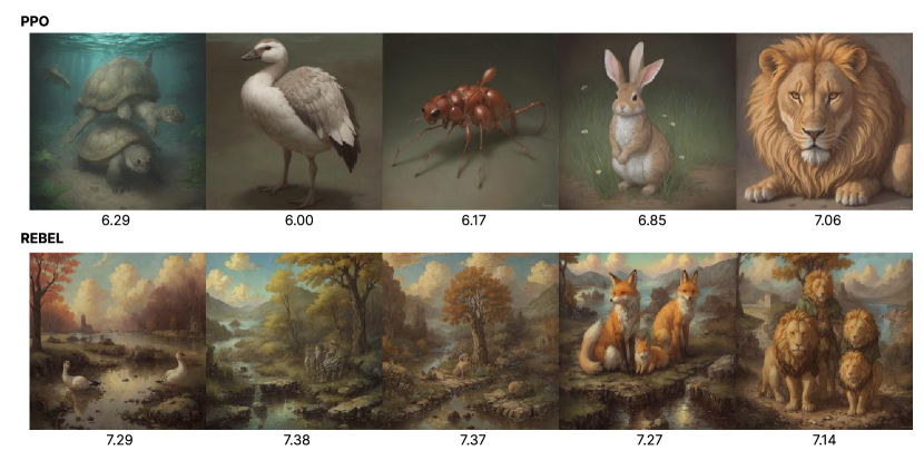
Figure 5: Generated images using PPO and REBEL during an intermediate checkpoint. We note that at the same number of epochs, REBEL observes a higher reward under the reward model. This can further be seen by the more diverse background of images generated from REBEL with less training time.

Figure 4 shows REBEL optimizes the consistency model faster during the beginning of training but eventually achieves similar performance to that of PPO. For our experiments, we tuned both batch size and learning rate for our algorithms, testing batch sizes of $[4,8,16]$ per gpu and learning rates $[1\text{e}-4,3\text{e}-4,6\text{e}-4,1\text{e}-3]$. Note, the main difference in implementation between PPO and REBEL is the replacement of the clipped PPO objective with our regression objective.

Qualitatively, we observe that eventually, both PPO and REBEL start to generate good-looking images but ignore the text prompt entirely. However, from just optimizing the reward function perspective, this behavior is not surprising since the objective does not encourage the maintenance of the consistency between the text prompt and the generated image. To maximize LAION-predicted aesthetic quality, both REBEL and PPO transform a model that produces plain images into one that produces artistic drawings. We found across multiple seeds that REBEL produced lush backgrounds when compared to PPO’s generations. Please see Appendix E.2 for more examples of generated images.

6 Related Work

Policy Gradients. Policy gradient (PG) methods (Nemirovskij and Yudin, 1983; Williams, 1992; Sutton et al., 1999; Konda and Tsitsiklis, 1999; Kakade, 2001; Schulman et al., 2017) are a prominent class of RL algorithms due to their direct, gradient-based policy optimization, robustness to model mis-specification (Agarwal et al., 2020), and scalability to modern AI applications from fine-tuning LLMs (Stiennon et al., 2022) to optimizing text-to-image generators (Oertell et al., 2024).

Broadly speaking, we can taxonomize PG methods into two families. The first family is based on REINFORCE (Williams, 1992) and often includes variance reduction techniques (Kool et al., 2019; Richter et al., 2020; Zhu et al., 2023). While prior work by Ahmadian et al. (2024) has shown that REINFORCE-based approaches can outperform more complex RL algorithms like PPO on LLM fine-tuning tasks like TL;DR, we find that a properly optimized version of PPO still out-performs a REINFORCE baseline. The second family is adaptive PG techniques that precondition the policy gradient (usually with the inverse of the Fisher Information Matrix) to ensure it is covariant to re-parameterizations of the policy, which include NPG (Kakade, 2001; Bagnell and Schneider, 2003) and its practical approximations like TRPO (Schulman et al., 2015a) and PPO (Schulman et al., 2017). Intuitively, the preconditioning ensures that we make small changes in terms of action distributions, rather than in terms of the actual policy parameters, leading to faster and more stable convergence. Unfortunately, computing and then inverting the Fisher Information Matrix is computationally intensive and therefore we often resort to approximations in practice, as done in TRPO. However, these approximations are still difficult to apply to large-scale generative models, necessitating even coarser approximations like PPO. In contrast, REBEL does not need any such approximations to be implemented at scale, giving us a much closer connection between theory and practice.

Reward Regression. The heart of REBEL is a novel reduction from RL to iterative squared loss regression. While using regression to fit either the reward (Peters and Schaal, 2007) or the value (Peng et al., 2019) targets which are then used to extract a policy have previously been explored, our method instead takes a page from DPO (Rafailov et al., 2023) to implicitly parameterize the reward regressor in terms of the policy. This collapses the two stage procedure of prior methods into a single regression step.

Preference Fine-Tuning (PFT) of Generative Models. RL has attracted renewed interest due to its central role in “aligning” language models – i.e., adapting their distribution of prompt completions towards the set of responses preferred by human raters.

One family of techniques for PFT, often referred to as Reinforcement Learning from Human Feedback (RLHF) involves first fitting a reward model (i.e. a classifier) to the human preference data and then using this model to provide reward values to a downstream RL algorithm (often PPO) (Christiano et al., 2017; Ziegler et al., 2020). LLMs fine-tuned by this procedure include GPT-N (OpenAI, 2023), Claude-N (Anthropic, 2024), and Llama-N (Meta, 2024). Similar approaches have proved beneficial for tasks like summarization (Stiennon et al., 2022), question answering (Nakano et al., 2022), text-to-image generation (Lee et al., 2023), and instruction following (Ouyang et al., 2022).

Another family of techniques for PFT essentially treats the problem as supervised learning and uses a variety of ranking loss functions. It includes DPO (Rafailov et al., 2023), IPO (Azar et al., 2023), and KTO (Ethayarajh et al., 2023). These techniques are simpler to implement as they remove components like an explicit reward model, value network, and on-policy training from the standard RLHF setup. However, recent work finds their performance to be lesser than that of on-policy methods (Lambert et al., 2024; Tajwar et al., 2024), which agrees with our findings. This is perhaps caused by their lack of interaction during training, leading to the well-known covariate shift/compounding error issue (Ross et al., 2011; Swamy et al., 2021) and the associated lower levels of performance.

The third family of PFT techniques combines elements from the previous two: it involves running an offline algorithm iteratively, collecting on-policy preference feedback from either a supervisor model (Rosset et al., 2024; Xiong et al., 2024; Guo et al., 2024) or from a preference model fit on human data (Calandriello et al., 2024). All of these approaches can be considered instantiations of the general SPO reduction proposed by Swamy et al. (2024), which itself can be thought of as a preference-based variant of DAgger (Ross et al., 2011). Recent work by Tajwar et al. (2024) confirms the empirical strength of these techniques. Our approach fits best into this family of techniques – we also iteratively update our model by solving a sequence of supervised learning problems over on-policy datasets. However, REBEL comes with several key differentiating factors from the prior work. First, we can run REBEL with datasets consisting of a mixture of on-policy and off-policy data with strong guarantees, enabling hybrid training, as previously explored in the RL (Song et al., 2023b; Ball et al., 2023; Zhou et al., 2023) and inverse RL (Ren et al., 2024) literature. Second, unlike all of the aforementioned works that regularize to the initial policy $\pi_{0}$ during updates, we perform conservative updates by regularizing $\pi_{t+1}$ to $\pi_{t}$. Thus, for the prior work, it is difficult to prove convergence or monotonic improvement as the current policy can just bounce around a ball centered at $\pi_{0}$, a well-known issue in the theory of approximate policy iteration (Kakade and Langford, 2002; Munos, 2003). In contrast, by incorporating the prior policy’s probabilities into our regression problem, we are able to prove stronger guarantees for REBEL.

7 Summary and Future Work

In summary, we propose REBEL, an RL algorithm that reduces the problem of RL to solving a sequence of relative reward regression problems on iteratively collected datasets. In contrast to policy gradient approaches that require additional networks and heuristics like clipping to ensure optimization stability, REBEL requires that we can drive down training error on a least squares problem. This makes it strikingly simple to implement and scale. In theory, REBEL matches the best guarantees we have for RL algorithms in the agnostic setting, while in practice, REBEL is able to match and sometimes outperform methods that are far more complex to implement or expensive to run across both language modeling and guided image generation tasks.

There are several open questions raised by our work. The first is whether using a loss function other than square loss (e.g. log loss or cross-entropy) could lead to better performance in practice (Farebrother et al., 2024) or tighter bounds (e.g. first-order / gap-dependent) in theory (Foster and Krishnamurthy, 2021; Wang et al., 2023a, 2024). The second is whether, in the general (i.e. non-utility-based) preference setting, the coverage condition assumed in our analysis is necessary – we conjecture it is. Relatedly, it would be interesting to explore whether using preference (rather than reward) models to provide supervision for REBEL replicates the performance improvements reported by Swamy et al. (2024); Munos et al. (2023). Third, while we focus primarily on the bandit setting in the preceding sections, it would be interesting to consider the more general RL setting and explore how offline datasets can be used to improve the efficiency of policy optimization via techniques like resets (Bagnell et al., 2003; Ross and Bagnell, 2014; Swamy et al., 2023; Chang et al., 2023, 2024).

Appendix A Proof of Claim 1

We prove claim 1 in this section. We start from deriving the Fisher information matrix.

$$F_{t} :=\frac{1}{\eta^{2}}\mathbb{E}_{x,y\sim\pi_{t},y^{\prime}\sim\mu}\left(\nabla_{\theta}\ln\pi_{\theta_{t}}(y|x)-\nabla_{\theta}\ln\pi_{\theta_{t}}(y^{\prime}|x)\right)\left(\nabla_{\theta}\ln\pi_{\theta_{t}}(y|x)-\nabla_{\theta}\ln\pi_{\theta_{t}}(y^{\prime}|x)\right)^{\top}$$

$$=\frac{2}{\eta^{2}}\mathbb{E}_{x,y\sim\pi_{mix}}\nabla_{\theta}\ln\pi_{\theta_{t}}(y|x)\nabla_{\theta}\ln\pi_{\theta_{t}}(y|x)^{\top}$$

where the last equality uses the fact that cross terms from completing the square are zero. Now recall Eq. 13 which is a ordinarly least square regression problem. The minimum norm solution of the least square regression problem is:

$$\delta =(\eta/2)\tilde{F}_{t}^{\dagger}\left(\mathbb{E}_{x,y\sim\pi_{t},y^{\prime}\sim\mu}\left(\nabla_{\theta}\ln\pi_{\theta_{t}}(y|x)-\nabla_{\theta}\ln\pi_{\theta_{t}}(y^{\prime}|x)\right)\left(r(x,y)-r(x,y^{\prime})\right)\right)$$

$$=(\eta/2)\tilde{F}_{t}^{\dagger}\Big{(}\mathbb{E}_{x,y\sim\pi_{t}}\left[\nabla_{\theta}\ln\pi_{\theta_{t}}(y|x)r(x,y)\right]+\mathbb{E}_{x,y^{\prime}\sim\mu}\left[\nabla_{\theta}\ln\pi_{\theta_{t}}(y^{\prime}|x)r(x,y^{\prime})\right]$$

$$\quad\quad-\mathbb{E}_{x,y\sim\pi_{t}y^{\prime}\sim\mu}\nabla_{\theta}\ln\pi_{\theta_{t}}(y^{\prime}|x)r(x,y)\Big{)}$$

$$=(\eta/2)\tilde{F}_{t}^{\dagger}\Big{(}\mathbb{E}_{x,y\sim\pi_{t}}\left[\nabla_{\theta}\ln\pi_{\theta_{t}}(y|x)[r(x,y)-\mathbb{E}_{y^{\prime}\sim\pi_{t}(\cdot|x)}r(x,y^{\prime})\right]$$

$$\qquad\qquad+\mathbb{E}_{x,y\sim\mu}\left[\nabla_{\theta}\ln\pi_{\theta_{t}}(y|x)[r(x,y)-\mathbb{E}_{y^{\prime}\sim\pi_{t}(\cdot|x)}r(x,y^{\prime})\right]\Big{)}$$

$$=(\eta)\tilde{F}_{t}^{\dagger}\left(\mathbb{E}_{x,y\sim(\pi_{t}+\mu)/2}\left[\nabla_{\theta}\ln\pi_{\theta_{t}}(y|x)[A^{\pi_{t}}(x,y)\right]\right)$$

where we again use the fact that $\mathbb{E}_{y\sim\pi_{\theta_{t}}(\cdot|x)}\nabla_{\theta}\ln\pi_{\theta_{t}}(y|x)g(x)=0$ for any function $g(x)$, and we define Advantage $A^{\pi}(x,y):=r(x,y)-\mathbb{E}_{y^{\prime}\sim\pi(\cdot|x)}r(x,y^{\prime})$.

Appendix B Proof of Theorem 1

In this section, we provide the proof of theorem 1. For notation simplicity, throughout the proof, we denote $\pi_{t}$ for $\pi_{\theta_{t}}$, and define $f_{t}(x,y):=\frac{1}{\eta}\ln\frac{\pi_{t+1}(y|x)}{\pi_{t}(y|x)}$.

The following lemma shows that the learned function $f_{t}$ can predict reward $r$ well under both $\pi_{t}$ and $\mu$ up to terms that are $y$-independent.

Lemma 1.

Consider any $t\in[T]$. Define $\Delta(x,y)=f_{t}(x,y)-r(x,y)$. Define $\Delta_{\pi_{t}}(x)=\mathbb{E}_{y\sim\pi_{t}(\cdot|x)}\Delta(x,y)$ and $\Delta_{\mu}(x)=\mathbb{E}_{y\sim\mu(\cdot|x)}\Delta(x,y)$. Under assumption 1, for all $t$, we have the following:

$$\mathbb{E}_{x,y\sim\pi_{t}(\cdot|x)}\left(f_{t}(x,y)-r(x,y)-\Delta_{\pi_{t}}(x)\right)^{2}\leq\epsilon,$$ (16)

$$\mathbb{E}_{x,y\sim\mu(\cdot|x)}\left(f_{t}(x,y)-r(x,y)-\Delta_{\mu}(x)\right)^{2}\leq\epsilon,$$ (17)

$$\mathbb{E}_{x}\left(\Delta_{\pi_{t}}(x)-\Delta_{\mu}(x)\right)^{2}\leq\epsilon.$$ (18)

Proof.

From assumption 1, we have:

$$\mathbb{E}_{x,y_{1}\sim\pi_{t},y_{2}\sim\mu}\left(f_{t}(x,y_{1})-\Delta_{\pi_{t}}(x)-r(x,y_{1})-\left(f_{t}(x,y_{2})-\Delta_{\mu}(x)-r(x,y_{2})\right)+\Delta_{\pi_{t}}(x)-\Delta_{\mu}(x)\right)^{2}$$

$$=\mathbb{E}_{x,y_{1}\sim\pi_{t}}\left(f_{t}(x,y_{1})-\Delta_{\pi_{t}}(x)-r(x,y_{1})\right)^{2}+\mathbb{E}_{x,y_{2}\sim\mu}\left(f_{t}(x,y_{2})-\Delta_{\mu}(x)-r(x,y_{2})\right)^{2}$$

$$-2\mathbb{E}_{x,y_{1}\sim\pi_{t},y_{2}\sim\mu}\left(f_{t}(x,y_{1})-\Delta_{\pi_{t}}(x)-r(x,y_{1})\right)\left(f_{t}(x,y_{2})-\Delta_{\mu}(x)-r(x,y_{2})\right)$$

$$+2\mathbb{E}_{x,y_{1}\sim\pi_{t}}\left(f_{t}(x,y_{1})-\Delta_{\pi_{t}}(x)-r(x,y_{1})\right)(\Delta_{\pi_{t}}(x)-\Delta_{\mu}(x))$$

$$-2\mathbb{E}_{x,y_{2}\sim\pi_{t}}\left(f_{t}(x,y_{2})-\Delta_{\mu}(x)-r(x,y_{2})\right)(\Delta_{\pi_{t}}(x)-\Delta_{\mu}(x))+\mathbb{E}_{x}(\Delta_{1}(x)-\Delta_{2}(x))^{2}$$

$$=\mathbb{E}_{x,y_{1}\sim\pi_{t}}\left(f_{t}(x,y_{1})-\Delta_{\pi_{t}}(x)-r(x,y_{1})\right)^{2}+\mathbb{E}_{x,y_{2}\sim\mu}\left(f_{t}(x,y_{2})-\Delta_{\mu}(x)-r(x,y_{2})\right)^{2}$$

$$\qquad+\mathbb{E}_{x}(\Delta_{\pi_{t}}(x)-\Delta_{\mu}(x))^{2}\leq\epsilon.$$

In the above, we first complete the square, and then we only keep terms that are not necessarily zero. Since all the remaining three terms are non-negative, this concludes the proof. ∎

By the definition of $f_{t}$, we have $\Delta(x,y)=\frac{1}{\eta}\ln\frac{\pi_{t+1}(y|x)}{\pi_{t}(y|x)}-r(x,y)$. Taking $\exp$ on both sides, we get:

$$\forall x,y:\;\pi_{t+1}(y|x)=\pi_{t}(y|x)\exp\left(\eta(r(x,y)+\Delta(x,y))\right)=\frac{\pi_{t}(y|x)\exp(\eta(r(x,y)+\Delta(x,y)-\Delta_{\mu}(x)))}{\exp(-\eta\Delta_{\mu}(x))}$$

Denote $g_{t}(x,y):=r(x,y)+\Delta(x,y)-\Delta_{\mu}(x)$, and the advantage $A_{t}(x,y)=g_{t}(x,y)-\mathbb{E}_{y^{\prime}\sim\pi_{t}(\cdot|x)}g_{t}(x,y^{\prime})$. We can rewrite the above update rule as:

$$\forall x,y:\;\pi_{t+1}(y|x)\propto\pi_{t}(y|x)\exp(\eta A_{t}(x,y))$$ (19)

In other words, the algorithm can be understood as running MD on the sequence of $A_{t}$ for $t=0$ to $T-1$. The following lemma is the standard MD regret lemma.

Lemma 2.

Assume $\max_{x,y,t}|A_{t}(x,y)|\leq A\in\mathbb{R}^{+}$, and $\pi_{0}(\cdot|x)$ is uniform over $\mathcal{Y}$. Then with $\eta=\sqrt{\ln(|\mathcal{Y}|)/(A^{2}T)}$, for the sequence of policies computed by REBEL, we have:

$$\forall\pi,x:\;\sum_{t=0}^{T-1}\mathbb{E}_{y\sim\pi(\cdot|x)}A_{t}(x,y)\leq 2A\sqrt{\ln(|\mathcal{Y}|)T}.$$

Proof.

For completeness, we provide the proof here. Start with $\pi_{t+1}(y|x)=\pi_{t}(y|x)\exp(\eta A_{t}(x,y))/Z_{t}(x)$ where $Z_{t}(x)$ is the normalization constant, taking log on both sides, and add $\mathbb{E}_{y\sim\pi(\cdot|x)}$, we have:

$$-\text{KL}(\pi(\cdot|x)||\pi_{t+1}(\cdot|x))=-\text{KL}(\pi(\cdot|x)||\pi_{t}(\cdot|x))+\eta\mathbb{E}_{y\sim\pi(\cdot|x)}A_{t}(x,y)-\mathbb{E}_{y\sim\pi(\cdot|x)}\ln Z_{t}(x).$$

Rearrange terms, we get:

$$-\text{KL}(\pi(\cdot|x)||\pi_{t}(\cdot|x))+\text{KL}(\pi(\cdot|x)||\pi_{t+1}(\cdot|x)=\mathbb{E}_{y\sim\pi(\cdot|x)}\left[-\eta A_{t}(x,y)+\ln Z_{t}(x)\right]$$

For $\ln Z_{t}(x)$, using the condition that $\eta\leq 1/A$, we have $\eta A_{t}(x,y)\leq 1$, which allows us to use the inequality $\exp(x)\leq 1+x+x^{2}$ for any $x\leq 1$, which lead to the following inequality:

$$\ln Z_{t}(x) =\ln\left(\mathbb{E}_{y\sim\pi(\cdot|x)}\exp(\eta A_{t}(x,y))\right)$$

$$\leq\ln\left(\sum_{y}\pi_{t}(y|x)\left(1+\eta A_{t}(x,y)+\eta^{2}A_{t}(x,y)^{2}\right)\right)$$

$$\leq\ln\left(1+0+\eta^{2}A^{2}\right)\leq\eta^{2}A^{2},$$

where the last inequality uses $\ln(1+x)\leq x$, and we used the fact that $\mathbb{E}_{y\sim\pi_{t}(x)}A_{t}(x,y)=0$ due to the definition of advantage $A_{t}$. Thus, we have:

$$-\text{KL}(\pi(\cdot|x)||\pi_{t}(\cdot|x))+\text{KL}(\pi(\cdot|x)||\pi_{t+1}(\cdot|x)\leq-\mathbb{E}_{y\sim\pi(\cdot|x)}[A_{t}(x,y)]+\eta^{2}A^{2}.$$

Sum over all iterations and do the telescoping sum, we get:

$$\sum_{t=0}^{T-1}\mathbb{E}_{y\sim\pi(\cdot|x)}A_{t}(x,y)\leq\text{KL}(\pi(\cdot|x)||\pi_{0}(\cdot|x))/\eta+T\eta A^{2}\leq\ln(|\mathcal{Y}|)/\eta+T\eta A^{2}.$$

With $\eta=\sqrt{\ln(|\mathcal{Y}|)/(A^{2}T)}$, we conclude the proof. ∎

With the above, now we are ready to conclude the proof of the main theorem.

Proof of Theorem 1.

Consider a comparator policy $\pi^{*}$. We start with the performance difference between $\pi^{*}$ and the uniform mixture policy $\bar{\pi}:=\sum_{t=0}^{T-1}\pi_{t}/T$:

$$\frac{1}{T}\sum_{t=0}^{T-1}\left(\mathbb{E}_{x,y\sim\pi^{*}(\cdot|x)}r(x,y)-\mathbb{E}_{x,y\sim\pi_{t}(\cdot|x)}r(x,y)\right)=\frac{1}{T}\sum_{t=0}^{T-1}\mathbb{E}_{x,y\sim\pi^{*}(\cdot|x)}\left(A^{\pi_{t}}(x,y)\right),$$

where we define the real advantage $A^{\pi_{t}}(x,y):=r(x,y)-\mathbb{E}_{y\sim\pi_{t}(\cdot|x)}r(x,y)$. Continue, we have:

$$\frac{1}{T}\sum_{t=0}^{T-1}\mathbb{E}_{x,y\sim\pi^{*}(\cdot|x)}\left(A^{\pi_{t}}(x,y)\right)$$

$$=\frac{1}{T}\sum_{t=0}^{T-1}\mathbb{E}_{x,y\sim\pi^{*}(\cdot|x)}\left(A_{t}(x,y)\right)+\frac{1}{T}\sum_{t=0}^{T-1}\mathbb{E}_{x,y\sim\pi^{*}(\cdot|x)}\left(A^{\pi_{t}}(x,y)-A_{t}(x,y)\right)$$

$$\leq 2A\sqrt{\frac{\ln(|\mathcal{Y}|)}{T}}+\frac{1}{T}\sum_{t=0}^{T-1}\sqrt{\mathbb{E}_{x}\mathbb{E}_{y\sim\pi^{*}(\cdot|x)}(A^{\pi_{t}}(x,y)-A_{t}(x,y))^{2}}$$

where the last inequality uses Lemma 2. We now just need to bound $\mathbb{E}_{y\sim\pi^{*}(\cdot|x)}(A^{\pi_{t}}(x,y)-A_{t}(x,y))^{2}$.

$$\mathbb{E}_{x}\mathbb{E}_{y\sim\pi^{*}(\cdot|x)}(A^{\pi_{t}}(x,y)-A_{t}(x,y))^{2} =\mathbb{E}_{x}\mathbb{E}_{y\sim\mu(\cdot|x)}\frac{\pi^{*}(y|x)}{\mu(y|x)}(A^{\pi_{t}}(x,y)-A_{t}(x,y))^{2}$$

$$\leq C_{\pi^{*}}\mathbb{E}_{x,y\sim\mu(\cdot|x)}(A^{\pi_{t}}(x,y)-A_{t}(x,y))^{2}$$

where the last inequality uses the definition of concentrability coefficient $C_{\pi^{*}}$. We now bound $\mathbb{E}_{x,y\sim\mu(\cdot|x)}(A^{\pi_{t}}(x,y)-A_{t}(x,y))^{2}$. Recall the definiton of $A_{t}$ from Lemma 2.

$$\mathbb{E}_{x,y\sim\mu(\cdot|x)}(A^{\pi_{t}}(x,y)-A_{t}(x,y))^{2}$$

$$=\mathbb{E}_{x,y\sim\mu(\cdot|x)}(r(x,y)-\mathbb{E}_{y^{\prime}\sim\pi_{t}(\cdot|x)}r(x,y^{\prime})-g_{t}(x,y)+\mathbb{E}_{y^{\prime}\sim\pi_{t}(\cdot|x)}g_{t}(x,y^{\prime}))^{2}$$

$$\leq 2\mathbb{E}_{x,y\sim\mu(\cdot|x)}\left(r(x,y)-g_{t}(x,y)\right)^{2}+2\mathbb{E}_{x}\mathbb{E}_{y^{\prime}\sim\pi_{t}(\cdot|x)}\left(r(x,y^{\prime})-g_{t}(x,y^{\prime})\right)^{2}$$

Recall the $g_{t}(x,y)=r(x,y)+\Delta(x,y)-\Delta_{\mu}(x)$, and from Lemma 1, we can see that

$$\mathbb{E}_{x,y\sim\mu(\cdot|x)}(r(x,y)-g_{t}(x,y))^{2}=\mathbb{E}_{x,y\sim\mu(\cdot|x)}(\Delta(x,y)-\Delta_{\mu}(x))^{2}\leq\epsilon.$$

For $\mathbb{E}_{x}\mathbb{E}_{y^{\prime}\sim\pi_{t}(\cdot|x)}\left(r(x,y^{\prime})-g_{t}(x,y^{\prime})\right)^{2}$, we have:

$$\mathbb{E}_{x} \mathbb{E}_{y^{\prime}\sim\pi_{t}(\cdot|x)}\left(r(x,y^{\prime})-g_{t}(x,y^{\prime})\right)^{2}=\mathbb{E}_{x}\mathbb{E}_{y^{\prime}\sim\pi_{t}(\cdot|x)}\left(\Delta(x,y^{\prime})-\Delta_{\mu}(x)\right)^{2}$$

$$=\mathbb{E}_{x}\mathbb{E}_{y^{\prime}\sim\pi_{t}(\cdot|x)}\left(\Delta(x,y^{\prime})-\Delta_{\pi_{t}}(x)+\Delta_{\pi_{t}}(x)-\Delta_{\mu}(x)\right)^{2}$$

$$\leq 2\mathbb{E}_{x}\mathbb{E}_{y^{\prime}\sim\pi_{t}(\cdot|x)}\left(\Delta(x,y^{\prime})-\Delta_{\pi_{t}}(x)\right)^{2}+2\mathbb{E}_{x}\left(\Delta_{\pi_{t}}(x)-\Delta_{\mu}(x)\right)^{2}\leq 4\epsilon,$$

where the last inequality uses Lemma 1 again. Combine things together, we can conclude that:

$$\mathbb{E}_{x}\mathbb{E}_{y\sim\pi^{*}(\cdot|x)}(A^{\pi_{t}}(x,y)-A_{t}(x,y))^{2}\leq C_{\pi^{*}}(10\epsilon).$$

Finally, for the regret, we can conclude:

$$\frac{1}{T}\sum_{t=0}^{T-1}\mathbb{E}_{x,y\sim\pi^{*}(\cdot|x)}\left(A^{\pi_{t}}(x,y)\right)\leq 2A\sqrt{\frac{\ln|\mathcal{Y}|}{T}}+\frac{1}{T}\sum_{t}\sqrt{C_{\pi^{*}}10\epsilon}=2A\sqrt{\frac{\ln|\mathcal{Y}|}{T}}+\sqrt{C_{\pi^{*}}10\epsilon}.$$

∎

Appendix C Proof of Theorem 2

Recall that $r_{t}(x,y)=l(x,y,\pi_{t})$. Let us define $\Delta^{t}(x,y):=f_{t}(x,y)-r_{t}(x,y)$, $\Delta^{t}_{\pi_{t}}(x):=\mathbb{E}_{y\sim\pi_{t}(\cdot|x)}\Delta^{t}(x,y)$ and $\Delta^{t}_{\mu}(x):=\mathbb{E}_{y\sim\mu(\cdot|x)}\Delta^{t}(x,y)$. Then following the same arguments in Lemma 1, we have

$$\mathbb{E}_{x\sim\rho,y\sim\pi_{t}(\cdot|x)}\left[\left(f_{t}(x,y)-r_{t}(x,y)-\Delta^{t}_{\pi_{t}}(x)\right)^{2}\right]\leq\epsilon,$$ (20)

$$\mathbb{E}_{x\sim\rho,y\sim\mu(\cdot|x)}\left[\left(f_{t}(x,y)-r_{t}(x,y)-\Delta^{t}_{\mu}(x)\right)^{2}\right]\leq\epsilon,$$ (21)

$$\mathbb{E}_{x\sim\rho}\left[\left(\Delta^{t}_{\pi_{t}}(x)-\Delta^{t}_{\mu}(x)\right)^{2}\right]\leq\epsilon.$$ (22)

With slight abuse of the notation, We also use $g_{t}$ and $A_{t}(x,y)$ to denote $r_{t}(x,y)+\Delta^{t}(x,y)-\Delta^{t}_{\mu}(x,y)$ and $g_{t}(x,y)-\mathbb{E}_{y^{\prime}\sim\pi_{t}(\cdot|x)}g_{t}(x,y^{\prime})$. Then following the same arguments in Lemma 2,

$$\forall\pi,x:\;\sum_{t=0}^{T-1}\mathbb{E}_{y\sim\pi(\cdot|x)}A_{t}(x,y)\leq 2A\sqrt{\ln(|\mathcal{Y}|)T}.$$ (23)

Note that we have

$$\max_{\pi}l(\pi,\widehat{\pi})=\max_{\pi}\frac{1}{T}\sum_{t=1}^{T}l(\pi,\pi_{t})$$

$$\qquad=\max_{\pi}\frac{1}{T}\sum_{t=1}^{T}\mathbb{E}_{x\sim\rho,y\sim\pi(\cdot|x)}[r_{t}(x,y)]=\max_{\pi}\frac{1}{T}\sum_{t=1}^{T}\mathbb{E}_{x\sim\rho,y\sim\pi(\cdot|x)}[A^{t,\pi_{t}}(x,y)],$$

where $A^{t,\pi_{t}}:=r_{t}(x,y)-\mathbb{E}_{y\sim\pi_{t}(\cdot|x)}[r_{t}(x,y)]$. The last step is due to the skew symmetry of $l$, i.e., $\mathbb{E}_{y\sim\pi_{t}(\cdot|x)}[r_{t}(x,y)]=l(x,\pi_{t},\pi_{t})=0$. Then by following the same arguments in the proof of Theorem 1, with (20)(21)(22)(23), we have for any policy $\pi$,

$$\frac{1}{T}\sum_{t=0}^{T-1}\mathbb{E}_{x\sim\rho,y\sim\pi(\cdot|x)}\left(A^{t,\pi_{t}}(x,y)\right)\leq 2A\sqrt{\frac{\ln|\mathcal{Y}|}{T}}+\sqrt{10C_{\mu\to\pi}\epsilon}.$$

This implies that

$$\max_{\pi}l(\pi,\widehat{\pi})\leq\max_{\pi}\left(2A\sqrt{\frac{\ln|\mathcal{Y}|}{T}}+\sqrt{10C_{\mu\to\pi}\epsilon}\right)\leq 2A\sqrt{\frac{\ln|\mathcal{Y}|}{T}}+\sqrt{10C_{\mu}\epsilon}.$$

Note that due to the skew symmetry of $l$, we have

$$\min_{\pi}l(\widehat{\pi},\pi)=\min_{\pi}\mathbb{E}_{x\sim\rho,y\sim\widehat{\pi}(\cdot|x),y^{\prime}\sim\pi(\cdot|x)}\left[l(x,y,y^{\prime})\right]=-\max_{\pi}\mathbb{E}_{x\sim\rho,y\sim\widehat{\pi}(\cdot|x),y^{\prime}\sim\pi(\cdot|x)}\left[-l(x,y,y^{\prime})\right]$$

$$\qquad=-\max_{\pi}\mathbb{E}_{x\sim\rho,y\sim\pi(\cdot|x),y^{\prime}\sim\widehat{\pi}(\cdot|x)}\left[l(x,y,y^{\prime})\right]=-\max_{\pi}l(\pi,\widehat{\pi})\geq-2A\sqrt{\frac{\ln|\mathcal{Y}|}{T}}-\sqrt{10C_{\mu}\epsilon}.$$

Therefore we have

$$\mathsf{DG}(\widehat{\pi})\leq 4A\sqrt{\frac{\ln|\mathcal{Y}|}{T}}+2\sqrt{10C_{\mu}\epsilon}.$$

Appendix D Additional Experiment Details

D.1 Dataset Details

We present dataset details in Table 3.

Table 3: Dataset split, prompts, and maximum generation length

Dataset	Train/Val/Test	Prompt	Generation Length
Human Reference	117K/6.45K/6.55K	“TL;DR:”	53
Preference	92.9K/83.8K/-	“TL;DR:”	53

D.2 Hyperparameter Details

Parameter setting for TL;DR summarization Setting Parameters SFT & RM batch size: 64
learning rate: 3e-6 schedule: linear decay
train epochs: 1 PPO batch size: 512
learning rate: 3e-6
schedule: linear decay
train epochs: 1
num epochs: 4 discount factor: 1
gae $\lambda$: 0.95
clip ratio: 0.2
value function coeff: 0.1
kl coefficient: 0.05 DPO batch size: 64
learning rate: 3e-6
schedule: linear decay train epochs: 1
$\beta$: 0.05 REBEL batch size: 512
learning rate: 3e-6
schedule: linear decay
train epochs: 1 num epochs: 4
$\eta$: 1.0
kl coefficient: 0.05 LoRA Adapter
Config r: 1024
$\alpha$: 2048 dropout: 0.0
bias: False Generation sampling: true
top k: 0.0
top p: 1.0 min length: 53
max new tokens: 53
temperature: 0.1

D.3 Winrate Details

Below we show the prompt for winrate evaluation and an example evaluation from GPT4.

Prompt for Winrate Which of the following summaries does a better job of summarizing the most important points in the given forum post, without including unimportant or irrelevant details? Judge based on accuracy, coverage, and coherence.

### Post:
{{post}}

### Summary A:
{{summarya}}

### Summary B:
{{summaryb}}

### Instructions:
FIRST provide a one-sentence comparison of the two summaries, explaining which you prefer and why. SECOND, on a new line, state only “A” or “B” to indicate your choice. Your response should use the format:
Comparison: <one-sentence comparison and explanation >
Preferred: <“A” or “B”>

Example Evaluation from GPT4 Prompt SUBREDDIT: r/AskReddit

TITLE: How do you get someone out of your head?

POST: Hi,
I’m 22, and I have been with my girlfriend for 5 years now. We recently moved together. We’ve always loved each other intensely.

Problem, I recently started to have feelings for an other person (a friend). This person has had a boyfriend for now 3 years, and has absolutely no ideas. Those feelings were so strong, it was hard to hide them. After 2 months of me being distant and really sad, my girlfriend forced me to say what was bothering me. I’m not a good liar, and now she knows.

We decided to give us a week alone, I went to my parents.

Now, I’m completely lost. I keep on thinking about this person, and I hate that. I would like for those feelings to go away, to leave me alone. But I can’t.

What do I do? It’s been 3 months now, and I’m just desperate.

TL;DR: Reference
(Summary A) long relationship; fell in love with an other person; admitted it; would like it to disappear, though it doesn’t. REBEL
Generation
(Summary B) I recently started to have feelings for an other person (a friend). We decided to give us a week alone, I keep on thinking about that person, and I hate it. What do I do? Evaluation from GPT4 Comparison: Summary A is too brief and rather disjointed, while Summary B more accurately conveys the emotional conflict portrayed in the forum post in a coherent manner.
Preferred: B

Appendix E Example Generations

E.1 Summarization Generations

Prompt	SUBREDDIT: r/relationships TITLE: Me [18 M] with my college friend [19 F] about 1 month, I wanna hang out with her but I don’t have a car. POST: This is the link for an earlier thread I posted about her She basically doesn’t have any friends and will spend all her spring break at home playing video games. I wanna hang out with her, but both of us don’t have a car. I live with my grandma 10 minutes away from her house. Would it be weird to ask her to spend a day with us playing video games and eating pizza? Another thing I could do is ask her to go see a movie with me, but I would just meet her there since I’ll be going with a bike. Do you guys think it’s okay to do that? I also have 0 experience with girls. You can say this is the first girl in my life. TL;DR:
Generation	My college friend doesn’t have any friends and spends all her spring break at home playing video games. I wanna hang out with her but neither of us have a car. Do you think it’s okay to ask her to hang out?
Prompt	SUBREDDIT: r/AskReddit TITLE: Reddit, what kind of effect do you think that crime shows/movies might have in reducing the occurrence of thought-out, "intelligent" crime? POST: I had this thought a few days ago when watching an episode of NCIS and they did the usual "create a super high resolution image from a very low resolution image." I got to wondering how much of it is real and how much of it is fake (or, conversely, how much might be under-exaggerated). Based on these types of shows/movies (bank robbery, conning, etc.) where the bad guy nearly 100% of the time gets caught, only an idiot would think it would be a good idea to do any of this stuff, and from my [limited] knowledge of the general criminal, I’m under the impression that they are mainly uneducated people in dire situations (or psychopaths/mentally unstable.. but I’m thinking mostly with regards the heist type of crime – not assault or murder) that are driven to extreme lengths to make the "easy"/"quick" dollar. So I wondered, is it possible that these shows/movies that show the criminal, no matter how smart and creative, almost always getting caught could actually be (subconsciously or consciously) reducing the amount of more well thought through crime throughout the world? TL;DR:
Generation	I had this thought recently watching NCIS episode where criminals almost always get caught, is it possible that these crime shows/movies that show the criminal almost always getting caught could actually be (subconsciously or consciously) reducing the crime?

E.2 Image Generations

Appendix F Ablation Analysis

$\eta$	Winrate ($\uparrow$)	RM Score ($\uparrow$)	KL($\pi||\pi_{ref}$) ($\downarrow$)
0.3	55.5%	1.37	10.4
0.7	59.9%	1.60	14.2
1.0	70.3%	2.44	29.2
2.0	62.5%	1.76	16.9

Table 4: REBEL ablation of the key hyperparameter $\eta$ . The best-performing $\eta$ for each metric is highlighted in bold.

Just like DPO, tuning REBEL is much more straightforward than PPO since the only hyperparameter REBEL introduced is $\eta$. We investigate how sensitive REBEL is to learning rate $\eta$ in the loss. The results of ablation is shown in Table 4 with the same setting detailed in Appendix D.2 except for $\eta$. REBEL achieves the best performance when $\eta=1$, while increasing or decreasing $\eta$ leads to decreased performance. Our result here indicates that $\eta$ is an important hyperparameter that requires tuning for achieving a good performance.

Appendix G Regression Loss During Training

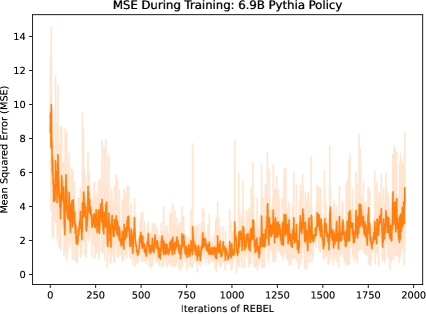
Figure 6: REBEL’s reward difference prediction error throughout training of our 6.9B parameter policy on the TL;DR task. The reward used for this task is unbounded with the range of values of the human labels in the validation set being $[-6.81,7.31]$. We plot both the smoothed values with a moving average and the loss vales at each iteration.

Figure 6 shows the observed loss or Eq. 9 that we observed when finetuning the 6.9B Pythia model on TL;DR. We see that REBEL minimizes the loss throughout training maintaining a relatively low mean squared error given that our observed rewards were mostly between $[-10,10]$. Note that our learned reward model, however, is unbounded.

References

- Agarwal et al. (2019) Alekh Agarwal, Nan Jiang, Sham M Kakade, and Wen Sun. Reinforcement learning: Theory and algorithms, 2019.
- Agarwal et al. (2020) Alekh Agarwal, Mikael Henaff, Sham Kakade, and Wen Sun. Pc-pg: Policy cover directed exploration for provable policy gradient learning. Advances in neural information processing systems, 33:13399–13412, 2020.
- Agarwal et al. (2021a) Alekh Agarwal, Sham M Kakade, Jason D Lee, and Gaurav Mahajan. On the theory of policy gradient methods: Optimality, approximation, and distribution shift. Journal of Machine Learning Research, 22(98):1–76, 2021a.
- Agarwal et al. (2021b) Rishabh Agarwal, Max Schwarzer, Pablo Samuel Castro, Aaron C Courville, and Marc Bellemare. Deep reinforcement learning at the edge of the statistical precipice. Advances in neural information processing systems, 34:29304–29320, 2021b.
- Ahmadian et al. (2024) Arash Ahmadian, Chris Cremer, Matthias Gallé, Marzieh Fadaee, Julia Kreutzer, Olivier Pietquin, Ahmet Üstün, and Sara Hooker. Back to basics: Revisiting reinforce style optimization for learning from human feedback in llms, 2024.
- Anthropic (2024) Anthropic. Introducing the next generation of claude, 2024. URL https://www.anthropic.com/news/claude-3-family.
- Azar et al. (2023) Mohammad Gheshlaghi Azar, Mark Rowland, Bilal Piot, Daniel Guo, Daniele Calandriello, Michal Valko, and Rémi Munos. A general theoretical paradigm to understand learning from human preferences, 2023.
- Bagnell and Schneider (2003) J Andrew Bagnell and Jeff Schneider. Covariant policy search. In Proceedings of the 18th international joint conference on Artificial intelligence, pages 1019–1024, 2003.
- Bagnell et al. (2003) James Bagnell, Sham M Kakade, Jeff Schneider, and Andrew Ng. Policy search by dynamic programming. Advances in neural information processing systems, 16, 2003.
- Ball et al. (2023) Philip J. Ball, Laura Smith, Ilya Kostrikov, and Sergey Levine. Efficient online reinforcement learning with offline data, 2023.
- Biderman et al. (2023) Stella Biderman, Hailey Schoelkopf, Quentin Gregory Anthony, Herbie Bradley, Kyle O’Brien, Eric Hallahan, Mohammad Aflah Khan, Shivanshu Purohit, USVSN Sai Prashanth, Edward Raff, et al. Pythia: A suite for analyzing large language models across training and scaling. In International Conference on Machine Learning, pages 2397–2430. PMLR, 2023.
- Black et al. (2023) Kevin Black, Michael Janner, Yilun Du, Ilya Kostrikov, and Sergey Levine. Training diffusion models with reinforcement learning. arXiv preprint arXiv:2305.13301, 2023.
- Calandriello et al. (2024) Daniele Calandriello, Daniel Guo, Remi Munos, Mark Rowland, Yunhao Tang, Bernardo Avila Pires, Pierre Harvey Richemond, Charline Le Lan, Michal Valko, Tianqi Liu, et al. Human alignment of large language models through online preference optimisation. arXiv preprint arXiv:2403.08635, 2024.
- Chang et al. (2023) Jonathan D. Chang, Kiante Brantley, Rajkumar Ramamurthy, Dipendra Misra, and Wen Sun. Learning to generate better than your llm, 2023.
- Chang et al. (2024) Jonathan D Chang, Wenhao Shan, Owen Oertell, Kianté Brantley, Dipendra Misra, Jason D Lee, and Wen Sun. Dataset reset policy optimization for rlhf. arXiv preprint arXiv:2404.08495, 2024.
- Christiano et al. (2017) Paul F Christiano, Jan Leike, Tom Brown, Miljan Martic, Shane Legg, and Dario Amodei. Deep reinforcement learning from human preferences. In Advances in Neural Information Processing Systems, 2017.
- Cui and Du (2022a) Qiwen Cui and Simon S Du. Provably efficient offline multi-agent reinforcement learning via strategy-wise bonus. In S. Koyejo, S. Mohamed, A. Agarwal, D. Belgrave, K. Cho, and A. Oh, editors, Advances in Neural Information Processing Systems, volume 35, pages 11739–11751. Curran Associates, Inc., 2022a. URL https://proceedings.neurips.cc/paper_files/paper/2022/file/4cca5640267b416cef4f00630aef93a2-Paper-Conference.pdf.
- Cui and Du (2022b) Qiwen Cui and Simon S Du. When are offline two-player zero-sum markov games solvable? Advances in Neural Information Processing Systems, 35:25779–25791, 2022b.
- Dudík et al. (2015) Miroslav Dudík, Katja Hofmann, Robert E Schapire, Aleksandrs Slivkins, and Masrour Zoghi. Contextual dueling bandits. In Conference on Learning Theory, pages 563–587. PMLR, 2015.
- Engstrom et al. (2020) Logan Engstrom, Andrew Ilyas, Shibani Santurkar, Dimitris Tsipras, Firdaus Janoos, Larry Rudolph, and Aleksander Madry. Implementation matters in deep policy gradients: A case study on ppo and trpo, 2020.
- Ethayarajh et al. (2023) Kawin Ethayarajh, Winnie Xu, and Douwe Kiela. Better, cheaper, faster llm alignment with kto, 2023. URL https://contextual.ai/better-cheaper-faster-llm-alignment-with-kto/.
- Fan et al. (2024) Ying Fan, Olivia Watkins, Yuqing Du, Hao Liu, Moonkyung Ryu, Craig Boutilier, Pieter Abbeel, Mohammad Ghavamzadeh, Kangwook Lee, and Kimin Lee. Reinforcement learning for fine-tuning text-to-image diffusion models. Advances in Neural Information Processing Systems, 36, 2024.
- Farebrother et al. (2024) Jesse Farebrother, Jordi Orbay, Quan Vuong, Adrien Ali Taïga, Yevgen Chebotar, Ted Xiao, Alex Irpan, Sergey Levine, Pablo Samuel Castro, Aleksandra Faust, Aviral Kumar, and Rishabh Agarwal. Stop regressing: Training value functions via classification for scalable deep rl, 2024.
- Fishburn (1984) Peter C Fishburn. Probabilistic social choice based on simple voting comparisons. The Review of Economic Studies, 51(4):683–692, 1984.
- Foster and Krishnamurthy (2021) Dylan J. Foster and Akshay Krishnamurthy. Efficient first-order contextual bandits: Prediction, allocation, and triangular discrimination, 2021.
- Gardner (1970) Martin Gardner. Mathematical games, Dec 1970. URL https://www.scientificamerican.com/article/mathematical-games-1970-12/.
- Grünwald and Dawid (2004) Peter D Grünwald and A Philip Dawid. Game theory, maximum entropy, minimum discrepancy and robust bayesian decision theory, 2004.
- Guo et al. (2024) Shangmin Guo, Biao Zhang, Tianlin Liu, Tianqi Liu, Misha Khalman, Felipe Llinares, Alexandre Rame, Thomas Mesnard, Yao Zhao, Bilal Piot, et al. Direct language model alignment from online ai feedback. arXiv preprint arXiv:2402.04792, 2024.
- Henderson et al. (2019) Peter Henderson, Riashat Islam, Philip Bachman, Joelle Pineau, Doina Precup, and David Meger. Deep reinforcement learning that matters, 2019.
- Hsu et al. (2020) Chloe Ching-Yun Hsu, Celestine Mendler-Dünner, and Moritz Hardt. Revisiting design choices in proximal policy optimization, 2020.
- Hu et al. (2022) Edward J Hu, Yelong Shen, Phillip Wallis, Zeyuan Allen-Zhu, Yuanzhi Li, Shean Wang, Lu Wang, and Weizhu Chen. LoRA: Low-rank adaptation of large language models. In International Conference on Learning Representations, 2022. URL https://openreview.net/forum?id=nZeVKeeFYf9.
- Huang et al. (2024) Shengyi Huang, Michael Noukhovitch, Arian Hosseini, Kashif Rasul, Weixun Wang, and Lewis Tunstall. The n+ implementation details of rlhf with ppo: A case study on tl;dr summarization, 2024.
- Kakade and Langford (2002) Sham Kakade and John Langford. Approximately optimal approximate reinforcement learning. In Proceedings of the Nineteenth International Conference on Machine Learning, pages 267–274, 2002.
- Kakade (2001) Sham M Kakade. A natural policy gradient. In T. Dietterich, S. Becker, and Z. Ghahramani, editors, Advances in Neural Information Processing Systems, volume 14. MIT Press, 2001. URL https://proceedings.neurips.cc/paper_files/paper/2001/file/4b86abe48d358ecf194c56c69108433e-Paper.pdf.
- Kalashnikov et al. (2018) Dmitry Kalashnikov, Alex Irpan, Peter Pastor, Julian Ibarz, Alexander Herzog, Eric Jang, Deirdre Quillen, Ethan Holly, Mrinal Kalakrishnan, Vincent Vanhoucke, et al. Scalable deep reinforcement learning for vision-based robotic manipulation. In Conference on robot learning, pages 651–673. PMLR, 2018.
- Konda and Tsitsiklis (1999) Vijay Konda and John Tsitsiklis. Actor-critic algorithms. In S. Solla, T. Leen, and K. Müller, editors, Advances in Neural Information Processing Systems, volume 12. MIT Press, 1999. URL https://proceedings.neurips.cc/paper_files/paper/1999/file/6449f44a102fde848669bdd9eb6b76fa-Paper.pdf.
- Kool et al. (2019) Wouter Kool, Herke van Hoof, and Max Welling. Buy 4 reinforce samples, get a baseline for free! In DeepRLStructPred@ICLR, 2019. URL https://api.semanticscholar.org/CorpusID:198489118.
- Kramer (1973) Gerald H Kramer. On a class of equilibrium conditions for majority rule. Econometrica, 41(2):285–97, 1973. URL https://EconPapers.repec.org/RePEc:ecm:emetrp:v:41:y:1973:i:2:p:285-97.
- Kreweras (1965) Germain Kreweras. Aggregation of preference orderings. In Mathematics and Social Sciences I: Proceedings of the seminars of Menthon-Saint-Bernard, France (1–27 July 1960) and of Gösing, Austria (3–27 July 1962), pages 73–79, 1965.
- Lambert et al. (2024) Nathan Lambert, Valentina Pyatkin, Jacob Morrison, LJ Miranda, Bill Yuchen Lin, Khyathi Chandu, Nouha Dziri, Sachin Kumar, Tom Zick, Yejin Choi, Noah A. Smith, and Hannaneh Hajishirzi. Rewardbench: Evaluating reward models for language modeling, 2024.
- Langford and Zhang (2007) John Langford and Tong Zhang. The epoch-greedy algorithm for multi-armed bandits with side information. Advances in neural information processing systems, 20, 2007.
- Lee et al. (2023) Kimin Lee, Hao Liu, Moonkyung Ryu, Olivia Watkins, Yuqing Du, Craig Boutilier, Pieter Abbeel, Mohammad Ghavamzadeh, and Shixiang Shane Gu. Aligning text-to-image models using human feedback, 2023.
- Loshchilov and Hutter (2017) Ilya Loshchilov and Frank Hutter. Decoupled weight decay regularization. arXiv preprint arXiv:1711.05101, 2017.
- Luo et al. (2023) Simian Luo, Yiqin Tan, Longbo Huang, Jian Li, and Hang Zhao. Latent consistency models: Synthesizing high-resolution images with few-step inference, 2023.
- May (1954) Kenneth O May. Intransitivity, utility, and the aggregation of preference patterns. Econometrica: Journal of the Econometric Society, pages 1–13, 1954.
- Meta (2024) Meta. Introducing meta llama 3: The most capable openly available llm to date, 2024. URL https://ai.meta.com/blog/meta-llama-3/.
- Munos (2003) Rémi Munos. Error bounds for approximate policy iteration. In ICML, volume 3, pages 560–567. Citeseer, 2003.
- Munos et al. (2023) Rémi Munos, Michal Valko, Daniele Calandriello, Mohammad Gheshlaghi Azar, Mark Rowland, Zhaohan Daniel Guo, Yunhao Tang, Matthieu Geist, Thomas Mesnard, Andrea Michi, et al. Nash learning from human feedback. arXiv preprint arXiv:2312.00886, 2023.
- Nakano et al. (2022) Reiichiro Nakano, Jacob Hilton, Suchir Balaji, Jeff Wu, Long Ouyang, Christina Kim, Christopher Hesse, Shantanu Jain, Vineet Kosaraju, William Saunders, Xu Jiang, Karl Cobbe, Tyna Eloundou, Gretchen Krueger, Kevin Button, Matthew Knight, Benjamin Chess, and John Schulman. Webgpt: Browser-assisted question-answering with human feedback, 2022.
- Nemirovskij and Yudin (1983) Arkadij Semenovič Nemirovskij and David Borisovich Yudin. Problem complexity and method efficiency in optimization, 1983.
- Oertell et al. (2024) Owen Oertell, Jonathan D Chang, Yiyi Zhang, Kianté Brantley, and Wen Sun. Rl for consistency models: Faster reward guided text-to-image generation. arXiv preprint arXiv:2404.03673, 2024.
- OpenAI (2023) OpenAI. Gpt-4 technical report, 2023.
- Ouyang et al. (2022) Long Ouyang, Jeff Wu, Xu Jiang, Diogo Almeida, Carroll L. Wainwright, Pamela Mishkin, Chong Zhang, Sandhini Agarwal, Katarina Slama, Alex Ray, John Schulman, Jacob Hilton, Fraser Kelton, Luke Miller, Maddie Simens, Amanda Askell, Peter Welinder, Paul Christiano, Jan Leike, and Ryan Lowe. Training language models to follow instructions with human feedback, 2022.
- Peng et al. (2019) Xue Bin Peng, Aviral Kumar, Grace Zhang, and Sergey Levine. Advantage-weighted regression: Simple and scalable off-policy reinforcement learning, 2019.
- Peters and Schaal (2007) Jan Peters and Stefan Schaal. Reinforcement learning by reward-weighted regression for operational space control. In Proceedings of the 24th international conference on Machine learning, pages 745–750, 2007.
- Rafailov et al. (2023) Rafael Rafailov, Archit Sharma, Eric Mitchell, Stefano Ermon, Christopher D. Manning, and Chelsea Finn. Direct preference optimization: Your language model is secretly a reward model, 2023.
- Ramamurthy et al. (2022) Rajkumar Ramamurthy, Prithviraj Ammanabrolu, Kianté Brantley, Jack Hessel, Rafet Sifa, Christian Bauckhage, Hannaneh Hajishirzi, and Yejin Choi. Is reinforcement learning (not) for natural language processing: Benchmarks, baselines, and building blocks for natural language policy optimization. arXiv preprint arXiv:2210.01241, 2022.
- Ren et al. (2024) Juntao Ren, Gokul Swamy, Zhiwei Steven Wu, J Andrew Bagnell, and Sanjiban Choudhury. Hybrid inverse reinforcement learning. arXiv preprint arXiv:2402.08848, 2024.
- Richter et al. (2020) Lorenz Richter, Ayman Boustati, Nikolas Nüsken, Francisco Ruiz, and Omer Deniz Akyildiz. Vargrad: a low-variance gradient estimator for variational inference. Advances in Neural Information Processing Systems, 33:13481–13492, 2020.
- Rombach et al. (2021) Robin Rombach, Andreas Blattmann, Dominik Lorenz, Patrick Esser, and Björn Ommer. High-resolution image synthesis with latent diffusion models, 2021.
- Ross and Bagnell (2014) Stéphane Ross and J. Andrew Bagnell. Reinforcement and imitation learning via interactive no-regret learning. ArXiv, abs/1406.5979, 2014.
- Ross et al. (2011) Stéphane Ross, Geoffrey Gordon, and Drew Bagnell. A reduction of imitation learning and structured prediction to no-regret online learning. In Proceedings of the fourteenth international conference on artificial intelligence and statistics, pages 627–635. JMLR Workshop and Conference Proceedings, 2011.
- Rosset et al. (2024) Corby Rosset, Ching-An Cheng, Arindam Mitra, Michael Santacroce, Ahmed Awadallah, and Tengyang Xie. Direct nash optimization: Teaching language models to self-improve with general preferences. arXiv preprint arXiv:2404.03715, 2024.
- Schuhmann (2022) Chrisoph Schuhmann. Laion aesthetics. https://laion.ai/blog/laion-aesthetics/, 2022.
- Schulman et al. (2015a) John Schulman, Sergey Levine, Pieter Abbeel, Michael Jordan, and Philipp Moritz. Trust region policy optimization. In International conference on machine learning, pages 1889–1897. PMLR, 2015a.
- Schulman et al. (2015b) John Schulman, Philipp Moritz, Sergey Levine, Michael Jordan, and Pieter Abbeel. High-dimensional continuous control using generalized advantage estimation. arXiv preprint arXiv:1506.02438, 2015b.
- Schulman et al. (2017) John Schulman, Filip Wolski, Prafulla Dhariwal, Alec Radford, and Oleg Klimov. Proximal policy optimization algorithms, 2017.
- Shani et al. (2020) Lior Shani, Yonathan Efroni, and Shie Mannor. Adaptive trust region policy optimization: Global convergence and faster rates for regularized mdps. In Proceedings of the AAAI Conference on Artificial Intelligence, volume 34, pages 5668–5675, 2020.
- Simpson (1969) Paul B. Simpson. On Defining Areas of Voter Choice: Professor Tullock on Stable Voting. The Quarterly Journal of Economics, 83(3):478–490, 08 1969. ISSN 0033-5533. doi: 10.2307/1880533. URL https://doi.org/10.2307/1880533.
- Song et al. (2023a) Yang Song, Prafulla Dhariwal, Mark Chen, and Ilya Sutskever. Consistency models. arXiv preprint arXiv:2303.01469, 2023a.
- Song et al. (2023b) Yuda Song, Yifei Zhou, Ayush Sekhari, J. Andrew Bagnell, Akshay Krishnamurthy, and Wen Sun. Hybrid rl: Using both offline and online data can make rl efficient, 2023b.
- Stiennon et al. (2020) Nisan Stiennon, Long Ouyang, Jeffrey Wu, Daniel Ziegler, Ryan Lowe, Chelsea Voss, Alec Radford, Dario Amodei, and Paul F Christiano. Learning to summarize with human feedback. Advances in Neural Information Processing Systems, 33:3008–3021, 2020.
- Stiennon et al. (2022) Nisan Stiennon, Long Ouyang, Jeff Wu, Daniel M. Ziegler, Ryan Lowe, Chelsea Voss, Alec Radford, Dario Amodei, and Paul Christiano. Learning to summarize from human feedback, 2022.
- Sutton et al. (1999) Richard S Sutton, David McAllester, Satinder Singh, and Yishay Mansour. Policy gradient methods for reinforcement learning with function approximation. In S. Solla, T. Leen, and K. Müller, editors, Advances in Neural Information Processing Systems, volume 12. MIT Press, 1999. URL https://proceedings.neurips.cc/paper_files/paper/1999/file/464d828b85b0bed98e80ade0a5c43b0f-Paper.pdf.
- Swamy et al. (2021) Gokul Swamy, Sanjiban Choudhury, J Andrew Bagnell, and Steven Wu. Of moments and matching: A game-theoretic framework for closing the imitation gap. In International Conference on Machine Learning, pages 10022–10032. PMLR, 2021.
- Swamy et al. (2023) Gokul Swamy, Sanjiban Choudhury, J. Andrew Bagnell, and Zhiwei Steven Wu. Inverse reinforcement learning without reinforcement learning. ArXiv, abs/2303.14623, 2023.
- Swamy et al. (2024) Gokul Swamy, Christoph Dann, Rahul Kidambi, Zhiwei Steven Wu, and Alekh Agarwal. A minimaximalist approach to reinforcement learning from human feedback. arXiv preprint arXiv:2401.04056, 2024.
- Tajwar et al. (2024) Fahim Tajwar, Anikait Singh, Archit Sharma, Rafael Rafailov, Jeff Schneider, Tengyang Xie, Stefano Ermon, Chelsea Finn, and Aviral Kumar. Preference fine-tuning of llms should leverage suboptimal, on-policy data, 2024.
- Touvron et al. (2023) Hugo Touvron, Louis Martin, Kevin Stone, Peter Albert, Amjad Almahairi, Yasmine Babaei, Nikolay Bashlykov, Soumya Batra, Prajjwal Bhargava, Shruti Bhosale, Dan Bikel, Lukas Blecher, Cristian Canton Ferrer, Moya Chen, Guillem Cucurull, David Esiobu, Jude Fernandes, Jeremy Fu, Wenyin Fu, Brian Fuller, Cynthia Gao, Vedanuj Goswami, Naman Goyal, Anthony Hartshorn, Saghar Hosseini, Rui Hou, Hakan Inan, Marcin Kardas, Viktor Kerkez, Madian Khabsa, Isabel Kloumann, Artem Korenev, Punit Singh Koura, Marie-Anne Lachaux, Thibaut Lavril, Jenya Lee, Diana Liskovich, Yinghai Lu, Yuning Mao, Xavier Martinet, Todor Mihaylov, Pushkar Mishra, Igor Molybog, Yixin Nie, Andrew Poulton, Jeremy Reizenstein, Rashi Rungta, Kalyan Saladi, Alan Schelten, Ruan Silva, Eric Michael Smith, Ranjan Subramanian, Xiaoqing Ellen Tan, Binh Tang, Ross Taylor, Adina Williams, Jian Xiang Kuan, Puxin Xu, Zheng Yan, Iliyan Zarov, Yuchen Zhang, Angela Fan, Melanie Kambadur, Sharan Narang, Aurelien Rodriguez, Robert Stojnic, Sergey Edunov, and Thomas Scialom. Llama 2: Open foundation and fine-tuned chat models, 2023.
- Tversky (1969) Amos Tversky. Intransitivity of preferences. Psychological review, 76(1):31, 1969.
- Wang et al. (2023a) Kaiwen Wang, Kevin Zhou, Runzhe Wu, Nathan Kallus, and Wen Sun. The benefits of being distributional: Small-loss bounds for reinforcement learning. Advances in Neural Information Processing Systems, 36, 2023a.
- Wang et al. (2024) Kaiwen Wang, Owen Oertell, Alekh Agarwal, Nathan Kallus, and Wen Sun. More benefits of being distributional: Second-order bounds for reinforcement learning. arXiv preprint arXiv:2402.07198, 2024.
- Wang et al. (2023b) Yuanhao Wang, Qinghua Liu, and Chi Jin. Is RLHF more difficult than standard RL? a theoretical perspective. In Thirty-seventh Conference on Neural Information Processing Systems, 2023b. URL https://openreview.net/forum?id=sxZLrBqg50.
- Williams (1992) Ronald J. Williams. Simple statistical gradient-following algorithms for connectionist reinforcement learning. Mach. Learn., 8(3–4):229–256, may 1992. ISSN 0885-6125. doi: 10.1007/BF00992696. URL https://doi.org/10.1007/BF00992696.
- Xiong et al. (2023) Wei Xiong, Han Zhong, Chengshuai Shi, Cong Shen, Liwei Wang, and Tong Zhang. Nearly minimax optimal offline reinforcement learning with linear function approximation: Single-agent MDP and markov game. In The Eleventh International Conference on Learning Representations, 2023. URL https://openreview.net/forum?id=UP_GHHPw7rP.
- Xiong et al. (2024) Wei Xiong, Hanze Dong, Chenlu Ye, Ziqi Wang, Han Zhong, Heng Ji, Nan Jiang, and Tong Zhang. Iterative preference learning from human feedback: Bridging theory and practice for rlhf under kl-constraint, 2024.
- Ye et al. (2024) Chenlu Ye, Wei Xiong, Yuheng Zhang, Nan Jiang, and Tong Zhang. A theoretical analysis of nash learning from human feedback under general kl-regularized preference. arXiv preprint arXiv:2402.07314, 2024.
- Yue et al. (2012) Yisong Yue, Josef Broder, Robert Kleinberg, and Thorsten Joachims. The k-armed dueling bandits problem. Journal of Computer and System Sciences, 78(5):1538–1556, 2012.
- Zhong et al. (2022) Han Zhong, Wei Xiong, Jiyuan Tan, Liwei Wang, Tong Zhang, Zhaoran Wang, and Zhuoran Yang. Pessimistic minimax value iteration: Provably efficient equilibrium learning from offline datasets. In International Conference on Machine Learning, pages 27117–27142. PMLR, 2022.
- Zhou et al. (2023) Yifei Zhou, Ayush Sekhari, Yuda Song, and Wen Sun. Offline data enhanced on-policy policy gradient with provable guarantees. arXiv preprint arXiv:2311.08384, 2023.
- Zhu et al. (2023) Banghua Zhu, Michael Jordan, and Jiantao Jiao. Principled reinforcement learning with human feedback from pairwise or k-wise comparisons. In International Conference on Machine Learning, pages 43037–43067. PMLR, 2023.
- Ziebart et al. (2008) Brian D Ziebart, Andrew L Maas, J Andrew Bagnell, Anind K Dey, et al. Maximum entropy inverse reinforcement learning. In Aaai, volume 8, pages 1433–1438. Chicago, IL, USA, 2008.
- Ziegler et al. (2020) Daniel M. Ziegler, Nisan Stiennon, Jeffrey Wu, Tom B. Brown, Alec Radford, Dario Amodei, Paul Christiano, and Geoffrey Irving. Fine-tuning language models from human preferences, 2020.