Analysis of Ethanol Blending Effects on Auto-Ignition and Heat Release in n-Heptane/Ethanol Non-Premixed Flames
Abstract
This study delves into the auto-ignition temperature of n-heptane and ethanol mixtures within a counterflow flame configuration under low strain rate, with a particular focus on the impact of ethanol blending on heat release rates. Employing the sensitivity analysis method inspired by Zurada’s sensitivity approach for neural network, this study identifies the group of critical species influencing the heat release rate. Further analysis concentration change reveals the intricate interactions among these various radicals across different temperature zones. It is found that, in n-heptane dominant mixtures, inhibition of low-temperature chemistry (LTC) caused by additional ethanol, impacts heat release rate at high temperature zone through diffusion effect of specific radicals such as \ceCH2O, \ceC2H4, \ceC3H6 and \ceH2O2. For ethanol-dominant mixtures, an increase in heat release rate was observed with higher ethanol fraction. Further concentration change analysis elucidated it is primarily attributed to the decomposition of ethanol and its subsequent reactions. This research underscores the significance of incorporating both chemical kinetics and species diffusion effects when analyzing the counterflow configuration of complex fuel mixtures.
Keywords: nonpremixed flows; autoignition; heptane; ethanol
1 Introduction
The urgent need to reduce the environmental impact of fossil fuels has spurred significant research into sustainable biofuels. In this context, blending alcohol with commercial fuels has entered the market and gained widespread acceptance, thereby attracting increased interest in combustion characteristics of hydrocarbon-alcohol mixtures.
In hydrocarbons, such as n-alkanes, alkenes and cycloalkanes, low-temperature chemistry (LTC) is an intrinsic feature[1]. The LTC of n-heptane, for example, has been extensively investigated in various experimental setups, including the counterflow flame [2], shock tube[3], jet-stirred reactor[4], microgravity droplet flame [5]. Further studies have explored the impact of alcohol addition to n-heptane or other hydrocarbons in combustion characteristics[6]-[7].
Zhang et al. [6] measured ignition delay times of n-heptane/n-butanol mixtures diluted with argon in the reflected shock waves across temperatures of 1200K–1500 K and pressures of 2 and 10 atm. Their findings reveal the mitigated negative-temperature-coefficient (NTC) behavior in these binary mixtures compared to pure n-heptane, attributing this to the limited participation of n-butanol in low-temperature branching that consequently increasing the ignition delay times at low temperature.
Similarly, Yang et al. [8] evaluated the ignition delay times of n-butanol/n-heptane mixtures using a rapid compression machine at various pressures. The relevant sensitivity analysis indicated that, in the pure n-butanol fuel, H-abstraction from the -carbon plays a pivotal role in the reactions promoting low-temperature branching.
Research on n-Heptane blending with ethanol and 1-butanol in diesel homogeneous combustion compression ignition(HCCI), implemented by Saisirirat et al. demonstrated that alcohol blending delays the main combustion, reduced low-temperature heat release and decreases activated intermediate species associated with low-temperature heat release. [9]
Furthermore, Ji et al. [10] conducted experiments using the counterflow configuration and simulations using the CRECK mechanism to investigate the impact of iso-butanol on the auto-ignition temperature of n-decane and n-heptane. Their findings underscores the significant role of LTC in promoting auto-ignition. It is observed that even small addition of iso-butanol to n-decane or n-heptane elevated the auto-ignition temperature at low strain rates, indicating that iso-butanol strongly inhibits the LTC of n-decane and n-heptane. Computational flame structures indicated that additional iso-butanol to n-decane significantly lowers the peak of mole fraction of keto-hydroperoxide, suggesting obstruction in the kinetic pathway leading to blockage of low-temperature heat release. These observations were further supported by sensitivity analysis.
Sensitivity analysis is extensively employed in the analysis of combustion chemical models, through quantification of role of parameters, revealing predominantly controlling parameters alongside indirects effect of parameters changes [11]. It is crucial in uncertainty analysis, estimation of parameter, and investigation or reduction of mechanism [12]. This approach is instrumental in understanding the sensitivity of the predicted outcomes or quantities of interest (QoIs) to uncertain parameters [13]. For example, sensitivity analysis facilitates quantification of the indirect influence of the rate constants of reactions in terms of temperature. However, the traditional sensitivity analysis in combustion research focuses on the systematic impact of parameters on output variables. It falls short of detailed explaining the direct influence between reactions and the output variables, nor the subsequent effects of these output variables changes on other output variables.
There is another approach called Zurada’s sensitivity method, widely used in analysis of neutral network for reduction of training set size [14]. It employs the calculation of partial derivatives with respect to variables to elucidate their interdependencies. Inspiration by Zurada’s method and taking into account the unique characteristics of combustion chemistry alongside governing equations of the counterflow configuration, we introduce a supplemental method. This method, grounded in the use of partial derivatives, aims to analyze interplay across different temperature zones in counterflow flames. It is employed to provide a detailed explanation of the interactions between n-heptane and ethanol in their binary mixtures.
2 Numerical Simulations
2.1 Configuration and Procedures
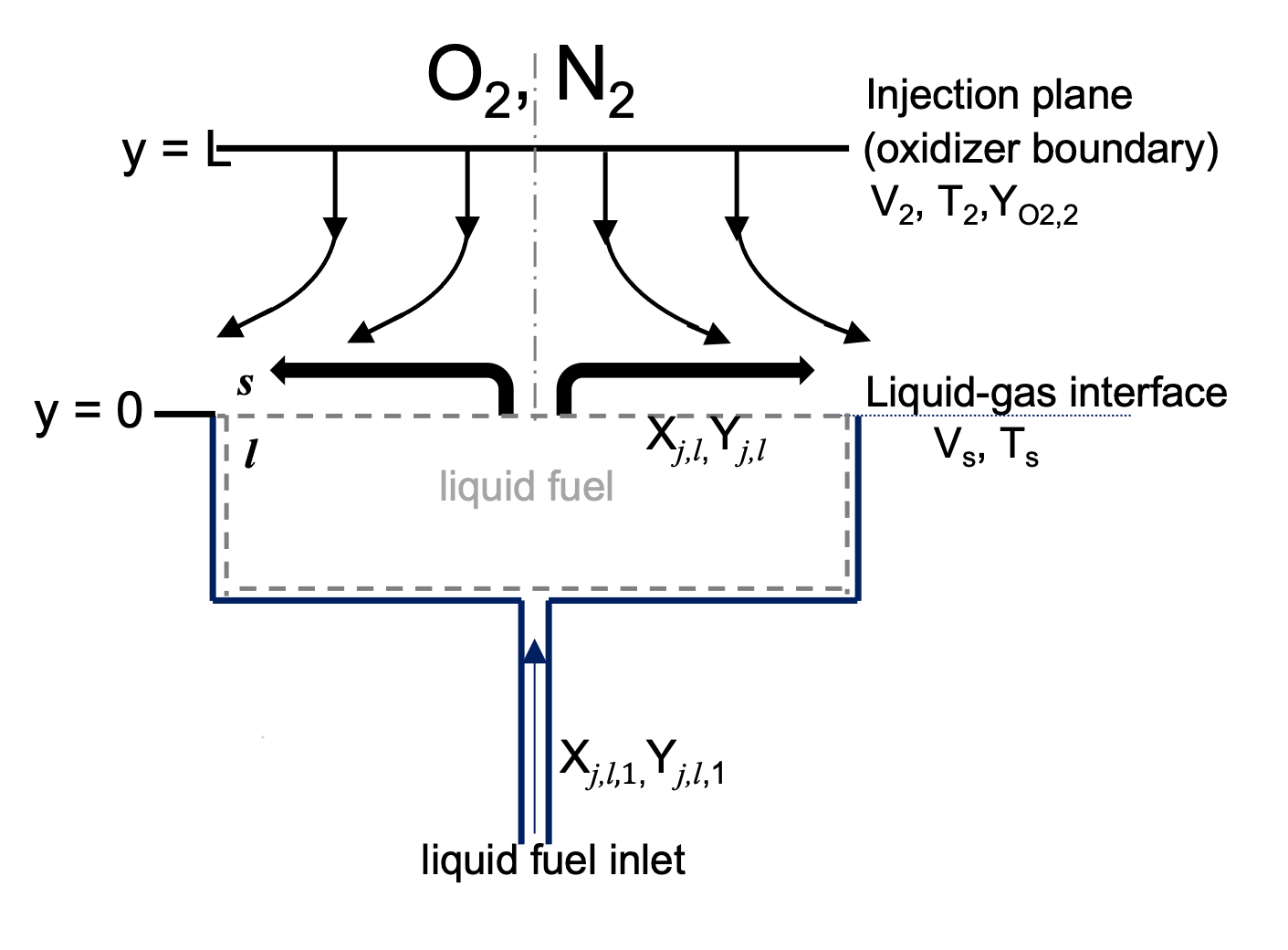
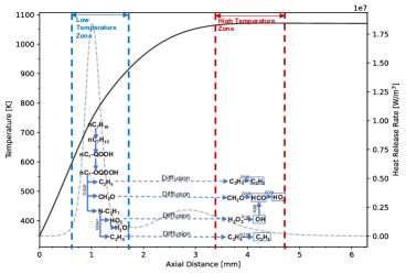
Fig 1 is a schematic illustration of the liquid fuel counterflow configuration used in this computation study. In this configuration, an axisymmetric flow of an oxidizer stream consisting of oxygen and nitrogen is directed over the surface of an evaporating pool of a liquid fuel in a fuel-cup. This flow is injected from the oxidizer boundary, exit of the oxidizer-duct. The origin is placed on the axis of symmetry at the liquid-vapor interface of the liquid pool, and is the axial co-ordinate and the radial co-ordinate and represents the liquid-gas interface. The distance between the liquid-gas interface and the oxidizer boundary is . At the oxidizer boundary , the magnitude of the injection velocity is , the temperature , the density , and the mass fraction of oxygen . Here, subscript represents conditions at the oxidizer boundary. The radial component of the flow velocity at the oxidizer boundary is presumed to be equal to zero. The temperature at the liquid-gas interface is , and the mass averaged velocity on the gas side of the liquid-gas interface is . Here, subscripts and , respectively, represent conditions on the gas-side and the liquid-side of the liquid-gas interface. The quantities and are, respectively, the mole-fraction and mass-fraction of the component in the top surface of liquid pool, and and are, respectively, the mole-fraction and mass-fraction of the component in the liquid that is entering the fuel-cup of the counterflow burner. It has been shown previously [15] that the radial component of the flow velocity at the liquid-gas interface is small and can be presumed to be equal to zero. It has been shown that in the asymptotic limit of large Reynolds number the stagnation plane formed between the oxidizer stream and the fuel vapors is close to the liquid-gas interface and a thin boundary layer is established there. The inviscid flow outside the boundary layer is rotational. The local strain rate, , at the stagnation plane, is given by [16, 15].
2.2 Numerical Simulations
The computations are performed using Cantera [17] C++ interface with modified boundary conditions for liquid-gas interface of the liquid-pool. The mix-average transport model is applied to obtained steady-state solutions. At the oxidizer boundary, the injection velocity , the temperature, , and the value of are specified. At the fuel side, Eq (1) shows the boundary conditions for species conservation and energy conservation that are applied at the liquid-gas interface.
| (1) |
and the constraint . Here subscripts and , respectively, refer to non-evaporating and evaporating species (specifically components of the liquid fuel), is the mass evaporation rate, , and the mass fraction and diffusive flux of the non-evaporating species, , and the mass fraction, mole fraction and diffusive flux of the evaporating species on the gas side of the interface, is the thermal conductivity of the gas, and , and , respectively, are the heat of vaporization and vapor pressure of component on the liquid-side of liquid-gas interface and the total pressure. The total mass flux of all species, , on the gas-side of the liquid-gas interface comprises the diffusive flux, , and the convective flux . The first expression in Eq (1) imposes the condition that the total mass flux for all species, except for those of the evaporating fuel components, vanishes at the liquid-gas interface. The second expression of Eq (1) imposes the constraint that the outgoing mass flux of each evaporating component in the liquid from the liquid-gas interface must be equal to the incoming mass flux, specifically the product of and the mass fraction of the species at liquid pool inlet, . The third expression in Eq (1) is energy balance at the liquid-gas interface, and the fourth expression is Raoult’s law relating the mole-fraction of the evaporating species on the gas side to the corresponding mole-fraction in the liquid. It is noticed that the at the liquid-gas interface is different from liquid pool inlet , considering the properties’ difference among components in the liquid pool
Kinetic modeling is carried out using the San Diego Mechanism [18]. The computer program Cantera is used to compute the flame structure and critical conditions of auto-ignition. Empirical coefficients for calculating the vapor pressure, and the heat of vaporization, for these fuels are from [19].
The simulation procedure for determining the critical conditions of auto-ignition is outlined as follows. The process begins with the establishment of the flow field where volumetric flow rate derived from predefined strain rate for the oxidizer stream. The inlet condition of liquid pool are set and interface boundary of liquid pool boundary will be solved simultaneously. It is crucial to ensure no flame presence detected within the reactive field. The temperature of the oxidizer stream is gradually increased in small increments to obtain steady-state solution until auto-ignition takes place. The temperature of the oxidizer stream at point of auto-ignition, is recorded alongside the predefined strain rate . This simulation is repeated for various mixtures, maintaining same strain rate, to ensure subsequent comprehensive analysis and comparison.
3 Methodology
3.1 Analysis of reaction rate change
Reaction-rate-change-analysis is designed to identify factors, either rate constant or species concentration, that primarily produce variations of rate of the reaction under different conditions. Similar to the approach taken in sensitivity analysis, the calculation of partial derivatives of the reaction rate with respect to the rate constant and species concentration serves as an important tool in this method of analysis.
The rates of forward reaction and reverse reaction are determined by the product of the concentration of reactants or products and their respective rate constants , expressed as follows:
|
|
(2) |
The parameters , represent the stoichiometric coefficients for species appearing as a reactant and as a product, respectively.
In this research, we distinguish between forward and reverse elemental reactions, treating each as distinct entities. It is encapsulated by equation:
|
|
(3) |
Here, m denotes the total number of elementary reactions before their separation into forward and reverse components, while n represents the total number of reactions after separation.
Change of reaction rate distributed to the reaction rate constant change and species concentration change are given as follows:
|
|
(4) |
|
|
(5) |
where the derivatives , and are given by:
|
|
(6) |
|
|
(7) |
with
Here, represents the total number of species involved in the reaction. The term is an approximation of , derived from the Taylor expansion truncated at the first-order derivative. For an augmentation in precision, particularly concerning the reaction rate, , which manifests as a multivariate function, employing the second-order Taylor expansion provides deeper understanding. The formula below outlines the approximated reaction rate from the second-order Taylor expansion for function of multiple variables:
|
|
(8) |
For simplification, let the variable encompasses both the rate constant, , and the species concentration, , with specifically denoting . By employing the second derivative in Taylor series, the change in reaction rate attributed to could be written as:
|
|
(9) |
The term delineates the direct contribution of to , encapsulating both linear and quadratic influences. While, the term quantifies the synergistic influence on emanating from interaction between and . This synergistic influence could be symmetrically attributed to the influence from both and .
3.2 Analysis of heat release rate change
Heat-release-rate-analysis aims to quantify the impact of changes in each species on overall heat release rate under different conditions. Heat release rate, denoted by , is determined by summing the production of reaction enthalpy and net reaction rate for all relevant reactions. The relationship is mathematically represented as:
|
|
(10) |
where signifies the enthalpy change of the reaction and represents the net rate of the reaction. The net reaction rate further delineated as the difference between forward and backward reaction rates:
|
|
(11) |
The expression of heat release rate can be reformulated as follows:
| (12) |
Heat-release-rate-analysis presented in this study primarily focuses on high-temperature zone where oxidizer temperature maintained constantly. Therefore, the local temperature at selected points for various mixtures are nearly identical, allowing for the reasonable assumption that reaction enthalpy , which dependent on local temperature, remains constant. Therefore, the distribution of change of heat release rate, , in response to changes in reaction rate constant, and species concentrations , are defined as follows:
|
|
(13) |
|
|
(14) |
The terms represent the change of heat release rate attributed to the change of reaction rate constant and the change of species concentration
3.3 Analysis of species concentration change
Analysis of species concentration change aims to quantifying the impact of reactions on changes of species and elucidate the interrelation among various species, particularly those achieving steady-state. While for species that do not satisfy steady-state approximation, the analysis incorporates the effects of species diffusion and convection. Furthermore, diagrams illustrating species equation terms provides a visual representation that enhances understanding interactions associated with these species.
For the counterflow flame, in steady state solution, governing equation for species B is given by :
|
|
(15) |
Here, denotes the molecular weight of species B. The production rate of species B is represented by , while symbolizes the consumption rate of species B. The production and consumption rate can be expressed as follows:
| (16) |
| (17) |
with defined as
|
|
(18) |
The term
where , are the stoichiometric coefficients for species B appearing as a reactant and as a product in reaction, respectively.
Governing equation of species B, Eq.(15), could be rewritten as :
|
|
(19) |
While, can be expressed as:
|
|
(20) |
where are defined as:
|
|
(21) |
and indicates whether species is species B:
|
|
(22) |
Combining the Eq (19) and Eq (20), the concentration of substance B, can be derived from following expression:
|
|
(23) |
Upon substituting Eq (16) into the equation above, we could obtain a detailed expression for as:
|
|
(24) |
Here, the terms and correspond to convective and diffusive mass transfer related term of species B, respectively.
With the framework established by Eq (24), we can delve into analyzing changes in the concentration of species B. For the elemental reaction, the contribution of its forward reaction rate with respect to species is delineated as follows:
|
|
(25) |
Similarly, its backward reaction rate contribution with respect to is expressed as:
|
|
(26) |
The contributions of convective mass transfer with respect to changes in are identified as:
|
|
(27) |
Similarly, the contributions of diffusion mass transfer with respect to changes in is expressed as:
|
|
(28) |
Here, sum defined as the aggregate of all contributions to changes in , encapsulating those from both the forward and backward reaction rates, as well as from the convective and diffusive mass transfers:
| sum | ||||
| (29) |
Under the assumption that species B adheres to the steady-state approximation in the counterflow flame, governing equation terms exhibit the following relationship:
|
|
(30) |
This suggests the magnitude of the convective and diffusive terms is considerably less than that of the production and consumption rates of species B. Consequently, upon disregarding the diffusion and convection terms, the concentration of species B, as depicted in Eq (24), simplifies to:
|
|
(31) |
In this approximation, the contributions of both convection () and diffusion () are considered negligible. Furthermore, the term sum simplifies in the steady-state(ss) approximation as follows:
| (32) |
In scenarios where steady-state approximation is not applicable to species , it becomes critical to consider all terms in governing equation, including those related to diffusion and convection. This comprehensive approach acknowledges the comparable significance of diffusion and convection related terms alongside the chemical reaction term:
|
|
(33) |
For the species not in steady state, visualizations delineating equation terms including convection, diffusion and net production terms, across the reactive field could help identify the origin of species undergoing diffusion or convection to other regions.
At a specific location, the dominance of one term over others in species equation highlights its pivotal role in shaping concentration profile. A positive value indicates an enhancement in concentration, whereas a negative value signifies a diminishing effect on concentration profile. This approach is elaborated in results and discussion section.
4 Results and Discussion
The fuels tested in this study include n-heptane, ethanol, and their mixtures with volumetric composition of 20% n-heptane + 80% ethanol, 30% n-heptane + 70% ethanol, 50% n-heptane + 50% ethanol, 80% n-heptane + 20% ethanol, and 90% n-heptane + 10% ethanol. The oxidizer used is air.
4.1 Auto-ignition temperature and heat release rate analysis
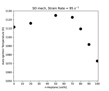
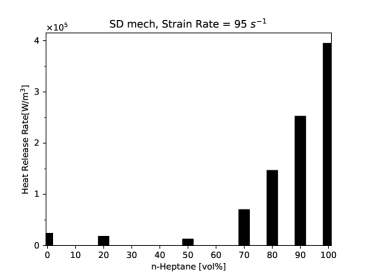
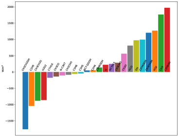
Fig. 2 illustrates auto-ignition temperature calculated at low strain rate, 95 for various volume fraction of ethanol in n-heptane. Additionally, Fig. 3 illustrates the variations in heat release rate, prior to auto-ignition, for these mixtures within the high-temperature zone, particularly focusing at 4.3mm from the fuel stream inlet, which corresponds to an oxidizer temperature, T, of 1060K. A comparison between Fig. 2 and Fig. 3 indicates a direct correlation between the magnitude of heat release rate in this zone and the requisite temperature of auto-ignition (Tig). Among these examined mixtures, the 50%n-heptane-50%ethanol blend stands out, necessitating the highest Tig, a phenomenon that can be attributed to its significant lowest peak in heat release rate.
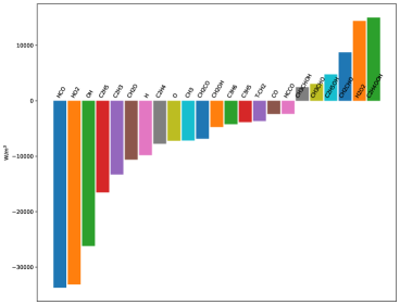
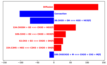
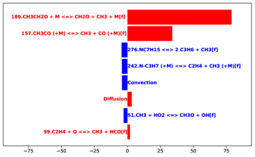
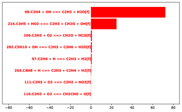
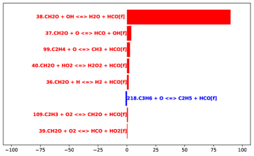
Fig. 3 illustrates that reducing the volume fraction of heptane from 100% to 90% leads to a significant decrease in heat release rate. Further heat-release-rate-analysis, as depicted in Fig. 4, attributes this decline of heat release rate predominantly and directly to changes of concentrations of \ceHCO, \ceHO2, \ceOH, \ceC2H5, \ceC2H3, \ceCH2O.
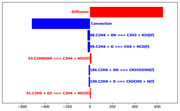
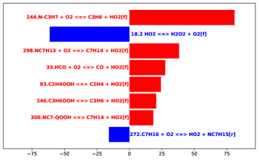
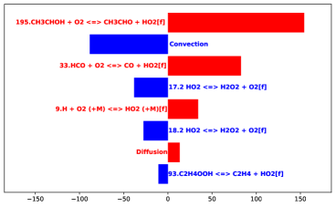
In contrast, the reduction in volume fraction of n-heptane from 50% to 20% is correlated to observable increase in heat release rate, as illustrated in Fig. 3. Similar heat-release-rate-analysis conducted and shown in Fig. 5, which indicated the increase of heat release rate is attributed to involvement of species such as \ceCH3, \ceHO2, \ceOH, \ceHCO, \ceC2H5OH, \ceCH3CHOH, \ceCH2O.
4.2 key species in n-heptane-dominant mixtures
The species contributing to heat release rate change could be categorized into two groups based on satisfaction of the steady-state approximation at the selected location.
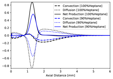
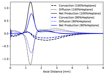
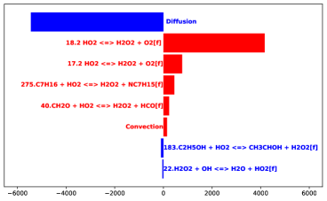
For species that not satisfied steady-state approximation, their concentrations are governed by a combination of the diffusion term, convection term and chemical reaction term in species equation. Specifically, in Fig. 6, for \ceCH2O , the net production rate peak is observed around 1.2mm, located in low-temperature zone where the LTC is highly activated. Additionally, positive value of diffusion term between 2mm and 5mm elucidate the role of diffusion term in promoting the transport of the \ceCH2O from the low-temperature zone to the high-temperature zone. Consequently, a decline of activity of LTC in the low-temperature region, caused by additional ethanol, leads to a reduction of diffusion effect, subsequently impacting heat release rate and auto-ignition at the high-temperature region. This effect is also evidenced by analysis of \ceCH2O concentration change, depicted in Fig. 7. The observed reduction of \ceCH2O in the high-temperature region is primarily attributed to decrement in diffusion term.
Similar patterns are observed with other radicals, such as hydroperoxyl (\ceH2O2), ethylene (\ceC3H6), and formaldehyde (\ceC2H4). The corresponding analyses and plots for these species are included in the supplemental materials, ranging from Fig. 21 to Fig. 24.
Within the context of steady-state species, their concentrations are predominantly governed by the the equilibrium between production and consumption rates at selected location. Among the species implicated in heat release rate reduction, \ceHCO, \ceHO2, \ceOH, \ceC2H5 and \ceC2H3 are identified to be in the steady-state, indicating they produced at selected location concurrently consumed. The fluctuations in their concentrations were affected by specific reactions and variation of other species, elucidated through the analysis of concentration change.
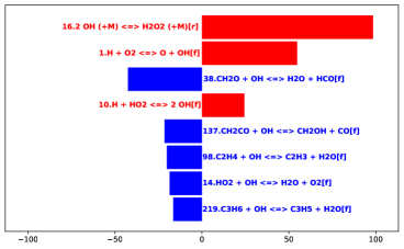
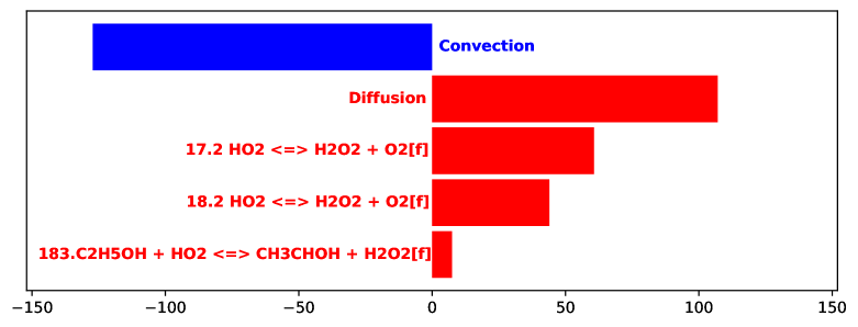
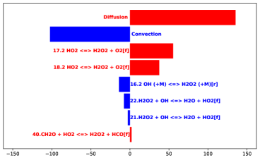
Fig. 8 demonstrates that concentration change of radical \ceOH at the high-temperature zone primarily affected by reverse reaction of R16:2 \ceOH (+M) \ceH2O2 (+M) , involving the decomposition of \ceH2O2. \ceH2O2 is not in steady state and is diffused from the low-temperature zone.
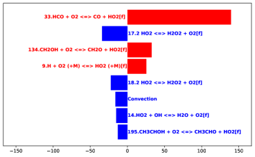
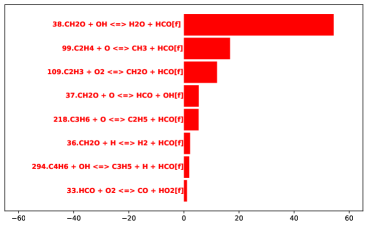
Further concentration analysis reveals that concentration of \ceHO2 is predominantly controlled by \ceHCO, through R33: \ceHCO + \ceO2 \ceCO + \ceHO2. Similarly, \ceHCO concentration are primarily controlled by \ceCH2O and \ceOH via R38: \ceCH2O + \ceOH H2O + \ceHCO. Concentration of \ceC2H3 is primarily regulated by \ceC2H4 by R98: \ceC2H4 + \ceOH \ceC2H3 + H2O. Illustrative plots of these relationships are provided in the supplemental materials, as seen in Figures 25, 26, and 27. As mentioned before, both \ceCH2O and \ceC2H4 are mainly transported from the low-temperature region via diffusion.
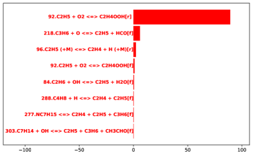
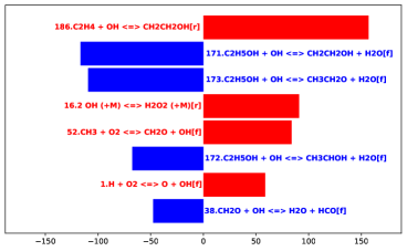
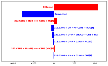
Fig. 9 reveals that the radical \ceC2H5 is primarily influenced by R92: \ceC2H5+\ceO2=\ceC2H4OOH. However, it is actually a fast reaction so that the substantial consumption of \ceC2H5 in the forward reaction is counterbalanced by its production in the reverse reaction. Therefore, greater emphasis should be placed to the second reaction depicted in Fig. 9, R218: \ceC3H6 + O \ceC3H6 + \ceHCO, which is primarily affected by \ceC3H6. Notably, \ceC3H6 is not in the steady state at the high-temperature zone and is primarily diffused from the low-temperature region.
In summary, radicals including \ceCH2O, \ceC2H4, \ceC3H6 and \ceH2O2 predominantly diffused from the low-temperature zone, significantly influencing the heat release rate and auto-ignition process in the high-temperature zone.
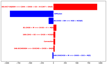
This observation underscores the necessity of delineating the production mechanism of these species in the low-temperature zone. As indicated in Fig. 10 and Fig. 11, \ceCH2O and \ceC2H4 primarily produced through reaction R302: NC7OQOOH \ceC2H4 + \ceCH2O + \ceCO + \ceNC3H7 + \ceOH at the low-temperature zone.
The origins of \ceC3H6 and \ceH2O2 in the low-temperature zone is notably complex. Fig. 12 proves that concentration of \ceC3H6 is predominantly regulated by \ceNC3H7. Similarly, concentration analysis of \ceH2O2 and \ceHO2 indicate \ceH2O2 is mainly converted from \ceHO2, which, in turn, is affected by \ceNC3H7. . These analysis results are further detailed in the supplemental materials, specifically in Figures 28 and 29.
Given its pivotal role, \ceNC3H7 emerges as a crucial species impacting both \ceH2O2 and \ceC3H6. It is primarily produced through reaction R302, as indicated in Fig. 13. Thus, in the low-temperature region, R302 exerts a direct influence on producing \ceCH2O, \ceC2H4, while indirectly affecting \ceC3H6 and \ceHO2 via \ceNC3H7.
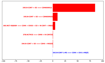
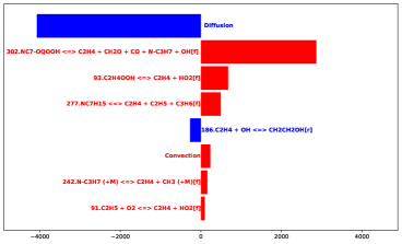
Fig. 14 provides a comprehensive overview elucidating interplay between the low and high temperature zones in n-heptane-dominant mixtures. The addition of ethanol leads to competition of oxygen, resulting in a decreased of \ceNC7OQOOH concentration in the low-temperature zone. This reduction in concentration of \ceNC7OQOOH subsequently diminishes the reaction rate of R302 and concentrations of its products. Ultimately, these effects propagated to the high-temperature zone through species diffusion.
4.3 key species in ethanol-dominant mixtures
With the decrease of n-heptane’s volume fraction from 50% to 20% and a concurrent increase in ethanol’s volume fraction from 50% to 80%, it is observed the elevation in heat release rate in the high-temperature zone. This is primarily due to ethanol undergoing decomposition into three major products through hydrogen abstraction: \ceCH3CHOH, \ceCH2CH2OH and \ceCH3CH2O.
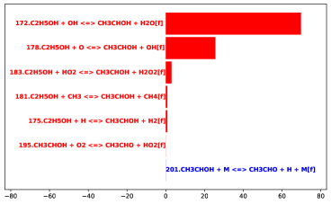
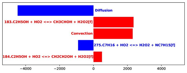
The production of \ceCH3CHOH, mainly from reactions R172: \ceC2H5OH + \ceOH \ceCH3CHOH + H2O and R178: \ceC2H5OH + O \ceCH3CHOH + \ceOH, plays a significant role in increasing heat release rate, as confirmed in Fig. 15. Notably, one pathway to form \ceCH3CHOH, via R183: \ceC2H5OH + \ceH2O2 \ceCH3CHOH + \ceH2O2, is accompanied by a significant production of \ceH2O2, as depicted in Fig. 16(b), with the peak production around 2.0mm-2.2mm, shown in Fig. 16(a). It is subsequently diffused to the high-temperature region, contributing to the increase of \ceOH concentration through the reverse reaction of R16: \ceH2O2 (+M) 2 \ceOH (+M), corroborated by Fig. 17. Additionally, the reverse reaction of R186, involving the decomposition of \ceCH2CH2OH, contributes to the elevation of \ceOH concentration, as indicated in Fig. 17.
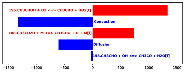
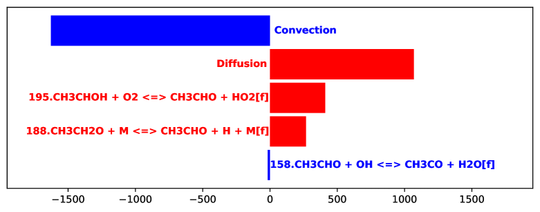
Furthermore, Fig. 18(a) demonstrates that the elevated levels of \ceCH3CHOH (through R195) and \ceCH3CH2O (through R188) lead to an increase in \ceCH3CHO. And Fig. 18(b) further confirmed that part of increasing \ceCH3CHO diffused to the high-temperature region, thereby promoting heat release rate.
As illustrated in Fig. 19, the decomposition of \ceCH3CH2O into \ceCH3 and \ceCH2O through R189 : \ceCH3CH2O (+M) \ceCH3 + \ceCH2O (+M), with these products subsequently diffused to the high-temperature region. This process is augmented by R52: \ceCH3 + \ceO2 \ceCH2O + \ceOH, as illustrated in , wherein \ceCH3 reacts with \ceO2, further elevating the concentration of \ceCH2O. The increase in \ceCH2O and \ceOH leads to a rise in \ceHCO, increasing \ceHCO contributes to enhanced concentration of \ceHO2 in the high-temperature region. The concentration change analysis related to \ceCH2O, \ceHCO and \ceHO2 are provided in Fig. 30, Fig. 31 and Fig. 32 in supplemental materials.
The reaction pathway including \ceCH2O, \ceHCO and \ceHO2 exhibits similarity in both n-heptane-dominant and ethanol-dominant mixtures. However, the concentration of \ceCH2O in n-heptane-dominant mixtures is predominantly influenced by the low-temperature chemistry of n-heptane, whereas in ethanol-dominant mixtures, \ceCH2O is significantly affected, directly and indirectly, by \ceCH3CH2O, through ethanol’s hydrogen abstraction reaction, R189.
Additionally, the increase in \ceHO2 partially results in heightened level of \ceH2O2 at the high-temperature region, as evidenced in Fig. 16(b).
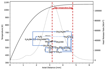
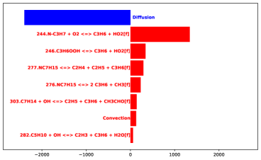
Fig. 20 succinctly summarizes the reaction pathways and diffusive effects associated with ethanol-dominant mixtures. The observed increase in heat release rate, as ethanol volume fraction increased from 50% to 80%, is primarily attributable to species and reactions associated with ethanol’s chemistry. In these mixtures, the influence of the inhibition of LTC is considered negligible.
5 Conclusion
This work delves into the relationship between change in heat release rate and variations in species, elucidating interaction among related species and the potential influence of species transport across temperature zones. This investigation specifically targets n-heptane and ethanol dominant mixtures under the counterflow flame configuration. By employing the sensitivity method introduced earlier, it provides a detailed explanation of variation of auto-ignition temperatures at low strain rate.
Simulation result indicates the correlation between heat release rate and auto-ignition temperature. Further quantitative analyses, utilizing the proposed method, reveals heat release rate change in both n-heptane and ethanol dominant mixtures are directly associated with alteration of several key species within the high-temperature zone.
In n-heptane-dominant mixtures, the investigation reveals that steady-state species at the high-temperature zone, including hydroxyl radicals (\ceOH) and hydroperoxyl radicals (\ceHO2), are in maintaining the equilibrium between production and consumption rate, directly affecting heat release rate. Non-steady-state species at the high-temperature zone, such as \ceCH2O and \ceC2H4 play significant roles in the auto-ignition process, primarily due to their involvement in LTC at the low-temperature zone and subsequent diffusion to the high-temperature region.
For ethanol-dominant mixtures, the study highlights the observed increase in heat release rate with the increase in ethanol’s volume fraction, attributing this elevation to the decomposition of ethanol into major products including \ceCH3CHOH, \ceCH2CH2OH and \ceCH3CH2O radicals. The production of these species, particularly through hydrogen abstraction reactions is identified as the key pathway driving the observed increase in heat release rate.
The analysis result emphasizes the important role of species diffusion in the the interaction between low and high temperature zones in n-heptane-dominant mixtures. Additionally, in the ethanol dominant mixtures, chemical kinetics are notably unaffected by n-heptane’s LTC, highlighting the distinctive chemical pathways of ethanol and the influence of fuel composition on auto-ignition and heat release rate.
In summary, this study provides valuable insights into interplay between n-heptane and ethanol dominant mixtures in the counterflow diffusion flame, offering a detailed understanding of the roles of key chemical species and their interactions across different temperature zones. The findings underscore the importance of considering both the chemical kinetics and species diffusion effect in 1D flame modeling to predict the combustion behavior of complex fuel mixtures. Future research directions may include applying the method of analysis under varying strain rates. Given the complexity of preparing the overview for various mixtures, future efforts should focus on streamlining the analysis process through enhancing code automation.
Supplementary material
Appendix A Concentration Analysis Results
A.1 n-Heptane Dominant Mixtures
A.2 Ethanol Dominant Mixtures
References
- [1] S. Liu, J. C. Hewson, J. H. Chen, H. Pitsch, Effects of strain rate on high-pressure nonpremixed n-heptane autoignition in counterflow, Combustion and Flame 137 (3) (2004) 320–339. doi:https://doi.org/10.1016/j.combustflame.2004.01.011.
- [2] R. Seiser, H. Pitsch, K. Seshadri, W. Pitz, H. Gurran, Extinction and autoignition of n-heptane in counterflow configuration, Proceedings of the Combustion Institute 28 (2) (2000) 2029–2037. doi:https://doi.org/10.1016/S0082-0784(00)80610-4.
- [3] J. Herzler, L. Jerig, P. Roth, Shock tube study of the ignition of lean n-heptane/air mixtures at intermediate temperatures and high pressures, Proceedings of the Combustion Institute 30 (1) (2005) 1147–1153. doi:https://doi.org/10.1016/j.proci.2004.07.008.
- [4] C. Xie, M. Lailliau, G. Issayev, Q. Xu, W. Chen, P. Dagaut, A. Farooq, S. M. Sarathy, L. Wei, Z. Wang, Revisiting low temperature oxidation chemistry of n-heptane, Combustion and Flame 242 (2022) 112177. doi:https://doi.org/10.1016/j.combustflame.2022.112177.
- [5] T. I. Farouk, F. L. Dryer, Isolated n-heptane droplet combustion in microgravity: “cool flames” – two-stage combustion, Combustion and Flame 161 (2) (2014) 565–581. doi:https://doi.org/10.1016/j.combustflame.2013.09.011.
- [6] J. Zhang, S. Niu, Y. Zhang, C. Tang, X. Jiang, E. Hu, Z. Huang, Experimental and modeling study of the auto-ignition of n-heptane/n-butanol mixtures, Combustion and Flame 160 (1) (2013) 31–39. doi:https://doi.org/10.1016/j.combustflame.2012.09.006.
- [7] S. Guo, A. Cuoci, Y. Wang, C. T. Avedisian, L. Ji, K. Seshadri, N. DiReda, F. Alessio, Combustion characteristics of a tier ii gasoline certification fuel and its surrogate with iso-butanol: experiments and detailed numerical modeling, Tech. rep., American Chemical Society, Chicago, Ill. (2022).
- [8] Z. Yang, Y. Qian, X. Yang, Y. Wang, Y. Wang, Z. Huang, X. Lu, Autoignition of n-butanol/n-heptane blend fuels in a rapid compression machine under low-to-medium temperature ranges, Energy & Fuels 27 (12) (2013) 7800–7808. doi:10.1021/ef401774f.
- [9] P. Saisirirat, F. Foucher, S. Chanchaona, C. Mounaïm-Rousselle, Spectroscopic measurements of low-temperature heat release for homogeneous combustion compression ignition (hcci) n-heptane/alcohol mixture combustion, Energy & Fuels 24 (10) (2010) 5404–5409. doi:10.1021/ef100938u.
- [10] L. Ji, A. Cuoci, A. Frassoldati, M. Mehl, T. Avedisian, K. Seshadri, Experimental and computational investigation of the influence of iso-butanol on autoignition of n-decane and n-heptane in non-premixed flows, Proceedings of the Combustion Institute 39 (2) (2023) 2007–2015. doi:https://doi.org/10.1016/j.proci.2022.08.058.
-
[11]
H. Rabitz, M. Kramer, D. Dacol,
Sensitivity analysis
in chemical kinetics, Annual Review of Physical Chemistry 34 (1) (1983)
419–461.
URL https://api.semanticscholar.org/CorpusID:97123635 - [12] T. Turanyi, Applications of sensitivity analysis to combustion chemistry, Reliability Engineering and System Safety 57 (1) (1997) 41–48, the Role of Sensitivity Analysis in the Corroboration of Models and its Links to Model Structural and Parametric Uncertainty. doi:https://doi.org/10.1016/S0951-8320(97)00016-1.
- [13] T. A. O. Kalen Braman, V. Raman, Adjoint-based sensitivity analysis of flames, Combustion Theory and Modelling 19 (1) (2015) 29–56. doi:10.1080/13647830.2014.976274.
- [14] J. M. Zurada, A. Malinowski, S. Usui, Perturbation method for deleting redundant inputs of perceptron networks, Neurocomputing 14 (2) (1997) 177–193. doi:https://doi.org/10.1016/S0925-2312(96)00031-8.
- [15] K. Seshadri, S. Humer, R. Seiser, Activation-energy asymptotic theory of autoignition of condensed hydrocarbon fuels in non-premixed flows with comparison to experiment, Combustion Theory and Modelling 12 (2008) 831–855. doi:10.1080/13647830802054207.
- [16] K. Seshadri, F. A. Williams, Laminar flow between parallel plates with injection of a reactant at high reynolds number, International Journal of Heat and Mass Transfer 21 (2) (1978) 251–253. doi:https://doi.org/10.1016/0017-9310(78)90230-2.
- [17] D. G. Goodwin, Moffat, H. K, S. Ingmar, Speth, R. L, Weber, B. W., Cantera: An object-oriented software toolkit for chemical kinetics, thermodynamics, and transport processes., version 3.0.0 (2023). doi:10.5281/zenodo.8137090.
- [18] The San Diego Mechanism, http://web.eng.ucsd.edu/mae/groups/combustion/mechanism.html (2016).
- [19] C. L. Yaws, Yaws’ Handbook of Thermodynamic and Physical Properties of Chemical Compounds, Knovel, 2003.