Beyond Boolean networks, a multi-valued approach

Abstract.

Boolean networks can be viewed as functions on the set of binary strings of a given length, described via logical rules. They were introduced as dynamic models into biology, in particular as logical models of intracellular regulatory networks involving genes, proteins, and metabolites. Since genes can have several modes of action, depending on their expression levels, binary variables are often not sufficiently rich, requiring the use of multi-valued networks instead. The steady state analysis of Boolean networks is computationally complex, and increasing the number of variable values beyond $2$ adds substantially to this complexity, and no general methods are available beyond simulation. The main contribution of this paper is to give an algorithm to compute the steady states of a multi-valued network that has a complexity that, in many cases, is essentially the same as that for the case of binary values. Our approach is based on a representation of multi-valued networks using multi-valued logic functions, providing a biologically intuitive representation of the network. Furthermore, it uses tools to compute lattice points in rational polytopes, tapping a rich area of algebraic combinatorics as a source for combinatorial algorithms for Boolean network analysis. An implementation of the algorithm is provided.

1. Introduction

Boolean networks have been used in computer science, engineering, and physics extensively. They were introduced into biology by Stuart Kauffman [Kauffman69], as a model class for intracellular regulatory networks, viewed as logical switching networks rather than as biochemical reaction networks. This has proven very useful, in part because their specification is intuitive from a biological point of view, and there are now hundreds of published Boolean network models of this type. A major drawback of this model type is the absence of mathematical tools for their analysis, in particular the efficient computation of steady states. For models with a small number of variables, exhaustive model simulation is feasible, while for larger models, a common method is sampling of the state space of the model.

For applications of this modeling framework to biology, it is often useful to be able to assume that certain variables have more than two possible values. For gene regulation, for instance, a given gene may have several models of action, depending on its expression levels (several examples are given below). In order to capture this complexity, a variable might need to take on several different values, such as “0 (off), 1 (medium expression), 2 (high expression).” The functions governing such networks can be expressed in terms of multi-valued logic, and we refer to them as multi-valued networks. The steady state analysis becomes significantly more complex.

This paper presents an algorithm to carry out such an analysis in a computationally high efficient way. We first make the problem more precise. Given $n$ interacting (biological) species whose values can be described by $m+1$ values, we can establish a bijection between the set of values and the set

(1) $$X_{m}=\big{\{}0,\frac{1}{m},\frac{2}{m},\dots,\frac{m-1}{m},1\big{\}}.$$

In particular, if $m=1$, we have a Boolean network. Our aim is to study the dynamics of the iteration of a function $f:X_{m}^{n}\to X_{m}^{n}$, with synchronous variable update. (Note that the order in which individual variables are updated, whether synchronous or asynchronous, does not change the steady states of the system.)

Any function on $n$ variables defined over a finite set $X$ of cardinality a power of a prime number can be thought as a function over a finite field. Moreover, it can be expressed as a polynomial function with coefficients in this field, and this opens the use of tools from computational algebraic geometry as Gröbner bases [VCJL]. The advantage is that it is not necessary to express the function via a whole (big) table. For instance, given a function $f:X^{n}\to X^{n}$, we can find the fixed points $\{x\in X^{n}\,:\,f(x)=x\}$ of $f$ (also known as steady states) solving the square polynomial system $f(x)-x=0$. In [BFSS13] the authors show that in the Boolean case $m=1$, it is possible to compute the fixed points with complexity $O(2^{0.841n})$ (under some hypotheses), while the bound for exhaustive search is $4\,{\rm log}_{2}(n)\,2^{n}$.

In [LC10] the authors study multilinear functions representing network functions $f:X_{m}^{n}\to X_{m}$ on a multivalued network. We propose instead to use in the multivariate setting the operations $\odot$, $\oplus$ and $\mathrm{neg}$ introduced in Section 2 that come from multivalued logic [Cignoli, Epstein]. These operations are more intuitive and closer to biological interpretations than the usual operations of polynomials over a finite field (and there is no restriction on the number of values). See for instance Figure 1, that features an example of two interacting nodes, with three values each, where the second variable acts as a repressor of the first one. The update function of the first node, $f_{1}$, is represented both as a polynomial over the field with $3$ elements, which gives no clue of its behaviour, and in terms of the logic operations, whose interpretation is transparent.

$\begin{array}[]{c||c|c|c}x_{1}\setminus x_{2}&0&1&2\\ \hline\cr\hline\cr 0&0&0&0\\ \hline\cr 1&1&0&0\\ \hline\cr 2&2&1&0\\ \end{array}$

(a) $f_{1}:\mathbb{F}_{3}^{2}\to\mathbb{F}_{3}$ $f_{1}(x_{1},x_{2})=x_{1}+2x_{1}x_{2}+x_{1}^{2}x_{2}+x_{1}x_{2}^{2}+x_{1}^{2}x_{2}^{2}$

$\begin{array}[]{c||c|c|c}x_{1}\setminus x_{2}&0&\frac{1}{2}&1\\ \hline\cr\hline\cr 0&0&0&0\\ \hline\cr\frac{1}{2}&\frac{1}{2}&0&0\\ \hline\cr 1&1&\frac{1}{2}&0\\ \end{array}$

(b) $f_{1}:\{0,1/2,1\}^{2}\to\{0,1/2,1\}$ $f_{1}(x_{1},x_{2})=x_{1}\circleddash x_{2}$.

Figure 1. (a) The nodes take the values $\{0,1,2\}$ and the polynomial $f_{1}\in\mathbb{F}_{3}[x_{1},x_{2}]$ summarizes the values in the table. (b) The nodes take the values $\{0,1/2,1\}$ and the table is the translation of the first one; the function $f_{1}=x_{1}\circleddash x_{2}$ accounts for the repression shown in the table.

Why model the qualitative behaviour of biological networks with more than two values? The setting of Boolean networks owes much to the work of the Belgian scientist René Thomas. His research included DNA biochemistry, genetics, biophysics, mathematical biology, and dynamical systems. His purpose was to decipher the key logical principles at the basis of the behaviour of biological systems and how complex dynamical behaviour could emerge. He realized that the researcher’s intuition was not enough to understand the intrincated biological regulatory networks and he then proposed to formalize the models using the operations in Boolean algebra, where variables take only two values ($0$ or OFF and $1$ or ON) and the logical operators are AND, OR and NOT, starting with [Thomas73]. In [Thomas91] he argues that even if one is interested in a logical description, the binary case could be too simple in many cases of interest. He adds that for instance, when there is a variable with more than a single action, different levels might be required to produce different effects. However, there are still few articles dealing with multivalued models.

Even if we work with a synchronous update of the nodes, we present in Example 25 a small network extracted from the foundational book [Thomas_DAri], where the synchronous multivalued setting can model the features of an asynchronous model, as the networks become more expressive. Boolean networks became an effective mathematical tool to model many different phenomena in science and engineering and their development has attracted the interest of too many researchers to be cited here. One interesting feature is to understand well how the dynamics of a Boolean network could have high complexity, even if it is composed of simple elementary units [R23].

We show that via the proposed operations of multivalued logic, which are indeed expressed in terms of linear inequalities, we can recover most of the good properties of Boolean networks. Moreover, we show that the computation of fixed points can be done algorithmically for any $m$ using tools to find lattice points in rational polytopes and that in many cases, the complexity to compute the fixed points is essentially the same as in the Boolean setting. This is an alternative to translating a multivalued model into a partial Boolean one, but with $mn$ nodes (see for instance [Tonello] and the references therein).

In Section 2 we introduce the logic operations $\oplus,\odot,\mathrm{neg}$ together with their main properties and we give, in Theorem 10, a constructive way of turning data from a table into an expression of the function in terms of $\odot,\mathrm{neg}$ and constant functions. When modeling biological networks, it is useful to have in mind the behaviour of different small networks that appear frequently as subnetworks of bigger ones, called motifs. We also show in this section the behavior of several small motifs.

In § 3, we further show how to algorithmically translate any network into a $\odot$-$\mathrm{neg}$ network and we show in Theorem 24 how to recover the fixed points. In § 4 we propose several possible reductions of the number of variables (inspired by [VCLA] in the Boolean setting) without increasing the indegree, that is, without increasing the maximum number of variables on which each variable depends (see Proposition 28). We present in § 4.2 an example which is the translation to our setting of an interesting network extracted from www.cellcolective.org, where the number of nodes eventually decreases. In the most interesting cases, the computation is too heavy to be done by hand and we used our publicly available implementation [Aye] that we explain in the next section.

In § 5, we address the computation of fixed points for $\odot$-$\mathrm{neg}$ networks. As we mentioned, this gives in turn the fixed points of any network function $F:X_{m}^{n}\to X_{m}^{n}$ by Theorem 24. One crucial algorithmic fact for $\odot$-$\mathrm{neg}$ networks is Theorem 29 that allows us to automatize the computations without simulations, which would be too costly in general. We present the basic setting for our implementation in Algorithm 2 and we discuss the cost of these computations. When the hypotheses of Theorem 33 do not hold, one needs to count the number of lattice points in a rational polytope, that is, all the integer solutions of a system of inequalities given by linear forms with integer coefficients defining a bounded region. Barvinok proposed in [Barvinok] an algorithm that counts these lattice points in polynomial time when the dimension of the polytope is fixed. The theoretical basis was given by Brion in the beautiful paper [Brion], where he uses the relation of rational polytopes with the theory of toric varieties and results in equivariant $K$-theory. We exemplify the use of our free app for the computation of fixed points in the network introduced in § 4.2.

In Section 6 we present a multi-valued model for the denitrification network in Pseudomonas aeruginosa based on the time-discrete and multi-valued deterministic model introduced in [ABL]. P. aeruginosa can perform (complete) denitrification, a respiratory process that eventually produces atmospheric N₂. The external parameters in the model and some variables are treated as Boolean (low or high), and other variables are considered ternary (low, medium or high). The update rules are formulated in  [ABL] in terms of MIN, MAX and NOT (which correspond to AND, OR and NOT in a Boolean setting). However, the regulations of a few variables cannot be expressed in terms of these operators (marked with a * in the column “Update Rules” in their Table 3). As stated in Theorem 10, any function can be written in terms of constants and the logical operations $\oplus,\odot,\mathrm{neg}$ we propose to use in this paper, so we exactly represent their Update Rules and find the fixed points using results along the paper. Some details are provided in an Appendix.

2. Our setting

This section introduces the basic operations in multivalued logic and how we use them to represent the functions in biological models.

We fix a natural number $m$ and consider networks with $m+1$ values in the set

(2) $$X_{m}=\big{\{}0,\frac{1}{m},\frac{2}{m},\dots,\frac{m-1}{m},1\big{\}}\subset[0,1].$$

Boolean networks are a particular case when $m=1$. As $X_{m}$ is a subset of $\mathbb{R}$, we can also consider the standard operations of addition/substraction ($+/-$) and multiplication (.) on the real line. However, we introduce in the multivariate setting the operations $\odot$, $\oplus$ that come from multivalued logic [Cignoli, Epstein], which are more intuitive and closer to biological interpretations.

2.1. The MV operations

The three basic operations in multivalued logic that we use to build all the functions that we consider are introduced in the following definition:

Definition 1.

We consider the following operations/maps on $X_{m}$:

(3) $$\mathrm{neg}:X_{m}\rightarrow X_{m},\text{ where }\mathrm{neg}(x)=1-x.$$

(4) $$\oplus:X_{m}\times X_{m}\rightarrow X,\text{ where }x\oplus y=min\{1,x\boldsymbol{+}y\}.$$

(5) $$\odot:X_{m}\times X_{m}\rightarrow X_{m},\text{ where }x\odot y=max\{0,x+y-1\}.$$

Example 2.

When $m=2$, the operations (4) and (5) in chart presentation are as follows:

$$\begin{array}[]{c||c|c|c}\oplus&0&\frac{1}{2}&1\\ \hline\cr\hline\cr 0&0&\frac{1}{2}&1\\ \hline\cr\frac{1}{2}&\frac{1}{2}&1&1\\ \hline\cr 1&1&1&1\\ \end{array}\hskip 28.45274pt\begin{array}[]{c||c|c|c}\odot&0&\frac{1}{2}&1\\ \hline\cr\hline\cr 0&0&0&0\\ \hline\cr\frac{1}{2}&0&0&\frac{1}{2}\\ \hline\cr 1&0&\frac{1}{2}&1\\ \end{array}$$

Remark 3.

The following relations between $\oplus$ and $\odot$, which are formally equal to the De Morgan’s law between AND and OR in the Boolean case, hold:

(6) $$x\odot y=\mathrm{neg}(\mathrm{neg}(x)\oplus\mathrm{neg}(y)),$$

(7) $$x\oplus y=\mathrm{neg}(\mathrm{neg}(x)\odot\mathrm{neg}(y)).$$

We list in the following proposition other useful properties which are straightforward to prove.

Proposition 4.

Given $m$ and $X_{m}$ as in (2), consider the operations defined in Definition 1. The following properties hold:

1. $\mathrm{neg}(0)=1$ and $\mathrm{neg}(1)=0$.

2. The product of several variables can be expressed as

   $$x_{1}\odot\dots\odot x_{n}=\max\{0,x_{1}+\dots+x_{n}-(n-1)\}.$$

3. Analogously,

   $$x_{1}\oplus\dots\oplus x_{n}=\min\{1,x_{1}+\dots+x_{n}\}.$$

4. The product $\odot$ is associative and commutative.

5. $0\odot x=0$ and $1\odot x=x$ for any $x\in X$.

6. For any finite index set $I$, $\mathrm{neg}(\bigoplus_{i\in I}a_{i})=\bigodot_{i\in I}\mathrm{neg}(a_{i})$.

7. $\max\{x,y\}\,=\,(x\odot\mathrm{neg}(y))\oplus y$.

8. $\min\{x,y\}=\,(x\oplus\mathrm{neg}(y))\odot y$.

9. $x\leq y$ if and only if $x\odot\mathrm{neg}(y)=0$.

10. $x\odot y=0$ if and only if $x+y\leq 1$. More in general, $x_{1}\odot\dots\odot x_{n}=0$ if and only if $x_{1}+\dots+x_{n}\leq(n-1)$.

Remark 5.

Associativity will allow us to avoid writing parentheses in some cases. More precisely, we will write $s_{1}(x_{1})\odot s_{2}(x_{2})\odot s_{3}(x_{3})$ instead of $\big{(}s_{1}(x_{1})\odot s_{2}(x_{2})\big{)}\odot s_{3}(x_{3})\hskip 11.38109pt\hbox{or}\hskip 11.38109pts_{1}(x_{1})\odot\big{(}s_{2}(x_{2})\odot s_{3}(x_{3})\big{)}$ for $s_{i}(x_{i})=x_{i}$ or $s_{i}(x_{i})=\mathrm{neg}(x_{i})$.

On the other hand, the operations we defined do not satisfy distributivity. In general, $(x\oplus y)\odot z\neq(x\odot z)\oplus(y\odot z)$. Consider for example $m=5,x=\frac{3}{5},y=\frac{2}{5},z=\frac{1}{5}$ then $(x\oplus y)\odot z=\frac{1}{5}$ while $(x\odot z)\oplus(y\odot z)=0.$

Definition 6.

We also define the substraction, exponentiation and multiplication by a positive integer $k\in\mathbb{N}$ as:

(10) $$x\circleddash y :=x\odot\mathrm{neg}(y)=\max\{0,x-y\}=\left\{\begin{array}[]{lcc}x-y&if&x-y\geq 0\\ 0&otherwise&\end{array}\right.,$$

(11) $$x^{k} :=\underset{k\text{ times}}{\underbrace{x\odot\dots\odot x}}=\max\{0,kx-(k-1)\},$$

(12) $$kx :=\underset{k\text{ times}}{\underbrace{x\oplus\dots\oplus x}}=\min\{1,kx\}.$$

Remark 7.

Note that $x\odot y\leq x$ for any $x,y\in X_{m}$, and equality holds only when $y=1$ or $x=0$. In particular, $x^{k}\leq x$ for any $x\in X_{m}$ and any $k\in\mathbb{N}$, with equality only when $x=0,1$ or $k=1$.

Remark 8.

It is interesting to note that $\mathrm{neg}(kx)=\mathrm{neg}(x)^{k}$, indeed:

$$\mathrm{neg}(kx)=\mathrm{neg}(\underset{k\text{ times}}{\underbrace{x\oplus\dots\oplus x}})=\mathrm{neg}(\mathrm{neg}(\underset{k\text{ times}}{\underbrace{\mathrm{neg}(x)\odot\dots\odot\mathrm{neg}(x)}}))=\mathrm{neg}(x)^{k}.$$

2.2. Representability of functions

We show next how to represent a function $f:X_{m}^{n}\to X_{m}$, in terms of $\odot$ and $\mathrm{neg}$ operators in a constructive way. We start with an example.

Example 9.

Let $m=2$, so that $X_{m}=X_{2}=\{0,\frac{1}{2},1\}$. Define the following functions

$$f_{0}(x)=\mathrm{neg}(x)^{2},\;f_{1}(x)=x^{2},\text{ and }f_{\frac{1}{2}}(x)=\mathrm{neg}(f_{0}(x))\odot\mathrm{neg}(f_{1}(x)).$$

Then,

$$\begin{array}[]{c|c|c|c}x&f_{0}(x)&f_{\frac{1}{2}}(x)&f_{1}(x)\\ \hline\cr 0&1&0&0\\ \frac{1}{2}&0&1&0\\ 1&0&0&1\end{array}$$

This means that $f_{0},f_{\frac{1}{2}},f_{1}$ are interpolators and this allows us to write any $f:X_{2}\to X_{2}$ in terms of $\oplus,\odot,\mathrm{neg}$ and constants. Moreover, we deduce from the identities in Remark 3 that we could further translate any $\oplus$ operator into operations involving only $\odot$ and $\mathrm{neg}$ operations.

The following result is well known for experts in the area, but for the convenience of the reader, we give simple proof based on the interpolating functions as in the previous example.

Theorem 10.

Given $X_{m}=\{0,\frac{1}{m},\dots,\frac{m-1}{m},1\}$ and $n\in\mathbb{N}$. Every function $f:X_{m}^{n}\longrightarrow X_{m}$ with variables $x_{1},\dots,x_{n}$, is expressible in terms of $\odot,\mathrm{neg}$ and constant functions.

Proof.

Any function $f:X_{m}^{n}\to X_{m}$ can be represented as

$$f(x_{1},\dots,x_{n})=\underset{(i_{1},i_{2},\dots,i_{n})\in X^{n}}{\bigoplus}f(i_{1},i_{2},\dots,i_{n})\odot\ell_{i_{1}}(x_{1})\odot\dots\odot\ell_{i_{n}}(x_{n}),$$

where the functions $\ell_{\frac{j}{m}}$ are defined as follows.

Set $\ell_{0}(x)=(\mathrm{neg}(x))^{m}$ and $\ell_{1}(x)=x^{m}$. Moreover, for $1\leq j\leq m-1$, we define

$$g_{j}(x):=(x\oplus\frac{m-j}{m})^{m}=\left\{\begin{array}[]{ll}0&\text{if }x<\frac{j}{m}\\ 1&\text{if }x\geq\frac{j}{m}\end{array}\right.,\quad h_{j}(x):=(\mathrm{neg}(x)\oplus\frac{j}{m})^{m}=\left\{\begin{array}[]{ll}0&\text{if }x>\frac{j}{m}\\ 1&\text{if }x\leq\frac{j}{m}\end{array}\right.$$

Then, set $\ell_{\frac{j}{m}}(x)=g_{j}(x)\odot h_{j}(x)=\left\{\begin{array}[]{ll}0&\text{if }x\neq\frac{j}{m}\\ 1&\text{if }x=\frac{j}{m}\end{array}\right.$. It is straightforward to check that $\ell_{i_{1}}(x_{1})\odot\dots\odot\ell_{i_{n}}(x_{n})=0$ unless $(x_{1},\dots,x_{n})=(i_{1},\dots,i_{n})$, in which case it equals $1$.

It is now enough to iteratively apply the equalities in Remark 3 to get rid of the $\oplus$ operation. ∎

In fact, we can also express any function in terms of $\oplus,\mathrm{neg}$ and constant functions. For instance, the interpolators in Example 9 equal

$$f_{0}(x)=\mathrm{neg}(x\oplus x),\;f_{1}(x)=\mathrm{neg}(\mathrm{neg}(x)\oplus\mathrm{neg}(x)),\text{ and }f_{\frac{1}{2}}(x)=\mathrm{neg}(f_{0}(x)\oplus f_{1}(x)).$$

But we will use in general the version without $\oplus$ to mimic the standard choice in the Boolean case. On the other side,

it is important to note that if we do not allow constant functions in Theorem 10, the result is not true. For instance, when $m=2$, the constant function $\frac{1}{2}$ cannot be expressed in terms of $\oplus,\odot$ and $\mathrm{neg}$.

Remark 11.

Different functions over $\mathbb{R}$ can coincide on $X_{m}$ and there may exist more than one $\odot$-$\mathrm{neg}$ expression for the same function.

1. For instance,

   $$x^{s}=\max\{0,sx-(s-1)\}$$

   has the same value on $X_{m}$ as $x^{m}$ for any $s\geq m$. Indeed $x^{s}=0$ unless $x>\frac{s-1}{s}\geq\frac{m-1}{m}$, that is, unless $x=1$ and in this case, its value is $1$ (see Figure2).

   $x$	$0$	$\frac{1}{4}$	$\frac{2}{4}$	$\frac{3}{4}$	$1$
   $x^{4}$	$0$	$0$	$0$	$0$	$1$
   $x^{7}$	$0$	$0$	$0$	$0$	$1$

   Figure 2. Comparing $x^{4}$ and $x^{7}$ when $m=4$. As real-valued functions, $max\{0,7x-6\}$ and $max\{0,4x-3\}$ are different but they coincide in $X_{m}=\{0,\frac{1}{4},\frac{2}{4},\frac{3}{4},1\}$.

2. For $m=3$, the equality $x^{2}\odot\frac{1}{3}=x\odot\frac{1}{3}$ holds for every $x\in X$. This function takes the value $1$ at $1$ and $0$ otherwise. More generally, given $m\in\mathbb{N}$, for every $2\leq p\leq m$ the equality $x\odot\frac{1}{m}=x^{p}\odot\frac{1}{m}$ holds for every $x\in X.$

2.3. Motifs

We present here four simple motifs, that is, small networks that appear frequently as subnetworks of bigger ones.They are built using the multivalued logic operations for a network with $n\geq 3$ interacting biological species whose values can be described by $m+1$ values in $X_{m}=\{0,\frac{1}{m},\dots,\frac{m-1}{m},1\}$.

Motif 1: We start by describing two simple mechanisms, where node $1$ is moderately activated by node $2$. We show the resulting functions that describe this situation, when $m=3$.

Motif 1a: $f_{1}=x_{1}\oplus(x_{2}\circleddash\frac{1}{m})$	Motif 1b:$f_{1}=x_{1}\oplus x_{2}^{2}$

Motif 2: In this motif, node $1$ depends on its previous state, node $2$ acts as an activator and node $3$ acts as a weaker activator.

$$f_{1} =x_{1}\oplus x_{2}\oplus x_{3}^{2}$$

$$=\min\{1,x_{1}+x_{2}+\max\{0,2x_{3}-1\}\}.$$

Motif 3: In this last motif, the update function of node $1$ depends on itself, an activator node $2$ and a repressor node $3$.

$$f_{1} =x_{2}\oplus(x_{1}\circleddash x_{3})$$

$$=x_{2}\oplus(x_{1}\odot\mathrm{neg}(x_{3}))$$

$$=\min\{1,x_{2}+\max\{0,x_{1}-x_{3}\}\}.$$

Motif 4: We finally introduce a mechanism that considers the outcome of several activators and inhibitors acting simultaneously on a single node. We propose the following motif that describes the total effect on node $\ell$ produced by activators $i\in A$ and inhibitors $j\in B$, with $A,B\subseteq\{1,\dots,n\}$, $A\cap B=\emptyset$: $f_{\ell}=\oplus_{i\in A}x_{i}\circleddash\left(\oplus_{j\in B}x_{j}\right)$, or more generally, given positive weights $w_{k}\in\mathbb{N}$:

$$f_{\ell}\,=\,\underset{i\in A}{\oplus}w_{i}x_{i}\circleddash\left(\underset{j\in B}{\oplus}w_{j}x_{j}\right)\,=\,\max\{0,\min\{1,\underset{i\in A}{\sum}w_{i}x_{i}\}-\min\{1,\underset{j\in B}{\sum}w_{j}x_{j}\}\}.$$

Note that if $\underset{j\in B}{\sum}w_{j}x_{j}\geq 1$ (i.e. when the effect of the inhibitors is big enough), then $f_{\ell}=0$. And if $\underset{i\in A}{\sum}w_{i}x_{i}\leq 1$ and $\underset{j\in B}{\sum}w_{j}x_{j}\leq 1$, then $f_{\ell}>0$ if and only if $\underset{i\in A}{\sum}w_{i}x_{i}>\underset{j\in B}{\sum}w_{j}x_{j}$. This mimics Boolean threshold functions. For instance, we show three of these functions for $m=3$:

$f_{\ell}=x_{1}\circleddash x_{2}$	$f_{\ell}=2x_{1}\circleddash x_{2}$	$f_{\ell}=x_{1}\circleddash 2x_{2}$

2.4. Fixed points

When studying the dynamics of biological systems one important aspect to be considered is the long-term behavior of the system. Especially the equilibria of the dynamical system. In the case of continuous-time biological systems, it is common to study the steady states of the system. In the discrete-time context, the steady states (or attractors) are called fixed points of the system. If moreover there is a finite number of states for every node and the dynamical system is given by $F:X_{m}^{n}\rightarrow X_{m}^{n}$, the fixed points are the points $x\in X_{m}^{n}$ such that $F(x)=x$ (i.e. $f_{i}(x)=x_{i}$ for all $i\in\{1,\dots,n\}$). These points will be our main focus in the subsequent sections.

It is actually a sensible question to look for the fixed points of a function $F:X_{m}^{n}\to X_{m}^{n}$ with $X_{m}$ a finite set since most of these functions have at least one. In fact, by counting the number of these functions without fixed points the following result is immediate:

Proposition 12.

Set $q=(m+1)^{n}$, $\#X=m+1$. The proportion of $F:X_{m}^{n}\to X_{m}^{n}$ with at least one fixed point equals

$$\frac{q^{q}-(q-1)^{q}}{q^{q}}=1-\left(\frac{q-1}{q}\right)^{q}$$

So, when $n\to+\infty$ or $m\to+\infty$ this proportion is close to $1-\frac{1}{e}\sim\frac{2}{3}$

We describe below how we can make a function smoother without altering its fixed points. Following the ideas in [chifman], we introduce a function to preserve continuity, which means that each node will change at most $\frac{1}{m}$ in one time step. For this purpose, we take into account the previous state of the corresponding node (we add a self-regulation loop to each network node). The future value of the regulated variable under continuity is computed as follows:

Definition 13.

Given $X_{m}=\{0,\frac{1}{m},\dots,1\}$ we define the function $h:X_{m}^{2}\to X_{m}$ as

(13) $$h(x,y)=\begin{cases}x\oplus\frac{1}{m}\quad\text{if }y>x\\ x\qquad\quad\text{if }y=x\\ x\circleddash\frac{1}{m}\quad\text{if }y<x\end{cases}$$

Given $F=(f_{1},\dots,f_{n}):X_{m}^{n}\to X_{m}^{n}$, the continuous version of each coordinate function $f_{i}:X_{m}^{n}\to X_{m}$ is denoted by $f_{i,cont}$ and is defined as

(14) $$f_{i,cont}(x)=h(x_{i},f_{i}(x)),$$

for $i=1,\dots,n$. We denote $F_{cont}=(f_{1,cont},\dots,f_{n,cont})$.

The following lemma is an immediate consequence of the previous definition:

Lemma 14.

A function $F:X_{m}^{n}\to X_{m}^{n}$ and its associated function $F_{cont}$ in Definition 13 have the same fixed points.

For any $m$, the continuous version of all the powers $x^{k}$ is the same function, independently of $k$.

Lemma 15.

Given $k\in\mathbb{N}_{\geq 2}$, then

$$x^{k}_{cont}=\begin{cases}x\circleddash\frac{1}{m}\quad\text{if }x<1\\ 1\qquad\quad\text{if }x=1\\ \end{cases}$$

Proof.

It is straightforward to check that $x\geq x^{k}$ for any $x\in X$ and that the equality holds only if $x=0$ or $x=1$. ∎

3. From any vector function to a $\odot$-$\mathrm{neg}$ network function

In the subsequent sections we will focus on dynamical systems over the set $X_{m}$. Consider $n\in\mathbb{N}$ and a function $F:X_{m}^{n}\to X_{m}^{n}$, $F=(f_{1},\dots,f_{n})$ that describes the synchronous update of a biological system with $n$ nodes with values in the finite set $X_{m}$ as in (2).

Inspired by the framework in [VC], we now propose our own method to compute the fixed points of the network. The equations can be previously simplified using the considerations in Section 4.

We will now mimic a procedure which has been proved useful in Boolean networks. Recall that every Boolean function $f$ can be written in conjunctive normal form as

$$f=w_{1}\wedge\dots\wedge w_{r}$$

where

$$w_{j}=s_{1}x_{i_{1}}\vee\dots\vee s_{n_{j}}x_{i_{n_{j}}}$$

for $j\in\{1,\dots,r\}$, $\{i_{1},\dots,i_{n_{j}}\}\subseteq\{1,\dots,n\}$ and $s_{k}\in\{id,\mathrm{neg}\}$. This gives the idea of AND-NOT functions: a vector function $F=(f_{1},\dots,f_{n}):X_{m}^{n}\to X_{m}^{n}$ such that every $f_{i}:X_{m}\to X_{m}$ is an AND-NOT function, has the same information as its wiring diagram [VC, VCLA]. In order to obtain similar properties in our context, we define what we call $\odot$-$\mathrm{neg}$ functions.

Definition 16.

A function $f:X_{m}^{n}\longrightarrow X_{m}$ is called a $\odot$-$\mathrm{neg}$ function if it can be written as

$$f(x_{1},\dots,x_{n})=\bigodot_{j\in A}x_{j}^{p_{j}}\odot\bigodot_{j\in B}\mathrm{neg}(x_{j})^{q_{j}}\bigodot c$$

with $c\in X_{m}$, $A\cup B\subseteq\{1,\dots,n\}$ and $\{p_{j},q_{j}\}\subseteq\mathbb{N}$ .

A vector function $F=(f_{1},\dots,f_{n}):X_{m}^{n}\longrightarrow X_{m}^{n}$ is called an $\odot$-$\mathrm{neg}$ network function if $f_{i}$ is a $\odot$-$\mathrm{neg}$ function for all $i\in\{1,\dots,n\}$.

The most important feature of $\odot$-$\mathrm{neg}$ networks is that there is a direct correspondence between their wiring diagram and the network functions. All the information about the network dynamics can be read from the wiring diagram (and vice versa), which is defined by a labeled graph $G=(V_{G},E_{G})$ with vertices

$$V_{G}=\{1,\dots,n,C\}$$

($\{1,\dots,n\}$ may also be denoted by $\{x_{1},\dots,x_{n}\}$) and edges $E_{G}$ given as follows. If $F=(f_{1},\dots,f_{n})$ and

$$f_{l}(x_{1},\dots,x_{n})=\bigodot_{i\in A_{l}}x_{i}^{p_{l_{i}}}\odot\bigodot_{j\in B_{l}}\mathrm{neg}(x_{j})^{q_{l_{j}}}\bigodot c_{l},$$

then there exist labeled edges of the form

$$\lx@xy@svg{\hbox{\raise 0.0pt\hbox{\kern 4.72256pt\hbox{\ignorespaces\ignorespaces\ignorespaces\hbox{\vtop{\kern 0.0pt\offinterlineskip\halign{\entry@#!@&&\entry@@#!@\cr&\crcr}}}\ignorespaces{\hbox{\kern-4.72256pt\raise 0.0pt\hbox{\hbox{\kern 0.0pt\raise 0.0pt\hbox{\hbox{\kern 3.0pt\raise 0.0pt\hbox{$\textstyle{i\ignorespaces\ignorespaces\ignorespaces\ignorespaces}$}}}}}}}\ignorespaces\ignorespaces\ignorespaces\ignorespaces{}{\hbox{\lx@xy@droprule}}\ignorespaces\ignorespaces\ignorespaces{\hbox{\kern 10.70815pt\raise 5.729pt\hbox{{}\hbox{\kern 0.0pt\raise 0.0pt\hbox{\hbox{\kern 3.0pt\hbox{\hbox{\kern 0.0pt\raise-0.28488pt\hbox{$\scriptstyle{p_{l_{i}}}$}}}\kern 3.0pt}}}}}}\ignorespaces{\hbox{\kern 28.72256pt\raise 0.0pt\hbox{\hbox{\kern 0.0pt\raise 0.0pt\hbox{\lx@xy@tip{1}\lx@xy@tip{-1}}}}}}{\hbox{\lx@xy@droprule}}{\hbox{\lx@xy@droprule}}{\hbox{\kern 28.72256pt\raise 0.0pt\hbox{\hbox{\kern 0.0pt\raise 0.0pt\hbox{\hbox{\kern 3.0pt\raise 0.0pt\hbox{$\textstyle{l}$}}}}}}}\ignorespaces}}}}\ignorespaces\,\text{if}\,p_{l_{i}}>0;\quad\lx@xy@svg{\hbox{\raise 0.0pt\hbox{\kern 5.34525pt\hbox{\ignorespaces\ignorespaces\ignorespaces\hbox{\vtop{\kern 0.0pt\offinterlineskip\halign{\entry@#!@&&\entry@@#!@\cr&\crcr}}}\ignorespaces{\hbox{\kern-5.34525pt\raise 0.0pt\hbox{\hbox{\kern 0.0pt\raise 0.0pt\hbox{\hbox{\kern 3.0pt\raise 0.0pt\hbox{$\textstyle{j\ignorespaces\ignorespaces\ignorespaces\ignorespaces}$}}}}}}}\ignorespaces\ignorespaces\ignorespaces\ignorespaces{}{\hbox{\lx@xy@droprule}}\ignorespaces\ignorespaces\ignorespaces{\hbox{\kern 10.89316pt\raise 6.04012pt\hbox{{}\hbox{\kern 0.0pt\raise 0.0pt\hbox{\hbox{\kern 3.0pt\hbox{\hbox{\kern 0.0pt\raise 0.02623pt\hbox{$\scriptstyle{q_{l_{j}}}$}}}\kern 3.0pt}}}}}}\ignorespaces{\hbox{\kern 29.34525pt\raise 0.0pt\hbox{\hbox{\kern 0.0pt\raise 0.0pt\hbox{\lx@xy@stopper}}}}}{\hbox{\lx@xy@droprule}}{\hbox{\lx@xy@droprule}}{\hbox{\kern 29.34525pt\raise 0.0pt\hbox{\hbox{\kern 0.0pt\raise 0.0pt\hbox{\hbox{\kern 3.0pt\raise 0.0pt\hbox{$\textstyle{l}$}}}}}}}\ignorespaces}}}}\ignorespaces\,\text{if}\,q_{l_{j}}>0;\quad\lx@xy@svg{\hbox{\raise 0.0pt\hbox{\kern 6.93124pt\hbox{\ignorespaces\ignorespaces\ignorespaces\hbox{\vtop{\kern 0.0pt\offinterlineskip\halign{\entry@#!@&&\entry@@#!@\cr&\crcr}}}\ignorespaces{\hbox{\kern-6.93124pt\raise 0.0pt\hbox{\hbox{\kern 0.0pt\raise 0.0pt\hbox{\hbox{\kern 3.0pt\raise 0.0pt\hbox{$\textstyle{C\ignorespaces\ignorespaces\ignorespaces\ignorespaces}$}}}}}}}\ignorespaces\ignorespaces\ignorespaces\ignorespaces{}{\hbox{\lx@xy@droprule}}\ignorespaces\ignorespaces\ignorespaces{\hbox{\kern 12.61pt\raise 5.20139pt\hbox{{}\hbox{\kern 0.0pt\raise 0.0pt\hbox{\hbox{\kern 3.0pt\hbox{\hbox{\kern 0.0pt\raise-0.8125pt\hbox{$\scriptstyle{c_{l}}$}}}\kern 3.0pt}}}}}}\ignorespaces{\hbox{\kern 30.93124pt\raise 0.0pt\hbox{\hbox{\kern 0.0pt\raise 0.0pt\hbox{\lx@xy@tip{1}\lx@xy@tip{-1}}}}}}{\hbox{\lx@xy@droprule}}{\hbox{\lx@xy@droprule}}{\hbox{\kern 30.93124pt\raise 0.0pt\hbox{\hbox{\kern 0.0pt\raise 0.0pt\hbox{\hbox{\kern 3.0pt\raise 0.0pt\hbox{$\textstyle{l}$}}}}}}}\ignorespaces}}}}\ignorespaces. \textstyle{i\ignorespaces\ignorespaces\ignorespaces\ignorespaces} \scriptstyle{p_{l_{i}}} \textstyle{l} \textstyle{j\ignorespaces\ignorespaces\ignorespaces\ignorespaces} \scriptstyle{q_{l_{j}}} \textstyle{l} \textstyle{C\ignorespaces\ignorespaces\ignorespaces\ignorespaces} \scriptstyle{c_{l}} \textstyle{l} \textstyle{i\ignorespaces\ignorespaces\ignorespaces\ignorespaces} \scriptstyle{p_{l_{i}}} \textstyle{l} \textstyle{j\ignorespaces\ignorespaces\ignorespaces\ignorespaces} \scriptstyle{q_{l_{j}}} \textstyle{l} \textstyle{C\ignorespaces\ignorespaces\ignorespaces\ignorespaces} \scriptstyle{c_{l}} \textstyle{l}$$

Not every function is a $\odot$-$\mathrm{neg}$ function. Consider for instance $f_{1}=\mathrm{neg}(x_{i}\odot x_{j})$ for any $i,j$.

Example 17.

Given $F(x_{1},x_{2},x_{3})=(x_{2}^{2}\odot\mathrm{neg}(x_{3})^{q},x_{1},\frac{1}{2}\odot x_{1}^{p})$, the associated wiring diagram is as follows:

The dotted arrows can be skipped.

Proposition 18.

Given $f\not\equiv 0$ a $\odot$-$\mathrm{neg}$ function written as in Definition 16, the sets $A,B$ can be chosen such that $A\cap B=\emptyset$, $c\neq 0$ and $1\leq p_{j},q_{j}\leq m$.

Proof.

First note that if $A\cap B\neq\emptyset$ then $f=0$ since $x\odot x=0$ for any $x$ by  (10). The last part of the statement follows from Remark 11. ∎

Before we show that any network function $F:X_{m}^{n}\to X_{m}^{n}$ can be transformed into a $\odot$-$\mathrm{neg}$ network function where we can trace the fixed points of $F$, we introduce a complexity measure that will estimate the size of the new $\odot$-$\mathrm{neg}$ network.

Definition 19.

We define by Algorithm 1 below a complexity measure of a function $f:X_{m}^{n}\to X_{m}$ called depth denoted by $\mu(f)$. We also define the associated function $\overline{f}$ depending on $\mu(f)$ new variables.

Algorithm 1 How to build $\mu$ and $\overline{f}$

Given a network function $F=(f_{1},\dots,f_{n}):X_{m}^{n}\to X_{m}^{n}$, apply the algorithm to every $f_{i}$, and we define $\mu(F)=\sum_{i=1}^{n}\mu(f_{i})$. $\mu(F)$ gives an upper bound to the total amount of new variables one needs to add in order to write each $F_{i}$ as a $\odot$-$\mathrm{neg}$ function as in Definition 16.

Remark 20.

Algorithm 1 can be optimised, for example, by making a list of substitutions. A new variable is added only if the new substitution is not on the list.

Remark 21.

For $f:X_{m}^{n}\to X_{m}$ and $1\leq k\leq\mu(f)$, note that $\overline{f}_{u_{k}}$ only depends on previously defined variables: $\overline{f}_{u_{1}}=\overline{f}_{u_{1}}(x_{1},\dots,x_{n})$, and $\overline{f}_{u_{k}}=\overline{f}_{u_{k}}(x_{1},\dots,x_{n},u_{1},\dots,u_{k-1})$, for $2\leq k$.

Example 22.

If we go back to Motifs 2, 3 and 4 from § 2.3, we can transform each function into a $\odot$-$\mathrm{neg}$ function, by reproducing the steps in Algorithm 1.

Motif 2:

$f_{1}$	$=$	$x_{1}\oplus x_{2}\oplus x_{3}^{2}$		$\overline{f}_{1}$	$=$	$\mathrm{neg}(u_{2})$
	$=$	$\min\{1,x_{1}+x_{2}+\max\{0,2x_{3}-1\}\}$	$\Rightarrow$	$\overline{f}_{u_{1}}$	$=$	$x_{3}\odot x_{3}$
	$=$	$\mathrm{neg}(\mathrm{neg}(x_{1})\odot\mathrm{neg}(x_{2})\odot\mathrm{neg}(x_{3}\odot x_{3}))$		$\overline{f}_{u_{2}}$	$=$	$\mathrm{neg}(x_{1})\odot\mathrm{neg}(x_{2})\odot\mathrm{neg}(u_{1})$

Motif 3:

$f_{1}$	$=$	$x_{2}\oplus(x_{1}\circleddash x_{3})$		$\overline{f}_{1}$	$=$	$\mathrm{neg}(u_{2})$
	$=$	$\min\{1,x_{2}+\max\{0,x_{1}-x_{3}\}\}$	$\Rightarrow$	$\overline{f}_{u_{1}}$	$=$	$x_{1}\odot\mathrm{neg}(x_{3})$
	$=$	$\mathrm{neg}(\mathrm{neg}(x_{2})\odot\mathrm{neg}(x_{1}\odot\mathrm{neg}(x_{3})))$		$\overline{f}_{u_{2}}$	$=$	$\mathrm{neg}(x_{2})\odot\mathrm{neg}(u_{1})$

Motif 4:

$f_{\ell}$	$=$	$\bigoplus_{i\in A}w_{i}x_{i}\circleddash\left(\bigoplus_{j\in B}w_{j}x_{j}\right)$		$\overline{f}_{\ell}$	$=$	$\mathrm{neg}(u_{1})\odot u_{2}$
	$=$	$\max\{0,\min\{1,\underset{i\in A}{\sum}w_{i}x_{i}\}-\min\{1,\underset{j\in B}{\sum}w_{j}x_{j}\}\}$	$\Rightarrow$	$\overline{f}_{u_{1}}$	$=$	$\bigodot_{i\in A}\mathrm{neg}(x_{i})^{w_{i}}$
	$=$	$\mathrm{neg}(\bigodot_{i\in A}\mathrm{neg}(x_{i})^{w_{i}})\odot(\bigodot_{j\in B}\mathrm{neg}(x_{j})^{w_{j}})$		$\overline{f}_{u_{2}}$	$=$	$\bigodot_{j\in B}\mathrm{neg}(x_{j})^{w_{j}}$

In the three cases, the corresponding value of $\mu$ equals $2$ and we can see that this is related to the number of alternations between maximum and minimum occurring in the functions.

Remark 23.

Note that by items (ii) and (iii) in Proposition 4, consecutive $\oplus$ (resp. $\odot$) operations can be replaced by a single minimum (resp. maximum). Thus, given any function $f:X_{m}^{n}\to X_{m}$, $\mu(f)$ measures the alternation of $\oplus$ and $\odot$ operations in the expression of $f$.

We could have written any function in terms of $\oplus,\mathrm{neg}$ and constant functions and proposed a similar algorithm to add a new variable for every negation of a sum. We chose $\odot$-$\mathrm{neg}$ functions instead of $\oplus$-$\mathrm{neg}$ ones to generalize [VC].

Wiring diagrams of $\odot$-$\mathrm{neg}$ networks encode all the information that the network carries. The fixed points of the dynamical system obtained by iteration of $F$ are in bijection with the fixed points of $\overline{F}$. Given $F:X_{m}^{n_{1}}\to X_{m}^{n_{1}}$ and the corresponding $\overline{F}:X_{m}^{n_{2}}\to X_{m}^{n_{2}}$ constructed as in Definition 19, call $x=(x_{1},\dots,x_{n_{1}})$, we define the function $U:X_{m}^{n_{1}}\to X_{m}^{n_{2}-n_{1}}$ in a recursive way (see Remark 21):

(15) $$\begin{cases}U_{1}(x)=\overline{f}_{u_{1}}(x),\\ U_{k}(x)=\overline{f}_{u_{k}}(x,U_{1}(x),\dots,U_{k-1}(x)),\text{ for }2\leq k\leq n_{2}-n_{1}.\end{cases}$$

Theorem 24.

Given $F:X_{m}^{n_{1}}\to X_{m}^{n_{1}}$, the algorithm in Definition 19 constructs $\overline{F}:X_{m}^{n_{2}}\to X_{m}^{n_{2}}$ which consists of $\odot$-$\mathrm{neg}$ functions and the function $U:X_{m}^{n_{1}}\to X_{m}^{n_{2}-n_{1}}$ as in (15), where $n_{2}-n_{1}\leq\mu(F)$. Moreover, the following diagram commutes:

(16)

and the fixed points of $F$ are in bijection with the fixed points of $\overline{F}$ via projection onto the first $n_{1}$ coordinates.

Before the proof we present a clarifying example.

Example 25.

This example is based on Thomas and D’Ari [Thomas_DAri, Chapter 4,§II]. Consider three genes $\mathcal{X},\mathcal{Y},\mathcal{Z}$ with respective products denoted by $x,y,z$. Gene $\mathcal{X}$ is expressed constitutively (not regulated), gene $\mathcal{Y}$ is expressed only in the absence of product $x$, and gene $\mathcal{Z}$ is expressed provided product $y$ or product $z$ is present.

The Boolean logical relations proposed in [Thomas_DAri] are

$$(x,y,z)\mapsto(1,\lnot x,y\lor z),$$

with two steady states: $(1,0,0)$ and $(1,0,1)$. The authors argue that starting from the initial state $(0,0,0)$ if gene $\mathcal{X}$ is turned on (e.g. immediately after infection by a virus) then gene $\mathcal{Y}$ will be expressed until product $x$ appears, switching it off. Gene $\mathcal{Z}$ will be turned on only if $y$ appears before $x$ switches gene $Y$ off. This model is asynchronous with three time delays $t_{x},t_{y},t_{z}$. If $t_{x}<t_{y}$, then $(0,0,0)\mapsto(1,0,0)$ and the system remains there as in the synchronous Boolean case.

When $t_{x}>t_{y}$ then $(0,0,0)\mapsto(0,1,0)$. If moreover $t_{x}>t_{y}+t_{z}$, then $(0,1,0)\mapsto(1,1,1)\mapsto(1,0,1)$ and the system remains at $(1,0,1)$. We propose instead the following synchronous modeling with $m=3$. We assume that $\mathcal{X}$ switches $\mathcal{Y}$ off completely only if $x$ is at level $1$ (fully activated). We then consider the following network function $F=(f_{x},f_{y},f_{z})$:

$$F:X_{m}^{3}\to X_{m}^{3},\quad F(x,y,z)\,=\,\left(x\oplus\frac{1}{3},\mathrm{neg}(x),y\oplus z\right).$$

The orbit of $(0,0,0)$ under $F$ equals: $(0,0,0)\mapsto(\frac{1}{3},1,0)\mapsto(\frac{2}{3},\frac{2}{3},1)\mapsto(1,\frac{1}{3},1)\mapsto(1,0,1)\mapsto(1,0,1)$. So, $(1,0,1)$ is a fixed point and as $\mathcal{X}$ is activated in three steps, $\mathcal{Z}$ can be turned on even if $\mathcal{Y}$ is eventually turned off. Note that $(1,0,z_{0})$ is a fixed point for any value $z_{0}$ of $z$.

To translate $F$ to an $\odot-\mathrm{neg}$ function $\overline{F}$ we need to add two variables $u_{1}$, $u_{2}$. Thus, we have that $\overline{F}=(\overline{f}_{x},\overline{f}_{y},\overline{f}_{z},\overline{f}_{u_{1}},\overline{f}_{u_{2}}):X_{m}^{5}\to X_{m}^{5}$ is defined by

$\overline{f}_{x}$	$=$	$\mathrm{neg}(u_{1})$
$\overline{f}_{y}$	$=$	$\mathrm{neg}(x)$
$\overline{f}_{z}$	$=$	$\mathrm{neg}(u_{2})$
$\overline{f}_{u_{1}}$	$=$	$\mathrm{neg}(x)\odot\frac{2}{3}$
$\overline{f}_{u_{2}}$	$=$	$\mathrm{neg}(y)\odot\mathrm{neg}(z)$.

Its fixed points are in bijection with those of $F$ by projecting into the first $3$ coordinates. Indeed, if $(x^{*},y^{*},z^{*},u_{1}^{*},u_{2}^{*})$ is a fixed point of $\overline{F}$ then

$$x^{*} =\mathrm{neg}(u_{1}^{*})=\mathrm{neg}(\mathrm{neg}(x^{*})\odot\frac{2}{3})=x^{*}\oplus\frac{1}{3}=f_{x}(x^{*},y^{*},z^{*}),$$

$$y^{*} =\mathrm{neg}(x^{*})=f_{y}(x^{*},y^{*},z^{*}),$$

$$z^{*} =\mathrm{neg}(u_{2}^{*})=\mathrm{neg}(\mathrm{neg}(y^{*})\odot\mathrm{neg}(z^{*}))=y^{*}\oplus z^{*}=f_{z}(x^{*},y^{*},z^{*}),$$

and $(x^{*},y^{*},z^{*})$ is a fixed point of $F$. Reciprocally, if $(x^{*},y^{*},z^{*})$ is a fixed point of $F$, define $u_{1}^{*}=\mathrm{neg}(x^{*})\odot\frac{2}{3}$ and $u_{2}^{*}=\mathrm{neg}(y^{*})\odot\mathrm{neg}(z^{*})$ and it is straightforward to check that $(x^{*},y^{*},z^{*},u_{1}^{*},u_{2}^{*})$ is a fixed point of $\overline{F}$.

Proof of Theorem 24.

From Algorithm 1 and Definition 19 it is straightforward to check that $n_{2}-n_{1}\leq\mu(F)$. It is also immediate from the definition of $\overline{F}$ and $U$ that $\pi(\overline{F}(x,U(x)))=F(x)$ for any $x\in X^{n_{1}}$ and the diagram in (16) commutes.

Consider a fixed point $x^{*}$ of $F$ and define $u^{*}=U(x^{*})$. Then, $\overline{f}_{i}(x^{*},u^{*})=\overline{f}_{i}(x^{*},U(x^{*}))=f_{i}(x^{*})=x_{i}^{*}$ for $1\leq i\leq n_{1}$, and $\overline{f}_{i}(x^{*},u^{*})=u_{i}^{*}$ for $1\leq i\leq n_{2}-n_{1}$ by definition of $u^{*}$. Thus, $(x^{*},u^{*})$ is a fixed point of $\overline{F}$.

Conversely, if $(x^{*},u^{*})$ is a fixed point of $\overline{F}$, by the recursive definition (15) of $U$ we have that $u^{*}=U(x^{*})$. Then, $F(x^{*})=\pi(\overline{F}(x^{*},U(x^{*})))=\pi(\overline{F}(x^{*},u^{*}))=\pi(x^{*},u^{*})=x^{*}$. We conclude that $x^{*}$ is a fixed point of $F$. ∎

4. Simplifying the fixed point equations

We propose in this section several reductions that can be applied to a multivalued network $F:X_{m}^{n}\to X_{m}^{n}$, and its $\odot$-$\mathrm{neg}$ corresponding network $\overline{F}$, that eventually produce a $\odot$-$\mathrm{neg}$ network $G:X_{m}^{n^{\prime}}\to X_{m}^{n^{\prime}}$ whose fixed points allow us to reconstruct immediately the fixed points of $F$. Usually $n^{\prime}<<n$, see for instance § 4.2 ($n=19$, $n^{\prime}=4$) or § 6 ($n=15$, $n^{\prime}=5$ in the worst scenario).

We first simplify the equations with the aid of some reductions that can be easily read from the algebraic expressions. We then transform the reduced network into a $\odot$-$\mathrm{neg}$ network, in which new variables are added to gain simplicity when dealing with minima and maxima imposed by the logical frameworks. We can then apply more network reductions to the $\odot$-$\mathrm{neg}$ network before dealing with the (usually small number of) fixed point equations.

4.1. Network reductions

Many network reductions can be done and they are proposed in [VCLA] for AND-NOT Boolean networks. In our multivalued context, some of these reductions are still valid. Here we provide a list of reductions with the objective of reducing the complexity of the network. When using these reductions, the network will change but the fixed points will remain the same.

The first reductions we introduce are the following. In what follows $w,w^{\prime},w^{\prime\prime}$ will denote (any/suitable) multivalued functions

1. If $f_{i}=c$ with $c\in X_{m}$, then $x_{i}$ can be pulled apart.

2. If $f_{i}=x_{k}$ or $f_{i}=\mathrm{neg}(x_{k})$ then $x_{i}$ can be pulled apart and we can replace $x_{i}=x_{k}$ or $x_{i}=\mathrm{neg}(x_{k})$, respectively, in each other function.

3. If $f_{i}=f_{j}$, then we can set $f_{i}=x_{j}$ and pull apart $x_{i}$.

4. If $x_{i}$ does not does not appear in any $f_{j}$ then, $x_{i}$ can be pulled apart.

5. For all $x$ we have the identity $x\odot\mathrm{neg}(x)=0$ by (10). More precisely, if $f_{i}=x_{k}\odot\mathrm{neg}(x_{k})\odot w$, then we can replace $x_{i}=0$, and $x_{i}$ can be pulled apart.

6. If $f_{i}=x_{j}\odot x_{k}\odot w$, and $f_{j}=\mathrm{neg}(x_{k})\odot w^{\prime}$, then, at a fixed point, $f_{i}=x_{k}\odot\mathrm{neg}(x_{k})\odot w^{\prime\prime}=0$. Then, at a fixed point, $x_{i}=0$ and $x_{i}$ can be pulled apart.

7. By Remark 11, we can replace any power $s>m$ by $m$.

We say a variable is pulled apart when we replace $x_{i}$ by the corresponding expression of $f_{i}$ in every function $f_{j}$ where $x_{i}$ appears (for example, if $f_{i}=x_{k}$, $i\neq k$, we replace $x_{i}=x_{k}$ in every $f_{j}$ for $j\neq i$) and both, $x_{i}$ and $f_{i}$ are no longer involved in the system of equations to be considered. We keep aside the equation $x_{i}=f_{i}$ to obtain the value of $x_{i}$ at fixed point after the values of the other variables involved in $f_{i}$ are obtained (see, for instance, § 4.2).

Recall that there is a direct correspondence between the wiring diagram of a $\odot$-$\mathrm{neg}$ network and the network functions. We present in the following proposition a new reduction that can be easily detected from the wiring diagram of such a network. The proof is straightforward.

Proposition 26.

Let $F:X_{m}^{n}\to X_{m}^{n}$ be a $\odot$-$\mathrm{neg}$ network. If $x_{k}$ is at the end of two chains that start at the same node $x_{j}$, both chains have only positive arrows except for only one negative arrow leaving from $x_{j}$, then $f_{k}=x_{j}\odot\mathrm{neg}(x_{j})\odot w=0$.

              

Examples of the reductions above can be seen in the following sections.

Definition 27.

We define the indegree $indeg(F)$ of an $\odot$-$\mathrm{neg}$ network function $F:X_{m}^{n}\to X_{m}$ as follows. $F$ is represented by a digraph with (at most $n+1$) nodes. Nodes are elements in $\{x_{1},\dots,x_{n},C\}$, where $f_{j}(x)$ may contain $x_{i}^{p}$ or $\mathrm{neg}(x_{i})^{q}$ as a factor: $\lx@xy@svg{\hbox{\raise 0.0pt\hbox{\kern 6.93124pt\hbox{\ignorespaces\ignorespaces\ignorespaces\hbox{\vtop{\kern 0.0pt\offinterlineskip\halign{\entry@#!@&&\entry@@#!@\cr&\crcr}}}\ignorespaces{\hbox{\kern-6.93124pt\raise 0.0pt\hbox{\hbox{\kern 0.0pt\raise 0.0pt\hbox{\hbox{\kern 3.0pt\raise 0.0pt\hbox{$\textstyle{C\ignorespaces\ignorespaces\ignorespaces\ignorespaces}$}}}}}}}\ignorespaces\ignorespaces\ignorespaces\ignorespaces{}{\hbox{\lx@xy@droprule}}\ignorespaces\ignorespaces\ignorespaces{\hbox{\kern 14.53647pt\raise 4.50694pt\hbox{{}\hbox{\kern 0.0pt\raise 0.0pt\hbox{\hbox{\kern 3.0pt\hbox{\hbox{\kern 0.0pt\raise-1.50694pt\hbox{$\scriptstyle{c}$}}}\kern 3.0pt}}}}}}\ignorespaces{\hbox{\kern 30.93124pt\raise 0.0pt\hbox{\hbox{\kern 0.0pt\raise 0.0pt\hbox{\lx@xy@tip{1}\lx@xy@tip{-1}}}}}}{\hbox{\lx@xy@droprule}}{\hbox{\lx@xy@droprule}}{\hbox{\kern 30.93124pt\raise 0.0pt\hbox{\hbox{\kern 0.0pt\raise 0.0pt\hbox{\hbox{\kern 3.0pt\raise 0.0pt\hbox{$\textstyle{x_{j}}$}}}}}}}\ignorespaces}}}}\ignorespaces,\lx@xy@svg{\hbox{\raise 0.0pt\hbox{\kern 6.82227pt\hbox{\ignorespaces\ignorespaces\ignorespaces\hbox{\vtop{\kern 0.0pt\offinterlineskip\halign{\entry@#!@&&\entry@@#!@\cr&\crcr}}}\ignorespaces{\hbox{\kern-6.82227pt\raise 0.0pt\hbox{\hbox{\kern 0.0pt\raise 0.0pt\hbox{\hbox{\kern 3.0pt\raise 0.0pt\hbox{$\textstyle{x_{i}\ignorespaces\ignorespaces\ignorespaces\ignorespaces}$}}}}}}}\ignorespaces\ignorespaces\ignorespaces\ignorespaces{}{\hbox{\lx@xy@droprule}}\ignorespaces\ignorespaces\ignorespaces{\hbox{\kern 14.23567pt\raise 5.1875pt\hbox{{}\hbox{\kern 0.0pt\raise 0.0pt\hbox{\hbox{\kern 3.0pt\hbox{\hbox{\kern 0.0pt\raise-0.8264pt\hbox{$\scriptstyle{p}$}}}\kern 3.0pt}}}}}}\ignorespaces{\hbox{\kern 30.82227pt\raise 0.0pt\hbox{\hbox{\kern 0.0pt\raise 0.0pt\hbox{\lx@xy@tip{1}\lx@xy@tip{-1}}}}}}{\hbox{\lx@xy@droprule}}{\hbox{\lx@xy@droprule}}{\hbox{\kern 30.82227pt\raise 0.0pt\hbox{\hbox{\kern 0.0pt\raise 0.0pt\hbox{\hbox{\kern 3.0pt\raise 0.0pt\hbox{$\textstyle{x_{j}}$}}}}}}}\ignorespaces}}}}\ignorespaces,\lx@xy@svg{\hbox{\raise 0.0pt\hbox{\kern 6.82227pt\hbox{\ignorespaces\ignorespaces\ignorespaces\hbox{\vtop{\kern 0.0pt\offinterlineskip\halign{\entry@#!@&&\entry@@#!@\cr&\crcr}}}\ignorespaces{\hbox{\kern-6.82227pt\raise 0.0pt\hbox{\hbox{\kern 0.0pt\raise 0.0pt\hbox{\hbox{\kern 3.0pt\raise 0.0pt\hbox{$\textstyle{x_{i}\ignorespaces\ignorespaces\ignorespaces\ignorespaces}$}}}}}}}\ignorespaces\ignorespaces\ignorespaces\ignorespaces{}{\hbox{\lx@xy@droprule}}\ignorespaces\ignorespaces\ignorespaces{\hbox{\kern 14.3086pt\raise 5.1875pt\hbox{{}\hbox{\kern 0.0pt\raise 0.0pt\hbox{\hbox{\kern 3.0pt\hbox{\hbox{\kern 0.0pt\raise-0.8264pt\hbox{$\scriptstyle{q}$}}}\kern 3.0pt}}}}}}\ignorespaces{\hbox{\kern 30.82227pt\raise 0.0pt\hbox{\hbox{\kern 0.0pt\raise 0.0pt\hbox{\lx@xy@stopper}}}}}{\hbox{\lx@xy@droprule}}{\hbox{\lx@xy@droprule}}{\hbox{\kern 30.82227pt\raise 0.0pt\hbox{\hbox{\kern 0.0pt\raise 0.0pt\hbox{\hbox{\kern 3.0pt\raise 0.0pt\hbox{$\textstyle{x_{j}}$}}}}}}}\ignorespaces}}}}\ignorespaces$, for some $p,q\in\mathbb{N}$. We define $indeg(f_{i})=\#\{\textit{arrows arriving to}\ x_{i}\}$ and $indeg(F)=\max\{indeg(f_{i})\}$.

Thus, the indegree measures the maximum number of variables on which any coordinate function $f_{i}$ of $F$ depend. In the Boolean case, most of the reductions described in [VCLA] do not increase the indegree. Applying any sequence of the reductions we introduced before in this section, we could reduce the number of variables and the computation of the fixed points of a $\odot$-$\mathrm{neg}$ network function $F$ to the computation of the fixed points of any reduced $\odot$-$\mathrm{neg}$ function, that we denote by $F_{red}$.

Proposition 28.

Any sequence of the described reductions from a $\odot$-$\mathrm{neg}$ network function $F$ to a network function $F_{red}$ does not increase the indegree.

The proof of Proposition 28 is straightforward.

4.2. Example from Cell Collective: Mammalian Cell Cycle (1607)

Here we generalize a Boolean network https://cellcollective.org//#module/1607:1/mammalian-cell-cycle/1 . It models the transmembrane tyrosine kinase ERBB2 interaction network. The overexpression of this protein is an adverse prognostic marker in breast cancer, and occurs in almost 30% of the patients.

Using our reductions, we can reduce from 19 original variables to 4 variables and a constant. Yet, in one of the cases, the computation is too long to be done by hand and we used our implementation [Aye], that gives an immediate answer in this case

We call $c=\text{EGF}$, $x_{1}=\text{ErbB1}$, $x_{2}=\text{ERa}$, $x_{3}=\text{CycE1}$, $x_{4}=\text{CycD1}$, $x_{5}=\text{CDK4}$, $x_{6}=\text{ErbB3}$, $x_{7}=\text{cMYC}$, $x_{8}=\text{Akt1}$, $x_{9}=\text{ErbB2}$, $x_{10}=\text{p21}$, $x_{11}=\text{ErbB1\_2}$, $x_{12}=\text{ErbB1\_3}$, $x_{13}=\text{IGF1R}$, $x_{14}=\text{p27}$, $x_{15}=\text{pRB}$, $x_{16}=\text{ErbB2\_3}$, $x_{17}=\text{CDK6}$, $x_{18}=\text{CDK2}$, and $x_{19}=\text{MEK1}$. We translate the Boolean network to our setting by changing $\vee\rightsquigarrow\oplus$, $\wedge\rightsquigarrow\odot$ and $\lnot\rightsquigarrow\mathrm{neg}$ for any value of $m$:

$f_{1}$	$=$	c		$f_{11}$	$=$	$x_{1}\odot x_{9}$
$f_{2}$	$=$	$x_{8}\oplus x_{19}$		$f_{12}$	$=$	$x_{1}\odot x_{6}$
$f_{3}$	$=$	$x_{7}$		$f_{13}$	$=$	$(x_{8}\odot\mathrm{neg}(x_{16}))\oplus(x_{2}\odot\mathrm{neg}(x_{16}))$
$f_{4}$	$=$	$(x_{19}\odot x_{2}\odot x_{7})\oplus(x_{8}\odot x_{2}\odot x_{7})$		$f_{14}$	$=$	$x_{2}\odot\mathrm{neg}(x_{18})\odot\mathrm{neg}(x_{5})\odot\mathrm{neg}(x_{7})\odot\mathrm{neg}(x_{8})$
$f_{5}$	$=$	$x_{4}\odot\mathrm{neg}(x_{10})\odot\mathrm{neg}(x_{14})$		$f_{15}$	$=$	$(x_{18}\odot x_{5}\odot x_{17})\oplus(x_{5}\odot x_{17})$
$f_{6}$	$=$	$c$		$f_{16}$	$=$	$x_{9}\odot x_{6}$
$f_{7}$	$=$	$x_{19}\oplus x_{2}\oplus x_{8}$		$f_{17}$	$=$	$x_{4}$
$f_{8}$	$=$	$x_{12}\oplus x_{13}\oplus x_{1}\oplus x_{11}\oplus x_{16}$		$f_{18}$	$=$	$x_{3}\odot\mathrm{neg}(x_{10})\odot\mathrm{neg}(x_{14})$
$f_{9}$	$=$	c		$f_{19}$	$=$	$x_{1}\oplus x_{13}\oplus x_{12}\oplus x_{16}\oplus x_{11}$
$f_{10}$	$=$	$x_{2}\odot\mathrm{neg}(x_{8})\odot\mathrm{neg}(x_{7})\odot\mathrm{neg}(x_{5})$

Following the reductions in § 4.1, we start by replacing $x_{1}=x_{6}=x_{9}=c$, $x_{3}=x_{7}$, $x_{17}=x_{4}$ and removing $f_{1}$, $f_{3}$, $f_{6}$, $f_{9}$ and $f_{17}$. As $x_{15}$ is not involved in any equation, we set $x_{15}=(x_{18}\odot x_{5}\odot x_{17})\oplus(x_{5}\odot x_{17})$ and remove $f_{15}$. We then go further by replacing $x_{11}=x_{12}=x_{16}=c^{2}$, $x_{19}=x_{8}$ and removing $f_{11}$, $f_{12}$, $f_{16}$ and $f_{19}$. Moreover, as $x_{10}=x_{2}\odot\mathrm{neg}(x_{8})\odot\mathrm{neg}(x_{7})\odot\mathrm{neg}(x_{5})$ we can replace this expression in $f_{14}$.

$f_{2}$	$=$	$x_{8}\oplus x_{19}$		$f_{2}$	$=$	$x_{8}\oplus x_{8}$
$f_{4}$	$=$	$(x_{19}\odot x_{2}\odot x_{7})\oplus(x_{8}\odot x_{2}\odot x_{7})$		$f_{4}$	$=$	$(x_{2}\odot x_{7}\odot x_{8})\oplus(x_{2}\odot x_{7}\odot x_{8})$
$f_{5}$	$=$	$x_{4}\odot\mathrm{neg}(x_{10})\odot\mathrm{neg}(x_{14})$		$f_{5}$	$=$	$x_{4}\odot\mathrm{neg}(x_{10})\odot\mathrm{neg}(x_{14})$
$f_{7}$	$=$	$x_{19}\oplus x_{2}\oplus x_{8}$		$f_{7}$	$=$	$x_{2}\oplus x_{8}\oplus x_{8}$
$f_{8}$	$=$	$x_{12}\oplus x_{13}\oplus c\oplus x_{11}\oplus x_{16}$	$\rightsquigarrow$	$f_{8}$	$=$	$x_{13}\oplus c\oplus c^{2}\oplus c^{2}\oplus c^{2}$
$f_{10}$	$=$	$x_{2}\odot\mathrm{neg}(x_{8})\odot\mathrm{neg}(x_{7})\odot\mathrm{neg}(x_{5})$		$f_{10}$	$=$	$x_{2}\odot\mathrm{neg}(x_{8})\odot\mathrm{neg}(x_{7})\odot\mathrm{neg}(x_{5})$
$f_{11}$	$=$	$c^{2}$		$f_{13}$	$=$	$(x_{8}\odot\mathrm{neg}(c^{2}))\oplus(x_{2}\odot\mathrm{neg}(c^{2}))$
$f_{12}$	$=$	$c^{2}$		$f_{14}$	$=$	${x_{10}}\odot\mathrm{neg}(x_{18})$
$f_{13}$	$=$	$(x_{8}\odot\mathrm{neg}(x_{16}))\oplus(x_{2}\odot\mathrm{neg}(x_{16}))$		$f_{18}$	$=$	$x_{7}\odot\mathrm{neg}(x_{10})\odot\mathrm{neg}(x_{14})$
$f_{14}$	$=$	${x_{10}}\odot\mathrm{neg}(x_{18})$
$f_{16}$	$=$	$c^{2}$
$f_{18}$	$=$	$x_{7}\odot\mathrm{neg}(x_{10})\odot\mathrm{neg}(x_{14})$
$f_{19}$	$=$	$c\oplus x_{13}\oplus x_{12}\oplus x_{16}\oplus x_{11}$

We get the following $\odot$-$\mathrm{neg}$ network function, where we call $c^{\prime}=c\oplus c^{2}\oplus c^{2}\oplus c^{2}$, $c^{\prime\prime}=\mathrm{neg}(c^{2})$:

$\overline{f}_{2}$	$=$	$\mathrm{neg}(u_{1})$		$\overline{f}_{u_{1}}$	$=$	$\mathrm{neg}(x_{8})^{2}$
$\overline{f}_{4}$	$=$	$\mathrm{neg}(u_{3})$		$\overline{f}_{u_{2}}$	$=$	$x_{2}\odot x_{7}\odot x_{8}$
$\overline{f}_{5}$	$=$	$x_{4}\odot\mathrm{neg}(x_{10})\odot\mathrm{neg}(x_{14})$		$\overline{f}_{u_{3}}$	$=$	$\mathrm{neg}(u_{2})^{2}$
$\overline{f}_{7}$	$=$	$\mathrm{neg}(u_{4})$		$\overline{f}_{u_{4}}$	$=$	$u_{1}\odot\mathrm{neg}(x_{2})$
$\overline{f}_{8}$	$=$	$\mathrm{neg}(u_{5})$		$\overline{f}_{u_{5}}$	$=$	$\mathrm{neg}(x_{13})\odot\mathrm{neg}(c^{\prime})$
$\overline{f}_{10}$	$=$	$x_{2}\odot\mathrm{neg}(x_{8})\odot\mathrm{neg}(x_{7})\odot\mathrm{neg}(x_{5})$		$\overline{f}_{u_{6}}$	$=$	$x_{8}\odot~{}c^{\prime\prime}$
$\overline{f}_{13}$	$=$	$\mathrm{neg}(u_{8})$		$\overline{f}_{u_{7}}$	$=$	$x_{2}\odot~{}c^{\prime\prime}$
$\overline{f}_{14}$	$=$	${x_{10}}\odot\mathrm{neg}(x_{18})$		$\overline{f}_{u_{8}}$	$=$	$\mathrm{neg}(u_{6})\odot\mathrm{neg}(u_{7})$
$\overline{f}_{18}$	$=$	$x_{7}\odot\mathrm{neg}(x_{10})\odot\mathrm{neg}(x_{14})$

Again following the reductions in § 4.1, we replace $x_{2}=\mathrm{neg}(u_{1})$, $x_{4}=\mathrm{neg}(u_{3})$, $x_{7}=\mathrm{neg}(u_{4})$, $x_{8}=\mathrm{neg}(u_{5})$, $x_{13}=\mathrm{neg}(u_{8})$, and remove $\overline{f_{2}}$, $\overline{f_{4}}$, $\overline{f_{7}}$, $\overline{f_{8}}$, $\overline{f_{13}}$. We call $g_{i}$ the functions obtained after applying the reductions to $\overline{f_{i}}$.

$$g_{5} =\mathrm{neg}(x_{10})\odot\mathrm{neg}(x_{14})\odot\mathrm{neg}(u_{3})$$

$$g_{10} =\mathrm{neg}(x_{5})\odot\mathrm{neg}(u_{1})\odot u_{4}\odot u_{5}$$

$$g_{14} =x_{10}\odot\mathrm{neg}(x_{18})$$

$$g_{18} =\mathrm{neg}(x_{10})\odot\mathrm{neg}(x_{14})\odot\mathrm{neg}(u_{4})$$

$$g_{u_{1}} =u_{5}^{2}$$

$$g_{u_{2}} =\mathrm{neg}(u_{1})\odot\mathrm{neg}(u_{4})\odot\mathrm{neg}(u_{5})$$

$$g_{u_{3}} =\mathrm{neg}(u_{2})^{2}$$

$$g_{u_{4}} =u_{1}^{2}$$

$$g_{u_{5}} =u_{8}\odot\mathrm{neg}(c^{\prime})$$

$$g_{u_{6}} =\mathrm{neg}(u_{5})\odot~{}c^{\prime\prime}$$

$$g_{u_{7}} =\mathrm{neg}(u_{1})\odot~{}c^{\prime\prime}$$

$$g_{u_{8}} =\mathrm{neg}(u_{6})\odot\mathrm{neg}(u_{7})$$

In order to further reduce the fixed point equations, we now apply the reduction in Proposition 26 to node 10 with the aid of the arrows depicted with red and blue in the network digraph on the right. We then get $x_{10}=0$ and by replacing this information in $g_{14}$ we also get $x_{14}=0$. We make the corresponding replacements and then remove $g_{10}$ and $g_{14}$. We further replace $x_{5}=\mathrm{neg}(u_{3})$ and $x_{18}=\mathrm{neg}(u_{4})$, and remove $g_{5}$ and $g_{18}$. As $u_{3}$ is not involved in any of the remaining equations, we set $u_{3}=\mathrm{neg}(u_{2})^{2}$ and remove $g_{u_{3}}$. With the same reasoning, we replace $u_{2}=\mathrm{neg}(u_{1})\odot\mathrm{neg}(u_{4})\odot\mathrm{neg}(u_{5})$ and remove $g_{u_{2}}$, and $u_{4}=u_{1}^{2}$ and remove $g_{u_{4}}$. We can moreover replace $u_{8}=\mathrm{neg}(u_{6})\odot\mathrm{neg}(u_{7})$, remove $g_{u_{8}}$. Call $h_{i}$ the functions obtained after applying the proposed reductions:

$$h_{u_{1}} =u_{5}^{2}$$

(17) $$h_{u_{5}} =\mathrm{neg}(u_{6})\odot\mathrm{neg}(u_{7})\odot\mathrm{neg}(c^{\prime})$$

$$h_{u_{6}} =\mathrm{neg}(u_{5})\odot~{}c^{\prime\prime}$$

$$h_{u_{7}} =\mathrm{neg}(u_{1})\odot~{}c^{\prime\prime}$$

We will refer to system (4.2) as the reduced system.

So far we have $x_{1}=x_{6}=x_{9}=c$, $x_{2}=\mathrm{neg}(u_{1})$, $x_{4}=x_{5}=x_{17}=\mathrm{neg}(u_{3})$, $x_{3}=x_{7}=x_{18}=\mathrm{neg}(u_{4})$, $x_{8}=x_{19}=\mathrm{neg}(u_{5})$, $x_{10}=x_{14}=0$, $x_{11}=x_{12}=x_{16}=c^{2}$, $x_{13}=\mathrm{neg}(u_{8})$, $x_{15}=(x_{18}\odot x_{5}\odot x_{17})\oplus(x_{5}\odot x_{17})$, and $u_{2}=\mathrm{neg}(u_{1})\odot\mathrm{neg}(u_{4})\odot\mathrm{neg}(u_{5})$, $u_{3}=\mathrm{neg}(u_{2})^{2}$, $u_{4}=u_{1}^{2}$, and $u_{8}=\mathrm{neg}(u_{6})\odot\mathrm{neg}(u_{7})$.

Note that $c^{2}=\max\{0,2c-1\}$. Then,

• If $c\leq\frac{1}{2}$, then $c^{2}=0$ and $c^{\prime}=c$, $c^{\prime\prime}=1$. We obtain then $u_{6}=\mathrm{neg}(u_{5})$, $u_{7}=\mathrm{neg}(u_{1})$ and we can remove $h_{u_{6}}$ and $h_{u_{7}}$ and get $h_{u_{1}}=u_{5}^{2}$, $h_{u_{5}}=u_{5}\odot u_{1}\odot\mathrm{neg}(c)$.

  By going one step further and replacing $u_{1}=u_{5}^{2}$ we are left with only one fixed point equation:

  $$u_{5}=u_{5}^{3}\odot\mathrm{neg}(c).$$

  • If $u_{5}\leq\frac{2}{3}$, then $u_{5}^{3}=0$ an then necessarily $u_{5}=0$. This gives the following fixed point:

    $$x_{1}=x_{6}=x_{9}=c,\;x_{10}=x_{11}=x_{12}=x_{14}=x_{16}=0,$$

    $$x_{2}=x_{3}=x_{4}=x_{5}=x_{7}=x_{8}=x_{13}=x_{15}=x_{17}=x_{18}=x_{19}=1.$$

  • If $u_{5}>\frac{2}{3}$ then $u_{5}=\max\{0,3u_{5}+(1-c)-3\}=3u_{5}+(1-c)-3$
    $\Leftrightarrow\;2u_{5}=2+c\;\Leftrightarrow\;u_{5}=1+\frac{c}{2}.$ This can only happen if $u_{5}=1$ and $c=0$, and then, $c^{\prime}=0$, $c^{\prime\prime}=1$, and by substitution we obtain $x_{i}=0$ for $i\in\{1,\cdots,19\}$.

• If $c>\frac{1}{2}$, then $c^{2}=2c-1$ and $c^{\prime}=\min\{1,7c-3\}$.

  • If moreover $c\geq\frac{4}{7}$, then $c^{\prime}=1$, $\mathrm{neg}(c^{\prime})=0$ and this gives $u_{5}=0$. We deduce then $u_{1}=0$, $u_{6}=u_{7}=c^{\prime\prime}=\mathrm{neg}(c^{2})=2-2c$ and $u_{8}=c^{4}=\max\{0,4c-3\}$. By replacing these values we obtain the unique fixed point:

    $$x_{1}=x_{6}=x_{9}=c,\;x_{11}=x_{12}=x_{16}=2c-1,\;x_{13}=\mathrm{neg}(c^{4}),\;x_{10}=x_{14}=0,$$

    $$x_{2}=x_{3}=x_{4}=x_{5}=x_{7}=x_{8}=x_{15}=x_{17}=x_{18}=x_{19}=1.$$

  • If $c\in(\frac{1}{2},\frac{4}{7})$, then $0<c^{2}=2c-1<\frac{1}{7}$ and $c^{\prime\prime}=\mathrm{neg}(c^{2})=2(1-c)$. It is easy to check that $u_{1}=u_{5}=0$, $u_{6}=u_{7}=2(1-c)$ is a fixed point of the reduced system and, by replacing, we obtain:

    $$x_{1}=x_{6}=x_{9}=c,\;x_{11}=x_{12}=x_{16}=2c-1,\;x_{10}=x_{14}=0,$$

    $$x_{2}=x_{3}=x_{4}=x_{5}=x_{7}=x_{8}=x_{13}=x_{15}=x_{17}=x_{18}=x_{19}=1.$$

  Indeed, we checked that is the unique fixed point in two cases. With $m=9$ and $c=5/9$ (and so $c^{\prime}=c^{\prime\prime}=8/9$), and with $m=13$ and $c=7/13$ (and $c^{\prime}=10/13,c^{\prime\prime}=12/13$), using the implementation by A. Galarza Rial  [Aye]. In this not so big example, these computations are heavy to be made by hand.

We will explain in the next section how to systematically compute the fixed points.

5. Computing fixed points

Given $X_{m}=\{0,\frac{1}{m},\dots,\frac{m-1}{m},1\}$ with $m\geq 1$ arbitrary, and a multivalued network $F$ over $X_{m}$. We will now focus on effectively finding the fixed points of the system.

Theorem 29.

Given a ($\odot-\mathrm{neg}$)-network function $F=(f_{1},\dots,f_{n})$, every function

$$f_{i}=\underset{j\in A_{i}}{\bigodot}x_{j}^{p_{ij}}\odot\underset{j\in B_{i}}{\bigodot}(\mathrm{neg}(x_{j}))^{q_{ij}}\odot c_{i},\;A_{i},B_{i}\subseteq\{1,\dots,n\},\;A_{i}\cap B_{i}=\emptyset,$$

with $p_{ij},q_{i,j}$ integers in $[1,m]$, can be written as

(18) $$f_{i}=max\{0,\ell_{i}(x)\},$$

where

(19) $$\ell_{i}(x) =\ell_{i}^{\prime}(x)+c_{i}^{*},\quad c_{i}^{*}\in(\mathbb{Z}\frac{1}{m})\cap\mathbb{Z}_{\leq 1},$$

$$\ell_{i}^{\prime}(x) =\sum_{j\in A_{i}}p_{ij}x_{j}-\sum_{j\in B_{i}}q_{ij}x_{j},\quad\text{and}\quad c_{i}^{*}=c_{i}-\sum_{j\in A_{i}}p_{ij}.$$

Proof.

From item (ii) in Proposition 4 we deduce Equation (18) with

$$\ell_{i}(x) =\sum_{j\in A_{i}}p_{ij}x_{j}+\sum_{j\in B_{i}}q_{ij}(1-x_{j})+c_{i}-(\sum_{j\in A_{i}}p_{ij}+\sum_{j\in B_{i}}q_{ij}+1-1)$$

$$=\sum_{j\in A_{i}}p_{ij}x_{j}-\sum_{j\in B_{i}}q_{ij}x_{j}+c_{i}-\sum_{j\in A_{i}}p_{ij}.$$

As $c_{i}\in[0,1]\,\cap\,\mathbb{Z}.\frac{1}{m}$ and $\sum_{j\in A_{i}}p_{ij}\in\mathbb{Z}_{\geq 0}$ we deduce $c_{i}^{*}\in(\mathbb{Z}\frac{1}{m})\cap\mathbb{Z}_{\leq 1}$, which is what we wanted to prove.

∎

Lemma 30.

Any linear function of the form $\ell=\sum_{j\in A}p_{j}x_{j}-\sum_{j\in B}q_{j}x_{j}+(c-\sum_{j\in A}p_{j})$, where $A,B\subseteq\mathbb{N}$ are disjoint finite sets, $p_{j},q_{j}\leq m$, $p_{j},q_{j}\in\mathbb{N}$ and $c\in X$, defines a $\odot-\mathrm{neg}$ function $f$.

Proof.

The function defined by $f=\underset{j\in A}{\bigodot}x_{j}^{p_{j}}\odot\underset{j\in B}{\bigodot}(\mathrm{neg}(x_{j}))^{q_{j}}\odot c$ verifies every hypothesis. Any other function verifying every hypothesis, would coincide with $f$ on every point. ∎

Remark 31.

We have already seen in Remark 11 that the expression of a $\odot$-$\mathrm{neg}$ function might not be unique in general. However, there are some cases where the expression of a $\odot$-$neg$ function is indeed unique. Given $m\in\mathbb{N}$ and two expressions defining the same function on $X_{m}$:

$$\bigodot_{j\in A}x_{j}^{p_{j}}\odot\bigodot_{j\in B}\mathrm{neg}(x_{j})^{q_{j}}=\bigodot_{j\in A^{\prime}}x_{j}^{p^{\prime}_{j}}\odot\bigodot_{j\in B^{\prime}}\mathrm{neg}(x_{j})^{q^{\prime}_{j}}$$

with $A\cap B=A^{\prime}\cap B^{\prime}=\emptyset$, $1\leq p_{j},q_{j},p_{j^{\prime}},q_{j^{\prime}}\leq m$, it is straightforward to prove that $A=A^{\prime}$, $B=B^{\prime}$, $p_{j}=p^{\prime}_{j}$ and $q_{j}=q^{\prime}_{j}$.

We deduce from Theorem 29 the validity of Algorithm 2 below to compute the fixed points of any ($\odot-\mathrm{neg}$)-network function $F:X_{m}^{n}\to X_{m}^{n}$.

First, let $J$ be the set of indices $i$ for which $f_{i}=\ell_{i}$ consists of a constant, a single variable or its negation. Of course for each of these linear functions we can write them as $\max\{0,\ell_{i}(x)\}$, but this would introduce unnecessary branchings in the computations. When $J$ is non-empty, we can apply reductions (i) and (ii) in § 4.1 and pull apart the variables with indices in $J$. Note that if we start with an $\odot$-$\mathrm{neg}$ function, we obtain a reduced function $f_{red}:X_{m}^{n-|J|}\to X^{n-|J|}$ that is also of this form. Then, the number of regions to consider in Step 1 of the following Algorithm 2 is $2^{n-|J|}$. The linear systems to be solved in Step 2 of the Algorithm have also at most $n-|J|$ variables. In Step 3, we also add the values of the variables with indices in $J$ to output the fixed points. To alleviate the notation, we assume that $J=\emptyset$ but the input of Algorithm 2 should be the reduced function $f_{red}$ and not $f$.

Algorithm 2 We compute the fixed points of a $\odot$-$\mathrm{neg}$ network with at least one $\odot$ operation in each $f_{i}$.

Now, how does one algorithmically find all the lattice points in rational polytopes? A good implementation of Barvinok’s algorithm mentioned in the Introductin was provided in the free software Latte [Latte], explained in the paper [DeLoera] (now available in SageMath). We used the free implementation in [BarvinokSoftware], explained in the report [BarvinokLeuven] that counts the lattice points and also provides them explicitly.

Note that for any $m\geq 1$ there are at most $2^{n-|J|}$ regions $\mathcal{R}_{I}$ (independently of $m$), while the exhaustive search of fixed points requires $(m+1)^{n}$ initial states. Moreover, the computations are parallelizable for different $I$ and further simplifications and improvements in the tree of computations might be certainly done in particular instances.

The best possible case is when the square linear systems in Step 2 have a unique solution (necessarily rational). In this case, solving each system has complexity of order $O(|I|^{3})$ and we then check if its solution lies in $X_{m}^{n}$. We give in Theorem 33 below an easy general condition under which this happens. We remark however that when the rank is not maximum, the complexity of Step 2 might raise (up to the order of $(m+1)^{n}$).

Definition 32.

Consider an $\odot$-$\mathrm{neg}$ network function $F=(f_{1},\dots,f_{n})$ with at least one $\odot$ operation in each $f_{i}$. Given a $I\subseteq\{1,\dots,n\}$ of cardinality $s$ we denote by $M_{I}$ the $s\times s$ matrix with both rows and columns indicated by $I$ and with entries:

(20) $$(M_{I})_{ij}=\left\{\begin{array}[]{ll}\ell_{ii}-1&\text{if }i=j,\\ \ell_{ij}&\text{if }i\neq j\end{array}\right.$$

Theorem 33.

Given a ($\odot-\mathrm{neg}$)-network defined by $\ell_{i}$ $i\in\{1,\dots,n\}$. Let $J\subset\{1,\dots,n\}$ denote the set of indices $i$ for which $f_{i}$ has no $\odot$ operations. If for $I\subseteq\{1,\dots,n\}$ with $I\subset J^{c}$, the matrix $M_{I}$ defined in (20) satisfies $\det(M_{I})\neq 0$, then there is at most one fixed point in the region $\mathcal{R}_{I}$.

The proof of Theorem 33 is immediate as $M_{I}$ is the matrix of the linear system $\left\{\begin{array}[]{rl}\ell_{i}(x)=x_{i}&i\in I\\ 0=x_{j}&j\notin I\end{array}\right.$. The following corollary is also immediate.

Corollary 34.

Let $L^{\prime}\in\mathbb{Z}^{n\times n}$ be the matrix of coefficients of the linear forms $\ell^{\prime}_{1},\dots,\ell^{\prime}_{n}$ as in Theorem 29 and $Id_{n}$ be the $n\times n$ identity matrix. If $\det(L^{\prime}-Id_{n})\neq 0$ then there exists at most a single fixed point with all nonzero coordinates.

We end this section showing how to compute the fixed points using our app [Aye].

Example 35.

We consider again the biological example in § 4.2, in case $m=9$, $c=5/9,c^{\prime}=c^{\prime\prime}=8/9$. The reduced system (4.2) has four variables (ordered $u_{1},u_{5},u_{6},u_{7}$). It can be written as:

$$h_{u_{1}} =\max\{0,2u_{5}-1\}$$

$$h_{u_{5}} =\max\{0,-u_{6}-u_{7}+1/9\}$$

$$h_{u_{6}} =\max\{0,-u_{5}+8/9\}$$

$$h_{u_{7}} =\max\{0,-u_{1}+8/9\}$$

After installing our app Fixed points of MV networks from the github repository [Aye], input the coefficients of the linear forms in each function, multiplying only the constant terms by $m$, to get the output as in Figure 3. Of course, there is a lot of room to improve this implementation.

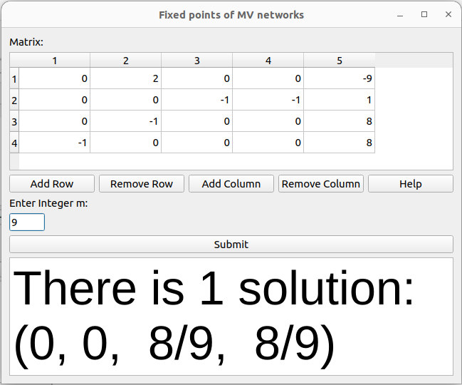
Figure 3. Screenshot of the app [Aye]

6. Application to the Model for Denitrification in Pseudomonas aeruginosa

In [ABL] the authors try to unveil the environmental factors that contribute to greenhouse gas N₂O accumulation, especially in Lake Erie (Laurentian Great Lakes, USA). Their model predicts the long-term behavior of the denitrification pathway, it has three Boolean external parameters (O₂, PO₄, NO₃), four Boolean variables ($PhoRB,PhoPQ,PmrA$,$Anr$), and eleven ternary variables ($NarXL$, $Dnr$, $NirQ$, $nar$, $nir$, $nor$, $nos$, $NO_{2}$, $NO$, $N_{2}O$, $N_{2}$). In our setting, we assume that they take values in $X_{2}$. The corresponding update rules in [ABL] are:

$f_{PhoRB}$	$=$	$\mathrm{neg}(PO_{4})$,	$f_{NarXL}$	$=$	$\min\{Anr,NO_{3}\}$,	$f_{NO}$	$=$	$\min\{NO_{2},nir\}$,
$f_{PhoPQ}$	$=$	$PhoRB$,	$f_{nir}$	$=$	$\max\{NirQ,\min\{Dnr,NO\}\}$,	$f_{N_{2}O}$	$=$	$\min\{NO,nor\}$,
$f_{PmrA}$	$=$	$\mathrm{neg}(PhoPQ)$,	$f_{nor}$	$=$	$\max\{NirQ,\min\{Dnr,NO\}\}$,	$f_{N_{2}}$	$=$	$\min\{N_{2}O,nos\}$,
$f_{Anr}$	$=$	$\mathrm{neg}(O_{2})$,	$f_{nos}$	$=$	$\min\{Dnr,NO\}$.

As we pointed out in our Introduction, they cannot accurately express four variables (${Dnr}$, ${NirQ}$, ${nar}$ and ${NO_{2}}$) using only the operators MAX, MIN and NOT (indicated with a $*$ in [ABL, Table 3]), and are then forced to show all the possible values in supplementary tables. From the transition tables of each of the 15 variables, they build a polynomial dynamical system and compute the fixed points of the system (with a software based on Gröbner basis computations) under the environmental conditions of interest that emerge after fixing the values of the external parameters.

To further show the strength of the tools we developed in this paper, we implemented their model in our setting. We can translate the functions shown above to operations with $\odot$ and $\oplus$ using Proposition 4. For the remaining functions, $f_{Dnr}$, $f_{NirQ}$, $f_{nar}$ and $f_{NO_{2}}$, we considered the supplementary tables in [ABL] without the smoothing process since the fixed points are not changed (see Lemma 14). For instance, the values for $NirQ$ are shown in Figure LABEL:fig:NirQ. We can see that the fourth transition $(NarXL=1,Dnr=0)\mapsto NirQ=\frac{1}{2}$ does not agree with the function $\max\{NarXL,Dnr\}$ in [ABL]. However, we can represent any multivalued function in our framework. There is always a standard alternative to do this by building the interpolation function in Theorem 10. In this case, there is a much better alternative: find a more intuitive and simple expression where $Dnr$ is an activator and $NarXL$ is a mild activator (see Motifs 1 and 4 in § 2.3). See Figure LABEL:fig:NirQ.