Second-order adiabatic expansions of heat and charge currents with nonequilibrium Green’s functions.

Sebastián E. Deghi,1 and Raúl A. Bustos-Marún1,2 1Instituto de Física Enrique Gaviola and Facultad de Matemática, Astronomía, Física y Computación, Universidad Nacional de Córdoba, Ciudad Universitaria, Córdoba, 5000, Argentina
2Facultad de Ciencias Químicas, Universidad Nacional de Córdoba, Ciudad Universitaria, Córdoba, 5000, Argentina
Abstract

Due to technological needs, nanoscale heat management, energy conversion and quantum thermodynamics have become key areas of research, putting heat pumps and nanomotors center stage. The treatment of these particular systems often requires the use of adiabatic expansions in terms of the frequency of the external driving or the velocity of some classical degree of freedom. However, due to the difficulty of getting the expressions, most works have only explored first-order terms. Despite this, adiabatic expansions have allowed the study of intriguing phenomena such as adiabatic quantum pumps and motors, or electronic friction. Here, we use nonequilibrium Green’s functions, within a Schwinger-Keldysh approach, to develop second-order expressions for the energy, heat, and charge currents. We illustrate, through two simple models, how the obtained formulas produce physically consistent results, and allow for the thermodynamic study of unexplored phenomena, such as second-order monoparametric pumping.

I Introduction

The conversion of heat into work (either mechanical or electrical) has been at the center of technological and scientific interest since the first studies of steam engines (Carnot et al., 1890). In the past decades, miniaturization has guided this interest toward micro- and nanoscale heat-to-work conversion (Benenti et al., 2017; Whitney et al., 2018; Bustos-Marún and Calvo, 2019; Zimbovskaya and Nitzan, 2020; Aligia et al., 2020; Pekola and Karimi, 2021; Alicki et al., 2021; Eglinton and Brandner, 2022; Arrachea, 2023). This was not only due to the fundamental questions posed by the new size scale (Esposito et al., 2015; Acciai et al., 2024), but also to practical reasons such as the need for efficient heat management of nanodevices. However, the nanoscale presents new challenges. On the one hand, the regions of interest now involved a finite number of particles, as opposed to classical thermodynamics. On the other hand, the explicit treatment of quantum mechanical effects often becomes unavoidable.

Importantly, nanoscale quantum machines (devices with strong quantum effects) require appropriate and efficient computational treatments. This is so, since processes with vastly different time scales may coexist there. Therefore, without any type of approximation, the calculations must then be carried out with a temporal resolution given by the fastest degrees of freedom (DOFs) but with total times determined by the slowest DOFs. This clearly makes numerical calculations highly inefficient. Even worse, sometimes contrasting theoretical approaches may be needed for the different DOFs.

A successful strategy followed in the past consisted of treating some slow DOFs classically (typically nuclear, mechanical, or external ones). In contrast, the fast DOFs are treated fully quantum (typically electrons or optical phonons). For nanoelectronic or nanoelectromechanical devices, the time scale separation also drives the establishment of steady-state currents which parametrically depend on the position and velocity of the slow DOFs. This situation is amenable to some kind of adiabatic approximation where the observable of interest is expanded in terms of the frequency of the external driving or the velocity of the classical DOFs. In this context, different theoretical approaches have been used including non-equilibrium Green’s functions (NEGF) (Mozyrsky et al., 2006; Pistolesi et al., 2008; Zazunov and Egger, 2010; Bode et al., 2011; Deghi et al., 2021), real-time diagrammatic approaches (Splettstoesser et al., 2006; Leijnse and Wegewijs, 2008; Calvo et al., 2017; Ribetto et al., 2021) (or similar approaches based on the adiabatic expansions of the system’s reduced density matrix (Dundas et al., 2009; Lin et al., 2019)), scattering formalism (Moskalets and Büttiker, 2004; Bennett et al., 2010; Bode et al., 2011), DFT-based calculations (Lü et al., 2015), and hierarchical equation of motion approaches (Erpenbeck et al., 2018; Rudge et al., 2023).

Within the context of quantum transport, adiabatic approximations up to the first order have allowed the treatment of fascinating phenomena such as adiabatic quantum pumping (Brouwer, 1998), adiabatic quantum motors(Bustos-Marún et al., 2013), negative friction coefficients (Bode et al., 2011; Preston et al., 2022), reciprocity breaking (Wächtler et al., 2021; Mehring et al., 2024), hysteresis (Kurnosov et al., 2022; Mehring et al., 2024), current-noise induced by thermal oscillations (Ribetto et al., 2023), etc. Regardless of the notable advances made, one may wonder about the unexplored phenomena that may await beyond first-order adiabatic treatments. In this sense, Kershaw et al. (Kershaw and Kosov, 2017, 2019) pioneered the second-order treatment of electric currents within a NEGF approach. However, a thermodynamically consistent second-order treatment of quantum machines necessarily requires addressing heat currents. Moreover, explicit expressions of the observables are desirable for numerical calculations, instead of implicit expressions that need to be developed for the cases of interest. In the present manuscript, we present the complete and explicit expressions, up to the second order of the adiabatic expansions of heat and charge currents. Our results are based on NEGFs within a Schwinger-Keldysh approach. The obtained formulas are general and restricted only by the assumption of time-independent self-energies.111It is important to highlight that this quite common assumption is not a limitation for a wide class of systems. For example, in a tight-binding approach, one can redefine the local system by adding the sites of the leads with time dependence (Cattena et al., 2014).

This manuscript is organized as follows. Sec. II presents the general theory based on the NEGF formalism. Having developed the theoretical tools, in Sec. III, we provide the second-order adiabatic expansion for charge, energy, and heat currents. Sec. IV contains two different models illustrating how the corrections for each order work and the usefulness of the expressions for thermodynamic analysis. In particular, the last example treats second-order quantum pumping, a phenomenon not previously described up to our knowledge. The examples also include a numerical verification of our formulas through the first law of thermodynamics. Finally, Sec. V comprises a summary and a brief discussion. In an effort not to overload the readers, all the nonessential comments and mathematical details lay in the Appendices from A to I.

II General theory

II.1 Generic Hamiltonian

To define the different parts of the system and their associated creation (annihilation) operators, we introduce the total Hamiltonian $H$ that describes the total system. It consists of a core region $S$ connected to several macroscopic reservoirs $\alpha$ (the leads). The core region, which typically has nanometric dimensions, will be referred to as the local system. The total Hamiltonian takes the form

$\displaystyle H$ $\displaystyle=\underset{\alpha}{\sum}H_{\alpha}+H_{S}+\underset{\alpha}{\sum}V_{\alpha},$

where $H_{S}$, in general, corresponds to a time-dependent local system, $H_{\alpha}$ describes the time-independent $\alpha$-lead, and the term $V_{\alpha}$ contains the time-independent interaction between the local system and the $\alpha$-lead. The Hamiltonian of the local system depends parametrically on time through a multidimensional vector $\overrightarrow{X}$, which describes the mechanical degrees of freedom. The local system’s Hamiltonian assumes the following form when the second quantization is applied

$\displaystyle H_{S}$ $\displaystyle=\underset{l,s}{\sum}h_{l,s}\left(\overrightarrow{X}\right)d_{l}^{\dagger}d_{s}.$ (1)

In the notation we have used, the operators $d_{l}^{\dagger}$ and $d_{l}$ create or annihilate, respectively, an electron within the local system. The Hamiltonians of the leads can be written as

$\displaystyle H_{\alpha}$ $\displaystyle=\underset{k}{\sum}\epsilon_{\alpha k}c_{\alpha k}^{\dagger}c_{\alpha k},$ (2)

where $\epsilon_{\alpha k}$ is the energy of the $\alpha$-lead in the state $k$, $c_{\alpha k}^{\dagger}$ creates an electron in the $\alpha$-lead with the state $k$, whereas the $c_{\alpha k}$ annihilates it. For simplicity, the index $k$ also includes the electron’s spin. Finally, the tunneling interaction describes the coupling between the local system and the $\alpha$-leads

$\displaystyle V_{\alpha}$ $\displaystyle=\underset{k,l}{\sum}\left(t_{\alpha k,l}c_{\alpha k}^{\dagger}d_{l}+t_{\alpha k,l}^{*}d_{l}^{\dagger}c_{\alpha k}\right),$

where $t_{\alpha k,l}$ are the tunneling amplitudes between the leads and the local system.

II.2 Dynamics of non-equilibrium open quantum systems

Within the context of the Schwinger-Keldysh approach for the NEGF formalism (Jauho et al., 1994; Maciejko, 2007; Haug and Jauho, 2008; Spicka et al., 2014; Odashima and Lewenkopf, 2017) we define the elements of the retarded and advanced Green’s functions, $\mathcal{G}^{R}$ and $\mathcal{G}^{A}$ respectively. For a system that evolves, not necessarily in an equilibrium process, from $t^{\prime}$ to $t$ times, they are

$\displaystyle\mathcal{G}_{l,s}^{R}\left(t,t^{\prime}\right)$ $\displaystyle=-\frac{i}{\hbar}\Theta\left(t-t^{\prime}\right)\left\langle\left\{d_{s}\left(t\right),d_{l}^{\dagger}\left(t^{\prime}\right)\right\}\right\rangle,$ (3)

and

$\displaystyle\mathcal{G}_{s,l}^{A}\left(t^{\prime},t\right)$ $\displaystyle=\left[\mathcal{G}_{l,s}^{R}\left(t,t^{\prime}\right)\right]^{*},$ (4)

where $\left\{\bullet,\bullet\right\}$ is the anticommutator and $\left\langle\bullet\right\rangle$ is the quantum expectation value.

For the states of the local system, the lesser Green’s function elements are given by

$\displaystyle\mathcal{G}_{l,s}^{<}\left(t,t^{\prime}\right)$ $\displaystyle=\frac{i}{\hbar}\left\langle d_{l}^{\dagger}\left(t^{\prime}\right)d_{s}\left(t\right)\right\rangle,$ (5)

whereas for the states that propagate between the local system and leads, the lesser Green’s function elements are

$\displaystyle\mathcal{G}_{\alpha k,l}^{<}\left(t,t^{\prime}\right)$ $\displaystyle=\frac{i}{\hbar}\left\langle c_{\alpha k}^{\dagger}\left(t^{\prime}\right)d_{l}\left(t\right)\right\rangle.$ (6)

Furthermore, the retarded and advanced self-energies are assumed to be stationary.222For our purposes, stationary implies that the self-energies only depend on the time difference $t-t^{\prime}$, which means that both $V_{\alpha}$ and $H_{\alpha}$ are independent of the mechanical degrees of freedom. The elements of the retarded self-energy for the $\alpha$-lead take the form

$\displaystyle\Sigma_{\alpha,l,s}^{R}\left(t,t^{\prime}\right)$ $\displaystyle=\underset{k}{\sum}t_{l,\alpha k}g_{\alpha k}^{R}\left(t,t^{\prime}\right)t_{\alpha k,s},$ (7)

where

$\displaystyle g_{\alpha k}^{R}\left(t,t^{\prime}\right)$ $\displaystyle=-\frac{i}{\hbar}\Theta\left(t-t^{\prime}\right)e^{-\frac{i}{\hbar}\epsilon_{\alpha k}\left(t-t^{\prime}\right)}.$ (8)

Hence, the elements of total retarded self-energy comprise the sum of all leads

$\displaystyle\Sigma_{l,s}^{R}\left(t,t^{\prime}\right)$ $\displaystyle=\underset{\alpha}{\sum}\Sigma_{\alpha,l,s}^{R}\left(t,t^{\prime}\right).$ (9)

To obtain the advanced self-energy, we calculate the adjoint of the retarded one

$\displaystyle\Sigma_{\alpha,s,l}^{A}\left(t^{\prime},t\right)$ $\displaystyle=\left[\Sigma_{\alpha,l,s}^{R}\left(t,t^{\prime}\right)\right]^{*}.$ (10)

Likewise, the elements of the lesser self-energy of the $\alpha$-lead are given by

$\displaystyle\Sigma_{\alpha,l,s}^{<}\left(t,t^{\prime}\right)$ $\displaystyle=\underset{k}{\sum}t_{l,\alpha k}g_{\alpha k}^{<}\left(t,t^{\prime}\right)t_{\alpha k,s},$ (11)

where

$\displaystyle g_{\alpha k}^{<}\left(t,t^{\prime}\right)$ $\displaystyle=\frac{2\pi i}{\hbar}f_{\alpha}\left(\epsilon_{\alpha k}\right)e^{-\frac{i}{\hbar}\epsilon_{\alpha k}\left(t-t^{\prime}\right)}.$ (12)

Here, $f_{\alpha}$ is the $\alpha$-lead’s Fermi-Dirac distribution. To conclude, the elements of the total lesser self-energy are

$\displaystyle\Sigma_{l,s}^{<}\left(t,t^{\prime}\right)$ $\displaystyle=\underset{\alpha}{\sum}\Sigma_{\alpha,l,s}^{<}\left(t,t^{\prime}\right).$

Given the essential operators, the next step is to delve into the quantum dynamics, which in Schwinger-Keldysh formalism is expressed by the integrodifferential Dyson equation in terms of the retarded Green’s function

$\displaystyle-i\hbar\partial_{t^{\prime}}\mathcal{G}^{R}\left(t,t^{\prime}\right)$ $\displaystyle=\delta\left(t-t^{\prime}\right)+\mathcal{G}^{R}\left(t,t^{\prime}\right)H_{S}\left(t^{\prime}\right)$ (13)
$\displaystyle+\int\mathcal{G}^{R}\left(t,t_{1}\right)\Sigma^{R}\left(t_{1},t^{\prime}\right)dt_{1}.$

Here, the Hamiltonian of the local system, retarded Green’s function and self-energy are given by Eqs. (1), (3) and (9), respectively.

At this point, we can apply many techniques to solve Eq. (13). One way is to use numerical methods (Kloss et al., 2021). Another one is to develop an adiabatic expansion of the observables. To carry out the latter technique, we must decompose the defined operators and Dyson’s equation into two-time scales, which is done through the use of a Wigner transform.

II.3 Adiabatic expansion for retarded Green’s function

The idea is to separate the fast microscopic dynamics, followed by the electrons, from the slow macroscopic changes, determined by the classical mechanical degrees of freedom. Once the time scales have been distinguished, a gradient expansion will be carried out on the slow variables. First of all, we have to define the following transform of time variables

$\displaystyle T$ $\displaystyle=\frac{t+t^{\prime}}{2},$ (14)
$\displaystyle\tau$ $\displaystyle=t-t^{\prime}.$ (15)

The time scale $T$ is called the slow variable, while $\tau$ is the fast variable. The Wigner transform for the retarded Green’s function is defined as

$\displaystyle\mathcal{\widetilde{G}}^{R}\left(T,\varepsilon\right)$ $\displaystyle=\int\mathcal{G}^{R}\left(t,t^{\prime}\right)e^{\frac{i}{\hbar}\varepsilon\tau}d\tau,$

whereas its inverse transformation is

$\displaystyle\mathcal{G}^{R}\left(t,t^{\prime}\right)$ $\displaystyle=\frac{1}{2\pi\hbar}\int\mathcal{\widetilde{G}}^{R}\left(T,\varepsilon\right)e^{-\frac{i}{\hbar}\varepsilon\tau}d\varepsilon.$

For the elements of the retarded self-energy described in Eq. (7), $\Sigma^{R}\left(t,t^{\prime}\right)\equiv\Sigma^{R}\left(\tau\right)$, the Wigner transform becomes a Fourier transform, where

$\displaystyle\Sigma^{R}\left(\varepsilon\right)$ $\displaystyle=$ $\displaystyle\int\Sigma^{R}\left(\tau\right)e^{\frac{i}{\hbar}\varepsilon\tau}d\tau,$

and

$\displaystyle\Sigma_{\alpha,l,s}^{R}\left(\varepsilon\right)$ $\displaystyle=\Delta_{\alpha,l,s}\left(\varepsilon\right)-i\Gamma_{\alpha,l,s}\left(\varepsilon\right).$ (16)

Here, the level-width functions $\Gamma_{\alpha,l,s}$ are given by333The definitions of the level-width functions may differ from that of other authors (Haug and Jauho, 2008; Kershaw and Kosov, 2019). Here, we followed the convention used in (Bode et al., 2011; Cattena et al., 2014; Deghi et al., 2021).

$\displaystyle\Gamma_{\alpha,l,s}\left(\varepsilon\right)$ $\displaystyle=\pi\underset{k}{\sum}\delta\left(\varepsilon-\epsilon_{\alpha k}\right)t_{l,\alpha k}t_{\alpha k,s}.$

The level-shift functions $\Delta_{\alpha,l,s}$ can be calculated from $\Gamma_{\alpha,l,s}$ using the Kramers-Kroning relation (Haug and Jauho, 2008). After applying the adjoint operator to Eq. (16) we get the advanced self-energy $\Sigma_{\alpha,l,s}^{A}$. For the elements of the lesser self-energy given in Eq. (11), their Wigner transform give

$\displaystyle\Sigma_{\alpha,l,s}^{<}\left(\varepsilon\right)$ $\displaystyle=2if_{\alpha}\left(\varepsilon\right)\Gamma_{\alpha,l,s}\left(\varepsilon\right).$ (17)

Given the operators in the energy domain, we must apply the Moyal product to Eq. (13), yielding (see Appendix A)

$\displaystyle 1$ $\displaystyle=-\frac{1}{2}i\hbar\partial_{T}\mathcal{\widetilde{G}}^{R}\left(T,\varepsilon\right)+\varepsilon\mathcal{\widetilde{G}}^{R}\left(T,\varepsilon\right)$
$\displaystyle-\mathcal{\widetilde{G}}^{R}\left(T,\varepsilon\right)e^{\frac{i\hbar}{2}\left(\overleftarrow{\partial}_{\varepsilon}\overrightarrow{\partial}_{T}-\overleftarrow{\partial}_{T}\overrightarrow{\partial}_{\varepsilon}\right)}\Sigma^{R}\left(\varepsilon\right)$ (18)
$\displaystyle-\mathcal{\widetilde{G}}^{R}\left(T,\varepsilon\right)e^{\frac{i\hbar}{2}\left(\overleftarrow{\partial}_{\varepsilon}\overrightarrow{\partial}_{T}-\overleftarrow{\partial}_{T}\overrightarrow{\partial}_{\varepsilon}\right)}\hat{H}_{S}\left(T\right),$

The above expression implies that the unknown retarded green’s function $\mathcal{\widetilde{G}}^{R}$ can be expressed as an infinite sum over its derivatives, which are also unknown in principle. To solve this, we have to implement an iterative approach (see Appendix B) which starts at zero-order by approximating $\mathcal{\widetilde{G}}^{R}$ by the adiabatic Green’s function $G^{R}$, defined as

$\displaystyle G^{R}$ $\displaystyle=\left[\varepsilon I-H_{S}\left(T\right)-\Sigma^{R}\left(\varepsilon\right)\right]^{-1}.$ (19)

The above adiabatic (or frozen) Green’s function $G^{R}$ is formally equal to $\mathcal{\widetilde{G}}^{R}\left(T,\varepsilon\right)$ in the limit of infinitely slow mechanical degrees of freedom, which constitute a form of the Born-Oppenheimer approximation.

By the chain rule, the slow-time $T$ derivatives of the Hamiltonian of the local system, up to the second order, are

$\displaystyle\partial_{T}H_{S}$ $\displaystyle=\stackrel{{\scriptstyle[}}{{\nu}}=1]{M}{\sum}\varLambda_{\nu}\dot{X}_{\nu},$ (20)
$\displaystyle\partial_{T}^{2}H_{S}$ $\displaystyle=\stackrel{{\scriptstyle[}}{{\mu}},\nu=1]{M}{\sum}\varLambda_{\mu\nu}\dot{X}_{\mu}\dot{X}_{\nu}+\stackrel{{\scriptstyle[}}{{\nu}}=1]{M}{\sum}\varLambda_{\nu}\ddot{X}_{\nu}.$ (21)

Here, $\dot{X}_{\nu}$ and $\ddot{X}_{\nu}$ are the time derivatives of the mechanical degree of freedom $\nu$, $\partial_{T}X_{\nu}$ and $\partial_{T}^{2}X_{\nu}$ respectively. Additionally, the elements of the matrices $\varLambda_{\nu}$ and $\varLambda_{\mu\nu}$ are given by

$\displaystyle\left[\varLambda_{\nu}\right]_{l,s}$ $\displaystyle=\frac{\partial h_{l,s}}{\partial X_{\nu}},$ $\displaystyle\left[\varLambda_{\mu\nu}\right]_{l,s}$ $\displaystyle=\frac{\partial^{2}h_{l,s}}{\partial X_{\mu}\partial X_{\nu}}.$

Then, applying the iterative method twice to second-order terms, the resulting retarded Green’s function takes the form

$\displaystyle\mathcal{\widetilde{G}}^{R}$ $\displaystyle\simeq G^{R}\left(T,\varepsilon\right)+\frac{i\hbar}{2}\stackrel{{\scriptstyle[}}{{\nu}}=1]{M}{\sum}\Omega_{1,\nu}^{R}\left(T,\varepsilon\right)\dot{X}_{\nu}$ (22)
$\displaystyle+\left(\frac{i\hbar}{2}\right)^{2}\left\{\stackrel{{\scriptstyle[}}{{\mu}},\nu=1]{M}{\sum}\Omega_{11,\mu\nu}^{R}\dot{X}_{\mu}\dot{X}_{\nu}+\stackrel{{\scriptstyle[}}{{\nu}}=1]{M}{\sum}\Omega_{2,\nu}^{R}\ddot{X}_{\nu}\right\}.$

To make the notation more compact, we have defined the following operators

$\displaystyle\Omega_{1,\nu}^{R}$ $\displaystyle=\Xi_{1}\left[G^{R},\varLambda_{\nu},G^{R}\right],$
$\displaystyle\Omega_{11,\mu\nu}^{R}$ $\displaystyle=\Xi_{11}\left[G^{R},K_{\mu\nu}^{R},G^{R}\right],$
$\displaystyle\Omega_{2,\nu}^{R}$ $\displaystyle=\frac{1}{2}\Xi_{2}\left[G^{R},\varLambda_{\nu},G^{R}\right].$

where we have also introduced the definitions

$\displaystyle K_{\mu\nu}^{R}$ $\displaystyle=\varLambda_{\mu}G^{R}\left(T,\varepsilon\right)\varLambda_{\nu}+\frac{1}{2}\varLambda_{\mu\nu},$

and

$\displaystyle\Xi_{1}\left[A,B,C\right]$ $\displaystyle=\left(\partial_{\varepsilon}A\right)BC-AB\left(\partial_{\varepsilon}C\right),$
$\displaystyle\Xi_{2}\left[A,B,C\right]$ $\displaystyle=\left(\partial_{\varepsilon}^{2}A\right)BC-2\left(\partial_{\varepsilon}A\right)B\left(\partial_{\varepsilon}C\right)$
$\displaystyle+AB\left(\partial_{\varepsilon}^{2}C\right),$
$\displaystyle\Xi_{11}\left[A,B,C\right]$ $\displaystyle=\Xi_{2}\left[A,B,C\right]-A\left(\partial_{\varepsilon}^{2}B\right)C.$

Take into account that the order to which the Planck’s constant is elevated is consistent with the order of the adiabatic expansion. In this sense, it can be used as a "book-keeping" parameter to keep track of the expansion order for a given term.

Finally, to calculate the advanced Green function, we use the relation

$\displaystyle\mathcal{\widetilde{G}}^{A}$ $\displaystyle=\left[\mathcal{\widetilde{G}}^{R}\left(T,\varepsilon\right)\right]^{\dagger}.$

II.4 Adiabatic expansion for lesser Green’s function

To find the Wigner’s transform of the lesser Green’s functions, Eqs. (5) and (6), we start with the relation (Maciejko, 2007; Haug and Jauho, 2008)

$\displaystyle\mathcal{G}^{<}\left(t,t^{\prime}\right)$ $\displaystyle=\iint\mathcal{G}^{R}\left(t,t_{1}\right)\Sigma^{<}\left(t_{1},t_{2}\right)\mathcal{G}^{A}\left(t_{2},t^{\prime}\right)dt_{1}dt_{2}.$

After applying the Wigner transform to both sides of the above formula and, afterwards, the Moyal product, we arrive at the expression

$\displaystyle\mathcal{\widetilde{G}}^{<}$ $\displaystyle=\mathcal{\widetilde{G}}^{R}\left(T,\varepsilon\right)e^{\frac{i\hbar}{2}\left(\overleftarrow{\partial}_{\varepsilon}\overrightarrow{\partial}_{T}-\overleftarrow{\partial}_{T}\overrightarrow{\partial}_{\varepsilon}\right)}\Sigma^{<}\left(\varepsilon\right)\times$
$\displaystyle e^{\frac{i\hbar}{2}\left(\overleftarrow{\partial}_{\varepsilon}\overrightarrow{\partial}_{T}-\overleftarrow{\partial}_{T}\overrightarrow{\partial}_{\varepsilon}\right)}\mathcal{\widetilde{G}}^{A}\left(T,\varepsilon\right).$ (23)

As we discussed for the retarded Green’s function, $\mathcal{\widetilde{G}}^{<}$ takes the form of a set of infinite sums (see Appendix C), where the elements of $\Sigma^{<}$ are given in Eq. (17). To solve this, we first insert in Eq. (23) the second-order expansion of the operators $\mathcal{\widetilde{G}}^{R}$ and $\mathcal{\widetilde{G}}^{A}$ derived before, and then we truncate the series at second order. This yields

$\displaystyle\mathcal{\widetilde{G}}^{<}$ $\displaystyle\simeq G^{<}\left(T,\varepsilon\right)+\frac{i\hbar}{2}\stackrel{{\scriptstyle[}}{{\nu}}=1]{M}{\sum}\Omega_{1,\nu}^{<}\left(T,\varepsilon\right)\dot{X}_{\nu}$ (24)
$\displaystyle+\left(\frac{i\hbar}{2}\right)^{2}\left\{\stackrel{{\scriptstyle[}}{{\mu}},\nu=1]{M}{\sum}\Omega_{11,\mu\nu}^{<}\dot{X}_{\mu}\dot{X}_{\nu}+\stackrel{{\scriptstyle[}}{{\nu}}=1]{M}{\sum}\Omega_{2,\nu}^{<}\ddot{X}_{\nu}\right\},$

Where the adiabatic lesser Green function is

$\displaystyle G^{<}$ $\displaystyle=G^{R}\left(T,\varepsilon\right)\Sigma^{<}\left(\varepsilon\right)G^{A}\left(T,\varepsilon\right),$

and the remaining operators are defined by

$\displaystyle\Omega_{1,\nu}^{<}$ $\displaystyle=\Xi_{1}\left[G^{R},\varLambda_{\nu},G^{<}\right]+\Xi_{1}\left[G^{<},\varLambda_{\nu},G^{A}\right],$
$\displaystyle\Omega_{11,\mu\nu}^{<}$ $\displaystyle=\Xi_{11}\left[G^{R},K_{\mu\nu}^{R},G^{<}\right]+\Xi_{11}\left[G^{<},K_{\mu\nu}^{A},G^{A}\right]$
$\displaystyle+\Xi_{11}\left[G^{R},\varLambda_{\mu}G^{<}\varLambda_{\nu},G^{A}\right],$
$\displaystyle\Omega_{2,\nu}^{<}$ $\displaystyle=\frac{1}{2}\left\{\Xi_{2}\left[G^{<},\varLambda_{\nu},G^{A}\right]+\Xi_{2}\left[G^{R},\varLambda_{\nu},G^{<}\right]\right\}.$

In the above expressions we have introduced the following term to compact the notation

$\displaystyle K_{\mu\nu}^{A}$ $\displaystyle=\varLambda_{\mu}G^{A}\left(T,\varepsilon\right)\varLambda_{\nu}+\frac{1}{2}\varLambda_{\mu\nu}.$

III Observables

We have already developed explicit formulas for evaluating up-to-second-order corrections to the adiabatic Green’s functions. In the following section, we will apply these results to obtain close expressions for the second-order adiabatic corrections of three observables of interest within quantum transport: charge, energy, and heat currents.

III.1 Charge current

For an $\alpha$-lead, the average charge current through it can be written as the mean value of the time derivative of the number operator $N_{\alpha}$

$\displaystyle I_{\alpha}$ $\displaystyle=-e\left\langle\dot{N}_{\alpha}\left(t\right)\right\rangle,$ (25)

where $N_{\alpha}=\underset{k}{\sum}c_{\alpha k}^{\dagger}c_{\alpha k},$ and $e$ is the modulus of the electron charge. Then, applying Ehrenfest’s theorem, the commutation relations for fermions, and using Eqs. (5) and (6) in Eq. (25), we get a formula for the charge current in terms of the lesser Green’s function

$\displaystyle I_{\alpha}$ $\displaystyle=2e\textrm{Re}\left\{\underset{k,l}{\sum}t_{\alpha k,l}\mathcal{G}_{l,\alpha k}^{<}\left(t,t\right)\right\}.$ (26)

To evaluate the time-dependent current $I_{\alpha}$, we must proceed in accord with the Langreth’s rules (van Leeuwen et al., 2006; Haug and Jauho, 2008), yielding

$\displaystyle I_{\alpha}$ $\displaystyle=2e\int\textrm{Re}\left\{\textrm{tr}\left[\mathcal{G}^{R}\left(t,t^{\prime}\right)\varSigma_{\alpha}^{<}\left(t^{\prime},t\right)\right.\right.$
$\displaystyle\left.\left.+\mathcal{G}^{<}\left(t,t^{\prime}\right)\varSigma_{\alpha}^{A}\left(t^{\prime},t\right)\right]\right\}dt^{\prime}.$ (27)

The next step is to insert the Wigner transform of the Green’s functions into Eq. (27) and make a gradient expansion, the resulting expression reads (see Appendix D)

$\displaystyle I_{\alpha}$ $\displaystyle=\frac{2e}{h}\stackrel{{\scriptstyle[}}{{N}}=0]{\infty}{\sum}\frac{\left(-1\right)^{N}}{N!}\int\textrm{Re}\left\{\textrm{tr}\left\{C_{\alpha,N}^{I}\right\}\right\}d\varepsilon,$ (28)

where

$\displaystyle C_{\alpha,N}^{I}$ $\displaystyle=\left(\frac{i\hbar}{2}\right)^{N}\left(\partial_{T}^{N}\mathcal{\widetilde{G}}^{R}\partial_{\varepsilon}^{N}\varSigma_{\alpha}^{<}+\partial_{T}^{N}\mathcal{\widetilde{G}}^{<}\partial_{\varepsilon}^{N}\varSigma_{\alpha}^{A}\right).$

It is important to highlight that, although this expression is exact, its explicit evaluation necessarily requires approximations. For this purpose, we will use the up-to-second-order adiabatic expansion of the Green’s functions found previously. After some algebra, one can find the up-to-second-order adiabatic expansion of the charge current, giving

$\displaystyle I_{\alpha}$ $\displaystyle\simeq I_{\alpha}^{\left(0\right)}+I_{\alpha}^{\left(1\right)}+I_{\alpha}^{\left(1,1\right)}+I_{\alpha}^{\left(2\right)}.$ (29)

The first two terms of the above expression are well known. The former, $I_{\alpha}^{\left(0\right)}$, is equivalent to Landauer’s formula, while the second one, $I_{\alpha}^{\left(1\right)}$, is the quantum pumping contribution to the charge current (Brouwer, 1998; Bode et al., 2011)

$\displaystyle I_{\alpha}^{\left(0\right)}$ $\displaystyle=-e\mathcal{N}_{\alpha}^{\left(0\right)},$ (30)
$\displaystyle I_{\alpha}^{\left(1\right)}$ $\displaystyle=-e\underset{\nu}{\sum}\mathcal{N}_{\alpha,\nu}^{\left(1\right)}\dot{X}_{\nu}.$ (31)

Here, we have introduced the terms

$\displaystyle\mathcal{N}_{\alpha}^{\left(0\right)}$ $\displaystyle=\int\mathcal{K}_{\alpha}^{\left(0\right)}\left(T,\varepsilon\right)d\varepsilon,$ $\displaystyle\mathcal{N}_{\alpha,\nu}^{\left(1\right)}$ $\displaystyle=\int\mathcal{K}_{\alpha,\nu}^{\left(1\right)}\left(T,\varepsilon\right)d\varepsilon.$

We acquire the preceding definition for practical purposes, which will be useful later, being the kernel’s integrals defined as

$\displaystyle\mathcal{K}_{\alpha}^{\left(0\right)}$ $\displaystyle=-\frac{2}{h}\textrm{Re}\left\{\textrm{tr}\left(\Phi_{\alpha}^{\left(0\right)}\right)\right\},$
$\displaystyle\mathcal{K}_{\alpha,\nu}^{\left(1\right)}$ $\displaystyle=\frac{1}{\pi}\textrm{Im}\left\{\textrm{tr}\left(\partial_{\varepsilon}G^{R}\varLambda_{\nu}\Phi_{\alpha}^{\left(0\right)}+\partial_{\varepsilon}G^{<}\varLambda_{\nu}\Phi_{\alpha}^{\left(1\right)}\right)\right\},$

where

$\displaystyle\Phi_{\alpha}^{\left(0\right)}$ $\displaystyle=G^{r}\varSigma_{\alpha}^{<}\left(\varepsilon\right)+G^{<}\varSigma_{\alpha}^{A}\left(\varepsilon\right),$ $\displaystyle\Phi_{\alpha}^{\left(1\right)}$ $\displaystyle=G^{A}\varSigma_{\alpha}^{A}\left(\varepsilon\right).$

The remaining terms in Eq. (29) constitute the second-order adiabatic terms of the charge current. These formulas can be written as

$\displaystyle I_{\alpha}^{\left(2\right)}$ $\displaystyle=-e\underset{\nu}{\sum}\mathcal{N}_{\alpha,\nu}^{\left(2\right)}\ddot{X}_{\nu},$ (32)
$\displaystyle I_{\alpha}^{\left(1,1\right)}$ $\displaystyle=-e\underset{\mu,\nu}{\sum}\mathcal{N}_{\alpha,\mu\nu}^{\left(1,1\right)}\dot{X}_{\mu}\dot{X}_{\nu}.$ (33)

The current derivatives $\mathcal{N}_{\alpha,\nu}^{\left(2\right)}=-\frac{1}{e}\frac{\partial I_{\alpha}}{\partial\ddot{X}_{\nu}}$ and $\mathcal{N}_{\alpha,\mu\nu}^{\left(1,1\right)}=-\frac{1}{e}\frac{\partial^{2}I_{\alpha}}{\partial\dot{X}_{\mu}\partial\dot{X}_{\nu}}$ are

$\displaystyle\mathcal{N}_{\alpha,\nu}^{\left(2\right)}$ $\displaystyle=\int\mathcal{K}_{\alpha,\nu}^{\left(2\right)}\left(T,\varepsilon\right)d\varepsilon,$ $\displaystyle\mathcal{N}_{\alpha,\mu\nu}^{\left(1,1\right)}$ $\displaystyle=\int\mathcal{K}_{\alpha,\mu\nu}^{\left(1,1\right)}\left(T,\varepsilon\right)d\varepsilon,$

The above kernels of integrals are

$\displaystyle\mathcal{K}_{\alpha,\nu}^{\left(2\right)}$ $\displaystyle=\frac{\hbar}{2\pi}\textrm{Re}\left\{\textrm{tr}\left\{\partial_{\varepsilon}^{2}G^{R}\varLambda_{\nu}\Phi_{\alpha}^{\left(0\right)}+\partial_{\varepsilon}^{2}G^{<}\varLambda_{\nu}\Phi_{\alpha}^{\left(1\right)}\right\}\right\},$
$\displaystyle\mathcal{K}_{\alpha,\mu\nu}^{\left(1,1\right)}$ $\displaystyle=\frac{\hbar}{\pi}\textrm{Re}\left\{\textrm{tr}\left\{\Phi_{\mu\nu}^{\left(2\right)}\Phi_{\alpha}^{\left(0\right)}+\Phi_{\mu\nu}^{\left(3\right)}\Phi_{\alpha}^{\left(1\right)}\right\}\right\},$

where

$\displaystyle\Phi_{\mu\nu}^{\left(2\right)}$ $\displaystyle=\partial_{\varepsilon}\left(\partial_{\varepsilon}G^{R}K_{\mu\nu}^{R}\right),$
$\displaystyle\Phi_{\mu\nu}^{\left(3\right)}$ $\displaystyle=\partial_{\varepsilon}\left(\partial_{\varepsilon}G^{R}\varLambda_{\mu}G^{<}\varLambda_{\nu}+\partial_{\varepsilon}G^{<}K_{\mu\nu}^{A}\right).$

III.2 Energy current

Analogous to the charge current, the energy current flowing in the $\alpha$-lead $\dot{E}_{\alpha}$ is defined as the mean value of the time derivative of the Hamiltonian of the $\alpha$-lead $H_{\alpha}$,

$\displaystyle\dot{E}_{\alpha}$ $\displaystyle=\left\langle\dot{H}_{\alpha}\left(t\right)\right\rangle.$ (34)

As we proceeded in the previous section for the charge current, we will apply Ehrenfest’s theorem, the commutation relations for fermions, and Eqs. (5) and (6) into Eq. (34). This gives

$\displaystyle\dot{E}_{\alpha}$ $\displaystyle=-2\textrm{Re}\left\{\underset{k,l}{\sum}\epsilon_{\alpha k}t_{\alpha k,l}\mathcal{G}_{l,\alpha k}^{<}\left(t,t\right)\right\}.$ (35)

Note that the essential difference between Eqs. (26) and (35) are the energy weights. This suggests employing a method akin to the charge currents strategy. However, despite using the same assumption, there are some subtle deviations from the reasoning for load currents, as illustrated in Appendix E. The final formula is

$\displaystyle\dot{E}_{\alpha}$ $\displaystyle=-2\textrm{Re}\left\{i\hbar\int\textrm{tr}\left[\mathcal{G}^{R}\left(t,t^{\prime}\right)\partial_{t^{\prime}}\varSigma_{\alpha}^{<}\left(t^{\prime},t\right)\right.\right.$
$\displaystyle\left.\left.+\mathcal{G}^{<}\left(t,t^{\prime}\right)\partial_{t^{\prime}}\varSigma_{\alpha}^{A}\left(t^{\prime},t\right)\right]\right\}dt^{\prime}.$ (36)

Unlike Eq. (27), the energy current formula shown above contains time derivatives over self-energies. Up to this point, the expression for energy current seems to be similar to the charge current. By applying the Wigner transform and the gradient expansion to Eq. (36) we arrive at (see Appendix F)

$\displaystyle\dot{E}_{\alpha}$ $\displaystyle=-\frac{2}{h}\stackrel{{\scriptstyle[}}{{N}}=0]{\infty}{\sum}\frac{\left(-1\right)^{N}}{N!}\int\varepsilon\textrm{Re}\left\{\textrm{tr}\left\{C_{\alpha,N}^{I}\right\}\right\}d\varepsilon$
$\displaystyle+\frac{2}{h}\stackrel{{\scriptstyle[}}{{N}}=0]{\infty}{\sum}\frac{\left(-1\right)^{N}}{N!}\int\textrm{Re}\left\{\textrm{tr}\left\{C_{\alpha,N}^{E}\right\}\right\}d\varepsilon.$ (37)

The additional term $C_{\alpha,N}^{E}$ is given by444Each of the $C_{\alpha,N}^{I}$ functions are dimensionless, whereas the $C_{\alpha,N}^{E}$ functions have energy units.

$\displaystyle C_{\alpha,N}^{E}$ $\displaystyle=\left(\frac{i\hbar}{2}\right)^{N+1}\left(\partial_{T}^{N+1}\mathcal{\widetilde{G}}^{R}\partial_{\varepsilon}^{N}\varSigma_{\alpha}^{<}+\partial_{T}^{N+1}\mathcal{\widetilde{G}}^{<}\partial_{\varepsilon}^{N}\varSigma_{\alpha}^{A}\right).$

After introducing the second-order adiabatic expansion of the retarded and lesser Green’s functions into Eq. (37), we get the adiabatic expansion up to the second-order of the energy current

$\displaystyle\dot{E}_{\alpha}$ $\displaystyle\simeq\dot{E}_{\alpha}^{\left(0\right)}+\dot{E}_{\alpha}^{\left(1\right)}+\dot{E}_{\alpha}^{\left(1,1\right)}+\dot{E}_{\alpha}^{\left(2\right)}.$ (38)

The adiabatic energy current is

$\displaystyle\dot{E}_{\alpha}^{\left(0\right)}$ $\displaystyle=\mathcal{\dot{\mathcal{E}}}_{\alpha}^{\left(0\right)}=\int\varepsilon\mathcal{K}_{\alpha}^{\left(0\right)}\left(T,\varepsilon\right)d\varepsilon,$ (39)

and its first correction $\dot{E}_{\alpha}^{\left(1\right)}$ takes the form

$\displaystyle\dot{E}_{\alpha}^{\left(1\right)}$ $\displaystyle=\underset{\nu}{\sum}\dot{\mathcal{E}}_{\alpha,\nu}^{\left(1\right)}\dot{X}_{\nu},$ (40)

where

$\displaystyle\mathcal{\dot{\mathcal{E}}}_{\alpha,\nu}^{\left(1\right)}$ $\displaystyle=\int\varepsilon\mathcal{K}_{\alpha,\nu}^{\left(1\right)}\left(T,\varepsilon\right)d\varepsilon.$

These terms are equivalent to those found previously by other authors, see for example Ludovico et al., 2016. However, the last two terms of Eq. (38) represent original expressions, to our knowledge. They read as

$\displaystyle\dot{E}_{\alpha}^{\left(2\right)}$ $\displaystyle=\underset{\nu}{\sum}\mathcal{\dot{\mathcal{E}}}_{\alpha,\nu}^{\left(2\right)}\ddot{X}_{\nu},$ (41)
$\displaystyle\dot{E}_{\alpha}^{\left(1,1\right)}$ $\displaystyle=\underset{\mu,\nu}{\sum}\mathcal{\dot{\mathcal{E}}}_{\alpha,\mu\nu}^{\left(1,1\right)}\dot{X}_{\mu}\dot{X}_{\nu},$ (42)

where the energy fluxes take the form

$\displaystyle\mathcal{\dot{\mathcal{E}}}_{\alpha,\nu}^{\left(2\right)}$ $\displaystyle=\int\varepsilon\mathcal{K}_{\alpha,\nu}^{\left(2\right)}\left(T,\varepsilon\right)d\varepsilon,$
$\displaystyle\mathcal{\dot{\mathcal{E}}}_{\alpha,\mu\nu}^{\left(1,1\right)}$ $\displaystyle=\int\varepsilon\mathcal{K}_{\alpha,\mu\nu}^{\left(1,1\right)}\left(T,\varepsilon\right)d\varepsilon.$

Note that, by comparing the adiabatic expansion of the charge current Eq. (29) with the energy one (Eq. 38), we recover, order-by-order, the straightforward interpretation of the energy current. It comes from the integration of all particles entering and leaving a given lead, but multiplied by the energy each particle carries. Mathematically this is a consequence of a subtle cancellation of the second term of Eq. (37).

III.3 Heat current

The heat current flowing through the $\alpha$-lead is the last observable we will study up to the second order. We can determine the expectation value of heat current based on the first law of thermodynamics (Esposito et al., 2015; Bustos-Marún and Calvo, 2019). The total energy gained or lost by a lead $\alpha$ is the sum of the heat and the work done by the particles being exchanged with the local system. In this way, the heat current $J_{\alpha}$ is given by

$\displaystyle J_{\alpha}$ $\displaystyle=\dot{E}_{\alpha}-\mu_{\alpha}\left\langle\dot{N}_{\alpha}\left(t\right)\right\rangle.$ (43)

The formal definition of Eq. (43) contains two mean values that we developed in subsections III.1 and III.2. Using the previous results, we can straightforwardly write the adiabatic expansion, up to the second order, of the heat current, just as we have done before

$\displaystyle J_{\alpha}$ $\displaystyle\simeq J_{\alpha}^{\left(0\right)}+J_{\alpha}^{\left(1\right)}+J_{\alpha}^{\left(1,1\right)}+J_{\alpha}^{\left(2\right)}.$

Employing Eqs. (30-33) and (39-42), we found

$\displaystyle J_{\alpha}^{\left(0\right)}$ $\displaystyle=\mathcal{J}_{\alpha}^{\left(0\right)},$ $\displaystyle J_{\alpha}^{\left(2\right)}$ $\displaystyle=\underset{\nu}{\sum}\mathcal{J}_{\alpha,\nu}^{\left(2\right)}\ddot{X}_{\nu},$
$\displaystyle J_{\alpha}^{\left(1\right)}$ $\displaystyle=\underset{\nu}{\sum}\mathcal{J}_{\alpha,\nu}^{\left(1\right)}\dot{X}_{\nu},$ $\displaystyle J_{\alpha}^{\left(1,1\right)}$ $\displaystyle=\underset{\mu,\nu}{\sum}\mathcal{J}_{\alpha,\mu\nu}^{\left(1,1\right)}\dot{X}_{\mu}\dot{X}_{\nu},$

where

$\displaystyle\mathcal{J}_{\alpha}^{\left(0\right)}$ $\displaystyle=\mathcal{\dot{\mathcal{E}}}_{\alpha}^{\left(0\right)}-\mu_{\alpha}\mathcal{N}_{\alpha}^{\left(0\right)},$ $\displaystyle\mathcal{\mathcal{J}}_{\alpha,\nu}^{\left(2\right)}$ $\displaystyle=\mathcal{\dot{\mathcal{E}}}_{\alpha,\nu}^{\left(2\right)}-\mu_{\alpha}\mathcal{N}_{\alpha,\nu}^{\left(2\right)},$
$\displaystyle\mathcal{\mathcal{J}}_{\alpha,\nu}^{\left(1\right)}$ $\displaystyle=\mathcal{\dot{\mathcal{E}}}_{\alpha,\nu}^{\left(1\right)}-\mu_{\alpha}\mathcal{N}_{\alpha,\nu}^{\left(1\right)},$ $\displaystyle\mathcal{J}_{\alpha,\mu\nu}^{\left(1,1\right)}$ $\displaystyle=\mathcal{\dot{\mathcal{E}}}_{\alpha,\mu\nu}^{\left(1,1\right)}-\mu_{\alpha}\mathcal{N}_{\alpha,\mu\nu}^{\left(1,1\right)}.$

Likewise, the above results can be written as integrals, giving

$\displaystyle\mathcal{\mathcal{J}}_{\alpha}^{\left(0\right)}$ $\displaystyle=\int\left(\varepsilon-\mu_{\alpha}\right)\mathcal{K}_{\alpha}^{\left(0\right)}\left(T,\varepsilon\right)d\varepsilon,$
$\displaystyle\mathcal{J}_{\alpha,\nu}^{\left(1\right)}$ $\displaystyle=\int\left(\varepsilon-\mu_{\alpha}\right)\mathcal{K}_{\alpha,\nu}^{\left(1\right)}\left(T,\varepsilon\right)d\varepsilon,$
$\displaystyle\mathcal{\mathcal{J}}_{\alpha,\nu}^{\left(2\right)}$ $\displaystyle=\int\left(\varepsilon-\mu_{\alpha}\right)\mathcal{K}_{\alpha,\nu}^{\left(2\right)}\left(T,\varepsilon\right)d\varepsilon,$
$\displaystyle\mathcal{J}_{\alpha,\mu\nu}^{\left(1,1\right)}$ $\displaystyle=\int\left(\varepsilon-\mu_{\alpha}\right)\mathcal{K}_{\alpha,\mu\nu}^{\left(1,1\right)}\left(T,\varepsilon\right)d\varepsilon.$

Thus far, we have offered a complete set of quantum transport observables to understand how the second-order corrections work. These results became a starting point to explore thermodynamic properties from a quantum point of view.

IV Models

In the previous sections, we formulated the theory of adiabatic expansions up to the second order for a set of fundamental observables. Now, we will evaluate the charge, energy, and heat currents for two different time-dependent devices. In studying these examples, we have three goals in mind. First, we want to illustrate the usage of the developed formulas and their utility for the thermodynamic analysis of nanomachines. Second, we want to test their validity by showing that the results they produce are physically reasonable. In particular, we will show that energy and particle number are conserved at all times and for all parameters in the order-by-order expansions (Bustos-Marún and Calvo, 2019). This involves the comparison of proven first-order formulas with the above-derived second-order terms. The first two points are shown in the first analyzed device, an atomic rotor in contact with two fixed leads (see Fig. 1). The second example consists of an oscillating quantum point contact (see Fig. 3). There we want to illustrate the kind of phenomena that can arise from the second-order terms of the observables. In this sense, we should recall that traditional adiabatic quantum pumping (Brouwer, 1998), requires the movement of at least two out-of-phase parameters. Instead, the studied device shows monoparametric pumping thanks to the second-order terms of charge currents, without requiring anharmonicities (Low et al., 2012) or quantum interference effects mediated by magnetic fields (Foa Torres, 2005).

IV.1 Driven atomic rotor

To model the atomic rotor we assume a minimal tight-binding model consisting of a one-site system attached to two identical conduction channels (the leads) through which an electrical current can flow. We will name each of them as $L$ and $R$. The isolated site is linked to the rotor and represents a quantum dot with a site energy $\epsilon_{d}$. Two semi-infinite tight-binding chains set up the leads, where $t_{L}$ and $t_{R}$ are the tunneling between them and the rotor (Deghi et al., 2021), as sketched in Fig. 1.

Refer to caption
Figure 1: Representation of a bidimensional atomic rotor attached to two leads.

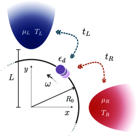
To keep matters simple, we assume only the hopping terms change with time, having a linear dependence on the distance between the rotor and the respective leads. Furthermore, we force the atomic rotor to follow a circular trajectory with a fixed radius $R_{0}$ and a given angular frequency $\omega$. Based on this outline, we arrive at (see Appendix G)

$\displaystyle t_{L}$ $\displaystyle=t_{\mathrm{max}}\left(1+a-a\sqrt{1+\beta\left(1-\sin\left(\omega t\right)\right)}\right),$ (44)
$\displaystyle t_{R}$ $\displaystyle=t_{\mathrm{max}}\left(1+a-a\sqrt{1+\beta\left(1-\cos\left(\omega t\right)\right)}\right),$ (45)

where $t_{\mathrm{max}}$ is the maximum (in absolute value) tunneling amplitude, $a$ sets the decay of the hopping terms with the distant between the dot and the leads, and

$\displaystyle\beta$ $\displaystyle=2\frac{R_{0}L}{\left(L-R_{0}\right)^{2}}.$

The description of the local system requires at least a three-site Hamiltonian, which includes the site energy of the central dot and the first sites of the leads. In this way, we circumvent the limitation mentioned earlier of time-independent self-energies $\Sigma^{r,a,<}\left(\varepsilon\right)$. The resulting adiabatic Green’s functions $G^{r,a,<}$, whose explicit forms can be found in (Deghi et al., 2021), do not commute, in general, with each other or $\Lambda$, as would be the case for a single site local system; see the example of Ref. Kershaw and Kosov, 2017. Thus, despite its simplicity, the analyzed example provides a challenging test for the developed formulas.

Once we set up the model, we apply the charge current formulas. For this purpose, we rewrite Eq. (29) (see Appendix G) for the current over the $L$-lead as

$\displaystyle I_{L}$ $\displaystyle=\varOmega_{I_{L}}^{\left(0\right)}+\varOmega_{I_{L}}^{\left(1\right)}\omega+\left(\varOmega_{I_{L}}^{\left(1,1\right)}+\varOmega_{I_{L}}^{\left(2\right)}\right)\omega^{2}.$ (46)

The term $\varOmega_{I_{L}}^{\left(0\right)}$ is the adiabatic contribution given by Eq. (30), $\varOmega_{I_{L}}^{\left(1\right)}$ is the first-order correction dictated by Eq. (31), and $\varOmega_{I_{L}}^{\left(1,1\right)}$ and $\varOmega_{I_{L}}^{\left(2\right)}$ stand for the second-order corrections of the charge current, given by Eqs. (32) and (33) respectively.

The procedure used for the charge current can be extended to the remaining studied observables. For example, the heat current formula takes the form

$\displaystyle J_{L}$ $\displaystyle=\varOmega_{J_{L}}^{\left(0\right)}+\varOmega_{J_{L}}^{\left(1\right)}\omega+\left(\varOmega_{J_{L}}^{\left(1,1\right)}+\varOmega_{J_{L}}^{\left(2\right)}\right)\omega^{2}.$ (47)

Despite their complexity, our goal is to ensure the validity of the formulas. To achieve this point, we will use the order-by-order energy conservation formulas for quantum transport (Bustos-Marún and Calvo, 2019). For our model, it reads

$\displaystyle Q_{J_{L}}^{\left(n\right)}-\frac{\delta\mu_{L}}{e}Q_{I_{L}}^{\left(n\right)}+Q_{J_{R}}^{\left(n\right)}-\frac{\delta\mu_{R}}{e}Q_{I_{R}}^{\left(n\right)}+W^{\left(n-1\right)}$ $\displaystyle=0.$ (48)

The above formula holds for any integer $n$, where $n$ represents the order of the adiabatic expansion of the quantity of interest, $W^{\left(n-1\right)}$ is the $n-1$ order of the work done by the rotor in a single cycle (see Appendix I), $Q_{J_{\alpha}}^{\left(n\right)}$ is the heat pumped per revolution of the rotor to the $\alpha$-lead, and $Q_{I_{\alpha}}^{\left(n\right)}$ is the pumped charge in a cycle. These quantities are evaluated as:

$\displaystyle W^{\left(n-1\right)}$ $\displaystyle=\stackrel{{\scriptstyle[}}{{0}}]{\tau}{\int}\overrightarrow{F}^{\left(n-1\right)}\cdot\overrightarrow{X}dt$ (49)
$\displaystyle Q_{J_{\alpha}}^{\left(n\right)}$ $\displaystyle=\stackrel{{\scriptstyle[}}{{0}}]{\tau}{\int}J_{\alpha}^{\left(n\right)}dt,$ (50)
$\displaystyle Q_{I_{\alpha}}^{\left(n\right)}$ $\displaystyle=\stackrel{{\scriptstyle[}}{{0}}]{\tau}{\int}I_{\alpha}^{\left(n\right)}dt.$ (51)

Here, $J_{\alpha}^{\left(n\right)}$ and $I_{\alpha}^{\left(n\right)}$ are defined in Section III, $\tau$ is the period of the movement, and $\overrightarrow{F}^{\left(n-1\right)}$ is the $n-1$ order of the adiabatic expansion of the electronic force $\overrightarrow{F}$. The latter is a vector whose components are defined by

$\displaystyle F_{\nu}\left(t\right)$ $\displaystyle=$ $\displaystyle-i\hbar\mathrm{Tr}\left[\Lambda_{\nu}\mathcal{G}^{<}\left(t,t\right)\right].$

It is important to highlight that the fulfillment of Eq. (48) with second-order corrections of the heat and charge currents involves the comparison of developed formulas with the well-known expressions for the zero and first-order electronic forces, $\overrightarrow{F}^{(0)}$ and $\overrightarrow{F}^{(1)}$, which can be found in Refs. (Bode et al., 2011; Deghi et al., 2021).

A further magnitude of significance is the total energy pumped to the $\alpha$-lead, which reads:

$\displaystyle Q_{\dot{E}_{\alpha}}^{\left(n\right)}$ $\displaystyle=Q_{J_{\alpha}}^{\left(n\right)}-\frac{\delta\mu_{L}}{e}Q_{I_{\alpha}}^{\left(n\right)}.$

Rewriting Eq. (48) using the above formula, we obtain a version of the first law of thermodynamics which relates the total energy of electrons flowing between leads and the mechanical work. However, in this version electron energy and mechanical work are related through the different orders of their adiabatic expansion.

Finally, charge conservation is another property that must be satisfied for every order and can easily be tested in the present model
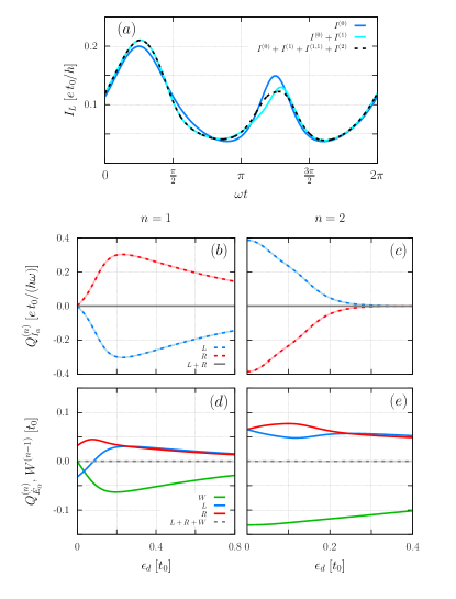
$\displaystyle Q_{I_{L}}^{\left(n\right)}+Q_{I_{R}}^{\left(n\right)}$ $\displaystyle=0.$

Fig. (2)-($a$) illustrates how the different orders of the charge current add up over one period of the rotor. Figs. 2-($b$) and 2-($c$) verify that the studied model satisfies charge conservation at every order for different values of the dot’s energy $\epsilon_{d}$. Figures 2-($d$) and 2-($e$) show, for different values of the dot’s energy $\epsilon_{d}$, order-by-order energy conservation for the first and second adiabatic corrections of the heat and charge currents.

We can also use the present example to highlight the importance of the developed formulas for the thermodynamic analysis of systems. For example, in Fig. 2 we can see that there is charge pumping in both orders [see $(b)$ and $(c)$] but energy pumping only occurs at first order. Note that for $n=1$ [Fig. $(d)$] and at $\epsilon_{d}$ close to 0, energy is on average going out of the left lead (blue line below zero) and entering into the right lead (red line above zero). On the contrary, at second-order of the currents [$n=2$, see $(e)$], energy coming from the external driving just dissipates through both leads (red and blue curves are always positive). Here, $W^{(1)}$ [geen line of Fig. 2 $(e)$] is the mechanical energy being dissipated by the electronic friction, see section I and Ref. Bustos-Marún and Calvo, 2019. The negative value of $W^{(0)}$ in Fig. $(d)$ (the work per cycle done by CIFs) is due to the sign choice of $\dot{X}\left(t\right)$, which in the present case implies that the system is being forced to act as a pump, not as a motor, see Ref. Bustos-Marún and Calvo, 2019. As a final remark, we note that for the present example second-order pumping points in a different direction than the first-order one. This implies that even small deviations from the adiabaticity should diminish the efficiency of adiabatic quantum pumps.

Refer to caption
Figure 2: $\boldsymbol{(a)}$ - Charge current (in units of $et_{0}/\hbar$) calculated up to different orders as function of $\omega t$. The different lines are: $I^{(0)}$ for blue, $I^{(0)}+I^{(1)}$ for cyan, and $I^{(0)}+I^{(1)}+I^{(2)}+I^{(1,1)}$ for the black dashed line. $\boldsymbol{(b)}$ and $\boldsymbol{(c)}$ - Pumped charge per cycle (in units of $et_{0}/(\hbar\omega)$) for the first and second orders. Red and blue dashed lines are $Q_{I_{R}}^{\left(n\right)}$ and $Q_{I_{L}}^{\left(n\right)}$ respectively, and the solid grey line is their sum. $\boldsymbol{(d)}$ and $\boldsymbol{(e)}$ - fulfillment of the order-by-order energy conservation (in units of $t_{0}$). The blue and red lines are $Q_{\dot{E}_{\alpha}}^{\left(n\right)}$ for $\alpha=L$ and $\alpha=R$ respectively, the green line is $W^{(n-1)}$, and the grey line shows the fulfillment of Eq. 48. For all calculations, the temperatures are $k_{B}T_{L}=k_{B}T_{R}=0.01$, the chemical potentials are $\delta\mu_{L}=0.1$ and $\delta\mu_{R}=-0.1$, $R_{0}=0.5$, $a=0.44$, $L=1$ and $t_{\mathrm{max}}=1$. For Fig. $(a)$, we fixed the quantum dot energy as $\epsilon_{d}=0.01$ and $\omega=0.1$.

IV.2 Oscillating QPC or STM’s tip

The system studied in this section consists of two conductors (not necessarily of the same materials) close enough to let charge particles tunnel from one to the other. Furthermore, the distance between the conductors oscillates at a given frequency $\omega$. This may represent different physical situations, which are in principle within experimental possibilities (Chen, 2021). Some of them are depicted in Fig. 3.
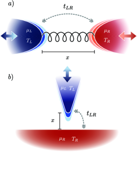
Refer to caption
Figure 3: Scheme of two possible physical systems described by the model of Sec. IV.2: $(a)$ an oscillating quantum point contact and $(b)$ a oscillating tip of a scanning tunneling microscope.

We modeled the different leads $L$ and $R$ using two distinct semi-infinite homogeneous tight-binding chains, as in the previous example, each characterized by a site energy and a hopping. The site energy of the lead $L$ ($R$) is $\epsilon_{0L}$ ($\epsilon_{0R}$) and its hopping is $t_{0L}$ ($t_{0R}$). The hopping between the leads $t_{LR}$ depends on their distance, exhibiting an exponential behavior (see Appendix H)

$\displaystyle t_{LR}$ $\displaystyle=t_{\mathrm{max}}e^{a\left(1-\frac{x}{x_{\mathrm{min}}}\right)},$ (52)

where $t_{\mathrm{max}}$ is the maximum tunneling amplitude, $a$ is the decay factor, $x$ is the distance between the leads, and $x_{\mathrm{min}}$ is the minimum value of $x$. Assuming a forced oscillatory movement and taking $\delta x+x_{\mathrm{min}}$ as the maximum length, the distance between leads yields

$\displaystyle x$ $\displaystyle=x_{\mathrm{min}}+\frac{\delta x}{2}\left(1-\cos\left(\omega t\right)\right).$ (53)

For the calculation of charge and heat currents, we rewrite the corresponding formulas just as we did in Eqs. (46) and (47). Moreover, for evaluating the fulfillment of the order-by-order energy conservation in the present model, we will also resort to the same definitions given in Eqs. (48), (49), and (51).

Refer to caption
Figure 4: $\boldsymbol{(a)}$ - Charge current (in units of $et_{0}/\hbar$) calculated up to different orders as function of $\omega t$. The different lines are: $I^{(0)}$ for blue, $I^{(0)}+I^{(1)}$ for cyan, and $I^{(0)}+I^{(1)}+I^{(2)}+I^{(1,1)}$ for the black dashed line. $\boldsymbol{(b)}$ - Second-order ($n=2$) pumped charges per cycle (in units of $et_{0}/(\hbar\omega)$) as a function of $\delta x/x_{\mathrm{min}}$. The blue dashed line belongs to the $L$-lead, the red one to the $R$-lead, and the grey line is the sum of both contributions. $\boldsymbol{(c)}$ - fulfillment of the order-by-order energy conservation law (in units of $t_{0}$) as a function of $\delta x/x_{\mathrm{min}}$. The blue and red lines are $Q_{\dot{E}_{\alpha}}^{\left(n\right)}$ for $\alpha=L$ and $\alpha=R$ respectively, the green line is $W^{(n-1)}$, and the grey line shows the fulfillment of Eq. 48. In all the plots we used: $k_{B}T_{L}=k_{B}T_{R}=0.01$, $\delta\mu_{L}=\delta\mu_{R}=0$, $t_{0L}=0.56$, $t_{0R}=1$, $\epsilon_{0L}=1$, $\epsilon_{0R}=0$, $a=0.5$, and $t_{\mathrm{max}}=0.99$. In Fig. $(a)$ we fixed $\delta x/x_{\mathrm{min}}=0.5$ and $\omega=0.1$.

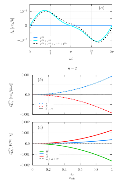
In Fig. 4 we evaluate the current for a system in equilibrium, i.e. $\left(\mu_{L},T_{L}\right)=\left(\mu_{R},T_{R}\right)$, with nonsymmetrical leads, which in this case means different energy sites $\epsilon_{0L}\neq\epsilon_{0R}$. There, the zero-order heat $J^{(0)}$ and charge currents $I^{(0)}$(adiabatic contributions) are zero, as can be seen for $I^{(0)}$ in Fig. 4-$(a)$ (blue solid line). Unlike the former example, the present one has only one independent mechanical degree of freedom. This implies a null contribution per cycle of the first-order heat and charge currents, $J^{(1)}$ and $I^{(1)}$, see Ref. Brouwer, 1998. Note in Fig. 4-$(a)$ that the cyan curve, $I^{(0)}+I^{(1)}$, is antisymmetric with respect to $I=0$. However, the second-order term may allow particles and heat to pump through the leads, even for a single-parameter system. Note that, the dotted black line in Fig. 4-$(a)$, $I^{(0)}+I^{(1)}+I^{(2)}+I^{(1,1)}$, is not antisymmetric for $I=0$ but has a shift towards negative values. In this example, it is then clear that second-order terms comprise the leading order for charge and heat pumping, exhibiting an unexplored form of quantum pumping.

In Figs. 4-$(b)$ and 4-$(c)$, we showed that the second-order term preserves, respectively, the total charge and energy of the complete system (local system plus the electron’s leads). From this figure, it is also interesting to note that, despite the charge current being pumped due to the second-order terms [see (b)], there is no heat pumping. In Figs. 4 (c) we can see that the heat per cycle $Q_{J}^{(2)}$ is positive for left and right leads, i.e., the external work ($W$) is dissipated as heat into the two leads. This mean that particles pumping from the left lead,555According to Eq. (25), the number of particles pumped per cycle is $-Q_{I_{L}}^{(2)}/e$. does not compensate for the external work ($W$) being dissipated as heat to this lead. This highlight, as in the previous example, the usefulness of the developed formulas for thermodynamic analysis.

For a symmetrical system (identical leads), we found (not shown in the manuscript) that no net particles move from one lead to another in the former configuration, even for the second-order correction. This behavior is expected since, due to inversion symmetry, there is no reason for the current to go in a preferential direction. In this sense, this also validates the second-order formulas.

V Conclusion

Throughout this work, we have presented expressions, based on NEGFs within a Schwinger-Keldysh approach, for the second-order adiabatic expansion of three different observables of quantum transport (energy, heat, and charge currents). To our knowledge, NEGF second-order expansions of heat and energy currents have not been treated before. Moreover, the explicit formulas for the observables are general and ready to be used in a wide range of systems. We only assumed that self-energies are time-independent, which is naturally accomplished for most quantum transport problems.

We have illustrated how the developed formulas produce physically consistent results (including order-by-order energy and particle conservation laws) using two simple models. We must emphasize that order-by-order energy conservation strictly involves the comparison of the here-developed expressions (second-order heat and charge currents) with a well-established first-order expression (first-order current-induced force). Moreover, we have shown in both examples how the developed formulas provide useful thermodynamical information about the devices. Additionally, in the second model, we have analyzed a phenomenon where second-order monoparametric pumping takes place. This provides a glimpse of the type of phenomenon that our expressions allow one to describe.

As for possible extensions of the present work, it would be interesting a deeper exploration of second-order phenomena and their potential use, as well as the development of similar formulas for other observables like current-induced forces (also known as electron wind forces (Hoffmann-Vogel, 2017)) or spin-transfer torque (Yang et al., 2021; Xiao et al., 2021; Wang et al., 2022; Tang and Cheng, 2024).

VI Acknowledgments

This work was financially supported by Consejo Nacional de Investigaciones Científicas y Técnicas (CONICET, PIP-2022-59241); Secretaría de Ciencia y Tecnología de la Universidad Nacional de Córdoba (SECyT-UNC, Proyecto Formar 2020); and Agencia Nacional de Promoción Científica y Tecnológica (ANPCyT, PICT-2018-03587).

Appendix A Wigner transform of Dyson’s equation

Eq. (13) is the equation of motion of the retarded Green’s function, usually called Dyson’s equation of motion. We can apply a Wigner transform to this expression. The first term on the right-hand side of Eq. (13) is the Dirac delta, whose Wigner transform is the identity. Before applying the Wigner transform to the second term, we need to rewrite it as

$\displaystyle A\left(t,t^{\prime}\right)$ $\displaystyle=\mathcal{G}^{R}\left(t,t^{\prime}\right)H_{s}\left(t^{\prime}\right)$
$\displaystyle=\int\mathcal{G}^{R}\left(t,t_{2}\right)h\left(t_{2},t^{\prime}\right)dt_{2},$ (54)

where

$\displaystyle h\left(t_{2},t^{\prime}\right)$ $\displaystyle=H_{S}\left(t_{2}\right)\delta\left(t_{2}-t^{\prime}\right).$

Now, we can apply the Wigner transform to $A\left(t,t^{\prime}\right)$, by using the Moyal product (Maciejko, 2007), yielding

$\displaystyle\widetilde{A}$ $\displaystyle=\mathcal{\widetilde{G}}^{R}\left(T,\varepsilon\right)e^{\frac{i\hbar}{2}\left(\overleftarrow{\partial}_{\varepsilon}\overrightarrow{\partial}_{T}-\overleftarrow{\partial}_{T}\overrightarrow{\partial}_{\varepsilon}\right)}\hat{H}_{S}\left(T\right).$ (55)

where we used $\widetilde{h}\left(T,\varepsilon\right)=H_{s}\left(T\right)$. The exponential operator is interpreted as usual in terms of the Maclaurin series of the exponential function, i.e., $e^{\hat{o}}=\sum_{n}\frac{\hat{o}^{n}}{n!}$ The arrows in the exponential indicate the direction in which the derivatives should be applied. For example, the symbol $\overrightarrow{\partial}_{\varepsilon}$ means: derivative with respect to $\varepsilon$ of the function to the right, $\hat{H}_{S}$ in the above case, while $\overleftarrow{\partial}_{\varepsilon}$ is the same but the derivative should be applied to the function to the left, $\mathcal{\widetilde{G}}^{R}\left(T,\varepsilon\right)$ in the above case.

The third term of Eq. (13),

$\displaystyle B\left(t,t^{\prime}\right)$ $\displaystyle=\int\mathcal{G}^{R}\left(t,t_{1}\right)\Sigma^{R}\left(t_{1},t^{\prime}\right)dt_{1},$

can also be Wigner transformed by using the Moyal product, giving

$\displaystyle\widetilde{B}$ $\displaystyle=\mathcal{\widetilde{G}}^{R}\left(T,\varepsilon\right)e^{\frac{i\hbar}{2}\left(\overleftarrow{\partial}_{\varepsilon}\overrightarrow{\partial}_{T}-\overleftarrow{\partial}_{T}\overrightarrow{\partial}_{\varepsilon}\right)}\Sigma^{R}\left(\varepsilon\right).$ (56)

To deal with the right-hand side of Eq. (13) we need to first apply the chain rule,

$\displaystyle\partial_{t^{\prime}}\mathcal{G}^{R}$ $\displaystyle=\frac{1}{2}\partial_{T}\mathcal{G}^{R}-\partial_{\tau}\mathcal{G}^{R},$

where $T$ and $\tau$ are defined in Eqs. (14) and (15) respectively. Then, after Wigner transform it we obtained

$\displaystyle\widetilde{\left(\partial_{t^{\prime}}\mathcal{G}^{r}\right)}$ $\displaystyle=\frac{1}{2}\partial_{T}\mathcal{\widetilde{G}}^{R}\left(T,\varepsilon\right)+\frac{i\varepsilon}{\hbar}\mathcal{\widetilde{G}}^{R}\left(T,\varepsilon\right),$

where we used the fact that Green’s functions have compact support in the energy domain. The final result of all the above is Eq. (18) of the main text.

In Eqs. (55) and (56) we used a compact notation, based on a exponential operator. However, the same equations can also be written as two infinite sums

$\displaystyle\widetilde{A}$ $\displaystyle=\stackrel{{\scriptstyle[}}{{N}}=0]{\infty}{\sum}\frac{1}{N!}\left(\frac{i\hbar}{2}\right)^{N}C_{N}^{A}\left(T,\varepsilon\right),$

and

$\displaystyle\widetilde{B}$ $\displaystyle=\stackrel{{\scriptstyle[}}{{N}}=0]{\infty}{\sum}\frac{1}{N!}\left(\frac{i\hbar}{2}\right)^{N}C_{N}^{B}\left(T,\varepsilon\right),$

where

$\displaystyle C_{N}^{A}$ $\displaystyle=\stackrel{{\scriptstyle[}}{{j}}=0]{N}{\sum}\left(-1\right)^{N-j}\binom{N}{j}\partial_{T}^{N-j}\partial_{\varepsilon}^{j}\mathcal{\widetilde{G}}^{R}\partial_{T}^{j}\partial_{\varepsilon}^{N-j}H_{s},$ (57)
$\displaystyle C_{N}^{B}$ $\displaystyle=\stackrel{{\scriptstyle[}}{{j}}=0]{N}{\sum}\left(-1\right)^{N-j}\binom{N}{j}\partial_{T}^{N-j}\partial_{\varepsilon}^{j}\mathcal{\widetilde{G}}^{R}\partial_{T}^{j}\partial_{\varepsilon}^{N-j}\Sigma^{R}.$ (58)

On the one hand, the slow time $T$ only affects the local system, according to our assumption. Therefore, the dynamics of the leads only depends on the energy $\varepsilon$. On the other hand, the Hamiltonian of the local system $H_{s}$ only depends on $T$ and not on $\varepsilon$. Then

$\displaystyle\partial_{\varepsilon}^{N-j}H_{s}$ $\displaystyle=0\;\forall N-1>j\geq 0.$ (59)
$\displaystyle\partial_{T}^{j}\Sigma^{R}$ $\displaystyle=0\;\forall N\geq j>1.$ (60)

This can be used in Eq. (18) of the main text to obtain a simpler expression. The results is

$\displaystyle 1$ $\displaystyle=-\frac{i\hbar}{2}\partial_{T}\mathcal{\widetilde{G}}^{R}+\varepsilon\mathcal{\widetilde{G}}^{R}-\stackrel{{\scriptstyle[}}{{N}}=0]{\infty}{\sum}\frac{1}{N!}\left(\frac{i\hbar}{2}\right)^{N}C_{N}.$ (61)

where we have introduced Eqs. (59) and (60) into Eqs. (57) and (58) respectively, and we have defined

$\displaystyle C_{N}$ $\displaystyle=\left(-1\right)^{N}\partial_{T}^{N}\mathcal{\widetilde{G}}^{R}\partial_{\varepsilon}^{N}\Sigma^{R}+\partial_{\varepsilon}^{N}\mathcal{\widetilde{G}}^{R}\partial_{T}^{N}H_{s}.$

The zero and first order terms of last expression can be compared with Eq. 20 of Ref. Bode et al., 2012.

Appendix B Adiabatic expansion for retarded Green’s function

The adiabatic retarded Green function, given in Eq. (19), satisfies the condition

$\displaystyle\left[G^{R}\left(T,\varepsilon\right)\right]^{-1}$ $\displaystyle=\varepsilon I-H_{s}\left(T\right)-\Sigma^{R}\left(T,\varepsilon\right).$ (62)

Then, the derivative of $G^{R}$ with respect to $\varepsilon$ gives

$\displaystyle\partial_{\varepsilon}G^{R}$ $\displaystyle=-G^{r}\left(1-\partial_{\varepsilon}\Sigma^{R}\right)G^{r}.$ (63)

where we used $\partial A=-A\partial\left[A^{-1}\right]A$.

Next, we have to change the sequence of the terms in the Eq. (61) to introduce the retarded Green’s function and its derivative, given in Eqs. (19) and (63). Then, using the slow-time derivative, Eqs. (20), and multiplying the adiabatic retarded Green’s function on both sides of the obtained equation, the resulting expression takes the form

$\displaystyle\mathcal{\widetilde{G}}^{R}$ $\displaystyle=G^{R}+\frac{i\hbar}{2}\stackrel{{\scriptstyle[}}{{\nu}}=1]{M}{\sum}\partial_{\varepsilon}\Sigma^{R}\varLambda_{\nu}G^{R}\dot{X}_{\nu}$ (64)
$\displaystyle-\frac{i\hbar}{2}\partial_{T}\mathcal{\widetilde{G}}^{R}\left[G^{R}\right]^{-1}\partial_{\varepsilon}G^{R}+\stackrel{{\scriptstyle[}}{{N}}=2]{\infty}{\sum}\frac{1}{N!}\left(\frac{i\hbar}{2}\right)^{N}C_{N}.$

Importantly, no approximations have been made in Eq. (64). Therefore, as long as the adiabatic expansion is valid (the series is convergent), the equation provides the exact evolution of $\mathcal{\widetilde{G}}^{R}$ along a path driven by the mechanical degrees of freedom $X_{\mu}$. However, note that $\mathcal{\widetilde{G}}^{R}$ (the exact retarded Green’s function) depends in turns on the time derivative of $\mathcal{\widetilde{G}}^{R}$, which is not known. In principle, the only retarded Green’s function known in advance is the adiabatic one, $G^{r}$. To solve this, one applies the iterative method twice. This consists of replacing $\mathcal{\widetilde{G}}^{R}$ on the right hand side by a first approximation ($G^{r}$), then using the resulting Green function to improve the approximation of $\mathcal{\widetilde{G}}^{R}$ on the right hand side, and so on. During this iterative process one identify terms of different orders given by the order of the derivatives with respect to $X_{\mu}$ and cut the infinite series at a given order (second order in our case). Note that the order also coincide with the exponent of $\hbar$ or the exponent of the driving frequency $\omega$ for the case $X_{\mu}\propto\cos\left(\omega t\right)$. By using this method we arrive, after some algebra, at Eq. (22) of the main text.

Appendix C Adiabatic expansion for lesser Green’s function

Starting from Eq. (23), which gives the lesser Green’s function Wigner transforms in close notation, we can write its gradient expansion as a double infinite sum

$\displaystyle\mathcal{\widetilde{G}}^{<}$ $\displaystyle=\stackrel{{\scriptstyle[}}{{N}},K=0]{\infty}{\sum}\frac{1}{N!K!}\left(\frac{i\hbar}{2}\right)^{N+K}W_{N,K}^{<}\left(T,\varepsilon\right),$ (65)

where we have introduced the nested definition

$\displaystyle W_{N,K}^{<}$ $\displaystyle=\stackrel{{\scriptstyle[}}{{j}}=0]{N}{\sum}\stackrel{{\scriptstyle[}}{{l}}=0]{K}{\sum}\left(-1\right)^{N}\binom{N}{j}\binom{K}{l}\partial_{T}^{N-j}\partial_{\varepsilon}^{j}\mathcal{\widetilde{G}}^{R}C_{j,l}^{N,K}$

and

$\displaystyle C_{j,l}^{N,K}$ $\displaystyle=\left(-1\right)^{j+l}\partial_{T}^{j}\partial_{\varepsilon}^{N-j}\left\{\partial_{T}^{K-l}\partial_{\varepsilon}^{l}\Sigma^{<}\partial_{T}^{l}\partial_{\varepsilon}^{K-l}\mathcal{\widetilde{G}}^{A}\right\}.$

The aforementioned expression is obtained by straightforwardly making use of the Moyal product twice.

The lesser self-energy is not time-dependent, since we have assumed that the retarded self-energy is not controlled by the slow time. This implies

$\displaystyle\partial_{T}^{K-l}\Sigma^{<}$ $\displaystyle=0\;\forall N-l\neq 0,$ (66)
$\displaystyle\partial_{T}^{j-m}\Sigma^{<}$ $\displaystyle=0\;\forall j-m\neq 0.$ (67)

Putting Eqs. (66) and (67) in Eq. (65), result in the simplified expression

$\displaystyle\mathcal{\widetilde{G}}^{<}$ $\displaystyle=\stackrel{{\scriptstyle[}}{{Q}}=0]{\infty}{\sum}\frac{1}{Q!}\left(\frac{i\hbar}{2}\right)^{Q}W_{Q}^{<}\left(T,\varepsilon\right),$ (68)

where

$\displaystyle W_{Q}^{<}$ $\displaystyle=\stackrel{{\scriptstyle[}}{{q}}=0]{Q}{\sum}\stackrel{{\scriptstyle[}}{{s}}=0]{q}{\sum}\stackrel{{\scriptstyle[}}{{j}}=0]{Q-q}{\sum}\left(-1\right)^{q}\binom{Q}{q+j}\binom{q+j}{j}\binom{q}{s}C_{q,j}^{Q},$

and

$\displaystyle C_{q,j}^{Q}$ $\displaystyle=\partial_{T}^{q}\partial_{\varepsilon}^{j}\mathcal{\widetilde{G}}^{R}\partial_{\varepsilon}^{Q-\left(j+s\right)}\Sigma^{<}\partial_{\varepsilon}^{s}\partial_{T}^{Q-q}\mathcal{\widetilde{G}}^{A}.$

The zero and first-order terms of Eq. (68) coincide with Eq. 25 of Ref. Bode et al., 2012 and Eq. 3 of Ref. Bode et al., 2011, once the iterative method explained in the previous section is applied. The result up to the second order is shown in Eq. (24) of the main text.

Appendix D Adiabatic expansion for charge currents

We start by rewriting Eq. (27) as

$\displaystyle I_{\alpha}$ $\displaystyle=2e\textrm{Re}\left\{\textrm{tr}\left[F_{\alpha}\left(t\right)\right]\right\},$ (69)

where the auxiliary operator $F_{\alpha}$ is defined by

$\displaystyle F_{\alpha}$ $\displaystyle=\int\left[\mathcal{G}^{R}\left(t,t^{\prime}\right)\varSigma_{\alpha}^{<}\left(t^{\prime},t\right)\right.$ (70)
$\displaystyle\left.+\mathcal{G}^{<}\left(t,t^{\prime}\right)\varSigma_{\alpha}^{A}\left(t^{\prime},t\right)\right]dt^{\prime}$

Now, our goal is to transform the $F_{\alpha}$ operator to the energy domain and then apply the inverse Wigner transform. This allows us to recover the charge current in the time domain written as an integral with a kernel in the energy domain. To carry out his technique, we start with the relationship between $F_{\alpha}$ and its Wigner transform $\widetilde{F}_{\alpha}$, whose formula takes the form

$\displaystyle F_{\alpha}$ $\displaystyle=\frac{1}{2\pi\hbar}\int\widetilde{F}_{\alpha}\left(T,\varepsilon\right)d\varepsilon.$ (71)

The next step is to put the gradient expansion in effect over Eq. (70), leading to

$\displaystyle\widetilde{F}_{\alpha}$ $\displaystyle=\stackrel{{\scriptstyle[}}{{N}}=0]{\infty}{\sum}\stackrel{{\scriptstyle[}}{{j}}=0]{N}{\sum}\frac{1}{N!}\left(-\frac{i\hbar}{2}\right)^{N}\binom{N}{j}C_{\alpha,N,j}^{F}\left(T,\varepsilon\right),$ (72)

where

$\displaystyle C_{\alpha,N,j}^{F}$ $\displaystyle=\left(-1\right)^{j}\partial_{T}^{N-j}\partial_{\varepsilon}^{j}\mathcal{\widetilde{G}}^{R}\partial_{T}^{j}\partial_{\varepsilon}^{N-j}\varSigma_{\alpha}^{<}$
$\displaystyle+\left(-1\right)^{j}\partial_{T}^{N-j}\partial_{\varepsilon}^{j}\mathcal{\widetilde{G}}^{<}\partial_{T}^{j}\partial_{\varepsilon}^{N-j}\varSigma_{\alpha}^{A}.$

As we have mentioned, we assumed that the leads are unaffected by the slow time variation. For such reason. Therefore, the following rules hold

$\displaystyle\partial_{T}^{j}\varSigma_{\alpha}^{A}$ $\displaystyle=0\;\forall N\geq j\geq 1,$ (73)
$\displaystyle\partial_{T}^{j}\varSigma_{\alpha}^{<}$ $\displaystyle=0\;\forall N\geq j\geq 1.$ (74)

Putting Eqs. (73) and (74) in Eq. (72), the Wigner transform of the $F_{\alpha}$ operator reads

$\displaystyle\widetilde{F}_{\alpha}$ $\displaystyle=\stackrel{{\scriptstyle[}}{{N}}=0]{\infty}{\sum}\frac{1}{N!}\left(-\frac{i\hbar}{2}\right)^{N}C_{\alpha,N}^{F}\left(T,\varepsilon\right),$ (75)

where

$\displaystyle C_{\alpha,N}^{F}$ $\displaystyle=\partial_{T}^{N}\mathcal{\widetilde{G}}^{R}\partial_{\varepsilon}^{N}\varSigma_{\alpha}^{<}+\partial_{T}^{N}\mathcal{\widetilde{G}}^{<}\partial_{\varepsilon}^{N}\varSigma_{\alpha}^{A}.$

To get the desired result, we must first plug the last equation into Eq. (71) and then into Eq. (69), leading to the formula outlined in Eq. (28).

Appendix E Energy current main formula

Taking Eq. (35) as a starting point, we intend to get an expression of the energy current in terms of self-energies, which lets us identify the leads. The quoted formula can be read as the product of the hooping between the local system and the leads, with those elements of the lesser Green’s function that connect the local system and leads, given by Eq. (6). However, we want to express the energy current in terms of the Green’s functions and self-energies of the local system only, Eq. (5). For this purpose, we will use the Keldysh technique and the Langreth theorem of analytic continuation to achieve this goal (Maciejko, 2007; van Leeuwen et al., 2006). The mean result is

$\displaystyle J_{\alpha}$ $\displaystyle=-2\textrm{Re}\left\{\int\mathcal{J}_{\alpha}\left(t,t^{\prime}\right)dt^{\prime}\right\},$

where

$\displaystyle\mathcal{J}_{\alpha}$ $\displaystyle=\underset{l,s}{\sum}\left(\mathcal{G}_{l,s}^{R}\left(t,t^{\prime}\right)f_{\alpha,s,l}^{<}\left(t^{\prime},t\right)+\mathcal{G}_{l,s}^{<}\left(t,t^{\prime}\right)f_{\alpha,s,l}^{A}\left(t^{\prime},t\right)\right).$

Here, $\mathcal{G}_{l,s}^{A}$ are the elements of the retarded Green’s function given in Eq. (3), and $\mathcal{G}_{l,s}^{<}$ are the lesser Green’s function specified in Eq. (5). In addition, we have introduced the following auxiliary functions

$\displaystyle f_{\alpha,s,l}^{<}$ $\displaystyle=\underset{k}{\sum}\epsilon_{\alpha k}t_{s,\alpha k}g_{\alpha k}^{<}\left(t^{\prime},t\right)t_{\alpha k,l},$ (76)
$\displaystyle f_{\alpha,s,l}^{A}$ $\displaystyle=\underset{k}{\sum}\epsilon_{\alpha k}t_{s,\alpha k}g_{\alpha k}^{A}\left(t^{\prime},t\right)t_{\alpha k,l}.$ (77)

As you can notice, these propagators satisfy the differential equations:

$\displaystyle\left(i\hbar\frac{\partial}{\partial t^{\prime}}-\epsilon_{\alpha k}\right)g_{\alpha k}^{<}\left(t^{\prime},t\right)$ $\displaystyle=0,$ (78)
$\displaystyle\left(i\hbar\frac{\partial}{\partial t^{\prime}}-\epsilon_{\alpha k}\right)g_{\alpha k}^{A}\left(t^{\prime},t\right)$ $\displaystyle=\delta\left(t^{\prime}-t\right).$ (79)

Moreover, and following our assumptions, we also have:

$\displaystyle\partial_{t^{\prime}}\left(t_{s,\alpha k}t_{\alpha k,l}\right)$ $\displaystyle=0.$

Then, putting Eqs. (78) and (79) into Eqs. (76) and (77), respectively, and using the previous condition, we arrive at

$\displaystyle f_{\alpha,s,l}^{<}$ $\displaystyle=\partial_{t^{\prime}}\varSigma_{\alpha,s,l}^{<}\left(t^{\prime},t\right),$
$\displaystyle f_{\alpha,s,l}^{A}$ $\displaystyle=\partial_{t^{\prime}}\varSigma_{\alpha,s,l}^{A}\left(t^{\prime},t\right)+\underset{k}{\sum}t_{s,\alpha k}\delta\left(t^{\prime}-t\right)t_{\alpha k,l}.$

Note that we have used the definitions of the self-energies given in Eqs. (10) and (11). The last equations allow us to write the following

$\displaystyle\mathcal{J}_{\alpha}$ $\displaystyle=\mathcal{J}_{\alpha}^{\left(0\right)}\left(t,t^{\prime}\right)+\mathcal{J}_{\alpha}^{\left(1\right)}\left(t,t^{\prime}\right),$

where

$\displaystyle\mathcal{J}_{\alpha}^{\left(A\right)}$ $\displaystyle=\textrm{tr}\left\{\mathcal{G}^{R}\left(t,t^{\prime}\right)\varSigma_{\alpha}^{0}\right\}\delta\left(t^{\prime}-t\right),$
$\displaystyle\mathcal{J}_{\alpha}^{\left(B\right)}$ $\displaystyle=\textrm{tr}\left\{\mathcal{G}^{R}\left(t,t^{\prime}\right)\partial_{t^{\prime}}\varSigma_{\alpha}^{<}\left(t^{\prime},t\right)+\mathcal{G}^{<}\left(t,t^{\prime}\right)\partial_{t^{\prime}}\varSigma_{\alpha}^{A}\left(t^{\prime},t\right)\right\}.$

For compactness, we have defined above the operator

$\displaystyle\varSigma_{\alpha,s,l}^{0}$ $\displaystyle=\underset{k}{\sum}t_{s,\alpha k}t_{\alpha k,l}.$

With this, the energy current takes the form

$\displaystyle J_{\alpha}$ $\displaystyle=J_{\alpha}^{\left(A\right)}+J_{\alpha}^{\left(B\right)},$

where

$\displaystyle J_{\alpha}^{\left(A\right)}$ $\displaystyle=-2\textrm{Re}\left\{\int\mathcal{J}_{\alpha}^{\left(A\right)}\left(t,t^{\prime}\right)dt^{\prime}\right\},$
$\displaystyle J_{\alpha}^{\left(B\right)}$ $\displaystyle=-2\textrm{Re}\left\{\int\mathcal{J}_{\alpha}^{\left(B\right)}\left(t,t^{\prime}\right)dt^{\prime}\right\}.$

However, with the aid of the properties $\left(\mathcal{G}^{<}\right)^{\text{$\dagger$}}=-\mathcal{G}^{<}$ and $\left(\varSigma_{\alpha}^{0}\right)^{\dagger}=\varSigma_{\alpha}^{0}$, the following can be proved

$\displaystyle J_{\alpha}^{\left(A\right)}$ $\displaystyle=0.$

Therefore, the total energy current is set only by $J_{\alpha}^{\left(A\right)}$, resulting in Eq. (36).

Appendix F Adiabatic expansion for energy currents

In this section, we apply a method analogous to the one used for the charge current. We start by defining the auxiliary operator

$\displaystyle M_{\alpha}$ $\displaystyle=\int\left[\mathcal{G}^{R}\left(t,t^{\prime}\right)\partial_{t^{\prime}}\varSigma_{\alpha}^{<}\left(t^{\prime},t\right)\right.$
$\displaystyle\left.+\mathcal{G}^{<}\left(t,t^{\prime}\right)\partial_{t^{\prime}}\varSigma_{\alpha}^{A}\left(t^{\prime},t\right)\right]dt^{\prime}$ (80)

This enables us to write the energy current as

$\displaystyle J_{\alpha}$ $\displaystyle=-2\textrm{Re}\left\{i\hbar\textrm{tr}\left[M_{\alpha}\left(t\right)\right]\right\}.$ (81)

Once again, the procedure is to apply the Wigner transform to the $M_{\alpha}$ operator and afterward the inverse transform. Then, the gradient expansion of Eq. (80) takes the form

$\displaystyle\widetilde{M}_{\alpha}$ $\displaystyle=\stackrel{{\scriptstyle[}}{{N}}=0]{\infty}{\sum}\stackrel{{\scriptstyle[}}{{j}}=0]{N}{\sum}\frac{1}{N!}\left(-\frac{i\hbar}{2}\right)^{N}\binom{N}{j}C_{\alpha,N,j}^{M}\left(T,\varepsilon\right),$ (82)

where

$\displaystyle C_{\alpha,N,j}^{M}$ $\displaystyle=\left(-1\right)^{j}\partial_{T}^{N-j}\partial_{\varepsilon}^{j}\mathcal{\widetilde{G}}^{R}\partial_{T}^{j}\partial_{\varepsilon}^{N-j}\widetilde{\partial_{t^{\prime}}\varSigma_{\alpha}^{<}}$
$\displaystyle+\left(-1\right)^{j}\partial_{T}^{N-j}\partial_{\varepsilon}^{j}\mathcal{\widetilde{G}}^{<}\partial_{T}^{j}\partial_{\varepsilon}^{N-j}\widetilde{\partial_{t^{\prime}}\varSigma_{\alpha}^{A}}.$

where $\widetilde{\partial_{t^{\prime}}\varSigma_{\alpha}}$ is the Wigner transform of $\partial_{t^{\prime}}\varSigma_{\alpha}\left(t^{\prime},t\right)$.

The charge current formula, shown in Eq. (72), can be compared with the above transform. The main difference between both lies in the self-energies, where the one given in Eq. (82) implies the Wigner transform of the self-energy time derivative. To find the expressions for these terms, we just need to use the definitions of the Wigner coordinates, given in Eqs. (14) and (15), followed by the chain rule. We then apply the Wigner transform to the resulting expressions and assume that the self-energies, which are solely energy-dependent ($\varSigma_{\alpha}\left(\varepsilon\right)\equiv\varSigma_{\alpha}$), vanish at high and low energies. The result is

$\displaystyle\widetilde{\partial_{t^{\prime}}\varSigma_{\alpha}^{<}}$ $\displaystyle=\frac{1}{2}\partial_{T}\varSigma_{\alpha}^{<}-i\frac{\varepsilon}{\hbar}\varSigma_{\alpha}^{<},$ (83)
$\displaystyle\widetilde{\partial_{t^{\prime}}\varSigma_{\alpha}^{A}}$ $\displaystyle=\frac{1}{2}\partial_{T}\varSigma_{\alpha}^{A}-i\frac{\varepsilon}{\hbar}\varSigma_{\alpha}^{A}.$ (84)

Then, plugging the Eqs. (83) and (84) into Eq. (82), together with the conditions of Eqs. (73) and (74), the Wigner transform of $M_{\alpha}$ can be written as

$\displaystyle\widetilde{M}_{\alpha}$ $\displaystyle=-\frac{1}{2}\stackrel{{\scriptstyle[}}{{N}}=0]{\infty}{\sum}\frac{1}{N!}\left(-\frac{i\hbar}{2}\right)^{N-1}C_{\alpha,N}^{M}\left(T,\varepsilon\right),$ (85)

where

$\displaystyle C_{\alpha,N}^{M}$ $\displaystyle=\partial_{T}^{N}\mathcal{\widetilde{G}}^{R}\partial_{\varepsilon}^{N}\left(\varepsilon\varSigma_{\alpha}^{<}\right)+\partial_{T}^{N}\mathcal{\widetilde{G}}^{<}\partial_{\varepsilon}^{N}\left(\varepsilon\varSigma_{\alpha}^{A}\right).$

We can apply the chain rule to $\partial_{\varepsilon}^{N}\left(\varepsilon\varSigma_{\alpha}^{<}\right)$ giving

$\displaystyle\partial_{\varepsilon}^{N}\left(\varepsilon\varSigma_{\alpha}^{<}\right)$ $\displaystyle=\varepsilon\partial_{\varepsilon}^{N}\varSigma_{\alpha}^{<}+N\partial_{\varepsilon}^{N-1}\varSigma_{\alpha}^{<},$ (86)
$\displaystyle\partial_{\varepsilon}^{N}\left(\varepsilon\varSigma_{\alpha}^{A}\right)$ $\displaystyle=\varepsilon\partial_{\varepsilon}^{N}\varSigma_{\alpha}^{A}+N\partial_{\varepsilon}^{N-1}\varSigma_{\alpha}^{A}.$ (87)

These results allow us to rewrite the $\widetilde{M}_{\alpha}$ of Eq. (85) in a closed form

$\displaystyle\widetilde{M}_{\alpha}$ $\displaystyle=-\frac{i\varepsilon}{\hbar}\widetilde{F}_{\alpha}-\frac{1}{2}\stackrel{{\scriptstyle[}}{{N}}=0]{\infty}{\sum}\frac{1}{N!}\left(-\frac{i\hbar}{2}\right)^{N}C_{\alpha,N}\left(T,\varepsilon\right),$ (88)

where the term $\widetilde{F}_{\alpha}$ is that defined for the charge current (see Eq. (75)), and

$\displaystyle C_{\alpha,N}$ $\displaystyle=\partial_{T}^{N+1}\mathcal{\widetilde{G}}^{R}\partial_{\varepsilon}^{N}\varSigma_{\alpha}^{<}+\partial_{T}^{N+1}\mathcal{\widetilde{G}}^{<}\partial_{\varepsilon}^{N}\varSigma_{\alpha}^{A}.$

Finally, we need to apply the inverse Wigner transform to Eq. (88) and then put this into the energy current definition [Eq. (81)]. The result is Eq. (37).

Appendix G Driven atomic rotor model

In subsection IV.1, we provide a brief account of the fundamental constituents of the atomic rotor model. We will use two semi-infinite tight-binding chains to represent the leads attached to the quantum dot and include the first site of each chain as part of the local system. Then, the Hamiltonian of the local system reads:

$\displaystyle\mathbf{H}_{S}$ $\displaystyle=\begin{pmatrix}\epsilon_{0}&-t_{L}&0\\ -t_{L}&\epsilon_{d}&-t_{R}\\ 0&-t_{R}&\epsilon_{0}\end{pmatrix}.$

The adiabatic retarded Green’s function, given by Eq. (19), takes the form:

$\displaystyle\mathbf{G}^{r}$ $\displaystyle=\left(\varepsilon\mathbf{I}-\mathbf{H}_{S}-\boldsymbol{\mathbf{\Sigma}}_{L}^{R}-\boldsymbol{\mathbf{\Sigma}}_{R}^{R}\right)^{-1},$ (89)

where the self-energies coming from the decimation of the left and right leads ($\boldsymbol{\mathbf{\Sigma}}_{L}^{R}$ and $\mathbf{\boldsymbol{\Sigma}}_{R}^{R}$ respectively) are given by

$\displaystyle\boldsymbol{\mathbf{\Sigma}}_{L}^{R}$ $\displaystyle=\begin{pmatrix}\Sigma_{0}^{R}\left(\varepsilon\right)&0&0\\ 0&0&0\\ 0&0&0\end{pmatrix},$ $\displaystyle\boldsymbol{\mathbf{\Sigma}}_{R}^{R}$ $\displaystyle=\begin{pmatrix}0&0&0\\ 0&0&0\\ 0&0&\Sigma_{0}^{R}\left(\varepsilon\right)\end{pmatrix}.$

Here, $\Sigma_{0}^{R}$ is the self-energy (in the energy domain) of a semi-infite tight-binding chain. It is often expressed as

$\displaystyle\Sigma_{0}^{R}\left(\varepsilon\right)$ $\displaystyle=\Delta_{0}\left(\varepsilon\right)-i\Gamma_{0}\left(\varepsilon\right),$ (90)

where

$\displaystyle\Delta_{0}$ $\displaystyle=t_{0}\begin{cases}\frac{\varepsilon-\epsilon_{0}}{2t_{0}}-\sqrt{\left(\frac{\varepsilon-\epsilon_{0}}{2t_{0}}\right)^{2}-1}&\frac{\varepsilon-\epsilon_{0}}{2t_{0}}\geq 1,\\ \frac{\varepsilon-\epsilon_{0}}{2t_{0}}&1\geq\frac{\varepsilon-\epsilon_{0}}{2t_{0}}\geq-1,\\ \frac{\varepsilon-\epsilon_{0}}{2t_{0}}+\sqrt{\left(\frac{\varepsilon-\epsilon_{0}}{2t_{0}}\right)^{2}-1}&-1\geq\frac{\varepsilon-\epsilon_{0}}{2t_{0}},\end{cases}$
$\displaystyle\Gamma_{0}$ $\displaystyle=t_{0}\begin{cases}0&\frac{\varepsilon-\epsilon_{0}}{2V_{0}}\geq 1,\\ \sqrt{1-\left(\frac{\varepsilon-\epsilon_{0}}{2t_{0}}\right)^{2}}&1\geq\frac{\varepsilon-\epsilon_{0}}{2t_{0}}\geq-1,\\ 0&-1\geq\frac{\varepsilon-\epsilon_{0}}{2t_{0}}.\end{cases}$

Above, $\epsilon_{0}$ and $t_{0}$ are, respectively, the site energy and the hopping between neighboring sites of the tight-binding chain.

In our model, the mechanical DOF affects only $t_{L}$ and $t_{R}$, which can be taken as generalized coordinates related to the position of the rotor $\theta$ by some function. Then, the matrix operator $\boldsymbol{\Lambda}_{\theta}$ can be written as

$\displaystyle\boldsymbol{\varLambda}_{\theta}$ $\displaystyle=$ $\displaystyle\frac{\partial t_{L}}{\partial\theta}\boldsymbol{\varLambda}_{t_{L}}+\frac{\partial t_{R}}{\partial\theta}\boldsymbol{\varLambda}_{t_{R}}.$

Here, the matrix operators $\boldsymbol{\mathbf{\varLambda}}_{t_{L}}$ and $\boldsymbol{\mathbf{\varLambda}}_{t_{R}}$, necessary to calculate the charge and heat currents (see sections III.1 and III.3), as well as the electronic force (see Section I), are:

$\displaystyle\boldsymbol{\varLambda}_{t_{L}}$ $\displaystyle=-\begin{pmatrix}0&1&0\\ 1&0&0\\ 0&0&0\end{pmatrix}\quad\mathrm{and}$ $\displaystyle\boldsymbol{\varLambda}_{t_{R}}$ $\displaystyle=-\begin{pmatrix}0&0&0\\ 0&0&1\\ 0&1&0\end{pmatrix}.$

So far, we have provided a general tight-binding model for a quantum dot connected with two leads. The next stage requires the specification of the geometric parameters of the atomic rotor. Typically the dependence of hopping parameters with the distance are modeled by exponential functions. In our case, that would mean taking

$\displaystyle t_{L}$ $\displaystyle=t_{m}e^{a\left(1-\frac{\Delta r_{L}}{r_{0L}}\right)},$ (91)
$\displaystyle t_{R}$ $\displaystyle=t_{m}e^{a\left(1-\frac{\Delta r_{R}}{r_{0R}}\right)}.$ (92)

where $\Delta r_{L}$ and $\Delta r_{R}$ are the spatial distances between the quantum dot and the closest chain sites to the $L$ and $R$ leads, respectively, while $r_{0L}$ and $r_{0R}$ are the smallest values of $\Delta r_{L}$ and $\Delta r_{R}$ along the trajectory. Using polar coordinates, we have

$\displaystyle\Delta r_{L}$ $\displaystyle=\sqrt{L^{2}+R_{0}^{2}-2R_{0}L\sin\left(\theta\right)},$ (93)
$\displaystyle\Delta r_{R}$ $\displaystyle=\sqrt{L^{2}+R_{0}^{2}-2R_{0}L\cos\left(\theta\right)}.$ (94)

where $\theta$, $L$, and $R_{0}$ are defined in Fig. 1, and $r_{0L}$ and $r_{0R}$ satisfy the condition

$\displaystyle r_{0L}$ $\displaystyle=r_{0R}=L-R_{0}.$ (95)

Plugging the Eqs. (93), (94) and (95) into Eqs. (91) and (92) make the model available to evaluate charge and heat currents. However, since our purpose is to outline typical behaviors of the currents and not to focus on the particularities of the used models, we decided to use a linearized version of Eqs. (91) and (92). In this way, we arrive at Eqs. (44) and (45).

Taking into account the model, we are now able to put the charging current calculation into action. For a fixed radius and angular position given by $\theta=\omega t$, we rewrite Eqs. (30), (31), (32) and (33) as

$\displaystyle I_{L}^{\left(0\right)}$ $\displaystyle=\varOmega_{I_{L}}^{\left(0\right)},$ $\displaystyle I_{L}^{\left(1,1\right)}$ $\displaystyle=\varOmega_{I_{L}}^{\left(1,1\right)}\omega^{2},$
$\displaystyle I_{L}^{\left(1\right)}$ $\displaystyle=\varOmega_{I_{L}}^{\left(1\right)}\omega,$ $\displaystyle I_{L}^{\left(2\right)}$ $\displaystyle=\varOmega_{I_{L}}^{\left(2\right)}\omega^{2},$

where

$\displaystyle\varOmega_{I_{L}}^{\left(1\right)}$ $\displaystyle=-e\left(\mathcal{N}_{L,t_{L}}^{\left(1\right)}\frac{\partial t_{L}}{\partial\theta}+\mathcal{N}_{L,t_{R}}^{\left(1\right)}\frac{\partial t_{R}}{\partial\theta}\right),$
$\displaystyle\varOmega_{I_{L}}^{\left(2\right)}$ $\displaystyle=-e\left(\mathcal{N}_{L,t_{L}}^{\left(2\right)}\frac{\partial^{2}t_{L}}{\partial\theta^{2}}+\mathcal{N}_{L,t_{R}}^{\left(2\right)}\frac{\partial^{2}t_{R}^{2}}{\partial\theta^{2}}\right),$
$\displaystyle\varOmega_{I_{L}}^{\left(1,1\right)}$ $\displaystyle=-e\left(\mathcal{N}_{L,t_{L}t_{L}}^{\left(1,1\right)}\left(\frac{\partial t_{L}}{\partial\theta}\right)^{2}+\mathcal{N}_{L,t_{R}t_{R}}^{\left(1,1\right)}\left(\frac{\partial t_{R}}{\partial\theta}\right)^{2}\right)$
$\displaystyle-e\left(\mathcal{N}_{L,t_{L}t_{R}}^{\left(1,1\right)}+\mathcal{N}_{L,t_{R}t_{L}}^{\left(1,1\right)}\right)\frac{\partial t_{L}}{\partial\theta}\frac{\partial t_{R}}{\partial\theta}.$

Similar expressions can be obtained for the heat currents, see Sections III.2 and III.3.

Appendix H Driven quantum point contact model

In subsection IV.2, we discussed the physical behavior of this kind of device and provided a brief introduction to its modeling via two tight-binding semi-infinite chains with tunneling between them. From this starting point, our next step is to give the Hamiltonian of the local system, which reads

$\displaystyle\mathbf{H}_{S}$ $\displaystyle=\begin{pmatrix}\epsilon_{0L}&-t_{LR}\\ -t_{LR}&\epsilon_{0R}\end{pmatrix}.$

The adiabatic retarded Green’s function assumes the same form as Eq. (89), The self-energies in this case are

$\displaystyle\boldsymbol{\mathbf{\Sigma}}_{L}^{R}$ $\displaystyle=\begin{pmatrix}\Sigma_{0L}^{R}\left(\varepsilon\right)&0\\ 0&0\end{pmatrix},$ $\displaystyle\boldsymbol{\mathbf{\Sigma}}_{R}^{R}$ $\displaystyle=\begin{pmatrix}0&0\\ 0&\Sigma_{0R}^{R}\left(\varepsilon\right)\end{pmatrix}.$

where $\Sigma_{0L}^{r}$ ($\Sigma_{0R}^{r}$) is given by Eq. (90) but replacing the site energy $\epsilon_{0}$ with $\epsilon_{0L}$ ($\epsilon_{0R}$) and the hopping $t_{0}$ by $t_{0L}$ ($t_{0R}$).

Since in this system only one parameter moves with time, we have a single $\boldsymbol{\mathbf{\varLambda}}_{\nu}$ matrix given by

$\displaystyle\boldsymbol{\mathbf{\varLambda}}$ $\displaystyle=-\begin{pmatrix}0&1\\ 1&0\end{pmatrix}.$

Finally, the dependence of the hopping with the separation between leads is given in Eqs. (52) and (53).

Appendix I Electronic forces

To verify the order-by-order energy conservation, the evaluation of the work done by the electronic forces at a given order $n$ is necessary. The work $W$ at a given order $n$ is

$\displaystyle W^{\left(n\right)}$ $\displaystyle=\stackrel{{\scriptstyle[}}{{0}}]{\tau}{\int}\left(\underset{\nu}{\sum}F_{\nu}^{\left(n\right)}\dot{X}_{\nu}\right)dt,$

where $\dot{X}_{\nu}$ is the slow time derivative of the classical mechanical degree of freedom $\nu$, $F_{\nu}^{\left(n\right)}$ is the $n$-th order of the adiabatic expansion of the electronic force $F_{\nu}$. The expressions for $F_{\nu}^{\left(n\right)}$ up to first-order are well known (see for example Refs. Bode et al., 2012; Deghi et al., 2021). They read

$\displaystyle F_{\mu}^{\left(0\right)}$ $\displaystyle=-\frac{1}{2\pi i}\int\textrm{tr}\left\{\varLambda_{\mu}G^{<}\right\}d\varepsilon,$
$\displaystyle F_{\mu}^{\left(1\right)}$ $\displaystyle=-\underset{\nu}{\sum}\gamma_{\mu\nu}\dot{X}_{\nu},$

where

$\displaystyle\gamma_{\mu\nu}$ $\displaystyle=\frac{\hbar}{2\pi}\int\textrm{tr}\left\{G^{<}\varLambda_{\mu}\partial_{\varepsilon}G^{R}\varLambda_{\nu}-G^{<}\varLambda_{\nu}\partial_{\varepsilon}G^{A}\varLambda_{\mu}\right\}d\varepsilon.$

References