Parameterized Complexity of Efficient Sortation

Abstract

A crucial challenge arising in the design of large-scale logistical networks is to optimize parcel sortation for routing. We study this problem under the recent graph-theoretic formalization of Van Dyk, Klause, Koenemann and Megow (IPCO 2024). The problem asks —given an input digraph $D$ (the fulfillment network) together with a set of commodities represented as source-sink tuples—for a minimum-outdegree subgraph $H$ of the transitive closure of $D$ that contains a source-sink route for each of the commodities. Given the underlying motivation, we study two variants of the problem which differ in whether the routes for the commodities are assumed to be given, or can be chosen arbitrarily.

We perform a thorough parameterized analysis of the complexity of both problems. Our results concentrate on three fundamental parameterizations of the problem:

1. When attempting to parameterize by the target outdegree of $H$, we show that the problems are para-hard even in highly restricted cases;

2. When parameterizing by the number of commodities, we utilize Ramsey-type arguments, kernelization and treewidth reduction techniques to obtain parameterized algorithms for both problems;

3. When parameterizing by the structure of $D$, we establish fixed-parameter tractability for both problems w.r.t. treewidth, maximum degree and the maximum routing length. We combine this with lower bounds which show that omitting any of the three parameters results in para-hardness.

1 Introduction

The task of finding optimal solutions to logistical challenges has motivated the study of a wide range of computational graph problems including, e.g., the classical Vertex and Edge Disjoint Paths [25, 24, 18, 17] problems and Coordinated Motion Planning (also known as Multiagent Pathfinding) [22, 34, 20, 12]. And yet, when dealing with logistical challenges at a higher scale, collision avoidance (which is the main goal in the aforementioned two problems) is no longer relevant and one needs to consider different factors when optimizing or designing a logistical network. In this paper, we focus on parcel sortation, a central aspect of contemporary large-scale logistical networks which has not yet been thoroughly investigated from an algorithmic and complexity-theoretic perspective.

In the considered setting, we are given an underlying fulfillment network and a set of commodities each represented as a source and destination node. The nodes in the fulfillment network typically represent facilities at various locations, and each commodity needs to be routed from its current facility $s_{i}$ (e.g., a large warehouse) to a facility $t_{i}$ in the vicinity of the end customer. However, when routing parceled commodities in the network, each parcel that travels from $s_{i}$ to $t_{i}$ via some internal node $u$ must be sorted at $u$ for its subsequent downstream node. Hence, if multiple commodities arrive at $u$ and each need to be routed to a different facility downstream, it is necessary to apply sortation at $u$ to subdivide the stream of incoming parcels between the next stops; in large-scale operations $u$ would typically be equipped with a designated sort point for each downstream node, and the number of sort points that a node can feasibly have is typically limited. On the other hand, if all the commodities arriving at $u$ were to then be routed to the same downstream node, one can avoid the costly sortation step at $u$ (via applying containerization at a previous facility and using a process called cross-docking at $u$). We refer readers interested in a more detailed description of these processes to recent works on the topic [2, 4, 23].

In their recent work, Van Dyk, Klause, Koenemann and Megow [11] have shown that the task of optimizing parcel sortation in a logistical network can be modeled as a surprisingly “clean” digraph problem. Indeed, if one models the network as a digraph $D$ and each commodity as $(s_{i},t_{i},P_{i})$ where $P_{i}$ is an $s_{i}$-$t_{i}$-path in $D$, the aim is to find a sorting network—a subgraph of the transitive closure of $D$—with minimum outdegree. The sorting network captures the information of sort points at each node: which downstream nodes that the node has a sort point for. As we want to control the number of sort points at each node, this translates to the objective of minimizing the outdegree. While Van Dyk, Klause, Koenemann and Megow [11] primarily focused their work on the lower-level optimization task of computing the sorting plans when the physical routes of the commodities are fixed, in this work we additionally consider the higher-level optimization task where we can determine the routes as well as sort points. This gives rise to the following two problem formulations:

Problem 1.1.

Problem 1.2.

An example illustrating these problems is provided in Figure 1. Note that for MD-RSPP the paths of commodities are not fixed and hence commodities are defined as 2-tuples.

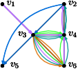
Figure 1: Example network for MD-SPP and MD-RSPP. The left-most image shows an input graph $D$. Five commodities for MD-SPP, $(v_{1},v_{2},\allowbreak(v_{1},v_{3},v_{6},v_{4},v_{2})),(v_{2},v_{5},(v_{2},v_{3},v_{5})),(v_{3},v_{2},(v_{3},v_{4},v_{2})),(v_{3},v_{4},(v_{3},v_{4})),(v_{3},v_{6},(v_{3},v_{6}))$, are represented in the second image. The third image gives a minimum target $(T=2)$ solution $H$ to the resulting MD-SPP instance. The last image illustrates that for MD-RSPP, by not fixing the paths of commodities, solutions $H$ with smaller target might exist (here $T=1$). Note that the multi-edges are only for illustration. A solution graph $H$ is in fact simple.

While both MD-SPP and MD-RSPP could be rather easily shown to be -complete on general graphs, Van Dyk, Klause, Koenemann and Megow showed that the former problem remains -complete even when restricted to orientations of stars [11]. In the rest of their article, they then focused on obtaining approximation as well as exact algorithms for MD-SPP on special classes of oriented trees. Apart from these individual results, the computational complexity of MD-RSPP and MD-SPP remains entirely unexplored.

Contributions. The central mission of this article is to provide a (near-)comprehensive parameterized analysis of the complexity of MD-RSPP and MD-SPP, with the aim of identifying precise conditions under which the problems become tractable. Our analysis will, in fact, reveal that the complexity-theoretic behavior of these problems is surprising and sometimes very different from the complexity of classical routing problems such as Vertex Disjoint Paths. Towards achieving our goal, we consider three natural types of parameterizations for the considered problems: parameterizing by the target solution quality (i.e., $T$), by the number of commodities, or by the structural properties of the input graph. The article is accordingly split into three parts, one for each of these perspectives.

In the first part of our article—Section 3—we establish that MD-SPP remains -hard already when $T=2$. Turning to MD-RSPP, we show that here -hardness holds already for the case of $T=1$. While the proofs of these results are non-trivial and work even on highly restricted inputs, this section is the least technically challenging of the three.

In Section 4, we turn towards an analysis of the considered problems when parameterized by the number of commodities. For both problems, we begin by establishing fixed-parameter tractability for the case of $T=1$ via a direct and stand-alone algorithm, as our more involved arguments for the general cases do not seemlessly transfer to this simpler setting. For MD-SPP, we then obtain a fixed-parameter algorithm for the general case by a kernelization argument that combines two main ingredients: a non-trivial data reduction rule that allows us to reduce the size of each “well-behaved” intersection of paths, and a Ramsey-type argument which guarantees that—after some simple preprocessing—every sufficiently large instance will contain some “well-behaved” intersection of paths. We note that the proof of this result is already more challenging than those required in Section 3, and the situation becomes even more difficult when we turn to MD-RSPP.

In order to solve MD-RSPP when $T\geq 2$, we first develop a preprocessing procedure which reduces the input into an equivalent one such that the length of every directed path is upper-bounded by a function of the parameter. This result can, on its own, already serve as the main ingredient of an  algorithm for MD-RSPP on general graphs. It is perhaps worth noting that—in spite of some superficial similarity between the problems—the -tractability of MD-RSPP contrasts the known para-hardness of Vertex Disjoint Paths (parameterized by the number of paths) on directed graphs [14, 26].

While it remains open whether the aforementioned -tractability can be improved to a fixed-parameter algorithm for MD-RSPP on general graphs w.r.t. the number of commodities, we conclude the section by showing that the problem is fixed-parameter tractable when the input digraph is planar. The proof of this result employs a further preprocessing procedure which does not result in a problem kernel, but instead obtains a graph of bounded radius. Even though bounded-radius planar graphs are known to have bounded treewidth [31, 30], we still cannot use this to solve the problem directly by, e.g., applying Courcelle’s Theorem [5] since the transitive closure need not have bounded treewidth. We complete the proof by branching to determine a bounded-size “template” which characterizes the structure of the sought-after solution, and then using Courcelle’s Theorem to check whether this template can be realized in the instance.

In Section 5, we target graph-structural parameterizations which would allow us to solve MD-SPP and MD-RSPP for arbitrary choices of $T$ and arbitrarily many commodities. Given the previously established -hardness of MD-SPP on orientations of stars—and the fact that the same reduction also works for MD-RSPP—one could ask whether parameterizing by treewidth plus the maximum vertex degree (of the underlying undirected graph) suffices; after all, this combined parameterization has already been successfully employed to achieve fixed-parameter algorithms for a number of other challenging problems, including, e.g., Edge Disjoint Paths [18]. Unfortunately, our reductions in Section 3 already establish the -hardness of both problems of interest even on bounded-degree trees.

As our final contribution, we show that the intractability of both problems can be overcome if one takes the maximum length of any admissible route as a third parameter. In particular, we devise a fixed-parameter algorithm that relies on dynamic programming to solve both MD-SPP and MD-RSPP when parameterized by the treewidth and maximum degree of the input graph (or, more precisely, its underlying undirected graph) plus the maximum length of a route in a solution. We complement this result with lower bounds which prove that all three of these parameters are necessary: dropping any of the three results in -hardness for both problems.

A summary of our complexity results for the two problems is provided in Table 1.

Parameter	Variant	Complexity	Reference
Target $T$	both	-hard for $T\geq 2$	Thm. 3.2
	MD-RSPP	-hard for $T\geq 1$	Thm. 3.4
Number $|K|$ of Commodities	both	FPT for $T\leq 1$	Thm. 4.1
	MD-SPP	FPT	Thm. 4.5
	MD-RSPP	FPT on planar graphs	Thm. 4.13
	MD-RSPP	XP	Thm. 4.11
Structural	both	FPT par. by degree + treewidth + path length	Thm. 5.1
		para-hard par. by degree + treewidth	Thm. 3.2
		para-hard par. by treewidth + path length	[11] & Fact 3
		para-hard par. by degree + path length	Thm. 5.3 & 5.5

Table 1: Complexity results for MD-SPP and MD-RSPP by different parameterizations. The parameters degree and treewidth refer to the underlying undirected graph of the input graph $D$. The parameter path length refers to the maximum length of any path fulfilling a commodity.

2 Preliminaries

For $k\in\mathbb{N}$, we denote by $[k]$ the set ${\{1,\dots,k\}}$.

Graph Terminology.  We employ standard graph-theoretic terminology [9]. For a directed graph $D=(V,E)$, let $\Delta_{D}^{+}(v)$ and $\Delta_{D}^{-}(v)$ be the sets of out-neighbors and in-neighbors of $v$, respectively, for all $v\in V$. Let $\delta_{D}^{+}(v)=|\Delta_{D}^{+}(v)|$, $\delta_{D}^{-}(v)=|\Delta_{D}^{-}(v)|$, $\delta^{+}(D)=\max_{v\in V}\delta_{D}^{+}(v)$, and $\delta^{-}(D)=\max_{v\in V}\delta_{D}^{-}(v)$. We may omit the subscript where $D$ is clear from context. For $u,v\in V$, a path in $D$ from $u$ to $v$ is called a $u$-$v$-path. For two graphs $D,D^{\prime}$, we say that $D^{\prime}$ is a subgraph of $D$ and write $D^{\prime}\subseteq D$ if $V(D^{\prime})\subseteq V(D^{\prime})$ and $E(D^{\prime})\subseteq E(D)$. The induced subgraph $D[X]$ of a vertex set $X\subseteq V(D)$ is defined by $V(D[X])=X$ and $E(D[X])=(X\times X)\cap E(D)$. The transitive closure of $D$, denoted by ${\cal T}(D)$, is the directed graph on the vertex set $V(D)$, whereas an edge $(i,j)$ exists in ${\cal T}(D)$ if and only if there is a directed path from $i$ to $j$ in $D$.

Let $G$ be a connected undirected graph. For two vertices of $v$ and $v^{\prime}$, denote by $\text{dist}(v,v^{\prime})$ the length of a shortest path from $v$ to $v^{\prime}$ in $G$. The eccentricity of a vertex $v$ in $G$ is defined as $\max_{v^{\prime}\in V(G)}{\{\text{dist}(v,v^{\prime})\}}$, and the radius of $G$ is the minimum eccentricity over all vertices of $G$. The underlying undirected graph of a directed graph $D$, denoted by $\mathcal{G}(D)$, is the undirected simple graph obtained from $D$ by replacing each directed edge with an undirected one.

Parameterized Complexity.  In parameterized complexity [10, 6], the complexity of a problem is studied not only with respect to the input size, but also with respect to some problem parameter(s). The core idea behind parameterized complexity is that the combinatorial explosion resulting from the -hardness of a problem can sometimes be confined to certain structural parameters that are small in practical settings. Formal definitions are provided below.

A parameterized problem $Q$ is a subset of $\Omega^{*}\times\mathbb{N}$, where $\Omega$ is a fixed alphabet. Each instance of $Q$ is a pair $(I,\kappa)$, where $\kappa\in\mathbb{N}$ is called the parameter. A parameterized problem $Q$ is fixed-parameter tractable (FPT) if there is an algorithm, called a fixed-parameter algorithm, that decides whether an input $(I,\kappa)$ is a member of $Q$ in time $f(\kappa)\cdot|I|^{\mathcal{O}(1)}$, where $f$ is a computable function and $|I|$ is the input instance size. The class FPT denotes the class of all fixed-parameter tractable parameterized problems.

Some of our algorithmic results rely on the exhaustive application of reduction rules, which are simple procedures that transform one input into another (typically smaller) input of the same problem. A reduction rule is safe if it preserves YES- and NO-instances, i.e., applying it on a YES- (NO-) instance results in a YES- (NO-) instance.

The class XP contains parameterized problems that can be solved in time ${\mathcal{O}\!\left(|I|^{f(\kappa)}\right)}$, where $f$ is a computable function. We say that a parameterized problem is para-hard if it remains -hard even when restricted to instances with a fixed value of the parameter.

Treewidth.  A nice tree decomposition $T$ of a graph $G=(V,E)$ is a pair $(T,\chi)$, where $T$ is a tree (whose vertices are called nodes) rooted at a node $t_{r}$ and $\chi$ is a function that assigns each node $t$ a set $\chi(t)\subseteq V$ such that the following hold:

• For every $uv\in E$, there is a node $t$ such that $u,v\in\chi(t)$.

• For every vertex $v\in V$, the set of nodes $t$ satisfying $v\in\chi(t)$ forms a subtree of $T$.

• $|\chi(\ell)|=0$ for every leaf $\ell$ of $T$ and $|\chi(t_{r})|=0$,

• There are only three kinds of non-leaf nodes in $T$:

  • introduce node: a node $t$ with exactly one child $t^{\prime}$ such that $\chi(t)=\chi(t^{\prime})\cup{\{v\}}$ for some vertex $v\notin\chi(t^{\prime})$.

  • forget node: a node $t$ with exactly one child $t^{\prime}$ such that $\chi(t)=\chi(t^{\prime})\setminus{\{v\}}$ for some vertex $v\in\chi(t^{\prime})$.

  • join node: a node $t$ with two children $t_{1},t_{2}$ such that $\chi(t)=\chi(t_{1})=\chi(t_{2})$.

We call each set $\chi(t)$ a bag, and we use $c(t)$ to denote the set of all vertices of $G$ which occur in the bag of some descendant of $t$ (possibly $\chi(t)$ itself). The width of a nice tree decomposition $(T,\chi)$ is the size of the largest bag $\chi(t)$ minus 1, and the treewidth of $G$ is the minimum width of a nice tree decomposition of $G$.

Courcelle’s Theorem.  One of the ingredients in the proof of Theorem 4.13 is Courcelle’s Theorem, which we introduce in this paragraph. We consider Monadic Second Order (MSO₂) logic on (edge-)labeled directed graphs in terms of their incidence structure, where the universe contains vertices and edges and the incidence between vertices and edges is represented by a binary relation. We assume an infinite supply of individual variables $x,x_{1},x_{2},\dots$ and of set variables $X,X_{1},X_{2},\dots$. The atomic formulas are $Vx$ (“$x$ is a vertex”), $Ey$ (“$y$ is an edge”), $Ixy$ (“vertex $x$ is incident with edge $y$”), $x=y$ (equality), $P_{a}x$ (“vertex or edge $x$ has label $a$”), and $Xx$ (“vertex or edge $x$ is an element of set $X$”). Formulas in MSO₂ logic are built from atomic formulas using the usual Boolean connectives $(\lnot,\land,\lor,\rightarrow,\leftrightarrow)$, quantification over individual variables ($\forall x$, $\exists x$), and quantification over set variables ($\forall X$, $\exists X$).

The free and bound variables of a formula are defined in the usual way. To indicate that the set of free individual variables of formula $\Phi$ is $\{x_{1},\dots,x_{\ell}\}$ and the set of free set variables of formula $\Phi$ is $\{X_{1},\dots,X_{q}\}$ we write $\Phi(x_{1},\ldots,x_{\ell},X_{1},\dots,X_{q})$. If $G$ is a digraph, $v_{1},\ldots,v_{\ell}\in V(G)\cup E(G)$ and $S_{1},\dots,S_{q}\subseteq V(G)\cup E(G)$ we write $G\models\Phi(v_{1},\ldots,v_{\ell},S_{1},\dots,S_{q})$ to denote that $\Phi$ holds in $G$ if the variables $x_{i}$ are interpreted by the vertices or edges $v_{i}$, for $i\in[\ell]$, and the variables $X_{i}$ are interpreted by the sets $S_{i}$, for $i\in[q]$.

The following result (the well-known Courcelle’s Theorem [5]) shows that if $G$ has bounded treewidth then we can find an assignment $\varphi$ to the set of free variables $\mathcal{F}$ with $G\models\Phi(\varphi(\mathcal{F}))$ (if one exists) in linear time.

Fact A (Courcelle’s Theorem [5, 1]).

Let $\Phi(x_{1},\dots,x_{\ell},X_{1},\dots,X_{q})$ be an MSO₂ formula with free individual variables $x_{1},\dots,x_{\ell}$ and free set variables $X_{1},\dots,X_{\ell}$, and let $w$ be an integer. Then there is an algorithm $\mathcal{A}$ that:

• takes as input an $n$-vertex labeled directed graph $G$ of treewidth at most $w$,

• either outputs $v_{1},\ldots,v_{\ell}\in V(G)\cup E(G)$ and $S_{1},\dots,S_{q}\subseteq V(G)\cup E(G)$ such that $G\models\Phi(v_{1},\ldots,v_{\ell},S_{1},\dots,S_{q})$ or correctly identifies that no such vertices $v_{1},\ldots,v_{\ell}$ and sets $S_{1},\dots,S_{q}$ exist, and

• runs in time $f(w,|\Phi(x_{1},\dots,x_{\ell},X_{1},\dots,X_{q})|)\cdot n$ for some computable function $f$.

Problem-Specific Definitions.  For a routed commodity $(s,t,P)$ in an MD-SPP instance or a commodity $(s,t)$ in an MD-RSPP instance, we call $s$ its source and $t$ its destination. For an MD-SPP instance $(D,K,T)$ and $v\in V(D)$, we let $P(v)=\{(s,t,P)\mid(s,t,P)\in K,\allowbreak P$ contains $v\}$ be the set of routed commodities with paths using $v$. For an MD-RSPP instance $(D^{\prime},K^{\prime},T^{\prime})$ and $v\in V(D^{\prime})$, we overload the same notation $P(v)=\{(s,t)\mid(s,t)\in K,\allowbreak D^{\prime}$ contains a directed $s$-$t$-path that passes through $v\}$ to denote the set of commodities which could be routed via $v$. We assume w.l.o.g. that each target is reachable from its corresponding source in the input MD-RSPP instance (as otherwise the instance can be rejected). A graph $H$ satisfying the conditions given in the problem statements is called a solution graph.

We provide a simple observation on trivial YES-instances of the two problems. If the target is at least the maximum outdegree of the input graph, then we are guaranteed to have a YES-instance since the input graph can be trivially used as the output graph. The same also holds if the target is at least the maximum number of commodities starting at any vertex, as then there is a solution by only using the edges $(s,t)$ for all commodities $(s,t)$ or $(s,t,P)$.

All instances of MD-SPP and MD-RSPP where the target is at least the maximum outdegree of the input graph or the maximum number of commodities starting at the same vertex are YES-instances.

3 Complexity Classification from the Perspective of the Target

Our first—and in a sense introductory—technical section is dedicated to the study of MD-SPP and MD-RSPP when parameterized by the value of the target $T$. We begin by noting that both problems of interest are trivially solvable in linear time if $T=0$. Further, we show that these problems are para-hard when parameterized by $T$.

To show this, we reduce from the strongly -hard 3-Partition problem [19].

Problem 3.1.

In particular, 3-Partition remains strongly -hard if all integers $n_{1},\ldots,n_{3m}$ are distinct [21].

Theorem 3.2.

MD-SPP and MD-RSPP are -hard, even when restricted to instances where $T\leq 2$ and $\mathcal{G}(D)$ is a tree of maximum degree at most $4$.

Proof 3.3.

We give a reduction from 3-Partition with distinct positive integers to MD-RSPP. The same construction holds for MD-SPP as well by assigning each commodity its unique path in the constructed graph.

We construct $D$ as follows. Let there be a path of $2mB+2m$ vertices. Let $S$ be the set of the first $2m$ vertices with labels $s_{1},s^{\prime}_{1},\ldots,s_{m},s^{\prime}_{m}$ (in the order they appear in the path). The next $mB$ vertices form the set $W$ and are indexed by the numbers $n_{1},\ldots,n_{3m}$, specifically $w_{1}^{1},\ldots,w_{1}^{n_{1}},\ldots,w_{3m}^{1},\ldots,w_{3m}^{n_{3m}}$. Among the remaining $mB$ vertices, which form the set $R$, there are $B$ vertices for each triple to be created, that is, $r_{1}^{1},\ldots,r_{1}^{B},\ldots,r_{m}^{1},\ldots,r_{m}^{B}$. For all $i\in[m]$, create the commodities $(s_{i},s^{\prime}_{i})$ and ${\{(s_{i},r_{i}^{j})\mid j\in[B]\}}$. For all $i\in[3m]$, create the commodities ${\{(w_{i}^{j},w_{i}^{j+1})\mid j\in[n_{i}-1]\}}$. For all $i\in[3m]$, create a vertex $\tilde{w}_{i}$, and add the edge $(w_{i}^{n_{i}},\tilde{w}_{i})$ and a commodity $(w_{i}^{n_{i}},\tilde{w}_{i})$. For all $i\in[m]$ and $j\in[B]$, create vertices $\tilde{r}_{i}^{j}$ and $\bar{r}_{i}^{j}$, and add the two edges and two commodities $(r_{i}^{j},\tilde{r}_{i}^{j})$ and $(r_{i}^{j},\bar{r}_{i}^{j})$. The resulting graph $D$ is depicted in Figure 2.

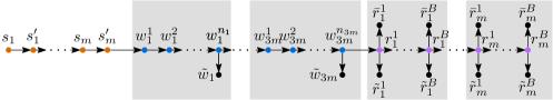
Figure 2: Constructed graph $D$ for the proof of Theorem 3.2. Vertices in $S$ are colored orange, those in $W$ are blue and those in $R$ are violet.

Then the 3-Partition instance is a YES-instance if and only if there is a solution to MD-RSPP in $D$ with target 2. Intuitively, for each $i\in[m]$ there are three available edges from $s_{i}$ and $s^{\prime}_{i}$ that can be used to select three subpaths in the middle section, representing three integers. Each subpath $w_{j}^{1},\ldots,w_{j}^{n_{j}}$ allows for $n_{j}$ outgoing edges, thus the subpaths have to be chosen such that their sum is at least $B$ to satisfy the commodities from $s_{i}$ to the last part of the path.

Formally, suppose the 3-Partition instance is a YES-instance. For all $i\in[m]$, let the $i^{\text{th}}$ triple in the solution be $(n_{\star(i,1)},n_{\star(i,2)},n_{\star(i,3)})$. We define

$$E_{S} :={\{(s_{i},s^{\prime}_{i})\mid i\in[m]\}},$$

$$E_{R} :={\{(r_{i}^{j},\tilde{r}_{i}^{j}),(r_{i}^{j},\bar{r}_{i}^{j})\mid i\in[m],j\in[B]\}}.$$

For all $$i\in[3m]$$ we define

$$E_{W}^{i} :={\{(w_{i}^{j},w_{i}^{j+1})\mid j\in[n_{i}-1]\}}\cup{\{(w_{i}^{n_{i}},\tilde{w}_{i})\}},$$

and for all $$i\in[m]$$ we define

$$E_{C}^{i} :={\{(s_{i},w_{\star(i,1)}^{1}),(s^{\prime}_{i},w_{\star(i,2)}^{1}),(s^{\prime}_{i},w_{\star(i,3)}^{1})\}},$$

$$E_{R}^{i} :={\{(w_{\star(i,1)}^{j},r_{i}^{j})\mid j\in[n_{\star(i,1)}]\}}\cup{\{(w_{\star(i,2)}^{j},r_{i}^{j+n_{\star(i,1)}})\mid j\in[n_{\star(i,2)}]\}}$$

$$\hphantom{=\{}\cup{\{(w_{\star(i,3)}^{j},r_{i}^{j+n_{\star(i,1)}+n_{\star(i,2)}})\mid j\in[n_{\star(i,3)}]\}}.$$

Finally,

$$E_{H} :=E_{S}\cup E_{R}\cup\bigcup_{i\in[3m]}E_{W}^{i}\cup\bigcup_{i\in[m]}E_{C}^{i}\cup\bigcup_{i\in[m]}E_{R}^{i}.$$

Consider the graph $H$ with edges $E_{H}$. Then $\delta^{+}(H)=2$ as in fact $\delta^{+}(v)=2$ for each of the $2mB+2m$ vertices $v$ along the main path and $\delta^{+}(v)=0$ for all other vertices. Observe that $E_{R}$ and all $E_{W}^{i}$ satisfy all commodities starting in vertices of $R$ and $W$, respectively, and $E_{S}$ satisfies all commodities with both endpoints in $S$. The remaining commodities start at the vertices $s_{1},\ldots,s_{m}$ and each lead to a set of $B$ vertices in $R$, such that the sets are pairwise disjoint. For $i\in[m]$, note that $s_{i}$, by also using $s^{\prime}_{i}$, is connected to the first vertex of three subpaths of vertices in $W$, that the total length of these subpaths is exactly $B$, and that each of the vertices in the subpaths connects to a distinct destination required for $s_{i}$. Thus, these remaining commodities are satisfied as well, and $H$ is a solution to the MD-RSPP instance.

Now suppose there is a solution $H$ to the MD-RSPP instance with target 2. First note that for all $i\in[3m]$ we have $E_{S},E_{R},E_{W}^{i}\subseteq E(H)$, as otherwise there would be unsatisfied commodities. By $E_{R}\subseteq E(H)$ alone, we have that each vertex in $R$ has outdegree 2, and they can have no other edges in $E(H)$. As each $t\in R$ is the destination of one commodity, this implies that there have to be $|R|=mB$ individual edges from $V\setminus R$ to $R$ in $E(H)$. By construction of $D$, these edges have to start in $S$ or $W$ as otherwise they would not be in ${\cal T}(D)$. Each of the $mB+2m$ vertices in $S\cup W$ is allowed 2 out-edges, out of which $E_{S}$ and the $E_{W}^{i}$ already use $mB+m$. This leaves another $mB+3m$ edges, out of which $mB$ have to go to $R$. We will show below that the remaining $3m$ edges have to end in the first vertex in each of the $3m$ subpaths in $W$, that is, in each of $w_{1}^{1},\ldots,w_{3m}^{1}$. In total, the entire available outdegree of $S$ and $W$ is accounted for.

Suppose one of the $3m$ edges would not connect to a subpath. This would save 1 edge that can be connected to $R$, but now there is $j\in[3m]$ such that there is no connection from $S$ to any $w_{j}^{1},\ldots,w_{j}^{n_{j}}$. As $n_{j}$ of the edges in our calculation start in $w_{j}^{1},\ldots,w_{j}^{n_{j}}$ and can then not be used for fulfilling commodities, this would reduce the total number of available edges by $n_{j}-1$. As $n_{j}>\frac{B}{4}$ and we can assume $B\geq 4$ (otherwise the 3-Partition instance becomes trivial), this reduces the amount of available edges by at least 1 and there are no longer enough edges to satisfy all commodities ending in $R$. The same issue arises when connecting to some vertex $w_{i}^{j}$ instead of $w_{i}^{1}$ for some $i\in[3m],j>1$. Hence, the remaining $3m$ edges end in the vertices $w_{1}^{1},\ldots,w_{3m}^{1}$. In particular, this implies that there are no $a,b\in[m],a\neq b$ such that $s_{a}$ and $s_{b}$ are connected to the same subpath $w_{j}^{1},\ldots,w_{j}^{n_{j}}$ in $H$.

We now argue that $s_{i}$ is connected to exactly three subpaths $w_{j}^{1},\ldots,w_{j}^{n_{j}}$ in $H$ and that the total length of these subpaths is $B$. We then have a solution to 3-Partition where the $i^{\text{th}}$ triple is $n_{a},n_{b},n_{c}$ where $s_{i}$ is (not necessarily directly) connected to $w_{a}^{1},w_{b}^{1},$ and $w_{c}^{1}$. Note that we just established that these triples are pairwise disjoint as no two vertices $s_{a},s_{b},a\neq b$ connect to the same subpath. Consider any $i\in[m]$ and the remaining three outgoing edges of $s_{i}$ and $s^{\prime}_{i}$. As argued above, they either end in $R$ or distinct vertices in $W_{1}={\{w_{1}^{1},\ldots,w_{3m}^{1}\}}$. If $s_{i}$ is connected to no subpath, the three edges cannot cover all commodities of $s_{i}$. Thus, there is $a\in[3m]$ such that $(s_{i},w_{a}^{1})$ or $(s^{\prime}_{i},w_{a}^{1})$ is in $E(H)$. As this used one edge and $w_{a}^{1},\ldots,w_{a}^{n_{a}}$ has $n_{a}$ outgoing edges, we now have $n_{a}+2$ edges available. As we still assume $B\geq 4$ and have $n_{a}<\frac{B}{2}$, this does not suffice. Thus, there is $b\in[3m]$ such that one of the $n_{a}+2$ available edges ends in $w_{b}^{1}$. Now, there are $n_{a}+n_{b}+1$ edges available. However, recall that $n_{a}\neq n_{b}$, so we have $n_{a}+n_{b}-1<\frac{B}{2}+\frac{B}{2}-1+1=B$, so these edges still do not suffice. Thus, there is $c\in[3m]$ such that one of the $n_{a}+n_{b}+1$ available edges ends in $w_{c}^{1}$. This gives $n_{a}+n_{b}+n_{c}$ edges available for connecting to $r_{i}^{1},\ldots,r_{i}^{B}$. As for all $i\in m$ we have that $s_{i}$ is connected to at least 3 distinct vertices in $W_{1}$ and $|W_{1}|=3m$ we have that there is no $s_{i}$ that is connected to more than 3 vertices in $W_{1}$. Hence, each $s_{i}$ is associated with a triple $n_{a},n_{b},n_{c}$, has exactly $n_{a}+n_{b}+n_{c}$ edges available to connect to its $B$ distinct destinations in $R$. Thus, for each $s_{i}$ we have $n_{a}+n_{b}+n_{c}\geq B$, and as $\sum_{j\in[3m]}n_{j}=mB$ we have $n_{a}+n_{b}+n_{c}=B$, yielding a solution to the 3-Partition instance.

For MD-RSPP, we can even show hardness for $T\leq 1$ by a straightforward reduction from Hamiltonian Cycle.

Theorem 3.4.

MD-RSPP is -hard when restricted to instances where $T\leq 1$.

Proof 3.5.

We reduce from Hamiltonian Cycle. Let $G$ be an undirected $n$-vertex graph and $D$ be the directed graph that is obtained by replacing every edge ${\{u,v\}}\in E(G)$ by two edges $(u,v)$ and $(v,u)$. Let $K={\{(u,v)\mid u,v\in V(G),u\neq v\}}$. Then $(D,K,1)$ is a YES-instance of MD-RSPP if and only if $G$ has a Hamiltonian cycle.

Indeed, suppose $G$ has a Hamiltonian cycle $(v_{1},v_{2},\dots,v_{n-1},v_{n})$. Let $H$ be such that $E(H)={\{(v_{1},v_{2}),\ldots,(v_{n-1},v_{n}),(v_{n},v_{1})\}}$. Then $\delta^{+}(H)=1$, $H\subseteq{\cal T}(D)$, and for each pair of vertices $u,v\in V$ there is a directed $u$-$v$-path in $H$. On the other hand, suppose there is a solution graph $H$ for $(D,K,1)$. As each vertex is both a source and a destination, it has at least one incoming and one outgoing edge in $H$. As $\delta^{+}(H)\leq 1$, this implies that $H$ is a cycle cover of $V$. Finally, as there is a commodity between each pair of vertices, $V$ has to be a connected component in $H$, and so $E(H)$ must be a Hamiltonian cycle.

4 Parameterizing by the Number of Commodities

This section is dedicated to the study of the considered parcel sortation problems when parameterized by the number of commodities. This line of enquiry can be seen as analogous to the fundamental questions that have been investigated for other prominent examples of problems typical for logistical networks, such as the study of Vertex and Edge Disjoint Paths parameterized by the number of paths or of Coordinated Motion Planning parameterized by the number of robots. We remark that the former has been shown to be fixed-parameter tractable in Robertson and Seymour’s seminal work [32], while the fixed-parameter tractability of the latter has only been established on planar grid graphs in a recent work of Eiben, Ganian and Kanj [12].

We first provide a straightforward proof that instances of both MD-SPP and MD-RSPP with target $T\leq 1$ are in FPT by the number of commodities (Theorem 4.1). This allows us to concentrate on the case of $T\geq 2$ in the rest of the section.

Theorem 4.1.

MD-SPP and MD-RSPP restricted to instances such that $T\leq 1$ are in FPT when parameterized by the number of commodities.

Proof 4.2.

We prove the statement by showing that there is an $f(|K|)$-kernel. Let ${\cal I}=(D,K,1)$ be an instance. Create a reduced instance ${\cal I}^{\prime}=(D^{\prime},K,1)$ as follows. Let $V(D^{\prime})$ contain only the vertices in $D$ that are the sources and destinations of the commodities in $K$. Then, for all $u,v\in V(D^{\prime})$, let $(u,v)\in E(D^{\prime})$ if and only if $(u,v)\in{\cal T}(D)$. Clearly, this reduction is computable in polynomial time and leaves a graph with at most $2|K|$ vertices. By brute forcing the reduced instance, this kernel can then be used to obtain FPT runtime. As ${\cal T}(D^{\prime})$ is a subgraph of ${\cal T}(D)$, any solution to ${\cal I}^{\prime}$ is a solution to ${\cal I}$. We conclude the proof by showing that if ${\cal I}$ is a YES-instance then it has a solution that does not use any of the deleted vertices by an exchange argument. Let $H$ be any solution to ${\cal I}$ and let $v$ be a non-source, non-destination vertex in $H$. If $v$ has no out-neighbor in $H$, it does not contribute to the solution and can be removed. Otherwise, as $H$ is a solution graph with outdegree 1, $v$ has a unique out-neighbor $w$ in $H$. Create a new solution $H^{\prime}$ by letting $V(H^{\prime})=V(H)\setminus{\{v\}}$, deleting the edge $(v,w)$, and replacing each edge $(u,v)\in E(H)$ by an edge $(u,w)\in E(H^{\prime})$. Then the outdegree of each vertex in $H^{\prime}$ is at most as large as its outdegree in $H$ and thus at most 1. Further, the connectivity between pairs of source or destination vertices did not change. Moreover, for MD-SPP for every commodity routed along an $s$-$t$-path $P$ there is still an $s$-$t$-path in $H^{\prime}\cap{\cal T}(P)$. In either case, $H^{\prime}$ is still a solution. By repeatedly applying this procedure, we can create a solution $H^{\prime}$ in which all non-source, non-destination vertices are removed.

4.1 A Fixed-Parameter Algorithm for MD-SPP

In this subsection, we establish the fixed-parameter tractability of MD-SPP under the aforementioned parameterization. Our proof relies on two main ingredients, the first of which is the generalized Ramsey’s Theorem:

Fact 1 ([29]).

There exists a function Ram: $\mathbb{N}\times\mathbb{N}\to\mathbb{N}$ with the following property. For each pair of integers $r,s$ and each clique $G$ of size at least Ram$(r,s)$ such that each edge has a single label (color) out of a set of $r$ possible labels, it holds that $H$ must contain a subclique $H$ of size at least s such that every edge in $H$ has the same label.

In particular, we remark that Ram has a computable upper bound. Secondly, we use the following reduction rule.

Reduction Rule $R_{1}$.  For an MD-SPP instance ${\cal I}=(D,K,T)$ with $T\geq 2$, let $U\subseteq K$, and $q={\left\lceil\frac{|U|}{T-1}\right\rceil}$. Suppose that there are vertices $v_{1},\dots,v_{2q+2}$ of $D$ such that $P(v_{1})=\dots=P(v_{2q+2})=U$, and for all commodities $(s,t,P)\in U$, the directed path $P$ visits these vertices in the order of either $(v_{1},\dots,v_{2q+2})$ or $(v_{2q+2},\dots,v_{1})$. Then we contract the vertices $v_{q+1}$ and $v_{q+2}$ into a vertex $c$ and remove the outgoing edges from $c$ to vertices other than $v_{1},\dots,v_{q},v_{q+3},\dots,v_{2q+2}$. $\diamond$

To avoid any confusion, we explicitly remark that the vertices $v_{1},\dots,v_{2q+2}$ need not be visited consecutively by the paths in $U$. An illustration of a concrete application of Reduction Rule $R_{1}$ is provided in Figure 3 later.

Lemma 4.3.

Reduction Rule $R_{1}$ is safe.

Proof 4.4.

Let ${\cal I}^{\prime}=(D^{\prime},K^{\prime},T)$ be the reduced instance. By assumption, $v_{1},\dots,v_{2q+2}$ are only used for the paths in $U$, and these paths visit these vertices in the order $v_{1},\dots,v_{2q+2}$ (right commodities) or $v_{2q+2},\dots,v_{1}$ (left commodities). Therefore, none of these vertices except for $v_{1}$ or $v_{2q+2}$ can be a source or a destination in $K$ or $K^{\prime}$.

Suppose there is a solution graph $H^{\prime}$ for ${\cal I}^{\prime}$ (in particular, this implies that $H^{\prime}$ is a subgraph of ${\cal T}(D^{\prime})$). We create a subgraph $H$ of ${\cal T}(D)$ from $H^{\prime}$ as follows. First, we set $V(H)=(V(H^{\prime})\setminus\{c\})\cup\{v_{q+1},v_{q+2}\}$. For the edge set, we also begin by keeping all edges not incident to $c$ in $E(H)$. For all $(v,c)\in E(H^{\prime})$, if $(v,v_{q+1})\in{\cal T}(D)$, let $(v,v_{q+1})\in E(H)$. Otherwise, we have $(v,v_{q+2})\in{\cal T}(D)$ and let $(v,v_{q+2})\in E(H)$. For all $(c,v)\in E(H^{\prime})$, let $(v_{q+1},v)\in E(H)$ and $(v_{q+2},v)\in E(H)$. Note that the outdegree of $c$ in $H^{\prime}$ and thereby the outdegree of $v_{q+1}$ and $v_{q+2}$ in $H$ is at most $T$. Further, there is no other vertex for which the outdegree increases, as every edge to $c$ was replaced with exactly one edge to either $v_{q+1}$ or $v_{q+2}$. Since the connectivity between all pairs of vertices (except $c,v_{q+1},$ and $v_{q+2}$) is the same in $H$ and $H^{\prime}$, $H$ is a solution to the original instance.

Now suppose there is a solution to ${\cal I}$ by some subgraph $H$ of ${\cal T}(D)$. We define $a\colon U\rightarrow[2q+2]$, where for each right (or left) commodity $u=(s,t,P)\in U$ we let $a(u)$ be the smallest (or largest) integer such that $s$ is connected to $v_{a(u)}$ in $H\cap{\cal T}(P)$. Create a subgraph $H^{\prime}$ of ${\cal T}(D^{\prime})$ as follows. Delete the vertices $v_{q+1}$ and $v_{q+2}$ with all incident edges from $H$ and add the vertex $c$. For all $v\in V$, if $(v,v_{q+1})$ or $(v,v_{q+2})$ in $H$, we add $(v,c)$ to $H^{\prime}$. Replace all edges $(v_{i},v_{j})$ where $i<j$ and $i\leq q$ or $i>j$ and $i\geq q+3$ by the edge $(v_{i},c)$. Now, for each right commodity $u$ which is no longer satisfied in $H^{\prime}$, we have $a(u)\leq q+2$; similarly, for each left commodity $u$ which is no longer satisfied in $H^{\prime}$, we have $a(u)\geq q+1$. In both cases, the starting vertex of the commodity is connected to $c$ in $H^{\prime}$. To account for these commodities, we independently modify the outgoing edges of the vertices $v_{1},\ldots,v_{q+1}$ and $v_{q+2},\ldots,v_{2q+2}$. We only describe the procedure to modify the edges from $v_{q+2},\ldots,v_{2q+2}$, as the modification of the vertices $v_{1},\ldots,v_{q+1}$ follows in a symmetrical fashion. The goal of this procedure is to change the out-edges of $v_{q+2},\ldots,v_{2q+2}$ to satisfy all right commodities by connecting $c$ to all targets of “unsatisfied” right commodities. While doing so, we have to ensure no satisfied right commodity becomes unsatisfied and all left commodities $u$ such that $a(u)>q+2$ are still connected to $c$. Intuitively, the procedure allows us to gradually route up to $T-1$ (or $T-2$) commodities directly to their destination and pass the remaining ones to the next vertex to the right.

Formally, for $b,j\in[2q+2],b\leq j$, let $U(b,j)$ be the set of commodities $u$ with $b\leq a(u)\leq j$. If there are no unsatisfied right commodities, we are done. Otherwise, let there be $w>0$ unsatisfied right commodities. Identify the smallest $j\in\mathbb{N}$ such that $j>q+2$ and $w\leq(T-1)\cdot(j-(q+2))-|U(q+3,j)|$. Then, iterate through $i=b+1,\ldots,j$. Each time, add the edge $(v_{i-1},v_{i})$ (or $(c,v_{i})$ if $i=q+3$) and delete all outgoing edges from $v_{i}$. (Note that as we delete these outgoing edges, some satisfied right commodities may become unsatisfied and some left commodities $u$ may no longer be able to reach $c$.) If there is at least one left commodity $u$ such that $a(u)=i$, add the edge $(v_{i},c)$ and choose $T-2$ unsatisfied right commodities; if there are less, choose all. Otherwise, choose (up to) $T-1$ unsatisfied right commodities. Then, add an edge $(v_{i},t)$ for the destination $t$ of each chosen commodity. Stop the procedure as soon as there are no unsatisfied right commodities left.

Example 1.

Suppose we have an MD-SPP instance $(D,K,T)$, where $T=2$, $q=3$ and we consider three routed commodities with source and destination $s_{i},t_{i}$, $i\in[3]$. Further, suppose we have a solution graph $H$ which contains a sequence $(v_{1},\dots,v_{8})$ of vertices satisfying the requirements of Reduction Rule $R_{1}$, as depicted in Figure 3(left), where the vertices $v_{q+1}$, $v_{q+2}$ are marked in orange. Figure 3 (middle) shows the intermediate graph $H^{\prime}$ with unsatisfied commodities after $v_{q+1}$ and $v_{q+2}$ are replaced by $c$. There, for $v_{q+1},v_{q+2}$, out-edges (such as $(v_{4},v_{1}),(v_{5},t_{2})$) are deleted and in-edges (such as $(sv_{6},v_{5})$) are replaced by edges to $c$. Edges starting before $v_{q+1}$ going right (like $(v_{2},v_{3}),(v_{3},v_{6})$) and edges starting after $v_{q+2}$ going left are replaced by edges to $c$. Figure 3 (right) shows the solution graph $H^{\prime}$ after the application of the symmetrical procedures which resolve all of the three unsatisfied commodities. There is one unsatisfied right commodity and two commodities $u$ such that $a(u)=6$. Thus the smallest $j$ guaranteeing enough outdegree in the vertices $v_{6},\ldots,v_{j}$ is $j=8$. Hence, the edge $(c,v_{6})$ is added and the out-edges of $v_{6}$ are deleted, but as there is a left commodity $u$ with $a(u)=6$, the edge $(v_{6},c)$ is added back in. The right commodity is still unsatisfied so the edge $(v_{6},v_{7})$ is added back in and the edge $(v_{7},t_{1})$ is used to satisfy the commodity. Note that in this case (due to the left edge resolving 2 commodities at once), we break the loop before reaching $v_{8}$. The symmetrical procedure applied to the left hand vertices works in a similar manner, but here each vertex resolves a distinct commodity ($v_{1}$ and $v_{3}$ satisfy the left commodities and $v_{2}$ connects $s_{1}$ to $c$.)

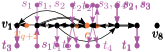
Figure 3: Illustrations for Example 1.

Consider the graph $H^{\prime}$ after the above procedure. Note that all added edges start in the sequence $(v_{1},\dots,v_{2q+2})$ and either end in the sequence or the destination of a commodity. Thus, $H^{\prime}$ remains a subgraph of ${\cal T}(D^{\prime})$. Further, by construction, no vertex has outdegree larger than $T$ in $H^{\prime}$, and if the procedure terminates successfully, $H^{\prime}$ satisfies all commodities in $U$. As all edges in $E(H^{\prime})\setminus E(H)$ have at least one endpoint in a vertex $v$ such that $P(v)=U$, the commodities outside $U$ remain unaffected by the changes.

Next, we argue that the procedure is guaranteed to terminate successfully. To this end, we show that (1) during the procedure if there is an unsatisfied right commodity, then there is $j$, such that $q+2<j\leq 2q+2$ and $w\leq(T-1)\cdot(j-(q+2))-|U(q+3,j)|$; (2) after the procedure, for any left commodity $u$ with $a(u)>q+2$, there is a path in $H^{\prime}$ from $a(u)$ to $c$; and (3) after the procedure, there is no unsatisfied right commodity $u$ left. For (1), let $j=2q+2$. As for all $w$ unsatisfied commodities $u$, we have $a(u)\leq q+2$, and hence, $w+|U(q+3,j)|\leq|U|$. By definition of $q$, we have $|U|\leq(T-1)q=(T-1)(2q+2-(q+2))$. The statement of (1) then follows. To see (2), note that such a left commodity is immediately resolved by the added edge $(v_{i},c)$. For (3), for a commodity $u=(s,t,P)$, if $a(u)>j$, then the directed path in ${\cal T}(P)\cap H$ is still present in $H^{\prime}$, as its vertices have not been changed. Thus, we only consider $u$ such that $a(u)\leq j$. Note that after connecting each vertex of $c,v_{q+3},\ldots,v_{j-1}$ to its successor, there are $(T-1)\cdot(j-(q+2))$ available outgoing edges in the vertices $v_{q+3},\ldots,v_{j}$. Thus, there is one edge for each of the at most $w+|U(q+3,j)|\leq(T-1)\cdot(j-(q+2))$ commodities to resolve. (To resolve a commodity $u$ means either to create a directed path from $a(u)$ to $c$ if $u$ is a left commodity or to create a directed path from $a(u)$ to the destination of $u$ if $u$ is a right commodity.) It remains to show that at the beginning of iteration $i$, if there is still an unsatisfied right commodity, then we have resolved $(T-1)$ commodities at each vertex $v_{j^{\prime}}$ for $q+2<j^{\prime}<i$. As $j$ is the minimum index such that $w+|U(q+3,j)|<(T-1)\cdot(j-(q+2))$, for all $q+2<j^{\prime}<j$ we have $w+|U(q+3,j^{\prime})|>(T-1)\cdot(j^{\prime}-(q+2))$, and hence the vertices $v_{q+3},\ldots,v_{j-1}$ can indeed resolve $(T-1)$ commodities each. As left commodities are immediately taken care of, the only remaining commodities are right commodities which can then be satisfied by $v_{j}$. In summary, the procedure successfully terminates. As the same holds true for the symmetrical procedure, $H^{\prime}$ is a solution to $I^{\prime}$.

We remark that carefully selecting a suitable interval for the symmetrical procedures is necessary and one cannot simply route commodities in a “greedy fashion” along the whole sequence. Intuitively, this is because a hypothetical solution may route the commodities in a way where they only enter the sequence at specific vertices; for instance, it may happen that many right commodities enter the sequence near its right endpoint.

Example 2.

Suppose we have a solution $H$ to the original instance resolving four right commodities in the two rightmost vertices, as depicted in Figure 4. Assume the target is $T=2$. Though by assumption the starting vertices have to be somehow connected to the other vertices in the sequence in the underlying graph $D$, commodities outside the sequence might enforce that the depicted connections to the sequence are the only available ones in any solution graph. Thus, the two rightmost vertices have to resolve these four commodities in both the original and the reduced instance. In the standard rerouting, where each vertex on the sequence is connected to its successor, these two vertices only have a total of three available outdegree left and cannot satisfy all four commodities. Thus, the algorithm is designed to leave these vertices unchanged and use the other vertices in the sequence to resolve all other commodities.

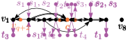
Figure 4: Example for the necessity of choosing a small interval to reorganize the resolution of commodities.

We now have all the components required to establish the main result of this subsection.

Theorem 4.5.

MD-SPP is in FPT parameterized by the number of (routed) commodities.

Proof 4.6.

Let $(D,K,T)$ be an MD-SPP with $|K|=k$. When $T\leq 1$, we have fixed-parameter tractability by Theorem 4.1. Therefore, we now assume that $T\geq 2$. Recall the Ram function from 1. Let $\overline{\textup{{Ram}}}:\mathbb{N}\times N\rightarrow N$ be a computable upper bound of Ram.

For any vertex $v$ such that $P(v)=\emptyset$, we can remove it and its incident edges from $D$, because no solution will use $v$. For any nonempty subset $U$ of $K$, let $q=\lceil|U|/(T-1)\rceil$. Let $V_{U}$ be the set of vertices $v$ such that $P(v)=U$. Let $(s_{1},t_{1},P_{1}),\dots,(s_{|U|},t_{|U|},P_{|U|})$ be the commodities in $U$. Define an edge-labeled complete graph on $V_{U}$, where the label of each edge is a $(|U|-1)$-tuple, whose $i^{\text{th}}$ element is a binary number to indicate whether $P_{i+1}$ visits the incident vertices of the edge in the same or opposite order as $P_{1}$. (Note that when $|U|=1$, there is only one label.) As long as $|V_{U}|\geq\overline{\textup{{Ram}}}(2^{|U|-1},2q+2)$, we choose an arbitrary subset of $V_{U}$ of size $\overline{\textup{{Ram}}}(2^{|U|-1},2q+2)$, and by 1, we can find a subclique of size $2q+2$ whose edges have the same label. In other words, the paths in $U$ visit the vertices in this subclique either in the same order as $P_{1}$ does or in the reversed order. Then we can apply Reduction Rule $R_{1}$ to reduce the size of $V_{U}$ by one. Repeating this procedure, we obtain an instance where

$$|V_{U}|<\overline{\textup{{Ram}}}(2^{k-1},2k+2).$$

After processing all subsets $U$ of $K$, we obtain an instance whose input graph has at most $2^{k}\cdot\overline{\textup{{Ram}}}(2^{k}-1,2k+2)$ vertices. By Section 2, we can assume $T$ is at most the maximum outdegree of the input graph. Therefore, the resulting instance has size bounded by a function of $k$ and can be brute-forced in FPT time.

Since the reduction rule reduces the number of vertices by one, and since we apply the reduction rule after every application of 1, in total, we apply 1 and the reduction rule at most $|V(D)|$ times. An application of the reduction rule takes ${\mathcal{O}\!\left(|V(D)|\right)}$ time. To find the subclique guaranteed by 1, we can use a brute force approach of trying all $(2q+2)$-vertex subset of the vertex set of size $\overline{\textup{{Ram}}}(2^{|U|-1},2q+2)$. This takes time ${\mathcal{O}\!\left(\overline{\textup{{Ram}}}(2^{k-1},2k+2)^{(2k+2)}\right)}$. In total, the run time is ${\mathcal{O}\!\left(|V(D)|^{2}+|V(D)|g(k)\right)}$ for some computable function $g$.

4.2 Parameterized Algorithms for MD-RSPP

We start by obtaining a reduction rule to eliminate all long paths in the input graph that is similar in spirit to the one used for MD-SPP, but works for unrouted commodities (Lemmas 4.7 and 4.9). This then yields an XP algorithm by the number of commodities (Theorem 4.11). In the second half of the subsection, we show that MD-RSPP is also fixed-parameter tractable under the same parameterization when restricted to planar input graphs; this is achieved via a combination of nontrivial branching, a structural result on bounded-radius planar graphs and Courcelle’s Theorem (Theorem 4.13).

Reduction Rule and -tractability. We define our reduction rule for MD-RSPP below.

Reduction Rule $R_{2}$.  For an MD-RSPP instance ${\cal I}=(D,K,T)$ with $T\geq 2$, let $U\subseteq K$, and $q={\left\lceil\frac{|U|}{T-1}\right\rceil}$. Suppose that there is a directed path $(v_{1},\dots,v_{q+1})$ in ${\cal T}(D)$ such that $P(v_{1})=\dots=P(v_{q+1})=U$ and $v_{1}$ is neither a source nor a destination for any commodity. Then we remove $v_{1}$ and its incident edges from $D$, and for every removed edge $(v,v_{1})$, we add an edge $(v,v^{\prime})$, where $v^{\prime}$ is an out-neighbor of $v_{1}$ and either $v^{\prime}=v_{2}$ or $v^{\prime}$ is on a directed path from $v_{1}$ to $v_{2}$. $\diamond$

We note that in Reduction Rule $R_{2}$, the edge $(v,v^{\prime})$ is added instead of $(v,v_{2})$ in order to preserve the planarity of the underlying graph $D$. This will be useful for obtaining Theorem 4.13 later on.

Lemma 4.7.

Reduction Rule $R_{2}$ is safe.

Proof 4.8.

It is easy to see that every solution to the reduced instance is a solution to the original instance.

Suppose there is a solution to the original instance ${\cal I}$ by some subgraph $H$ of ${\cal T}(D)$. We now construct a solution to the reduced instance $(D^{\prime},K,T)$. The idea for this construction follows closely the proof of Lemma 4.3. We define $a\colon U\to[q+1]$, where for each commodity $u=(s,t)\in U$ we let $a(u)$ be minimal such that there is a directed path from $s$ to $t$ via $v_{a(u)}$ in $H$. We assume that $a(u)$ exists for every commodity $u$ in $U$; otherwise, we remove $u$ from $U$. Create a subgraph $H^{\prime}$ of ${\cal T}(D^{\prime})$ as follows. Remove the vertex $v_{1}$ and its incident edges from $H$, and for every removed edge $(v,v_{1})$, add the edge $(v,v_{2})$. (Note that the reduction rule guarantees that $(w,v_{2})$ is still an edge in ${\cal T}(D)$.) Because of these operations, some commodities may become unsatisfied. For $b,j\in[q+1],b\leq j$, let $U(b,j)$ be the set of commodities $u$ with $b\leq a(u)\leq j$. If there are no unsatisfied commodities, we are done. Otherwise, let $w>0$ be the number of unsatisfied commodities. Identify the smallest $j\in\mathbb{N}$ such that $j>1$ and $w\leq(T-1)\cdot(j-1)-|U(2,j)|$. Then, iterate through $i=2,\ldots,j$. Each time, add an edge $(v_{i-1},v_{i})$ if $i>2$, and delete all outgoing edges from $v_{i}$. (Note that as we delete these outgoing edges, more commodities may become unsatisfied.) Choose $T-1$ unsatisfied commodities. Then, add an edge $(v_{i},t)$ for the destination $t$ of each chosen commodity. Break the loop as soon as there are no unsatisfied commodities left.

Consider the graph $H^{\prime}$ after the above procedure. Note that all added edges start in the path $(v_{2},\dots,v_{q+1})$ and either end at a later vertex in the path or the destination of a commodity. Thus, $H^{\prime}$ remains a subgraph of ${\cal T}(D^{\prime})$. Further, by construction, no vertex has outdegree larger than $T$ in $H^{\prime}$, and if the procedure terminates successfully, $H^{\prime}$ satisfies all commodities in $U$. As all edges in $E(H^{\prime})\setminus E(H)$ have at least one endpoint in a vertex $v$ such that $P(v)=U$, the commodities outside $U$ remain unaffected by the changes.

What remains to be shown is that the procedure terminates successfully. To this end, we can use similar arguments as in the proof of Lemma 4.3 to show that (1) during the procedure, if there is an unsatisfied commodity, then there is $j$, such that $1<j\leq q+1$ and $w\leq(T-1)\cdot(j-1)$; and (2) after the procedure, there no unsatisfied commodity left.

Crucially, the exhaustive application of Reduction Rule $R_{2}$ allows us to bound the length of all directed paths in $D$:

Lemma 4.9.

Every MD-RSPP instance $(D,K,T)$ such that $T\geq 2$ can be reduced to an equivalent instance $(D^{\prime},K,T)$ such that all directed paths in $D^{\prime}$ have length at most $2|K|^{2}$ in $f(|K|)|V(D)|^{\mathcal{O}(1)}$ time. Further, for every YES-instance there is a solution graph $H$ that is the union of paths $P_{1},\ldots,P_{|K|}$, where each $P_{i}$ connects the source of the $i^{\text{th}}$ commodity to its destination and has length at most $2|K|^{2}$.

Proof 4.10.

Let $|K|=k$. For each vertex $v$ such that $P(v)=\emptyset$, we can remove it and its incident edges from $D$, since no solution will use $v$. As long as there is a directed path $Q=v_{1},\ldots,v_{\ell}$ such that $\ell>2k^{2}$, proceed as follows. Partition $Q$ into subsequences $S_{1},\ldots,S_{d}$ such that we have $P(v)=P(v^{\prime})$ for all vertices $v,v^{\prime}\in S_{i}$, $i\in[d]$. Note that the vertices of each subsequence $S_{i}$ form a path in the transitive closure, so by exhaustively applying Reduction Rule $R_{2}$ we obtain an equivalent instance where each subsequence $S_{i}$ contains at most ${\left\lceil\frac{k}{T-1}\right\rceil}\leq k$ non-source, non-destination vertices. Observe that for $i,j\in[\ell],i<j$ and some commodity $u\in K$, if $P(v_{i})$ and $P(v_{j})$ both contain $u$, then $P(v_{i^{\prime}})$ also contains $u$ for $i\leq i^{\prime}\leq j$. Thus, along the sequence $(P(v_{1}),\ldots,P(v_{\ell}))$, each commodity is only added and removed once, giving $d\leq 2k-2$. Thus, along the path $P=v_{1},\ldots,v_{\ell}$, each commodity is only added and removed once, giving $d\leq 2k-2$ as there are at most that many subsequences with vertices $v$ with non-empty $P(v)$. Hence, after exhaustively applying the above procedure, each directed path has length at most $(2k-2)k+2k=2k^{2}$ by also considering the at most $2k$ source or destination vertices. Identifying a path of length $2k^{2}$ or showing that none exists takes $\mathcal{O}\!\left((2k^{2})!\cdot|V(D)|\cdot|E(D)|\right)$ time using Monien’s algorithm [27]. This time dominates the time to then apply Reduction Rule $R_{2}$. This is repeated less than $V(D)$ times as each application removes a vertex. Thus, the exhaustive reduction procedure takes time in $\mathcal{O}\!\left(k!\cdot|V(D)|^{3}\right)$.

For the second statement, note that there are only $k$ commodities, and for each of them, all paths connecting its source and destination have length at most $2k^{2}$. Consider any solution graph $H$ and choose any $s$-$t$-path for each of the $k$ commodities $(s,t)$. Delete all vertices (including their incident edges) that are not represented in any chosen path. The modified graph $H$ is still a solution graph.

Lemma 4.9 allows us to derive a direct  algorithm for the problem.

Theorem 4.11.

MD-RSPP is in  parameterized by the number of commodities.

Proof 4.12.

Let ${\cal I}=(D,K,T)$ be an MD-RSPP instance. If $T\leq 1$, solve the instance using Theorem 4.1. Otherwise, by Lemma 4.9, there is a solution using at most $2|K|^{3}$ vertices. There are at most $\sum_{i=1}^{2|K|^{3}}\binom{|V(D)|}{i}$ choices of these vertices and for each choice there are less than $2^{(4|K|^{6})}$ ways to connect them. For each setting, we can test in time $f(k)$ for some computable function $f$ whether it is a valid solution.

The Planar Case.  Unfortunately, we are not able to resolve the question of whether MD-RSPP is fixed-parameter tractable on general graphs using the tools outlined above. In particular, while Lemma 4.9 intuitively allows us to view the problem as a special case of either (Induced) Subgraph Detection or Minor Detection, the former class of problems are [1]-hard on directed and undirected graphs while the latter remains elusive (and difficult to formalize) on directed graphs. Nevertheless, in this subsection we show that MD-RSPP is indeed fixed-parameter tractable at least when restricted to planar digraphs.

For the proof of this result, it will be useful to recall Courcelle’s Theorem (A) and the following relationship between treewidth and the radius of planar graphs.

Fact 2 ([30]).

A planar graph $G$ with radius at most $r$ has treewidth at most $3r+1$.

It is worth noting that 2 does not allow us to bound the treewidth of the transitive closure ${\cal T}(D)$ of $D$; indeed, even if $\mathcal{G}(D)$ is a star, ${\cal T}(D)$ may easily contain large complete (bipartite) graphs. While this prevents a direct application of Courcelle’s Theorem on $D$ to solve the problem, in the following proof we show that this difficulty can be overcome by carefully branching to determine a bounded-size “template” of the solution.

Theorem 4.13.

MD-RSPP on planar input digraphs $D$ is in FPT when parameterized by the number of commodities.

Proof 4.14.

Let $(D,K,T)$ be an MD-RSPP instance. If $T\leq 1$, by Theorem 4.1, there is a fixed-parameter algorithm to decide the instance. Hence, we can assume that $T\geq 2$. Let $k:=|K|$ and let $u_{1},\dots,u_{k}$ be the commodities in $K$. We first apply Lemma 4.9 to obtain an instance $(D,K,T)$ where every directed path has length at most $2k^{2}$.

In order to find a solution graph in FPT-time, we first bound the treewidth of $\mathcal{G}(D)$. We assume $\mathcal{G}(D)$ to be connected, because otherwise, we can apply our algorithm on each connected component of $\mathcal{G}(D)$ independently. We show that the radius of $\mathcal{G}(D)$ is at most $4k^{3}$. Observe that for two vertices $v$ and $v^{\prime}$ of $\mathcal{G}(D)$ and some commodity $(s,t)\in K$, if $(s,t)\in P(v)\cap P(v^{\prime})$, then there are directed paths from $v$ and $v^{\prime}$ to $t$ in $D$; combining these two paths yields an undirected path between $v$ and $v^{\prime}$ of length at most $4k^{2}$ in $\mathcal{G}(D)$. Now for two arbitrary vertices $v,v^{\prime}$, since $\mathcal{G}(D)$ is connected, there is a path $Q$ from one vertex to the other in $\mathcal{G}(D)$. By the above observation, we can modify $Q$ such that it is still a $v$-$v^{\prime}$-path but for each commodity $u\in|K|$ and the subpath between the first vertex and last vertex among the vertices $v_{u}$ for which $u\in P(v_{u})$, this subpath has length at most $4k^{2}$. Thus, the length of $Q$ is at most $4k^{3}$, given that we deleted all vertices $v_{0}$ for which $P(v_{0})=\emptyset$. Thereby, the radius of $\mathcal{G}(D)$ is at most $4k^{3}$. It is easy to see that Reduction Rule $R_{2}$ preserves planarity. By 2, we conclude that the treewidth of $\mathcal{G}(D)$ is at most $12k^{3}+1$.

Lemma 4.9 further gives that there is a solution represented by the union over $k$ paths connecting the commodities in $H$. Each $s$-$t$-path in $H$ has an underlying $s$-$t$-path in $D$ and this path has length at most $2k^{2}$. We thus fix the start and destination vertices of the commodities and branch on all $f(k)$ possible unions $D^{\prime}$ of $s_{i}$-$t_{i}$-paths in $D$, for $i\in[k]$. For each of these possibilities, we branch on the $f^{\prime}(k)$ possible subgraphs of their transitive closure, disregarding those that are invalid solutions by not satisfying some commodity or exceeding the target outdegree. It remains to decide whether any of the created graphs $D^{\prime}$ is an isomorphic subgraph of $D$. Let $V(D^{\prime})={\{w_{1},\ldots,w_{q}\}}$, $q\in{\mathcal{O}\!\left(k^{3}\right)}$. Given that $\mathcal{G}(D)$ has bounded treewidth, we can decide whether $D^{\prime}$ is an isomorphic subgraph of $H$ with respect to the fixed source and target vertices by employing Courcelle’s Theorem (A) with the following $\text{MSO}_{2}$-formula of length $\mathcal{O}\!\left(q^{2}\right)$:

$$\varphi(D)=\exists_{v_{1},\ldots,v_{q}\in V(D)}\colon\forall_{i,j\in[q],i\neq j}\colon v_{i}\neq v_{j}\wedge\text{preserveEdge}(v_{i},v_{j})\wedge\text{preserveType}(v_{i}).$$

Here, preserveEdge$(v_{i},v_{j})$ is TRUE if and only if $(w_{i},w_{j})\notin E(D^{\prime})$ or $(v_{i},v_{j})$ in $D$. Further, preserveType$(v_{i})$ is TRUE if and only if $v_{i}$ is the source/destination of the $j^{\text{th}}$ commodity if and only if $w_{i}$ is the source/destination of the $j^{\text{th}}$ commodity.

5 Structural Parameters

In our final section, we turn towards a graph-structural analysis of the considered parcel sortation problems. We note that at first glance, it may seem difficult to identify a “reasonable” graph-structural parameter that could be used to solve MD-SPP or MD-RSPP: the -hardness of both problems on an orientation of a star ([11] in combination with 3) rules out not only the use of treewidth (as by far the most widely used structural graph parameter), but also a range of other much more restrictive parameterizations such as treedepth [28], the vertex cover number [7, 35, 3] and various directed variants of treewidth [15, 16].

The above situation is not unique: there is a well-known example of another routing problem—Edge Disjoint Paths—which suffers from a similar difficulty, notably by being para-hard even on undirected graphs with vertex cover number $3$ [13]. But for Edge Disjoint Paths, one can achieve fixed-parameter tractability when parameterizing by the combination of treewidth and the maximum degree [18], while for MD-SPP and MD-RSPP we can exclude tractability even under this combined parameterization by recalling Theorem 3.2.

The above considerations raise the question: Are there any structural restrictions under which we can efficiently solve instances of MD-SPP or MD-RSPP involving a large number of commodities and target? As the main contribution of this section, we answer this question positively by identifying the maximum route length as the missing ingredient required for tractability. Indeed, from an application perspective, restricting one’s attention only to physical routes which do not involve too many intermediary nodes is well-aligned with practical considerations for the routing of most goods. From a formal perspective, for the purposes of this section we will assume that the parameterized instances of MD-SPP and MD-RSPP come equipped with an additional integer parameter $p$ called path length and:

• for MD-SPP, it holds that the path $P$ of every routed commodity has length at most $p$;

• for MD-RSPP, we require that for every commodity $(s,t)\in K$, there exists a directed $s$-$t$-path $P^{\prime}$ in $H$ with a corresponding base path $P$ in $D$ (formally, $P^{\prime}\subseteq{\cal T}(P)$) such that $P$ has length at most $p$. To formally distinguish it from MD-RSPP, we denote this enriched problem by MD-RSPP_PL, and note that for $p\geq|V(G)|$ the problems coincide.

As our first result, we establish the fixed-parameter tractability of both problems of interest when $p$ is included in the parameterization.

Theorem 5.1.

MD-SPP and MD-RSPP_PL are in FPT by the combination of the treewidth and maximum degree of $\mathcal{G}(D)$ and the path length.

Proof 5.2.

Let $(D,K,T)$ be an MD-RSPP_PL or MD-SPP instance with path length $p$. Let $tw$ and $\delta_{\max}$ be the treewidth and maximum degree of $\mathcal{G}(D)$, respectively.

Consider a nice tree decomposition $(\mathtt{T},X)$ of $\mathcal{G}(D)$ with treewidth at most $tw$. We use the standard dynamic programming technique that starts at the leaves of the decomposition and traverses up to the root. For each node $b$ of $\mathtt{T}$, let $N(b)$ denote the set of all vertices that are in $X(b)$ or have distance at most $p$ in $\mathcal{G}(D)$ to a vertex in $X(b)$. We define a state with respect to a node $b$ as a pair $(d,R)$ of a function $d:N(b)\to{\{0,\dots,T\}}$ and a directed graph $R$ over the vertices in $N(b)$ with $\delta^{+}(R)\leq T$. We say that a state $(d,R)$ is a candidate if there is a graph $H_{d}^{R}$ such that

1. $H_{d}^{R}\subseteq{\cal T}(D[c(b)\cup N(b)])$;

2. Every vertex has outdegree at most $T$ in $H_{d}^{R}$;

3. For MD-RSPP_PL, for every commodity $(s,t)\in K$ such that $s\in c(b)$ or $t\in c(b)$, there is a directed $s$-$t$-path in $H_{d}^{R}$ with a base path of length at most $p$ in $D$ and for MD-SPP, for every commodity $(s,t,P)\in K$ such that $s\in c(b)$ or $t\in c(b)$, there is a directed $s$-$t$-path in $H_{d}^{R}\cap{\cal T}(P)$;

4. $R=H_{d}^{R}[N(b)]$;

5. Every vertex $v\in N(b)$ has outdegree $d(v)$ in $H_{d}^{R}$.

Clearly, if the the root $r$ has a candidate $(d,R)$, then $H_{d}^{R}$ is a solution to the $(D,K,T)$ instance. Further, if the instance $(D,K,T)$ is solved by some $H\subseteq{\cal T}(D)$, the root has a candidate $(d,R)$, where $d$ assigns each vertex in $N(b)$ its outdegree in $H$ and $R=H[N(b)]$. Thus, identifying whether the root has a candidate suffices to decide the instance. We use the following dynamic program to identify all candidates at each node of $\mathtt{T}$.

At every node, we create a table that indicates whether a state $(d,R)$ of the node is a candidate, defined recursively as follows.

• For a leaf, the only candidate is $(d,R)$, where $d$ is an empty function and $R$ the graph with $V(R)=\emptyset$.

• For an introduce node $\bar{b}$ that introduces a vertex $v$ into a bag $X(b)$, a state $(\bar{d},\bar{R})$ of $\bar{b}$ is a candidate if there exists a candidate $(d,R)$ of $b$, such that

  • $\bar{R}\subseteq{\cal T}(D[N(\bar{b})])$;

  • $E(\bar{R})\cap(N(b)\times N(b))=E(R)$;

  • For every $u\in N(b)$, we have $\bar{d}(u)=d(u)+|{\{(u,w)\in E(\bar{R})\mid w\in N(\bar{b})\setminus N(b)\}}|\leq T$;

  • For every $u\in N(\bar{b})\setminus N(b)$, we have $\bar{d}(u)\leq T$ and $\bar{d}(u)=\delta^{+}_{\bar{R}}(u)$;

  • For MD-RSPP_PL, for every $(s,v)\in K$ (or $(v,s)\in K)$ there is a directed $s$-$v$-path ($v$-$s$-path) in $\bar{R}$ with a base path in $D$ of length at most $p$, and for MD-SPP, for every $(s,v,P)\in K$ (or $(v,s,P)\in K)$ there is a directed $s$-$v$-path ($v$-$s$-path) in $\bar{R}\cap{\cal T}(P)$.

• For a forget node $\bar{b}$ that removes a vertex $v$ from a bag $X(b)$, a state $(\bar{d},\bar{R})$ of $\bar{b}$ is a candidate, if there exists a candidate $(d,R)$ of $b$, such that $\bar{R}=R[N(\bar{b})]$ and for every $u\in N(\bar{b})$, $\bar{d}(u)=d(u)$.

• For a join node $\bar{b}$ that joins two nodes $b$ and $b^{\prime}$, a state $(\bar{d},R)$ of $\bar{b}$ is a candidate, if there exist candidates $(d,R)$ and $(d^{\prime},R)$ of $b$ and $b^{\prime}$, respectively, such that for all $v\in N(\bar{b})$, $\bar{d}(v)=d(v)+d^{\prime}(v)-\delta_{R}^{+}(v)$ and $\bar{d}(v)\leq T$.

We assume $\delta_{\max}>1$, because otherwise $D$ is a union of disjoint edges, so the problem can easily be solved in linear time. Then for each vertex $v$ of $D$, $N(v)$ is loosely bounded by $\delta_{\max}^{p+1}$. Consider any node $b$. We have $X(b)\leq tw+1$ and $N(b)\leq(tw+1)\delta_{\max}^{p+1}$. For every state of $b$, we have that $d$ takes one of $T+1$ possible values for every $v\in N(b)$ and there are at most $(\sum_{i=0}^{T+1}\binom{N(b)}{i})^{N(b)}$ possible graphs for $R$. Therefore, the number of states of $b$ is less than

$$(T+1)^{|N(b)|}\cdot\left(\sum_{i=0}^{T+1}\binom{N(b)}{i}\right)^{N(b)}<(\delta_{\max}+1)^{(tw+1)\delta_{\max}^{p+1}}\cdot\left(\sum_{i=0}^{\delta_{\max}+1}\binom{(tw+1)\delta_{\max}^{p+1}}{i}\right)^{(tw+1)\delta_{\max}^{p+1}}$$

where by Section 2, we assume that $T<\delta_{\max}$. Hence, the size of each table is bounded by some computable function $f(tw,\delta_{\max},p)$. Further, we note that by the above rules computing all candidates of each node in a dynamic programming manner from the leaves to the root takes FPT time.

We conclude the proof by noting that the above algorithm correctly identifies the candidates at each node as shown in the claim below.

The algorithm correctly identifies all candidates for each node. We prove by induction along the tree decomposition. For some directed graph $H$ and a set of vertices $S\subseteq V(H)$ we define the graph $H[S]_{{\cal T}}:=\big{(}S,\,E(H)\cap{\cal T}(D[S])\big{)}$; that is, it is the subgraph of $H$ on $S$ that only keeps edges in the transitive closure of $D[S]$.

Leaves.  Here, the only candidate is the empty function and the graph with no vertices.

Introduce Nodes.  Suppose node $\bar{b}$ introduces a vertex $v$ into a bag $X(b)$. Suppose the algorithm sets $(\bar{d},\bar{R})$ to be a candidate of $\bar{b}$ as witnessed by some $(d,R)$. By the induction hypothesis, $(d,R)$ is a candidate for $b$ witnessed by some graph $H_{d}^{R}$. We create a graph $H_{\bar{d}}^{\bar{R}}$ by combining $H_{d}^{R}$ and $\bar{R}$. In particular, $V(H_{\bar{d}}^{\bar{R}})=c(\bar{b})\cup N(\bar{b})\supseteq V(H_{d}^{R})$ and $E(H_{\bar{d}}^{\bar{R}})=E(H_{d}^{R})\cup E(\bar{R})$. Then (a) and (d) hold by construction and (b),(c), and (e) hold by combining the properties of $H_{d}^{R}$ with the five properties of $\bar{d}$ and $\bar{R}$ as defined in the algorithm’s introduce step.

For the other direction, let node $\bar{b}$ have a candidate $(\bar{d},\bar{R})$ witnessed by some $H_{\bar{d}}^{\bar{R}}$. Let $H_{d}^{R}=H_{\bar{d}}^{\bar{R}}[c(b)\cup N(b)]_{{\cal T}}$, $d(v)=\delta^{+}_{H_{d}^{R}}$ for every $v\in N(b)$, and $R=H_{d}^{R}[N(b)]$. Then $(d,R)$ is a candidate for node $b$ as witnessed by $H_{d}^{R}$, where (a), (d), and (e) hold by construction, while (b) and (c) hold due to the candidate properties of $H_{\bar{d}}^{\bar{R}}$. In particular, for (c), we remark that all paths starting or ending in $X(b)$ of length at most $p$ only use vertices in $N(b)$ and thereby do not use any of the removed edges. By induction, the algorithm identifies $(d,R)$ as a candidate for node $b$. What remains to be shown is that the algorithm identifies $(d,R)$ as a witness for $(\bar{d},\bar{R})$ being a candidate of $\bar{b}$. To see this, first note that $\bar{R}\subseteq{\cal T}(D[N(\bar{b})])$ as $(\bar{d},\bar{R})$ is a candidate. By construction, $E(\bar{R})\cap(N(b)\times N(b))=R$ and, as $v\in c(\bar{R})$, condition (c) for $(\bar{d},\bar{R})$ implies that all commodities starting or ending in $v$ are satisfied by $\bar{R}$. Further, (b) gives that $\bar{d}(u)\leq T$ for all $u\in N(\bar{b})$ and (e) gives for all $u\in N(\bar{b})\setminus N(b)$ that $\bar{d}(u)=\delta^{+}_{\bar{R}}(u)$ by noting that all neighbors of $u$ are in $\bar{R}$. Last, for vertices in $N(b)$, by construction we have that $\bar{d}$ equals $d$ with the additional outdegree with edges to or from $N(\bar{b})\setminus N(b)$.

Forget Nodes.  Suppose a node $\bar{b}$ removes a vertex $v$ from a bag $X(b)$. Suppose the algorithm sets $(\bar{d},\bar{R})$ to be a candidate of $\bar{b}$ as witnessed some $(d,R)$. By induction, $(d,R)$ is a candidate for $b$ with a respective graph $H_{d}^{R}$. Let $H_{\bar{d}}^{\bar{R}}=H_{d}^{R}$. Then (b)–(e) hold by construction and (a) follows by $N(b)\setminus N(\bar{b})\subseteq c(b)$, which holds as follows. Let $u\in N(b)\setminus N(\bar{b})$. Then there is a path of length at most $p$ from $u$ to $v$ that does not visit any vertices in $X(\bar{b})$. Let $(u^{\prime},v)$ be the last edge of this path. Thus, by the tree decomposition, $u^{\prime}$ and $v$ have to share some bag and as $v\notin X(\bar{b})$, we have $u^{\prime}\in c(b)$. By the same reasoning, as the path from $u$ to $u^{\prime}$ does not pass through $X(b)$, we have $u\in c(b)$.

For the other direction, let node $\bar{b}$ have a candidate $(\bar{d},\bar{R})$ witnessed by some $H_{\bar{d}}^{\bar{R}}$. Let $H_{d}^{R}=H_{\bar{d}}^{\bar{R}}$, for every $v\in N(b)$ let $d(v)=\delta_{H_{d}^{R}}^{+}(v)$, and $R=H_{d}^{R}[N(b)]$. Then $(d,R)$ is a candidate for node $b$ as witnessed by $H_{d}^{R}$, where (a) holds as $c(b)=c(\bar{b})$ and $N(\bar{b})\subseteq N(b)$, and $(b)$–$(e)$ hold by construction. By induction, the algorithm identifies $(d,R)$ as a candidate for node $b$. Further, as $\bar{R}=R[N(\bar{b})]$, the algorithm identifies $(\bar{d},\bar{R})$ as a candidate for node $\bar{b}$ as witnessed by $(d,R)$.

Join Nodes.  Suppose a node $\bar{b}$ joins two nodes $b$ and $b^{\prime}$. Suppose the algorithm sets $(\bar{d},R)$ to be a candidate of $\bar{b}$ as witnessed by some $(d,R)$ and $(d^{\prime},R)$ that are, by induction, candidates of $b$ and $b^{\prime}$, respectively. Let $H_{d}^{R}$ and $H_{d^{\prime}}^{R}$ be the graphs witnessing them as candidates, respectively. Define $H_{\bar{d}}^{R}$ as their union graph. Conditions (a), (c), and (d) follow immediately from the candidate properties of $H_{d}^{R}$ and $H_{d^{\prime}}^{R}$. For condition (b), let $v\in c(\bar{b})\cup N(\bar{b})$. Note that $H_{d}^{R},H_{d^{\prime}}^{R}$, and $H_{\bar{d}}^{R}$ share the induced subgraph $R$. As $H_{d}^{R}$ and $H_{d^{\prime}}^{R}$ fulfil (b), $\delta_{H_{\bar{d}}^{R}}^{+}(v)>T$ would imply that $\Delta_{H_{\bar{d}}^{R}}^{+}(v)\setminus N(\bar{b})\cap c(b)\neq\emptyset$ and $\Delta_{H_{\bar{d}}^{R}}^{+}(v)\setminus N(\bar{b})\cap c(b^{\prime})\neq\emptyset$. In particular, $v$ would have edges to both $c(b)\setminus X(\bar{b})$ and $c(b^{\prime})\setminus X(\bar{b})$. By the tree decomposition this implies $v\in X(\bar{b})$, which in turn gives that all its neighbors are in $N(\bar{b})$. Thus there can be no such $v$ and (b) holds. For condition (e), let $v\in N(\bar{b})$. Note that $\Delta_{H_{\bar{d}}^{\bar{R}}}(v)\subseteq V(H_{d}^{R})\cup V(H_{d^{\prime}}^{R})$, $|\Delta_{H_{\bar{d}}^{\bar{R}}}(v)\cap V(H_{d}^{R})|=d(v)$, and $|\Delta_{H_{\bar{d}}^{\bar{R}}}(v)\cap V(H_{d^{\prime}}^{R})|=d^{\prime}(v)$. Further, $\Delta_{H_{\bar{d}}^{\bar{R}}}(v)\cap V(H_{d}^{R})\cap V(H_{d^{\prime}}^{R})=\Delta_{R}^{+}(v)$, as $u\in c(b)$ and $u\in c(b^{\prime})$ imply $u\in X(\bar{b})$ by the tree decomposition. Hence, $|\Delta_{H_{\bar{d}}^{\bar{R}}}(v)|=d(v)+d^{\prime}(v)-\delta_{R}^{+}(v)$ and the algorithm correctly identifies $(\bar{d},R)$ as a candidate.

For the other direction, let node $\bar{b}$ have a candidate $(\bar{d},R)$ witnessed by some $H_{\bar{d}}^{R}$. Let $H_{d}^{R}=H_{\bar{d}}^{R}[c(b)\cup N(\bar{b})]_{{\cal T}}$ and $H_{d^{\prime}}^{R}=H_{\bar{d}}^{R}[c(b^{\prime})\cup N(\bar{b})]_{{\cal T}}$. Let $d$ and $d^{\prime}$ assign every vertex in $N(\bar{b})$ its outdegree in $H_{d}^{R}$ or $H_{d^{\prime}}^{R}$, respectively. Then $(d,R)$ and $(d^{\prime},R)$ are candidates for nodes $b$ and $b^{\prime}$, respectively, as witnessed by $H_{d}^{R}$ and $H_{d^{\prime}}^{R}$, where (a), (b), (d), and (e) hold by construction and (c) holds as every path of length at most $p$ that uses a vertex in $c(b)$ (or $c(b^{\prime})$) cannot use a vertex outside $c(b)\cup N(\bar{b})$ (or $c(b)\cup N(\bar{b})$) and no edge outside ${\cal T}(D[c(b)\cup N(\bar{b})])$ (or ${\cal T}(D[c(b)\cup N(\bar{b})])$). By induction, the algorithm correctly identifies $(d,R)$ and $(d^{\prime},R)$ as candidates. By the same reasoning as above we have $\bar{d}(v)=|E_{v}|=d(v)+d^{\prime}(v)-|{\{u\mid(v,u)\in E(R)\}}|$ for all $v\in N(\bar{b})$, so the algorithm correctly identifies $(\bar{d},R)$ as a candidate for node $\bar{b}$ with $(d,R)$ and $(d^{\prime},R)$ as witnesses.

Note that the constructions above can be used for a backtracking approach that allows us to reconstruct the graph $H_{d}^{R}$ for any candidate $(d,R)$. Thus, the dynamic program described in the proof of Theorem 5.1 can not only solve the decision problem but also output a solution $H$.

In the remainder of this section, we complement Theorem 5.1 by showing that if any of the three parameters (treewidth, degree, and path length) is not bounded, both problems become -hard. Theorem 3.2 in Section 3 already establishes this when dealing with instances of unbounded path length. Van Dyk, Klause, Koenemann, and Megow [11] proved MD-SPP to be -hard even when the input graph is a star where every leaf has either an in- or out-edge to the center but never both. As in such graphs, for each commodity there is a unique path connecting its source and destination, the same construction can be used for MD-RSPP_PL.

Fact 3 ([11]).

MD-RSPP_PL and MD-SPP with path length $p=2$ on stars are -hard.

Finally, we also establish -hardness even for bounded-degree digraphs where commodities have bounded path length. To this end, we reduce from the -complete 3-SAT-(2,2) problem, which is the restriction of 3-SAT to the case where each clause has exactly three literals and each literal occurs in exactly two clauses [8].

Theorem 5.3.

MD-RSPP_PL is -hard, even when restricted to instances where $T\leq 2$, the path length is at most $4$, and $\mathcal{G}(D)$ has maximum degree at most $7$.

Proof 5.4.

Suppose we have an instance of 3-SAT-(2,2) with a set $C$ of $m$ clauses and a set $X$ of $n$ variables. Construct $D$ as follows. For every variable $x\in X$, we use the variable gadget as in Figure 5 (left) and add the following commodities to $K$: $(s_{x},t)$ for $t\in{\{t_{x},t^{\prime}_{x},t^{\prime\prime}_{x}\}}$. For every clause $c\in C$ over the literals $x,y$, and $z$, we use the clause gadget as in Figure 5 (right). There, the vertices of $x,y$, and $z$ correspond to the respective literal vertex ($x$ or $\bar{x}$) in the variable gadgets. Further, we add the following commodities to $K$: $(c,t)$ for $t\in{\{x,y,z,t_{c}\}}$. Observe that literal vertices have the highest degree (3 in- and 4 out-edges) as they are part of one variable and two clause gadgets. The constructed MD-RSPP_PL instance with $p=4$ has a solution with target at most $2$ if and only if the 3-SAT-(2,2) instance is a YES-instance.

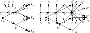
Figure 5: Variable gadget (left) and clause gadget (right) for the proof of Theorem 5.3. Orange colored vertices are shared between different gadgets.

Suppose we have a YES-instance of 3-SAT-(2,2). Consider the graph $H$ such that $V(H)=V(D)$ and

$$E(H) =\bigcup_{x\in X}E_{x}\cup\bigcup_{c\in C}E_{c},$$

$$E_{x} =\begin{cases}{\{(s_{x},\bar{x}),(s_{x},t_{x}),(\bar{x},t_{x}^{\prime}),(\bar{x},t_{x}^{\prime\prime})\}},\quad\text{if $x$ is TRUE;}\\ {\{(s_{x},x),(s_{x},t_{x}^{\prime\prime}),(x,t_{x}),(x,t_{x}^{\prime})\}},\quad\text{else;}\\ \end{cases}$$

$$E_{c} ={\{(c,c^{\prime}),(c,x),(c^{\prime},y),(c^{\prime},z),(a,t_{c})\}},$$

where $a\in{\{x,y,z\}}$ is any TRUE literal in the clause. Observe that $H$ is a subgraph of ${\cal T}(D)$ and for every commodity $(s,t)\in K$ there is a directed $s$-$t$-path in $H$. Further, the outdegree of vertices $s_{x},c$, $c^{\prime}$ for a variable $x$ or clause $c$ are 2 and the outdegrees of $t_{x},t_{x}^{\prime},t_{x}^{\prime\prime},t_{c}$ are 0. Each literal vertex ($x$ or $\bar{x}$) that is FALSE has 2 outdegree in its variable gadget and no outdegree towards a clause gadget vertex. Each literal vertex that is TRUE has no outdegree inside its variable gadget and at most outdegree 1 in each of the two clause gadgets it appears in. Thus, $H$ is a solution for target 2.

Now suppose there is a solution $H$ for the MD-RSPP instance with target 2. Consider the gadget of a variable $x$. To fulfil all commodities inside the gadget while preserving a maximum outdegree of 2 in $H$, we have ${\{(x,t_{x}),(x,t_{x}^{\prime})\}}\subseteq E(H)$ or ${\{(\bar{x},t_{x}^{\prime}),(\bar{x},t_{x}^{\prime\prime})\}}\subseteq E(H)$. We let $x$ be FALSE if the first holds and $x$ be TRUE if only the second holds. This variable assignment from all variable gadget satisfies all clauses as follows. Consider any clause $c$ over the literals $x,y,z$. To fulfil all commodities inside the gadget while preserving a maximum outdegree of 2 in $H$, we have ${\{(c,x),(c,c^{\prime}),(c^{\prime},y),(c^{\prime},z)\}}\subseteq E(H)$. Then, $c$ and $c^{\prime}$ cannot have an edge to $t_{c}$ in $E(H)$ without exceeding the target of 2. Thus, $(a,t_{c})\in E(H)$ for at least one $a\in{\{x,y,z\}}$. This literal has to be TRUE (and thereby satisfies the clause) because otherwise literal $a$ would have at least outdegree 3 in $H$ (two in its variable gadget and one in the clause gadget).

We modify the proof of Theorem 5.3 using more sophisticated gadgets to account for the fixed paths and obtain a similar result for MD-SPP.

Theorem 5.5.

MD-SPP is -hard, even when restricted to instances where $T\leq 4$, the path length is at most $5$ and $\mathcal{G}(D)$ has maximum degree at most $11$.

Proof 5.6.

Suppose we have an instance of 3-SAT-(2,2) with a set $C$ of $m$ clauses and a set $X$ of $n$ variables. Construct $D$ as follows. For every variable $x$, we use the variable gadget as in Figure 6 (left) and add the following commodities to $K$: $(s_{x},t)$ for $t\in{\{t^{x}_{1},t^{x}_{2},t^{x}_{3},t^{\bar{x}}_{1},t^{\bar{x}}_{2},t^{\bar{x}}_{3},t^{\bar{x}}_{4}\}}$. The directed paths for these commodities are exactly the unique directed paths in the gadget. For every clause $c$ over the literals $x,y$, and $z$, we use the clause gadget as in Figure 6 (right) and add the following commodities to $K$. First, add $(a,t)$ for $a\in{\{c,c^{\prime},c^{\prime\prime},\tilde{c}\}}$ and $t\in{\{t^{a}_{1},t^{a}_{2}\}}$. Second, add $(c,c^{\prime})$ and $(c^{\prime},c^{\prime\prime})$. All of these commodities are assigned their unique respective path. Last, add $(c,t)$ for $t\in{\{t^{c,a}_{1},t^{c,a}_{2}|a\in{\{x,y,z\}}\}}$. For $a\in{\{x,y,z\}}$, the directed path for $(c,t_{1}^{c,a})$ (or $(c,t_{2}^{c,a})$) is the unique directed path from $c$ to $t_{1}^{c,a}$ (or $t_{2}^{c,a}$) that contains $a$. Observe that vertices $\tilde{c}$ have the highest outdegree (3 in- and 8 out-edges).

Figure 6: Variable gadget (left) and clause gadget (right) for the proof of Theorem 5.5. Orange colored vertices are shared between different gadgets.

Suppose we have a YES-instance of 3-SAT-(2,2). Consider the graph $H$ such that

$$E(H) =\bigcup_{x\in X}E_{x}\cup\bigcup_{c\in C}E_{c},$$

$$E_{x} =\begin{cases}{\{(s_{x},\bar{x})\}}\cup{\{(s_{x},t_{i}^{x})\mid t\in[3]\}}\cup{\{(\bar{x},t_{i}^{\bar{x}})\mid t\in[4]\}},\hphantom{,(x,t_{4})}\quad\text{if $x$ is TRUE;}\\ {\{(s_{x},x),(x,t_{4}^{\bar{x}})\}}\cup{\{(x,t_{i}^{x})\mid t\in[3]\}}\cup{\{(s_{x},t_{i}^{\bar{x}})\mid t\in[3]\}},\quad\text{else.}\\ \end{cases}$$

$$E_{c} ={\{(a,t_{1}^{a}),(a,t_{2}^{a})\mid a\in{\{c,c^{\prime},c^{\prime\prime},\tilde{c}\}}\}}\cup{\{(c,c^{\prime}),(c^{\prime},c^{\prime\prime}),(c,\tilde{c}),(c^{\prime},x),(x,t_{1}^{c,x}),(x,t_{2}^{c,x})\}}$$

$$\hphantom{=}\cup{\{(c^{\prime\prime},t_{1}^{c,y}),(c^{\prime\prime},t_{2}^{c,y}),(\tilde{c},t_{1}^{c,z}),(\tilde{c},t_{2}^{c,z})\}},$$

where without loss of generality $x$ is a TRUE literal in the clause. Observe that $H$ is a subgraph of ${\cal T}(D)$ and for every commodity $(s,t,P)\in K$ there is a directed $s$-$t$-path in $H\cap{\cal T}(P)$. Further, the outdegree of vertices $t_{i}^{x}$ is 0 and the outdegree of vertices $s_{x},c,c^{\prime},c^{\prime\prime},$ and $\tilde{c}$ is 4. Each literal vertex ($x$ or $\bar{x}$) that is FALSE has 4 outdegree in $E_{x}$ and no outdegree in any $E_{c}$. Each literal vertex that is TRUE has no outdegree in $E_{x}$ and at most outdegree 2 in each of $E_{c}$, $E_{c^{\prime}}$, the two clause gadgets it appears in. Thus, $H$ is a solution for target 4.

Now suppose there is a solution $H$ for the MD-SPP instance with target 4. Consider the gadget of a variable $x$ and partition the vertices in two sets $S_{x}=(s_{x},x,\bar{x})$ and $T_{x}={\{t_{1}^{x},t_{2}^{x},t_{3}^{x},t_{1}^{\bar{x}},t_{2}^{\bar{x}},t_{3}^{\bar{x}},t_{4}^{\bar{x}}\}}$. We let $x$ be TRUE if and only if there are at most 2 edges $(x,t)\in H$ such that $t\in T_{x}\cup\{\bar{x}\}$. Note that in this case there are more than 2 edges $(\bar{x},t)\in H$ such that $t\in T_{x}$ as otherwise not all commodities in the gadget would be satisfied. This variable assignment from all variable gadget satisfies all clauses as follows. Consider any clause $c$ over the literals $x,y,z$. To fulfil all commodities inside the gadget, we have ${\{(a,t_{1}^{a}),(a,t_{2}^{a})\mid a\in{\{c,c^{\prime},c^{\prime\prime},\tilde{c}\}}\}}\subseteq E(H)$ as well as $(c,c^{\prime}),(c^{\prime},c^{\prime\prime})\in E(H)$. This already gives $c$ and $c^{\prime}$ an outdegree of 3 and $c^{\prime\prime}$ an outdegree of 2. Thus, there can be at most 4 more edges starting in $S_{x}$ to satisfy the 6 remaining commodities $(c,t),t\in T_{x}$. We can use one of the 4 edges to connect to $\tilde{c}$, which still has capacity for 2 not yet accounted edges. Still one of the 6 remaining commodities is unsatisfied, for which the only remaining option is to use the vertices $x,y,$ or $z$. Suppose all literals in the clause were FALSE. Then, in particular, $x,y,z$ have already used at least 3 of their 4 out-edges towards vertices in their respective variable gadget. As connecting $c$ to any of $x,y,$ or $z$ takes one edge each and only enables at most one edge each, it is not possible to satisfy all 6 remaining commodities. Therefore, at least one of $x,y,$ or $z$ uses at most 2 edges in its variable gadget, and therefore, it is TRUE and satisfies the clause.

6 Concluding Remarks and Discussion

We studied the complexity landscapes for the studied formalizations of the higher-level and lower-level parcel sortation problems. While our results provide an extensive parameterized classification, it remains unclear whether MD-RSPP admits a fixed-parameter algorithm w.r.t. the number of commodities $|K|$ (without the restriction to planar graphs).

This question turns out to be connected to the long-standing research efforts in the area of directed minor checking, where we lack a rigid definition of the minor relationship on directed graphs (as opposed to the well-established non-uniform minor-testing machinery on undirected graphs [33]). Indeed, as a subgraph of the transitive closure of $D$, $H$ can in some respects be expected to occur as a “directed minor” of $D$. Moreover, since the size of $H$ in a hypothetical solution can be bounded due to Lemma 4.9 and since we may exhaustively branch on the structure of $H$, a fixed-parameter “directed minor” testing procedure would likely allow us to test for $H$ and thus establish fixed-parameter tractability of the problem. In this sense, settling our specific open question may potentially lead to more generally applicable insights in the area of directed minors.

It is also worth noting that the complexity-theoretic behavior of both MD-RSPP and MD-SPP w.r.t. graph-structural parameterizations is somewhat unique: there seem to exist no structural parameterizations of $D$ alone which would yield  or fixed-parameter algorithms without bounding the input size. Indeed, it is only through the addition of the path length as a parameter that we can achieve tractability in Theorem 5.1. Luckily, this parameter is well-motivated, as in practice virtually all commodities are routed via rather short paths in the fulfillment network due to its hierarchical nature. We further remark that the proof of Theorem 4.13 immediately also yields fixed-parameter tractability of MD-RSPP w.r.t. the treewidth of $\mathcal{G}(D)$ plus the number of commodities. Finally, one may also aim to settle the classical complexity of the baseline case of MD-SPP when $T=1$.

Acknowledgments.

The authors acknowledge support from the Austrian Science Fund (FWF, Project Y1329).

References

- [1] Stefan Arnborg, Jens Lagergren, and Detlef Seese. Easy problems for tree-decomposable graphs. J. Algorithms, 12(2):308–340, 1991. doi:10.1016/0196-6774(91)90006-K.
- [2] Jan Van Belle, Paul Valckenaers, and Dirk Cattrysse. Cross-docking: State of the art. Omega-international Journal of Management Science, 40:827–846, 2012. URL: https://api.semanticscholar.org/CorpusID:154347787.
- [3] Sujoy Bhore, Robert Ganian, Fabrizio Montecchiani, and Martin Nöllenburg. Parameterized algorithms for book embedding problems. J. Graph Algorithms Appl., 24(4):603–620, 2020. URL: https://doi.org/10.7155/jgaa.00526, doi:10.7155/JGAA.00526.
- [4] Tzu-Li Chen, James C. Chen, Chien-Fu Huang, and Ping-Chen Chang. Solving the layout design problem by simulation-optimization approach-a case study on a sortation conveyor system. Simul. Model. Pract. Theory, 106:102192, 2021. URL: https://doi.org/10.1016/j.simpat.2020.102192, doi:10.1016/J.SIMPAT.2020.102192.
- [5] Bruno Courcelle. The monadic second-order logic of graphs. i. recognizable sets of finite graphs. Inf. Comput., 85(1):12–75, 1990. doi:10.1016/0890-5401(90)90043-H.
- [6] Marek Cygan, Fedor V. Fomin, Ł ukasz Kowalik, Daniel Lokshtanov, Dániel Marx, Marcin Pilipczuk, MichałPilipczuk, and Saket Saurabh. Parameterized algorithms. Springer, Cham, 2015. doi:10.1007/978-3-319-21275-3.
- [7] Marek Cygan, Daniel Lokshtanov, Marcin Pilipczuk, Michal Pilipczuk, and Saket Saurabh. On cutwidth parameterized by vertex cover. Algorithmica, 68(4):940–953, 2014. URL: https://doi.org/10.1007/s00453-012-9707-6, doi:10.1007/S00453-012-9707-6.
- [8] Andreas Darmann and Janosch Döcker. On simplified NP-complete variants of Monotone 3-Sat. Discrete Appl. Math., 292:45–58, 2021. doi:10.1016/j.dam.2020.12.010.
- [9] Reinhard Diestel. Graph Theory, 4th Edition, volume 173 of Graduate texts in math. Springer, 2012.
- [10] Rodney G. Downey and Michael R. Fellows. Fundamentals of parameterized complexity. Texts in Computer Science. Springer, London, 2013. doi:10.1007/978-1-4471-5559-1.
- [11] Madison Van Dyk, Kim Klause, Jochen Koenemann, and Nicole Megow. Fast combinatorial algorithms for efficient sortation. In Jens Vygen, editor, Integer Programming and Combinatorial Optimization - 24th International Conference, IPCO 2024, Wroclaw, Poland, July 3-5, 2024, Proceedings, 2024. To appear. URL: https://arxiv.org/abs/2311.05094.
- [12] Eduard Eiben, Robert Ganian, and Iyad Kanj. The parameterized complexity of coordinated motion planning. In Erin W. Chambers and Joachim Gudmundsson, editors, 39th International Symposium on Computational Geometry, SoCG 2023, June 12-15, 2023, Dallas, Texas, USA, volume 258 of LIPIcs, pages 28:1–28:16. Schloss Dagstuhl - Leibniz-Zentrum für Informatik, 2023. URL: https://doi.org/10.4230/LIPIcs.SoCG.2023.28, doi:10.4230/LIPICS.SOCG.2023.28.
- [13] Krzysztof Fleszar, Matthias Mnich, and Joachim Spoerhase. New algorithms for maximum disjoint paths based on tree-likeness. Math. Program., 171(1-2):433–461, 2018. URL: https://doi.org/10.1007/s10107-017-1199-3, doi:10.1007/S10107-017-1199-3.
- [14] Steven Fortune, John E. Hopcroft, and James Wyllie. The directed subgraph homeomorphism problem. Theor. Comput. Sci., 10:111–121, 1980. doi:10.1016/0304-3975(80)90009-2.
- [15] Robert Ganian, Petr Hlinený, Joachim Kneis, Alexander Langer, Jan Obdrzálek, and Peter Rossmanith. Digraph width measures in parameterized algorithmics. Discret. Appl. Math., 168:88–107, 2014. URL: https://doi.org/10.1016/j.dam.2013.10.038, doi:10.1016/J.DAM.2013.10.038.
- [16] Robert Ganian, Petr Hlinený, Joachim Kneis, Daniel Meister, Jan Obdrzálek, Peter Rossmanith, and Somnath Sikdar. Are there any good digraph width measures? J. Comb. Theory, Ser. B, 116:250–286, 2016. URL: https://doi.org/10.1016/j.jctb.2015.09.001, doi:10.1016/J.JCTB.2015.09.001.
- [17] Robert Ganian and Sebastian Ordyniak. The power of cut-based parameters for computing edge-disjoint paths. Algorithmica, 83(2):726–752, 2021. URL: https://doi.org/10.1007/s00453-020-00772-w, doi:10.1007/S00453-020-00772-W.
- [18] Robert Ganian, Sebastian Ordyniak, and M. S. Ramanujan. On structural parameterizations of the edge disjoint paths problem. Algorithmica, 83(6):1605–1637, 2021. URL: https://doi.org/10.1007/s00453-020-00795-3, doi:10.1007/S00453-020-00795-3.
- [19] Michael R. Garey and David S. Johnson. Computers and intractability: A guide to the theory of NP-completeness. W. H. Freeman, N.Y., 1979.
- [20] Tzvika Geft and Dan Halperin. Refined hardness of distance-optimal multi-agent path finding. In Piotr Faliszewski, Viviana Mascardi, Catherine Pelachaud, and Matthew E. Taylor, editors, 21st International Conference on Autonomous Agents and Multiagent Systems, AAMAS 2022, Auckland, New Zealand, May 9-13, 2022, pages 481–488. International Foundation for Autonomous Agents and Multiagent Systems (IFAAMAS), 2022. URL: https://www.ifaamas.org/Proceedings/aamas2022/pdfs/p481.pdf, doi:10.5555/3535850.3535905.
- [21] Heather Hulett, Todd G. Will, and Gerhard J. Woeginger. Multigraph realizations of degree sequences: Maximization is easy, minimization is hard. Operations Research Letters, 36(5):594–596, September 2008. URL: https://www.sciencedirect.com/science/article/pii/S0167637708000552, doi:10.1016/j.orl.2008.05.004.
- [22] Daniel Kornhauser, Gary L. Miller, and Paul G. Spirakis. Coordinating pebble motion on graphs, the diameter of permutation groups, and applications. In 25th Annual Symposium on Foundations of Computer Science, West Palm Beach, Florida, USA, 24-26 October 1984, pages 241–250. IEEE Computer Society, 1984. doi:10.1109/SFCS.1984.715921.
- [23] Cristiana L. Lara, Jochen Könemann, Yisu Nie, and Cid C. de Souza. Scalable timing-aware network design via lagrangian decomposition. Eur. J. Oper. Res., 309(1):152–169, 2023. URL: https://doi.org/10.1016/j.ejor.2023.01.018, doi:10.1016/J.EJOR.2023.01.018.
- [24] Daniel Lokshtanov, Pranabendu Misra, Michal Pilipczuk, Saket Saurabh, and Meirav Zehavi. An exponential time parameterized algorithm for planar disjoint paths. In Konstantin Makarychev, Yury Makarychev, Madhur Tulsiani, Gautam Kamath, and Julia Chuzhoy, editors, Proceedings of the 52nd Annual ACM SIGACT Symposium on Theory of Computing, STOC 2020, Chicago, IL, USA, June 22-26, 2020, pages 1307–1316. ACM, 2020. doi:10.1145/3357713.3384250.
- [25] Daniel Lokshtanov, Saket Saurabh, and Meirav Zehavi. Efficient graph minors theory and parameterized algorithms for (planar) disjoint paths. In Fedor V. Fomin, Stefan Kratsch, and Erik Jan van Leeuwen, editors, Treewidth, Kernels, and Algorithms - Essays Dedicated to Hans L. Bodlaender on the Occasion of His 60th Birthday, volume 12160 of Lecture Notes in Computer Science, pages 112–128. Springer, 2020. doi:10.1007/978-3-030-42071-0\_9.
- [26] Raul Lopes and Ignasi Sau. A relaxation of the directed disjoint paths problem: A global congestion metric helps. Theor. Comput. Sci., 898:75–91, 2022. URL: https://doi.org/10.1016/j.tcs.2021.10.023, doi:10.1016/J.TCS.2021.10.023.
- [27] B. Monien. How to find long paths efficiently. In G. Ausiello and M. Lucertini, editors, Analysis and Design of Algorithms for Combinatorial Problems, volume 109 of North-Holland Mathematics Studies, pages 239–254. North-Holland, 1985. URL: https://www.sciencedirect.com/science/article/pii/S0304020808731104, doi:10.1016/S0304-0208(08)73110-4.
- [28] Jaroslav Nesetril and Patrice Ossona de Mendez. Sparsity - Graphs, Structures, and Algorithms, volume 28 of Algorithms and combinatorics. Springer, 2012. doi:10.1007/978-3-642-27875-4.
- [29] F. P. Ramsey. On a Problem of Formal Logic. Proc. London Math. Soc. (2), 30(4):264–286, 1929. doi:10.1112/plms/s2-30.1.264.
- [30] Neil Robertson and P. D. Seymour. Graph minors. III. Planar tree-width. J. Combin. Theory Ser. B, 36(1):49–64, 1984. doi:10.1016/0095-8956(84)90013-3.
- [31] Neil Robertson and Paul D. Seymour. Graph minors. II. algorithmic aspects of tree-width. J. Algorithms, 7(3):309–322, 1986. doi:10.1016/0196-6774(86)90023-4.
- [32] Neil Robertson and Paul D. Seymour. Graph minors .xiii. the disjoint paths problem. J. Comb. Theory, Ser. B, 63(1):65–110, 1995. URL: https://doi.org/10.1006/jctb.1995.1006, doi:10.1006/JCTB.1995.1006.
- [33] Neil Robertson and Paul D. Seymour. Graph minors. XX. wagner’s conjecture. J. Comb. Theory, Ser. B, 92(2):325–357, 2004. URL: https://doi.org/10.1016/j.jctb.2004.08.001, doi:10.1016/J.JCTB.2004.08.001.
- [34] Roni Stern, Nathan R. Sturtevant, Ariel Felner, Sven Koenig, Hang Ma, Thayne T. Walker, Jiaoyang Li, Dor Atzmon, Liron Cohen, T. K. Satish Kumar, Roman Barták, and Eli Boyarski. Multi-agent pathfinding: Definitions, variants, and benchmarks. In Pavel Surynek and William Yeoh, editors, Proceedings of the Twelfth International Symposium on Combinatorial Search, SOCS 2019, Napa, California, 16-17 July 2019, pages 151–158. AAAI Press, 2019. URL: https://doi.org/10.1609/socs.v10i1.18510, doi:10.1609/SOCS.V10I1.18510.
- [35] Meirav Zehavi. Maximum minimal vertex cover parameterized by vertex cover. SIAM J. Discret. Math., 31(4):2440–2456, 2017. doi:10.1137/16M109017X.