Lifts of quantum CSS codes
2Inria Paris, France
)
Abstract
We propose a notion of lift for quantum CSS codes, inspired by the geometrical construction of Freedman and Hastings [13]. It is based on the existence of a canonical complex associated to any CSS code, that we introduce under the name of Tanner cone-complex, and over which we generate covering spaces. As a first application, we describe the classification of lifts of hypergraph product codes (HPC) and demonstrate the equivalence with the lifted product code (LPC) of Panteleev and Kalachev [31], including when the linear codes, factors of the HPC, are Tanner codes. As a second application, we report several new non-product constructions of quantum CSS codes, and we apply the prescription to generate their lifts which, for certain selected covering maps, are codes with improved relative parameters compared to the initial one.
1 Introduction
1.1 Context
Recent years have witnessed growing effort in constructing low-density parity-check (LDPC) quantum error correcting codes, as well as decoding and implementing them fault tolerantly. This has led, in particular, to the findings of LDPC codes with asymptotically good performances, which are families of quantum CSS codes with constant rate and relative distance. Apart from being good candidates for implementation in full scale fault-tolerant quantum computer architectures, they also constitute inspiration to devise new codes of moderate length.
The historical development leading to these codes reveals various methods. First, with the work of Hastings, Haah and O’Donnell [20], the CSS codes relied on an algebraic construction inspired by the definition of fiber bundles in geometry. It was then understood that the tensor product of modules over Abelian group rings, introduced by Panteleev and Kalachev [32, 30] under the name of lifted product, could reach a wide parameter space, which includes short length codes of high rate and distances. Then, the related tensor product of modules over non-commutative rings, or balanced product, was proposed by Breuckmann and Eberhardt [3] as a solution to reach potentially better code parameters. Independently, Panteleev and Kalachev [31], built a family of codes with asymptotically good parameters using the balanced product of two linear codes. Using the operation of lift of linear codes, these two codes are built as modules over a non-commutative group ring. A different strategy was soon after undertaken by Leverrier and Zémor [27, 28], generalizing the classical Tanner construction [40], and simplifying the previous approach of [31].
In these constructions, the methodology relies on using closely related underlying components, which are geometrical complexes, called left-right square complexes [10], built from the product of two graphs or an algebraic analogue designated as balanced product complex, combined with local linear codes. For instance, in [31], these two graphs are generated as the lift of linear codes, endowing them with a chosen group action. This set of constituents, still under studies, appears as a cornerstone of quantum coding theory, with several follow-up constructions and analysis [23, 11, 33].
In classical coding theory, the lift of a code [41, 35] is a practical and natural method for generating families of LDPC codes with dimension and distance increasing linearly in the length of the code, from a single input code represented by its Tanner graph, often called a protograph in this setting. Geometrically, lifting a linear code is equivalent to taking a covering of its Tanner graph representation. A consequence of this method is that the Tanner graphs of the input and output codes are locally homeomorphic. Asymptotically good families of linear codes built from geometrical lifts exist. For example, the expander codes of Sipser and Spielman [37] can be constructed from Cayley graphs, which are geometrical coverings of a simple base graph. This produces, in the best case, a family of expander graphs or even Ramanujan expander graphs [25], which are regular graphs with respectively strong and optimal connectivity. For all these reasons, the lift is a central tool for building new codes from old ones in classical coding theory.
Up until now, quantum CSS codes did not enjoy a general operation taking as input any CSS code and outputting another code of increased length, such that the Tanner graphs of the input and output CSS codes are locally homeomorphic. The orthogonality constraint of the two linear codes, required to describe a quantum CSS code, makes a lift of a CSS code much harder to define than for a linear code. Trying to apply the classical recipe on the Tanner graph representation does not always yield a valid quantum CSS code: the orthogonality constraint of the two linear codes can be lost. Only in some particular cases of CSS constructions, a notion of lift is already defined. Firstly, for product codes, such as hypergraph product codes (HPC) of Tillich and Zémor [42] and their generalization, lifted products codes (LPC) [31], a lift is an operation that consists in applying the classical lift on each of the linear factor codes. Secondly, for a code defined by the cellulation of a surface, a lift is naturally obtained via a covering of that surface. It is interesting to ask if these two examples can be found under a unified framework.
1.2 Contributions
This article introduces the concept of lift of a quantum CSS code. The key ingredient to define the lift of a quantum CSS code is a geometrical object faithfully representing the code, similarly to the fact that a lift of a linear code can be obtained from a covering of its Tanner graph. Any CSS code admits a geometrical representation provided by a complex that we introduce under the name of Tanner cone-complex, in Definition 3.4. The lift is then obtained from a covering of that complex.
A non-trivial lift of a CSS code only exists if its Tanner cone-complex admits a non-trivial fundamental group. When this is satisfied, the lift of a code enjoys the following properties:
-
1.
For an input CSS code of length , the lift is a code of size given by an integer multiple of ,
-
2.
The maximum weight of rows and columns of the lifted check matrices is unchanged compared to that of the input code,
-
3.
Applied to a classical code, it coincides with the lift of linear codes,
-
4.
Applied to an HPC, it coincides with the LPC construction described in [31].
Our definition of lift of CSS codes, based on covering maps of the Tanner cone-complex, is therefore a valid generalization of known constructions. Furthermore, we show how the lift can be related, in some cases, to a certain type of fiber bundle code [20] and we draw another parallel with the balanced product code [3].
Originally, the idea of lift of a quantum CSS code came from the study of an article by Freedman and Hastings [13], which provides a manifold representation to any CSS code. A natural way to lift a code is then given by generating coverings of this manifold. In a separate note [18], we show how this is related to a covering of the Tanner cone-complex.
The parameters, dimension and distance, of a lifted CSS code are, in general, hard to determine. One can only hope to do a case by case analysis. As a first step towards understanding the evolution of code parameters, we apply the construction to an arbitrary HPC. We show, in that case, that the lift is more general than simply lifting the two linear codes, factors of the HPC, independently, and we provide a complete classification of lifts of HPCs based on the notion of Goursat quintuples [21], which gives a correspondence between subgroups of group product and quintuples composed of subgroups of the factor group. By analyzing this construction, we find out that the underlying structure is similar to a left-right square complex at the center of the state-of-the-art CSS codes of [31] and good locally testable codes of Dinur et al. [10]. This is formulated in Proposition 4.7. In particular, Corollary 4.8 shows that the asymptotic parameters of a family of codes generated by the lift of a single input code can, in principle, be linear.
Secondly, the lift of a quantum code can be expressed as a left or a right module over a certain group ring, when the associated covering of its Tanner cone-complex is regular. As a result, it is possible to apply the tensor product of modules on two such codes. This constitutes a systematic way of generating balanced product of quantum CSS codes, as first pointed out in [3]. This is formulated in Definition 4.9. The hope of such a construction is to improve on the tensor product operation of quantum codes studied in [43, 2]. In this article, we are not able to claim this result. We therefore leave this analysis for future work.
Finally, in Section 5, we introduce three new families of codes which are specifically designed to be lifted. For clarity, we refer to a code built from 2D cellular chain complex as of -type, since the qubits are assigned to edges. The new type of code that we introduce here are referred to as of -type, because the qubits, as well as and -checks are assigned to the vertices. For each one of these codes, the associated Tanner cone-complex has a fundamental group isomorphic to a predetermined infinite group.
The first family, although greatly inspired by topology, cannot be given as the cellular chain complex of any 2D cell complex. The second family is a generalization of the first, having nevertheless a less straightforward connection to topology. The third family is built from similar ideas, but the assignment of qubits and checks to vertices is done according to a different configuration. For each of them, the row and column weight of the parity check matrices can be made strictly greater than 2, so that cells cannot be seen as edges of the 1-skeleton, i.e. a graph, of a 2D complex. The lift of these abstract CSS codes, is hence a relevant and practical way to build a diversity of codes with increased length and parameters, and endowed with a certain group action. For some chosen input codes with low enough weight parity-check matrices, we generate all possible lifts of degree (the degree of the associated covering) 1 to 59 for the first family, and only lifts of specific degrees for the second and third. This produces codes with moderate length (less than 2000 qubits) and we only report the ones with interesting parameters. The criteria that we choose to compare our codes is the quantity , where is the length of the code, its dimension and its distance. An upper bound for the distance is calculated in GAP [15] with the package [34]. We leave a more rigorous analysis of these new families for future work.
1.3 Outline
The article is organized as follows. Section 2 reviews generalities on linear and quantum coding theory, where the emphasis is put on their chain complex formulation. In Section 2.5, we set the methodology for lifting a graph and linear codes with voltage assignments.
Section 3 is the core of our paper, where we dive into the new object introduced under the name of Tanner cone-complex, and define the lift of a CSS code. The explicit construction of a lifted code is exposed in Section 3.4. Sections 3.5 and 3.6 give alternative formulations of the lift related to fiber bundle and balanced product codes.
Section 4 presents two applications of the lift. The first one is a classification result for lifts of HPCs, addressed in Section 4.1, which also contains a detailed study showing the link between the lift of CSS codes and the LPC constructions. In Section 4.2 we present how to obtain the balanced product of two quantum CSS codes.
Lastly, Section 5 is where we introduce newly discovered CSS codes and generate lifted codes. This section is divided in three parts. The first presents the general procedure to build the codes and analyze their parameters numerically. The second and third part introduce explicit examples.
2 Preliminaries
2.1 Chain complexes
In this work, a chain complex is defined as a sequence of -vector spaces and linear maps,
| (1) |
such that the composition of any two consecutive maps satisfies for all . Objects in are called -chains and the linear maps are called the boundary maps. The index of a -chain is referred to as the degree.
The spaces may have extra structure. For example, they may be modules over a common ring . In that case, the boundary maps must preserve this extra structure: they must be module homomorphisms. We will, for example, encounter situations in which is a group algebra .
Unless otherwise stated, each space has finite dimension . It is always given with a preferred basis and can be identified with . We can also represent each boundary map by a matrix , and for simplicity we identify it with this representation. Moreover, each space is endowed with a symmetric bilinear form, given on two -chains by , where addition and multiplication are in .
For each degree , we define two subspaces of :
-
•
, whose elements are called the cycles,
-
•
, whose elements are called the boundaries.
From the composition property of consecutive boundary maps, the following embedding relation holds for all . The -th homology group is defined as the vector space,
| (2) |
The cochain complex is the dual of a chain complex and defined as a sequence of dual vector spaces, whose objects are called cochains, and linear maps called coboundary maps. It is obtained from a chain complex by replacing each vector space by its dual , and by its dual map ,
| (3) |
The composition of any two consecutive coboundary maps is the zero map: . Finite dimensional vector spaces and their dual spaces are isomorphic, and here an isomorphism can be constructed from the bilinear form on : this is the linear map given on a -chain by . For each dual space , we fix a basis given by so that we have the identification , and endow it with the same symmetric bilinear form as . This way, the matrix representations of the boundary and coboundary maps of same degree are transposed of each other, i.e. .
For each degree , we define two subspaces of :
-
•
whose elements are called the cocycles,
-
•
whose elements are called the coboundaries.
From the composition property of consecutive coboundary maps, the embedding relation holds for all and from commutativity we can define the -th cohomology group by
| (4) |
When the complex is a sequence of finite dimensional vector spaces, which is the case unless otherwise stated, the -th homology and cohomology groups have the same dimension and are therefore isomorphic as vector spaces, i.e. 111 This is not true in the general case..
Lastly, there exists a product operation for pairs of chain complexes. Let and be two chain complexes. The homological product is the chain complex such that
| (5) |
It has a boundary operator acting on , such that its restriction on a summand is given by
| (6) |
In our case, vector spaces are defined over and the alternating sign in the second term can be omitted.
The tensor product combines a -cycle of and an -cycle of to create an -cycle in . The Künneth theorem for field coefficients relates the homology of the product complex to the homology of and :
| (7) |
Finally, product complexes can also be defined for pairs of chain complexes which are sequences of modules over a group algebra , using the tensor product of modules over that algebra. In that case, the complex is sometimes called the balanced product, and is written [6]. Its boundary maps are defined similarly to Equation (6).
2.2 Linear codes
In this section, we recall some definitions and set up notations related to linear codes, as they play a key role in the construction of quantum CSS codes.
A linear code is a -dimensional subspace of a -space . In this work, is always given with a basis , and is identified with . Its parameters and are respectively called its length and dimension. The Hamming distance between two vectors in is equal to the number of coordinates on which they differ and the Hamming weight, or norm, of a vector , noted , is equal to its number of non-zero coordinates. The minimal weight of a non-zero code word of is called the distance of the code, . The parameters of are written .
The space is endowed with a symmetric bilinear form , given by , with operations in . Then a linear code can be defined by the image of a linear map, represented by a generator matrix , or the kernel of a linear map, represented by a parity-check matrix , i.e. . The generator and parity-check matrices satisfy . For any linear code , the generator matrix of is the parity-check matrix of its orthogonal complement, called the dual . The parameters of the dual code are written . We adopt the convention whenever .
Linear codes can be described in the language of chain complex. We adopt here standard notations used in homological algebra, and refer to [2, 4] for a review. We can describe a linear code by a chain complex,
The correspondence with the former formulation is given by the following identification: is called the check space, represents , and the code space is given by the space of cycles or the homology group, . The space is also endowed with a symmetric bilinear form . In this work, we shall use the same symbol, , to either talk about the linear code or its chain complex description, since both can be specified completely by a parity-check matrix. The dual chain complex,
represents the code with checks and bits interchanged. We can also make the identification , due to the isomorphism and the choice of basis on induced by this map. The code is called the transposed code, following [42]. We can also write another chain complex using the generating map of a code, namely , where and . In that case, the code space corresponds to the space of boundaries , and .
2.3 Quantum CSS codes
CSS codes are instances of stabilizer quantum error correcting codes. They first appeared in the seminal work of Calderbank, Shor and Steane [8, 38, 39]. These quantum codes are defined by two linear codes and respecting the orthogonality condition . It was later understood that this condition can be formulated in the language of chain complexes [22, 14].
Definition 2.1 (CSS code).
Let and be two linear codes with parity-check matrices and , such that (or equivalently ). The CSS code is the subspace of given by
Its parameters, noted , are:
-
•
the code length ,
-
•
the dimension ,
-
•
the distance , with
A family of CSS codes is said to be when its parameters are asymptotically . The maximum row weight and column weight in the parity check matrix , respectively , are noted , respectively . A family is called Low Density Parity Check (LDPC) if and are upper bounded by a constant.
When we know both the and distances, we note the parameters . Our convention is to set whenever 222This is to avoid ambiguity when we later compute the quantity .. A potential objective, when designing quantum CSS codes, is to obtain the largest possible dimension and distance for a given number of physical qubits . Indeed, the dimension corresponds to the number of logical qubits while the distance is related to the number of correctable errors by .
Physically, the rows of induce -type operators called parity-checks, or -checks, and the rows of induce -checks. The orthogonality property of and , equivalent to , is the necessary property for the syndrome of the two codes to be obtained independently, i.e. by commuting operators.
We denote a preferred basis for the -checks, the qubits and the -checks as , and , where the support of an element in or corresponds respectively to a row of or . The orthogonality condition, , is analogous to the composition property of two boundary maps in a chain complex. Because the data of two parity-check matrices is sufficient to construct a CSS code, such a code is therefore naturally defined as a chain complex or its dual complex,
| (8) |
where , while and are the number of and -checks. It will also be appropriate to define the chain complex of the code in terms of abstract cells taken directly from the sets of checks and qubits,
where denotes formal linear combination, called chains, of abstract basis cells in the sets or and the boundary map is defined by . In this context, a check and a qubit are identified with the abstract cells representing them. Consequently, for a check , refers to the support of the row vector representing the check in the corresponding parity-check matrix, which can be identified with , the support of the chain .
Reciprocally, we can extract quantum CSS codes from based chain complexes with coefficient in . Such a chain complex is said to be a 3-term complex as it contains three vector spaces (or modules) related by two boundary maps, hence of the form . Note that any chain complex of length greater than three can be truncated into a 3-term one. The parameters of a CSS code are related to the homology group elements of the corresponding chain complex by the following.
Proposition 2.2.
Any 3-term complex , given with a basis, defines a CSS code , with ,
For an element of , is the standard notation for the homology or cohomology class of . The correspondence of Proposition 2.2 is direct. Assuming that all vector spaces are given with a basis, the boundary maps can be interpreted as matrices. They play the role of the parity-check matrices and or their transpose, and the linear codes are the subspaces and .
We end this section with an example of a CSS code, called hypergraph product codes (HPC) of Tillich and Zémor [42], which will be studied thoroughly later in Section 4. These quantum CSS codes are constructed from two classical codes, combined with the tensor product operation on chain complexes described in Section 2.1.
Definition 2.3 (Hypergraph product code).
Let and be two classical codes. The hypergraph product code of and is the CSS code .
Explicitly, this CSS code is represented by the chain complex , with boundary maps for .
2.4 Covering maps and fundamental group
Both notions of lift of linear and quantum codes rely on the concept of covering maps from topology. We now review basic facts about coverings that we will need throughout this article, starting with Section 2.5. Every result mentioned here can be found in [19, 26] and applies to topological spaces in general. However, for our usage, we only need to consider two-dimensional regular cell complexes, which are topological spaces obtained by successively gluing cells with gluing maps being homeomorphisms333Examples of gluing maps that are not homeomorphisms: the map , mapping both end-points of an interval to the same point, yielding a 1D-sphere; the map , mapping the boundary of the disk, a circle, to a point, yielding a 2D-sphere. . For that reason, we skip certain topological definitions and refer to the texts above for more background.
We first recall the definition of a covering map. Given a topological space , a covering of consists of a space , together with a map , such that for each point there exists an open neighborhood of , and a discrete space , such that the inverse image of by is a disjoint union of open sets, , where each set is called a sheet and is mapped homeomorphically onto by . Then, is said to be a covering space of the base space . The inverse image of a point by is the discrete space called the fiber at , and it is homeomorphic to the fiber at any other point. Its cardinality is hence the same for every point and called the of the covering. A finite covering map is one for which the degree is finite. A connected cover is one for which is a path connected space. A trivial covering of is one for which , where the restriction of on each is a homeomorphism of .
For example, if is a covering of a graph , then is a graph. A vertex and its projection have the same degree. Moreover, an edge , with end-points and , projects onto an edge with end-points and .
A central property of covering maps that we will use in Section 3.3 appears when we restrict the domain of covering map to certain subspaces.
Lemma 2.4.
Let be a covering map and be a subspace of . Let , the inverse image of by in . Then the restriction of to , namely, is a covering map.
A deck transformation is an automorphism such that . The set of deck transformations, endowed with the operation of composition of maps, forms a group noted . It is called the group of deck transformations and acts on the left on . A regular covering is a covering enjoying a left, free and transitive action of on the fiber. For any regular covering, , it can be shown that .
We now restrict to connected covering of well-behaved444The literature on covering maps always starts by defining the notion of path-connected, locally path-connected, and semilocally simply-connected spaces. These are the requirement for classification results to apply. By well-behaved, we mean a space with these properties. In particular, any graph of finite degree and any finite 2D cell complex meet the requirements. topological spaces. This is the type of spaces that we will consider later on. Moreover, all disconnected covering spaces can be obtained by disjoint union of connected ones, so we do not lose generality when we focus our study on connected spaces and their connected coverings, as we do now. There are a lot more results on coverings that can be stated in this context.
We first recall some definitions. Given a basepoint on a connected topological space , the fundamental group is the group of homotopy classes of loops based at , which has for group operation the concatenation of loops. Later, we omit to mention the choice of basepoint and write it . As an example, for a connected graph , the fundamental group is a free group of rank555The rank of a group is the smallest cardinality of a generating set of . . A space is called simply connected when its fundamental group is trivial. A result that we will need in Section 5 is the Hurewicz Theorem, which relates homotopy and homology groups. For simplicity, we only state this theorem partially.
Theorem 2.5 (Hurewicz).
Let be a path connected space. There exists an isomorphism
Here denotes the commutator subgroup of . Hence, the domain of this map is the abelianization of .
The properties of covering maps over a space are closely related to that of its fundamental group. The next proposition will be crucial throughout our work.
Proposition 2.6.
Let be a well-behaved topological space. For every subgroup there exists a covering , mapping basepoint to basepoint, and inducing an injective homomorphism , such that .
Since the map is injective, this proposition also says that the fundamental group of is isomorphic to . Most of the work of Section 3.4 consists in describing an explicit construction of for the cases of 1D and 2D cell complexes. Section 4.1 also heavily makes use of this proposition.
A covering is regular exactly when is a normal subgroup of . In that case, we also call this covering a normal covering. It can be shown that, for such a covering map, we have the following isomorphism, .
The most important result on coverings, when we restrict to well-behaved spaces, is the classification theorem known as the Galois correspondence. This will be of central importance in Section 3.3 and Section 4.1.
Theorem 2.7 (Galois correspondence).
Let be a well-behaved topological space. There is a bijection between the set of basepoint-preserving isomorphism classes of path-connected covering spaces and the set of subgroups of , obtained by associating the subgroup to the covering space .
Given a subgroup the degree of the covering is given by the index666Here, for groups , is the standard notation for the index of in . .
Ignoring basepoints, there is a bijection between isomorphism classes of path-connected covering spaces and conjugacy classes of subgroups of . When is simply connected, a consequence of Theorem 2.7 is that all of its coverings are trivial. Indeed, its connected covering must be the basepoint preserving homeomorphism onto itself, and all other covering spaces and maps can be obtained via disjoint union of connected ones.
As a result of this classification, we also have the following lemma that we will use in Section 4.1.
Lemma 2.8.
If , are well-behaved connected coverings of associated to groups and if then is a covering of of degree .
To end this section, we mention the existence of a special type of covering of (well-behaved) connected spaces, called the universal covering. This is the covering associated to the trivial subgroup of the fundamental group. Therefore, this is a normal covering and the associated covering space is unique up to homeomorphism. We will describe and use it in Section 3.6.
2.5 Linear codes, graphs and lift
A classical linear code can be represented by its Tanner graph , which is a bipartite graph with one set of vertices representing bit variables and the other set representing check variables. There is an edge between a bit vertex and a check vertex when the bit is in the support of the check. In other terms, if the code is given by a parity check matrix , the Tanner graph admits for adjacency matrix
Whenever it is clear from context, that we associate a certain Tanner graph to a code , we write it instead of .
A lift [41] is an operation of great interest to produce families of LDPC codes with dimension and distance linear in the length of the code, or with various other properties [35]. It corresponds geometrically to a covering of its Tanner graph. Initially, the notion of lift refers to general procedures applicable to any graph. Among them, permutation voltage and group voltage can generate respectively all possible graph coverings and all regular covers. The first appeared in [32] as practical tool for the theory of quantum CSS codes. Here we give an account of group voltage, with a modification to the definition given in [31], and then permutation voltage following [17]. We also show the effect of a lift on the Tanner graph of a linear code.
We start by setting the notation relative to graphs used throughout this article. Let be a graph with set of edges and vertices . An edge of between two vertices and is an unordered sequence of two vertices . In this work, graphs have no self-loops, i.e edges of the form . An oriented edge is an edge for which the order matters, written for an edge running from to . The inverse of an edge is defined as . We note the set of oriented edges. Its cardinal is twice the one of . A path in the graph is a sequence of oriented edges .
Next, let be a finite group. A voltage assignment777The definition given here is different to the one in [31], which is a map , which must be given together with an orientation map. with voltage group is a map
| (9) |
such that . It is central to the following definition.
Definition 2.9 (Lift of a graph).
Let be a graph and a voltage assignment. The right derived graph of , also called right -lift, is a graph with set of vertices and set of edges in bijection with , so that a vertex or edge, is written with and . An oriented edge , with , in the graph , runs from to , where the multiplication by is always on the right.
With this definition of the voltage assignment, we have . A left derived graph is similar, but the multiplication by is on the left. In this work, we only consider right derived graphs unless otherwise stated. This is why we usually omit to mention it in the notation of the derived graph.
For every derived graph , it is possible to define a covering map , which projects a cell to . It is also defined on the set of oriented edges, and preserves orientation. It was shown in [17] that such group voltages can produce all regular (connected and disconnected) cover of . For the right derived graph , the voltage group acts freely and transitively on the fiber, by left multiplication, and we even have . Indeed, for any vertex, we can define the left multiplication by as . Then, for an oriented edge , multiplication by a group element satisfies , since is an edge in the same fiber as .
Remark 2.10.
For any left multiplicative action, there is an associated right group action, which is multiplication on the left by .
Since any linear code can be represented by its Tanner graph, we can exploit the lift to define new codes.
Definition 2.11 (lift of a linear code).
Let be a linear code with Tanner graph , where is the set of parity-check vertices and the set of bit vertices. Let be a voltage assignment to some finite group . When applying a right -lift to the Tanner graph we obtain a Tanner graph with set of check and bit vertices respectively and . We call the code associated to a right -lift of .
Keeping notation as in Definition 2.11, the code is identified with a chain complex . If we identify basis vectors in and with, respectively, the vertices of and , we can define them by formal sums and , with . After applying a -lift, the lifted code, noted , has for Tanner graph . Therefore, has bit variables and parity-checks. We also refer to the resulting chain complex as a right -lift of . It follows from the property of covering maps, that is locally homeomorphic to , so that the degree of each vertex in the derived graph is equal to the degree of its projection in the base space . For that reason, the LDPC property of the code is conserved by the lift.
It is also well known from the theory of covering spaces that the chain complex of a normal cover with is a free -module. While the chain complex of is not the cell complex of the graph , it nevertheless inherits the following module formulation.
Proposition 2.12.
Let be a linear code with Tanner graph and be the -lifted code associated to the Tanner graph . Then is identified with the chain complex
| (10) |
where the boundary map is defined on basis vectors by
| (11) |
and extended by linearity over chains.
Indeed, the tensor product is over and and . It is appropriate to identify any vertex in with a basis vector in , and depending on the two formulations is represented either as a matrix with coefficients in or as a matrix with values in , called the left regular representation.
We end this section by defining permutation voltages. Let and be the symmetric group on the set of objects . Let be an oriented graph. A permutation voltage on starts with a permutation-voltage assignment on the set of edges, , such that . The right derived graph has set of edges and set of vertices . A cell , vertex or edge, is written for . An edge in the graph , where , connects and . For any permutation voltage, it is also possible to define a covering map sending a cell . The graph is then a -sheeted cover of . It was also shown in [17] that for any -sheeted graph covering , there exists a permutation voltage assignment of in such that the derived graph is isomorphic to . Therefore, the set of graphs obtained from group voltage on is a subset of the one obtained by permutation voltage. As before, applying this procedure to the Tanner graph of a linear code yields a lifted code in a natural way.
Remark 2.13.
A lift of a graph obtained by group voltage with is a -sheeted regular cover, while a lift obtained by permutation voltage in is an arbitrary -sheeted cover.
3 Lift of a quantum CSS code
3.1 Tanner graph of a quantum CSS code
Let be a quantum CSS code. Recall that we always fix a basis for each space and dual space. We begin with the basic definition of the Tanner graph of a CSS code. Throughout this article, graphs have no self-loops or multi-edges unless otherwise stated.
Definition 3.1 (Tanner graph).
Let be a CSS code. The Tanner graph of is the bipartite graph , in which and . Whenever it is clear from context, that we associate a Tanner graph to a code , we write it instead of .
That is, we now identify the sets of vertices in with the abstract cells in the chain complex . For a check , denotes the support of the row vector corresponding to this check in the corresponding parity-check matrix. According to Definition 3.1, this graph admits for adjacency matrix
The Tanner graph of a CSS code is an example of a bipartite graph with vertex set , in which one of the subsets of vertices, say , is subdivided into two sets, , so that is also seen as a tripartite graph. For such a graph, we denote the edge set between vertex sets and . We recall that the distance between two vertices in a graph is defined as the number of edges in a shortest path connecting them. The following definition will appear to be central throughout this article.
Definition 3.2 (Induced subgraph).
Let , with , be a bipartite graph. For any , let denote the subgraph of composed of all the vertices of adjacent to , all the vertices of of distance to in , and all the edges of between these vertices. We name the subgraph induced by in , or simply the subgraph induced by . Exchanging the role of and , for any , we call the subgraph induced by in .
We illustrate it for the Tanner graph with . For any , denotes the subgraph of composed of all the qubits and all the -checks such that . Then is the subgraph induced by in . Exchanging the role of and checks, the subgraph induced by in .
Proposition 3.3.
A bipartite graph of the form , with a partition , defines a valid Tanner graph for a CSS code iff for every and every , , respectively , is a bipartite subgraph of even degree at the vertices, respectively the vertices.
Proof.
We make the following identification: , , . Then, this is equivalent to the relation . ∎
3.2 The Tanner cone-complex
In this section, we introduce a crucial element to lift a code which is a 2D geometrical complex that we call the Tanner cone-complex of . This is a canonical object which is associated to any CSS code. Later, a lift will be defined via a covering of this complex.
To describe any 2D complex, we first introduce the notion of a face, which is an element such that is a closed path in the graph.
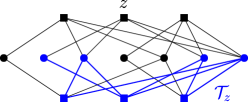
Definition 3.4 (Tanner cone-complex).
Let , be the Tanner graph of the code , with and . The Tanner cone-complex is the 2D simplicial complex888Here, by simplicial complex, we mean the geometrical realization of the associated abstract simplicial complex. This is because we will consider its fundamental group and do geometrical operations. In the abstract definition, a simplicial complex is a set of sets of objects called ”vertices”, which is closed under taking subsets. Every abstract simplicial complex defines a geometrical one, in which sets of 2 and 3 ”vertices” are respectively edges and triangular faces. The converse is also true. with 1-skeleton the graph , where
and with the set of triangular faces . In other words, there is at most a single edge between any pair of vertices corresponding to when their support has non-empty intersection. When it is clear from context that a Tanner cone-complex is associated to a code , we write it instead of .
Let represent the -matrix with rows indexed by the -checks and columns by the -checks, such that whenever the -th -check and the -th -check have a common support. Then the 1-skeleton of admits for adjacency matrix
Note that according to this definition, the Tanner cone-complex of any classical code satisfies .
While the construction of the Tanner cone-complex given in 3.4 is symmetric in and , we can also obtain it using the following method, which serves as an alternative definition. While Definition 3.4 is very simple, Proposition 3.6 highlights a property which will be central to show that the lift of a CSS code represents a valid code.
Definition 3.5.
Let and be spaces, being a subspace of , and denote the unit interval. The mapping cone of the inclusion map is the space obtained by attaching the cone on ,
to according to the equivalence , . It is noted .
Proposition 3.6.
Let . For any , let denote the subgraph induced by in . Then, for all we can consider the mapping cones of the inclusion maps , where denotes the cone on .
-
1.
The Tanner cone-complex is obtained by the attachment of all the cones on for , to at once,
-
2.
Exchanging the role of and checks, we also have
where is the subgraph induced by in .
Proof.
-
1.
We can label the vertex at the tip of by . Then, since every vertex in gives rise to an edge in when , we obtain all the edges connecting with qubits on which it has support and vertices of which have overlapping supports. Moreover, each edge gives rise to a face which has for boundary the path of edges .
-
2.
This is direct from Definition 3.4 of the Tanner cone-complex, which is symmetric in the sets of vertices and .∎
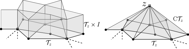
In Figure 2, we illustrate the construction of the Tanner cone-complex of Proposition 3.6. Note that for any vertex representing a or -check, is a contractible complex. This is a basic property of the cone, Definition 3.5 on a subcomplex.
Remark 3.7.
The Tanner cone-complex has the following noticeable features.
-
•
For any vertex representing a or stabilizer, its link999For any vertex of a regular cell complex , the link of in is defined as , where by we mean the cell defined by appending to the set of vertices defining . is .
-
•
For any vertex representing a qubit, is the complete bipartite graph composed of all the and vertices having support on (and all the edges between them).
Remark 3.8.
The Tanner cone-complex is the clique complex101010The clique complex of a graph is a simplicial complex in which every -vertex clique (every subset of vertices in which each pair of vertices are adjacent in ) of defines a dimensional cell in of its 1-skeleton. This is because any cycle of length 3 in its -skeleton is specified by a triple with , which also defines a face in the Tanner cone-complex.
This definition of Tanner cone-complex can be generalized to chain complex over -coefficients of any length. This is not needed in this work, but we state the definition for completeness.
Definition 3.9.
Consider the -chain complex , and denote the -th dual map . The Tanner graph is the graph with set of nodes , where elements of are identified with basis vectors of , and sets of edges , where there is an edge between and , iff .
The Tanner cone-complex is the 2D simplicial complex with set of edges , where , and sets of faces , where
It is then possible to give an alternative construction using the cone on induced subgraphs, similarly to Proposition 3.6.
3.3 Lift of a CSS code: definition
In this section, we define the lift of a CSS code. Intuitively, given a CSS code, one can consider covering maps of its Tanner cone-complex. It will first be shown that the associated covering space is the Tanner cone-complex of another CSS code. This new code will be defined as a lifted code. Then, the theory of covering maps can be used to classify all possible lifts.
The next proposition shows that a covering of any Tanner cone-complex can be used to define new quantum codes. This is not true in general if we try to do a covering of a Tanner graph directly, or of the 1-skeleton of the Tanner cone-complex. This is because for an arbitrary cover, the new induced subgraphs, see Definition 3.2, could be of odd degrees at certain check vertices. To understand this statement, consider two copies, noted and , of the Tanner graph of a CSS code . Select in the first graph an arbitrary vertex , a qubit vertex adjacent to that check, and the copy of these vertices , , in the second graph. Then, consider the graph obtained from the disjoint copies, by adding two edges and removing two others, . This is a 2-fold covering of the Tanner graph of , obtained by a permutation voltage. However, for any vertex such that in , the new subgraph induced by in is of odd degree at , so that does not satisfy Proposition 3.3. We can repeat the same kind of argument, if we consider covering of the 1-skeleton of . Therefore, to obtain a valid covering of a Tanner graph, another method is needed.
Theorem 3.10.
Let be a CSS code with Tanner graph and Tanner cone-complex . Any finite covering map of the Tanner cone-complex restricts to a covering map , for which the covering space represents the Tanner graph of a quantum CSS code , , with sets of checks , and qubits .
Proof.
We consider an arbitrary connected covering of the Tanner cone complex. Since we have the embedding of the Tanner graph as a subcomplex, and by Lemma 2.4, this covering map restricts to a covering map . We will show that satisfies the property of Proposition 3.3.
Let . The subcomplex is simply connected, since by construction the cone on a subcomplex can be retracted onto a point. The restriction of a covering map to a subcomplex of is also a covering of this subcomplex by Lemma 2.4. Hence, all the lifts of in must be disjoint copies of , that we denote as , where is an arbitrary indexing of the elements in the fiber above . Therefore, each of these subcomplex , for , corresponds to a new -generator , and it has as which is a subgraph of the 1-skeleton of . Therefore, , and in particular, it has even degree at the vertices of corresponding to preimage by of -vertices. We can repeat the same reasoning for all and subcomplexes . As mentioned in Proposition3.3, this is the only requirement for the 1-skeleton of to describe a valid Tanner graph, once we remove edges between check vertices to give for some code . ∎
In the rest of this article, we only consider CSS codes with connected Tanner graphs, since a code with a disconnected Tanner graph is a disjoint union of several codes, each of which can be studied independently. This is also a requirement for the fundamental group to be uniquely defined, up to isomorphism111111Given a basepoint on a topological space , recall that the fundamental group is the group of homotopy classes of loops based at , which has for group operation the concatenation of loops. For a space , and , ..
Definition 3.11 (lift of a CSS code).
Let be a CSS code, with Tanner graph , and Tanner cone-complex . Let be a finite cover of and its restriction to the Tanner graph. The lift of associated to corresponds to the CSS code such that (or equivalently with Tanner graph ), sets of checks , and qubits . A connected lift of is a lift defined by a connected cover of . A trivial lift of corresponds to disjoint copies of this code.
When a lift of a code is disconnected, one only obtains a disjoint union of codes, each of which is obtained by a connected lift of . For that reason, we restrict our attention to connected lifts.
Remark 3.12.
Notice that the fundamental group depends on the choice of basis of and -checks. For example, for the Toric code this is , but if we replace a basis check by , with such that , then this becomes the free product because, as seen in Proposition 3.6, we take the cone on a disconnected subgraph.
The condition for the existence of a non-trivial lift is the non triviality of . When this condition is satisfied, the lift of a CSS code possesses the following properties.
Proposition 3.13.
The lift of a quantum CSS code, associated to a degree covering of its Tanner cone-complex, enjoys the following properties.
-
1.
For an input CSS code of length , it is a CSS code of length given by .
-
2.
The maximum weight of rows and columns of the lifted check matrices is unchanged compared to that of the input code.
-
3.
The dimension of the new code is lower bounded by .
-
4.
If built from a finite regular cover, it has a free (linear) right action of the group of deck transformations and its dual complex has a similar left action.
-
5.
Applied to a classical code, it coincides with the geometrical lift of linear codes.
- 6.
Proof.
Items 1., 2. and follow from directly the theory of covering spaces. Item 3 comes from the cardinality of the fiber in a covering map and from a simple counting argument on the number of qubits and checks in the lifted code. Item 5. comes from the fact that the Tanner cone-complex of a linear code is simply its Tanner graph. Item 6. will be the subject of Section 4. ∎
Remark 3.14.
We are not aware of any method to compute the dimension and distance of a lifted code in full generality, given the parameters of an input code. This is at least as difficult as determining the 1st homology and the systole of a surface, since the Tanner cone-complex of a surface code is a simplicial refinement of a cellulation. For that reason, the strategy adopted later is a case by case study.
For example, several codes, such as Shor’s [36] and Steane’s [39] code, Quantum Reed-Muller codes121212Quantum Reed-Muller codes are non LDPC, and one check has support on every qubit. As a general rule, taking cones over large subgraphs of a graph is likely to trivialize the fundamental group of the whole graph., and quantum CSS codes from finite geometry [2] cannot be lifted in a non-trivial way because their Tanner cone-complexes have a trivial fundamental group. Some examples can be lifted in the usual sense: linear codes and codes coming from regular cellulations of surfaces.
Because the topological space is a connected cell complex, there is a way to classify all possible lifts of CSS codes. This is a direct consequence of the Galois correspondence, Theorem 2.7. More precisely, for every subgroup of there exists a path-connected covering space such that the . The new complex is the Tanner cone-complex of a lifted code , by Proposition 3.10. This statement of existence is essential, but we will not be interested in every subgroup of the fundamental group to create codes. Only subgroups of finite index in will give codes with a finite number of qubits.
Using this correspondence, it can be appropriate to denote the -lift of a CSS code . This is in contrast with the notation of Definition 2.11, where the -lift of a linear code is written , for an arbitrary choice of finite group , playing the role of the fiber of the covering. For a lifted CSS code, whenever we wish to put emphasis on the subgroup , we write in subscript. This notation is suitable when, for instance, the subgroup isn’t normal. However, when and we wish to put emphasis on the fiber of the covering , we write the lifted CSS code . This is useful when only a complicated presentation of is available, while the quotient group is well known.
3.4 Lift of a CSS code: explicit construction
In this section, we describe the procedure to construct the lift of a quantum CSS code explicitly. To this end, we first show how to produce a covering of the 1-skeleton of the Tanner cone-complex, which can be completed into a covering of the full complex. Since all the information about the lifted quantum code is contained in the 1-skeleton, we can derive the parity-check matrices of the lifted code from this graph covering. We keep the notations of graphs established in Section 2.5. Most of the material on covering maps and fundamental group is adapted from [26, 19], therefore the construction is detailed but proofs usually omitted.
We consider the CSS code and denote the dual maps for . Let , and . Recall that , the 1-skeleton of , is not isomorphic to since has edges between the and vertices.
The topological space is a finite connected simplicial complex. From the Galois correspondence, Theorem 2.7, connected coverings of the base space , are in one-to-one correspondence with subgroups of its fundamental group , where is an arbitrary choice of basepoint in that we now omit. In particular, let be a subgroup of . There exists a unique covering map,
| (12) |
associated to . It has degree . The lifted code is the one which satisfies , with the assignment of checks and qubits to vertices prescribed in Definition 3.11.
We will first construct the covering of Equation (12), by starting with a covering of the 1-skeleton of . To do so, we have to consider the following subgroups and homomorphisms,
where is the natural homomorphism, taking the quotient of by the normal closure131313Let be a presentation of a group . The normal closure of in , the free group generated by , is the smallest normal subgroup of containing , . Then, we have . of the subgroup generated by relations coming from loops which bound a face in . Moreover, is the preimage of in by this homomorphism. We now use the shorthand notations, and . Whenever is normal, there is an isomorphism . Otherwise, this is a bijection between the cosets, after specifying whether the cosets are taken from the left or right. Here, all cosets are taken on the right.
To construct the covering map , we must begin with a construction of the covering map
| (13) |
which exists and is also unique by Theorem 2.7. It can be obtained as the lift of a graph as exposed in Definition 2.9, but with a choice of voltage assignment specifically designed to produce connected coverings. We explain the steps to create and , the latter being a graph with sets of vertices that we now describe how to connect by edges. Since is a connected graph, it admits a maximal spanning tree with basepoint , and by definition a unique path from vertex to vertex. We define a specific type of voltage assignment on the set of oriented edges,
| (14) |
mapping an edge to an element of in the following manner. Let a path from vertex to be denoted as a sequence of oriented edges, for example . Moreover, let denote the path from to in the tree . Then the equivalence class of loops obtained by adding to is , where is the standard notation for the homotopy class of a loop based at . When we have an edge , we note , to make the notation less cluttered. We define a new construction of derived graphs associated to this voltage assignment.
Definition 3.15 (Connected lift of a graph).
Let be a connected graph, a spanning tree of , a voltage assignment on oriented edges as described above, a subgroup of and let . The right-derived graph is a graph with set of vertices and set of edges , so that a vertex or edge is written with and . An oriented edge in the graph , with and , connects and , where the multiplication by is always on the right.
In general, a graph admits more than one spanning tree. Following this procedure with another choice of spanning tree will modify the parametrization of the vertices and edges, but the graphs will be isomorphic, by the Galois correspondence.
When , this definition of lifts coincides with the one given in Definition 2.9 for the specific choice of voltage assignment given here. But while Definition 2.11 can generate all (connected and disconnected) regular covers, Definition 3.15 can generate all connected regular and non-regular covers.
With Definition 3.15 of right derived graph, we claim that . For that, we define as the map which projects any cell of , vertex or edge, to its first coordinate. This is a valid covering map, equivalent to what we have done in Section 2.5. It is also possible to prove that induces an isomorphism , for any choice of basepoint in the preimage of , by studying the image of loops in the cover (see [26], Chapter III. 3). Therefore, the graph and the map define the covering of Equation (13).
We could describe how to complete the covering of Equation (13) into the one of Equation (12) by geometrical means. But this step is not required to derive the boundary maps of the lifted code. Their expression is summarized in the next proposition.
Proposition 3.16.
Let be a CSS code, and denote the dual maps for . Let , a spanning tree of its 1-skeleton, a voltage assignment on oriented edges, and the natural homomorphism. For a given choice of subgroup with finite index, let be the associated lifted CSS code of . We write the set of -coset in . Then, this code can be written as
The boundary maps of the lifted code and its dual (in the sense of chain complex) are defined on basis elements of by
| (15) | ||||
where is any group element. Similarly, we have
| (16) | ||||
Their action is extended by linearity over chains.
Proof.
The dimension of each vector space of the lifted code is multiplied by the degree of the cover by Proposition 3.13; they are for the -checks, for the -checks and the qubits.
To express the boundary maps, we recall that the graph , with , carries all the data needed to construct the -lifted code of , since the new Tanner graph is just a subgraph of the 1-skeleton. We can determine new incidence matrices, , simply from the adjacency of vertices in . For instance, for they are written as follows on basis vectors, and , where . However, since we start from a choice of group , it is more adequate to use another parametrization of the fiber which depends on . For this, we make use of the natural homomorphism .
Proposition 3.10 ensures that the lifted boundary maps represent valid parity-check matrices for , and that . ∎
Finally, the total space of can be reconstructed from the definition of the Tanner cone-complex, with . The map then sends a face of , to . This ends the definition of the covering map.
3.5 Relation to the fiber bundle code
We have detailed a method to lift a CSS code via a connected covering of its Tanner cone-complex. We now explain how this is related to the fiber bundle code construction of [20].
The fiber bundle formulation of a lifted code is closely related to what we have done so far, but we need to restrict to normal covering maps and translate our formula to highlight the similarities. A normal covering map is also a principal -bundle , over a base space , with total space , fiber , a discrete group, on which a group acts freely and transitively. The group , called the structure group, is the group of automorphisms of the fiber. In our case, we consider covering maps over the base space . The fiber is the finite group , which is also the structure group.
Taking inspiration of principal -bundles, we can form an algebraic analogue, where the base space and fiber are replaced by two different chain complexes. The chain complex of the base space is the complex of the code . The fiber is the group ring , which may be extended into the trivial linear code . The action of on the fiber induces a linear action on the vector spaces of , since we have trivially , for any chain , and any .
The Tanner cone-complex , and hence the code , inherits the original free transitive linear left action of the group of deck transformations of the covering 141414we recall that the group of deck transformations is the group of homeomorphism with elements such that and is hence a free -module. Its dual complex enjoys a similar right action of . Taking advantage of that, it is possible to define a fiber bundle code [20], identified with the chain complex , for which the chain spaces are written
| (17) |
This is not the cellular chain complex151515The cellular chain complex of a cell complex is the chain complex indexed by dimension of cells, and whose -chains are formal combination of -dimensional cells, and boundary maps defined on a cell by formal sums of its boundary cells. of , which would have cells indexed by order of dimension. Equation (17) is a simple rewriting of a basis element into . To express the new boundary map we have to specify a chosen connection of the bundle, which is an assignment of a fiber automorphism element . Then, it is possible to make the parallel with the code of [20] more precise.
Proposition 3.17.
Suppose is a normal subgroup of . Then, the -lift of is identified with the fiber bundle code [20] , where . A connection is given on a pair by . On basis elements, the boundary maps read
| (18) | ||||
3.6 Relation to balanced product codes
In this section, we show how the lift is related to a certain balanced product operation, drawing a parallel with the construction in [3]. This is inspired by the algebraic approach to local systems of coefficients [12, 19], which already found applications in linear coding [29]. Usually, one defines a local coefficient system over the cellular chain complex of a space , with the help of a covering map. Here, we slightly revisit the procedure to define an analogue over an input code . Contrary to Section 3.5, this formulation is not restricted to the case of normal covering maps. In this section, we denote .
The Tanner cone-complex is a path connected space and has a universal cover, which coincides with the quotient map , where acts on the left by deck transformation. This complex is related to a specific code.
Definition 3.18.
Consider the CSS code , with having universal cover . We call the universal lift of , the chain complex , such that , , and .
Notice that we are careful not to call a code, unless each of its spaces has finite dimension. For the Toric code, the universal lift is the cellular chain complex of a cellulation of by finite-size squares.
Proposition 3.19.
For a CSS code , its universal lift is a chain complex of left -modules.
Proof.
From the theory of covering map, the free transitive left action of on induces a similar action of on the -cellular chain complex of (seen as a 2D simplicial complex), , endowing it with the structure of a module over the group algebra . The boundary maps of , noted , and its coboundary maps , become -module homomorphisms. This action of on , in turn, induces an action of on each vector space , defined by restricting the action of to the vertices of , interpreted as abstract cells of . This makes each space into a -module. The boundary maps are moreover -module homomorphisms. Indeed, they can be constructed from the boundary maps of in the following way. For and , we can interpret the cell both as a cell of or one of . Then the map satisfies where is the restriction map to the vertices representing cells (qubits) of , which is also a -module homomorphism. Therefore , making it a module homomorphism. The boundary map defined on basis vector by has the same property. The coboundary maps of can be obtained similarly.∎
Let be a discrete Abelian group over which the group acts on the left via a homomorphism . This endows with the structure of a left -module. Applying the tensor product with , seen as a -module, yield a -module, noted . For a cell complex , a local coefficient system on is defined as a complex of modules and morphisms . The tensor product of a left and a right -module has the effect of operating a change of ring. We now replace with , and consider a similar construction for the lifts of giving them a balanced product formulation.
Proposition 3.20.
Let be a CSS code with Tanner cone-complex , be a subgroup of and , the left cosets. Then we have an isomorphism of chain complexes,
| (19) |
Proof.
We keep the notation as in the proof of Proposition 3.19.
In the description of local systems, we take . This is an Abelian group, although is not necessarily a normal subgroup (in that case it corresponds to formal sums of coset elements). The ring can be endowed with the structure of a left -module, with the natural action of the fundamental group on the coset space. From the Galois correspondence is associated to a covering space and . For the present choice of , it can be shown that (see [19], Chapter 3.H).
Moreover, the left modules can be seen as right modules with the action on abstract chains . Therefore, the space is well-defined and can be both seen as a -module and a -module.
Each module of , and in particular the has a direct sum decomposition in terms of fibers of the covering map. As shown in the proof of Proposition 3.19, is constructed from by interpreting the cells of as abstract cells of , i.e. each fiber , where is given a unique type (, or ), depending on the type of . Therefore, we can also reconstruct each space by the span of the cells in , for interpreted as cells of , making it a subspace of stable under the action of . Then we form the chain complex by defining the boundary maps as in the proof of Proposition 3.19, i.e. and , which are also -module homomorphism. Therefore, tensoring it with the identity map on yields a unique -module homomorphism.∎
The cochain groups and maps can be defined by considering the dual spaces , the set of module homomorphisms from to .
Remark 3.21.
Because the cellular chain complex is a right -module, there is also a trivial balanced product relation, , corresponding to the space of coinvariants under the action of , see [3] Section IV.C.
4 Application to product codes
In this section, we analyze our construction for specific instances of input quantum CSS codes: hypergraph product codes. Then we present how the lift can be used as a first step to generate balanced product of quantum CSS codes.
4.1 Classification of lifts of HPC
Let be an HPC constructed from two classical codes and . These codes can be represented by their Tanner graphs and , which have free groups for fundamental group. Our first objective is to classify and analyze the codes that can obtained by lifts of HPC. The two main results of this section are Proposition 4.1 and 4.6. Proofs which do not appear in the present section are gathered in Appendix B. Here, the lower indices in do not point to the degree in the chain complex, but to a linear code labeled by .
Given a Cartesian product of two groups , Goursat quintuples are sets of the form , where for , and is an isomorphism. They serve to classify subgroups of , as described later.
Proposition 4.1.
Let be an HPC with and linear codes represented by their Tanner graphs and . Lifts of can be classified by the set of Goursat quintuples corresponding to finite index subgroups of , where , , and is an isomorphism.
The consequence of this proposition is the following. Given an HPC as above, with , and a covering map , associated to a subgroup , suppose cannot be decomposed as a Cartesian product of subgroups of the factors and . Then it is clear that cannot either be decomposed as a Cartesian product of two spaces, since is a free group. We can associate a certain lifted code to each of these non-product subgroups. Although this result was essentially obtained in [31], we show how to do this lift in the language of covering maps. This section hence establishes that our general notion of lift, Definition 3.11, agrees with the lifted product construction. All statements of this section related to fundamental group, covering spaces and group of deck transformations can be found in [19].
We first clarify how the Tanner cone complex of is related to the product of the Tanner graphs and .
Lemma 4.2.
The Tanner cone-complex of has .
Proof.
The Tanner cone-complex of is obtained from the 2D complex by dividing every square faces into 2 triangular cells by an edge connecting the and vertices at the corner of the faces. ∎
Lemma 4.3 (Goursat).
Let and be groups. There is a one-to-one correspondence between subgroups of and quintuples , where each , and is an isomorphism. It is given by .
Moreover, is a normal subgroup iff , are normal in and , the center of .
Proof.
For the full proof of this correspondence, see [1] Theorem 4, or [7] Section 2. Here we only outline the main steps leading to the definition of the bijection.
Let be a subgroup of . Define
| (20) | ||||
| (21) |
and write and similarly; they satisfy . It can be proved that , defined by for , is an isomorphism. Therefore, we obtain a map sending to the quintuple . Conversely, given the quintuple , we can check that is a subgroup of and therefore of . The correspondence is established by noticing that the two constructions are inverse of each other. ∎
We are now ready for the proof of Proposition 4.1.
Proof of Theorem 4.1.
Let be the Tanner cone-complex of , and . Then we know by Lemma 4.2 that . By the Galois correspondence, connected covering of are classified by subgroups of the fundamental group, which by Goursat Lemma 4.3 are classified by Goursat quintuples. Therefore, Goursat quintuples on yield a complete classification. ∎
The difficulty is to find families of codes related to these non product subgroups. In the following, we attempt to characterize and construct these subgroups. In our case, Goursat Lemma is applied for and free groups and therefore infinite. The next lemma implies that we can restrict our attention to the set of finite index subgroups and normal subgroups of free groups.
Lemma 4.4.
Let be a subgroup of corresponding to the quintuple . Then .
This is a classical result for finite groups, but as far the author knows, there is no standard reference treating the case of infinite groups. We therefore provide a proof in Appendix B.
From now on, we do not need the graphs to be bipartite for results to hold, unless it is clear from context that they should be interpreted as Tanner graphs of some linear codes. We explain a method to produce Goursat quintuples corresponding to finite index subgroups of , with and arbitrary finite graphs , for . Let and be two connected covering maps obtained from right derived graphs, generated by permutation voltage or (finite) group voltage. Therefore, and do not need to be regular, but they are finite and covers. Let be a finite group of order and for , be two voltage assignments. We note the right -lift of . The relations between these objects are summarized in the following diagram,
| (22) |
The next proposition indicates that Goursat quintuples of finite index subgroups can be obtained from the constituents of Equation (22).
Lemma 4.5.
Let and , for , be degree connected cover constructed as in Equation (22).
-
1.
Then, the quintuple , with , , and a choice of isomorphism, is a Goursat quintuple associated to a finite index subgroup of of index .
-
2.
Moreover, every Goursat quintuple can be obtained in this way.
-
3.
If is normal, then and are normal covers and is an Abelian cover, for .
While this statement appears direct, we still detail a proof, later in this section, using induced maps on fundamental groups. The aim is to better understand the correspondence between the geometrical object, the Goursat quintuple and lifts of graphs, which are central to prove other statements.
Note that it is straightforward to obtain a non-trivial Goursat quintuple with this method, i.e. one which is not a product of subgroups. It suffices to take a non-trivial finite group, so that is a proper subgroup of .
We now make a parallel between our approach and the lifted product construction of Panteleev and Kalachev [31].
Proposition 4.6.
Consider the subgroup associated to the quintuple . Let and let and , for , be connected cover constructed as above.
-
1.
The -cover of the product complex is normal iff is Abelian.
-
2.
The lifted code , with for , is equal to the product code obtained by lifting the classical codes according to .
The first claim of Lemma 4.6 is in accordance with a Remark 6 in [31]. In order to prove the results, we need to characterize more precisely the covering associated to a given Goursat quintuple.
Lemma 4.7.
Let be the subgroup of associated to the quintuple constructed as in Lemma 4.5, where we identify directly . Let be the set defined as follows . Then is a multiplicative group and is a covering map with
In other terms, Proposition 4.7 asserts the existence of a free transitive -action on and that . The action of is equivalent to a diagonal action of on each factor , where the first coordinate represents the -lift of a cell and the second coordinate represents the -lift of a cell .
Furthermore, let us consider the following application, , which as kernel . Supposing is normal in , is an epimorphism161616Surjective homomorphism. and by the first isomorphism theorem,
This provides a practical way to assign coordinates for the construction of . Let be a cell in . Then a cell in can be given by , where .
Our last corollary is a simple application of Proposition 4.6.
Corollary 4.8.
There exists a code (an HPC), and an indexed family of LDPC codes with parameters generated by the lift operations (covering maps) on the Tanner cone-complex .
The proof simply consists in translating the constituent of a lifted code in [31] into the present language of covering maps over Tanner graphs.
The procedure to obtain the boundary maps in the approach of Section 3.4 requires fixing a spanning tree in the Tanner cone-complex of . For completeness, we end this section by showing how to find an explicit spanning tree of a Cartesian product of graph by using the product structure.
We can proceed as follows. Let be a spanning tree of , ( is a subset of edges in and contains all the vertices). We consider the 1-skeleton of the Cartesian product . Then the following graph is a spanning tree of the Cartesian product ,
with an arbitrary choice of vertex in .
4.2 Balanced product of quantum CSS codes
The algebraic complex defined by the balanced product of chain complexes was identified in [3] to be of major importance in the theory of quantum codes. The lifted product of [32, 31] is in fact a particular case of balanced product complex. One difficulty addressed in this work, was the development of a systematic way of generating abstract 3-term chain complexes with a left or a right group action, which is a necessary ingredient to apply the balanced product to quantum codes.
Let and be two quantum CSS codes with Tanner cone-complex and . Let and be normal covering maps such that . The associated codes, which satisfy and , inherit the left action of the group of deck transformations, which is isomorphic for the two codes, . The action of is properly discontinuous, and the covering are respectively equivalent to . We can also define a right group action of the group of deck transformations by multiplying on the left by the inverse of a group element, or equivalently by the action of the opposite group .
The new codes are the chain complexes over , and . We can construct several new complexes out of these two chain complexes by considering them respectively as right and left -modules, following Section 3.5.
Definition 4.9.
The balanced product of quantum CSS codes is defined as the total complex of the tensor product double complex,
| (23) |
That is, it is the complex , with spaces indexed as
We can extract the 3-term complex , for which the constituent vector spaces are
| (24) | ||||
| (25) | ||||
| (26) |
The boundary maps are defined on an element by and extended by linearity over chains of .
Example 4.10.
The easiest variant of this construction involves , . More precisely we consider the product of a right -lift of and its dual , which inherits a right linear action of the group of deck transformations, .
Remark 4.11.
The balanced product of quantum CSS codes can be obtained from the left-right complex
for which we must give an interpretation to the sets of vertices as -checks, qubits and -checks.
5 New constructions and lifts
5.1 General method
In this section and the next, we introduce non-topological and non-product CSS code constructions which can be lifted into codes with improved parameters. We first explain the general procedure to produce them and, subsequently, we detail explicit examples and compute numerically parameters of some moderate-length lifted codes.
For any group , there exists at least one space which has for fundamental group [19]. When given a presentation , a possible construction of such space, called the presentation complex171717This complex is also related to the Cayley complex of . Let be the complex associated to a presentation . Then , where is the Cayley complex for this presentation. Moreover, is a covering map, and is the universal cover of . See [19], Section 1.3. associated to this presentation, goes as follows.
Lemma 5.1 ([19], Corollary 1.28. ).
For every group given with a presentation , there exists a 2-dimensional cell complex , the presentation complex, having 1 vertex, edges and 2-cells, with .
Proof.
Choose a presentation of , with and . This is the quotient of a free group on the generators of by the normal closure of the group generated by . The relations of are the generators of the kernel of the map . Now construct from a wedge of circles , by attaching one 2-cell, labeled , along the loops specified by the word . ∎
According to the construction given in the proof, if we suppose finitely presented, i.e. admits a presentation with and finite sets, then the associated presentation complex is a finite CW complex. Conversely, if the presentation isn’t finite, then the associated complex will have an infinite number of cells. Therefore, we focus on groups which are finitely presented.
Homotopy equivalent complexes can also be obtained easily. For example, by taking any other graph with fundamental group , one can add iteratively 2-cells in such a way that relations are added to the fundamental group until it is equal to . Alternatively, it is possible to refine the cellulation of the initial presentation complex of , in order to make it a regular CW complex. In each case, we can regard the obtained cellular chain complex as a quantum CSS code, in which the qubits are represented by the edges.
As we will see, a particularly interesting cellulation is one with 2-cells for which the boundary is a cycle of 4 edges. We call such a cellulation of a square cellulation , and we denote its 1-skeleton . When an instance is given, it is sometimes possible to make it finer and define a new abstract quantum code over that complex. By abstract, we mean a quantum code in which qubits and checks are not indexed by the dimension of cells181818There is always the FH-construction [13] which gives as 11-dimensional realization of a code into a manifold cellulation.. In this work, the codes are said to be of or -type, depending on whether qubits are placed on the edges or the vertices. An -type code simply refers to a topological code, i.e. a code equivalent to the -cellular chain complex of a regular 2-dimensional CW complex . But our intention is to present explicit and non-trivial -type codes, which are not equivalent to any topological code over a D complex.
Lemma 5.2.
There exists an infinite set of group presentations , with admitting a presentation complex which can be refined into a square cellulation and an assignment of checks and qubits to the vertices of , such that the associated -type code is not equal to any -type code over a cellulation of . Moreover, the Tanner cone-complex of this code is homeomorphic to .
More precisely, the Tanner cone-complex of this code is simply obtained from be subdividing each square 2-cell into 2 triangular cells in the right way, rendering the new complex simplicial.
The difficulty to construct such code lies in the fact that the -type code should not be equal to any -type code over . It is indeed always possible to find a square cellulation of a presentation complex and an assignment of checks and qubits to subsets of vertices, producing a valid CSS code. However, in most cases, the constructed quantum code is equal to an -type code. The proof of Lemma 5.2 consists of presenting specific groups for which the conditions are satisfied. For each of our case study, we first present these groups, labeled , and , from which we describe the presentation complex. We then define the codes , , and , , , and some specific instances of lift, obtained by covering of their Tanner cone-complex.
To compute subgroups and quotient groups, we use the GAP package LINS [15]. To compute an upper bound on the distances and , we use the GAP package [34], which operates with a probabilistic method based on information sets.
The criteria that we select to compare the performance of our codes is the quantity . For an HPC, it behaves asymptotically as when and , while for a good code, it increases as . For the rotated planar code [5], which is among the most considered codes for practical implementation, it is constant, with and .
5.2 Example 1: one-relator group
5.2.1 E-type code

In this section, we consider a one-relator group given with presentation
for . The associated presentation complex, labeled , is displayed in Figure 3 for and . To be precise, instead of starting from the presentation complex (built from a bouquet of 2 circles) we use a complex where 2 circles are linked by an edge. This modification being minor, we still refer to it as the presentation complex.
This construction is discussed in Examples 1.24 and 1.35 of [19]. Among its properties, we only mention that, when , are coprime, is a deformation retract of the complement of the -torus knot in , and when , are not coprime, cannot be embedded in .
We specify a regular cellulation of this topological space for each choice of and consider the code defined by its cellular chain complex.
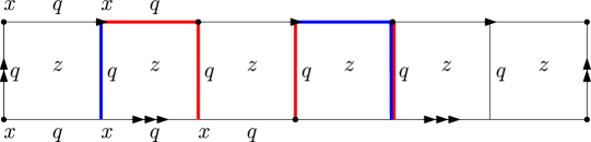
Definition 5.3.
Let be integers, , and be an integer. We define the code to be the cellular chain complex of the minimal cellulation with rows of square faces if , and faces if (see Figure 4 for ). The corresponding chain complex is , such that, if :
-
•
,
-
•
,
-
•
.
If :
-
•
,
-
•
,
-
•
.
In both cases:
-
•
,
-
•
,
-
•
,
-
•
.
In this work, as we only consider the case , we simply omit this parameter and note the code . Its presence in Definition 5.3 is merely intended to understand how cells are counted.
Lemma 5.4.
The dimension of is when is even, and otherwise.
Proof.
The highest nontrivial homology group is , with . This comes from the Hurewicz theorem, Theorem 2.5. Indeed, a presentation of the abelianization of is , which can be shown, in a few steps, to be equivalent to , by specifying and .
The dimension corresponds to the rank of . We compute this homology, starting from . The universal coefficient theorem states the existence of the short exact sequence
The Torsion term is defined as , where is a free (left) resolution of , the number of connected components of . This 0-th homology group being free, the resolution can be taken to be , with and is an isomorphism, implying that . This chain complex has only trivial maps and therefore no homology, rendering the torsion term trivial, which implies . Tensor product being distributive over direct sum of modules, and given that for any two integer , , we have if odd, and if even. ∎
Let be a finite index subgroup of . We define the code as the -lift of . Its dimension can be determined by applying Theorem 2.5, namely we start from , with the -cover of . Then, as in the proof of Lemma 5.4, the universal coefficient theorem yields .
There isn’t, to our knowledge, a specific mean of calculating the distance of a lifted code using geometric properties of the presentation complex. For that reason, we adopt a numerical approach and generate all lifts of degree 1 to 59 for . Table 1 gathers a selection of the lifts with the highest values of , although not exceeding 1.8. For , the set of lifts that we report has constant dimension but distance increasing with the length of the code. Most of the other lifts that we haven’t mentioned here had highly unbalanced and distances, leading to a poor .
| 3 | 3 | 5 | 1 | 0.4 | ||
| 12 | 1.8 | |||||
| 21 | 1.5 | |||||
| 24 | 1.5 | |||||
| 3 | 4 | 6 | 1 | 0.5 | ||
| 36 | 1.6 | |||||
| 48 | 1.5 | |||||
| 6 | 6 | 8 | 1 | 0.5 | ||
| 8 | 1 | |||||
| 12 | 1 | |||||
| 32 | 1 | |||||
| 40 | 1 |
5.2.2 V-type code
In this section, we modify the topological construction into a new abstract CSS code, i.e. one for which checks and qubits are no longer indexed by the dimension of topological cells.
Definition 5.5.
Let be integers, and be an integer. Consider a square cellulation with rows of 2-cells, and number of vertices if , and if . We define the code by assigning both qubits and checks to the vertices of in an alternating way, as shown in Figure 5, together with the identification . The corresponding chain complex is , such that, if :
-
•
,
-
•
,
-
•
.
If :
-
•
,
-
•
,
-
•
.
In both cases :
-
•
,
-
•
,
-
•
,
-
•
.

For , respectively , the code is topological and -checks, respectively -checks, can be viewed as faces. Apart from these choices, there are, a priori, no 2D cellular chain complex isomorphic to this code, since the (co)-boundary of a qubit has a weight greater than 2.
We emphasize the existence of a code having the following duality property.
Lemma 5.6.
For , there is an isomorphism .
Proof.
The code has the same number of qubits, and -checks. The isomorphism can be obtained by starting from , by translating all the vertex labels ( and ) horizontally by one position on the grid, and reflecting them with respect to the central horizontal line (which splits the sets of qubits into two sets of equal size). The obtained code is permutation-equivalent to the dual complex. ∎
In this work, as we only consider the case , we simply omit this parameter and note the code . It is specifically design to verify the following lemma.
Lemma 5.7.
There is an isomorphism .
Proof.
This is direct: the Tanner cone-complex corresponds to a triangulation of . ∎
Because this code is not a cellular chain complex, the lift presented in Section 3 is a particularly effective method to build codes of increasing size from a single input code.
As before, for a (finite index) subgroup of , we define the code as the -lift of . We generate numerically the lifts of degree 1 to 59 for and report parameters of input codes and lifted codes in Table 2. Notice that the dimension of the input codes behaves differently from the one of the -codes, which always have as shown in Lemma 5.4. Moreover, although the dimension of the input codes can vanish, this can change in the lifted codes191919Recall that our convention is to set when .. Overall, the parameters of the lifts here are greater than the ones of the -codes, which had not exceeding 1.8, and for several input codes we observe a noteworthy increase of this quantity.
| 3 | 3 | 5 | 1 | 0 | ||
| 9 | 1 | |||||
| 27 | 3 | |||||
| 3 | 4 | 6 | 1 | 0.3 | ||
| 48 | 2.3 | |||||
| 48 | 2.3 | |||||
| 4 | 4 | 6 | 1 | 0.4 | ||
| 32 | 2.4 | |||||
| 32 | 2.4 | |||||
| 4 | 5 | 7 | 1 | 0.5 | ||
| 20 | 2.9 | |||||
| 40 | 5.7 | |||||
| 4 | 6 | 8 | 1 | 0.3 | ||
| 48 | 2.3 | |||||
| 6 | 6 | 8 | 1 | 0.3 | ||
| 24 | 1.7 | |||||
| 6 | 7 | 9 | 1 | 0.5 | ||
| 42 | 6.8 |
5.3 Example 2: group presentation with more relations
5.3.1 E-type code
In this section, we consider a generalization of the previous codes. This is associated to the group given with presentation
for integers and . For , we have . The presentation complex , for the code , is depicted in Figure 6.
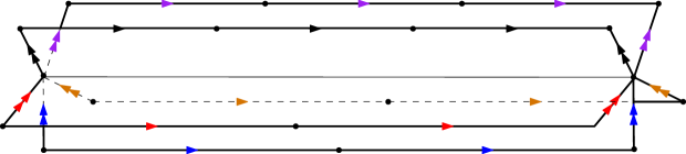
Using a square cellulation for this complex, we define the following topological code.
Definition 5.8.
Let , be integers, . Consider the square cellulation , for which each 2-cell of is subdivided into a row of square faces if , and square faces if . We define the code to be the cellular chain complex of . The corresponding chain complex is , such that, if :
-
•
,
-
•
,
-
•
.
If :
-
•
,
-
•
,
-
•
.
In both cases:
-
•
,
-
•
,
-
•
,
-
•
.
Note that here, in contrast to , we only consider the case (number of rows of 2-cells). This is because otherwise the number of qubits would increase linearly in both and .
Remark 5.9.
We could consider even more general groups, for which each generator has its own independent exponent, . Both for simplicity and economy of qubits, we reduce the possible choices by setting and . Indeed, otherwise the number of qubits would scale as .
5.3.2 V-type code: symmetric version
There are two ways to define an abstract code from the presentation complex of . In this section, we consider a version that we refer to as symmetric, because under specific choices of integers , the chain complex of the code can be made isomorphic to its dual.
Definition 5.10.
Let , be integers and . Consider the square cellulation , constructed by starting with the one of Definition 5.8, to which we add a row of square 2-cells in between the faces coming from relations and the one coming from relations . We define the code by assigning both qubits and checks to the vertices of in an alternating way as shown in Figure 7, together with the identification . The corresponding chain complex is , such that, if :
-
•
,
-
•
,
-
•
.
If :
-
•
,
-
•
,
-
•
.
In both cases:
-
•
,
-
•
,
-
•
,
-
•
.
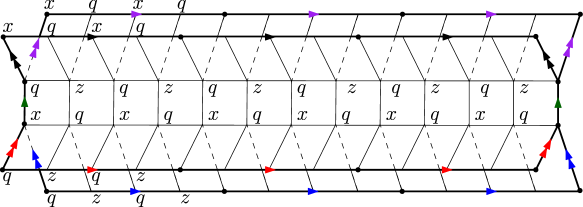
Among these constructions, we emphasize the existence of the codes when , such as , which have the same number of and -checks. Another code of interest has the following duality property.
Lemma 5.11.
For and , we have .
Proof.
The code has the same number of and -checks. The isomorphism can be obtained by starting from , translating all the vertex labels horizontally by one position, and reflecting them with respect to the central horizontal line which splits the sets of qubits into two sets of equal size. This is permutation-equivalent to the dual complex. ∎
By construction, the Tanner cone-complex of these code satisfies the following lemma.
Lemma 5.12.
There is an isomorphism .
Proof.
This is direct: the Tanner cone-complex corresponds to a triangulation of . ∎
For or , this code cannot be associated to any cellular chain complex of a D complex because of the value taken by and . Therefore, the lift of Definition 3.11 is a pertinent method to generate new codes. For a (finite index) subgroup of , we define the code as the -lift of . We report parameters of 2 selected lifted codes in Table 3, due to the enormous amount of subgroups of , that we could not to investigate in its entirety. Observe that, while the relative distance of the -lift is lower than the one we had for the -lift of the -code, the quantity is increased by a factor of 2 due to the change of . This suggests that, by adding few qubits in the input code, as controlled by the value of , the quantity of logical qubits stored in a lifted code can increase drastically.
| 3 | 3 | 2 | 2 | 5 | 1 | 0.4 | ||
| 9 | 2 | |||||||
| 4 | 4 | 2 | 2 | 6 | 1 | 0.7 | ||
| 12 | 2.1 |
5.3.3 V-type code: asymmetric version
In this section, we consider a restriction of the group and a variation of the previous code. For clarity, we define a new group given with the presentation
In particular, we have . Therefore, the presentation complex for this code is constructed similarly to the previous one. Using a square cellulation for this complex, we define a new -type code.
Definition 5.13.
Let be integers. Consider the cellulation , constructed by subdividing each 2-cell of into square faces. We define the code by assigning both qubits and checks to the vertices of , such that -checks are assigned to vertices of the central circle, alternating with qubits as shown in Figure 8, other qubits and -checks being assigned accordingly, together with the identification . The corresponding chain complex is , with number of qubits and checks:
-
•
,
-
•
,
-
•
.
The weights of parity-check matrices are:
-
•
,
-
•
,
-
•
,
-
•
.
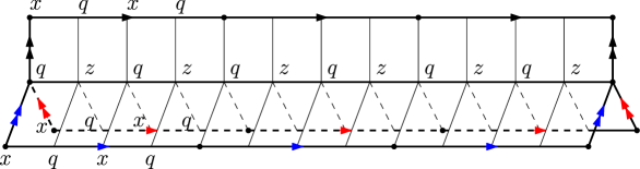
For , respectively , this code is topological and -checks, respectively -checks, can be viewed as faces. More precisely, for , this code is . Aside from these choices, there are no 2D cellular chain complex isomorphic to this code. Nevertheless, its Tanner cone-complex still satisfies the following lemma.
Lemma 5.14.
There is an isomorphism .
Proof.
The Tanner cone-complex is the triangulation obtain from by subdividing each face by a diagonal edge. ∎
Let be a (finite index) subgroup of . We define the code as the -lift of and report parameters of a selection of lifted codes in Table 4. We only mention a few due to the enormous set of subgroups of , that we were not able to investigate in its entirety. Notice that the values of (and ) for the and -lifts of are slightly increased compared with the corresponding lifts of .
| 3 | 3 | 5 | 1 | 0.7 | ||
| 9 | 2.7 | |||||
| 27 | 4 | |||||
| 4 | 3 | 6 | 1 | 0.9 | ||
| 42 | 2.7 |
6 Discussion and perspectives
This work started the investigation of lifted codes beyond LPCs. In Section 3, we have given a definition of the lift based on the idea of covering of the Tanner cone-complex and in Section 5, we introduced a method to construct liftable CSS codes based on the presentation complex of certain groups. Let us now give a few comments and new directions.
Firstly, there might exist alternative approaches to lift a CSS code, possibly generalizing Definition 3.11. There are, undoubtedly, coverings of the Tanner graph of a given CSS code, which represent valid codes and cannot be obtained as the lifts of the Tanner cone-complex. We believe that such notions might rely more on the use of an algebraic structure rather than geometrical ones.
Secondly, we have only introduced examples of non-topological codes associated to a specific instances of the group presentation of Section 5.3. At the time of the writing, we are aware of other group presentations yielding non-topological liftable codes, but these codes, being of much greater length, are challenging to investigate numerically. It is therefore necessary to understand the behavior of the dimension and distance of a given lifted code analytically. Nevertheless, a less ambitious goal is to devise new examples of moderate length codes, based on certain group presentations, in order to improve on the codes presented here. The parameters exposed in Tables 2, 3 and 4 are indeed very far from the ones of the recently introduced group algebra codes [24], or even Abelian lifted product codes [30]. Notice, however, that we have only dealt with regular coverings of the Tanner cone-complex, while, as shown in Section 4, the asymptotically good codes are obtained as non-regular coverings of HPCs.
Finally, while it seems that the V-type codes and are likely to reach interesting parameters at moderate length, we haven’t been able to analyze all the lifts, due to the very large amount of them. There is therefore a potential need to generate them by other means. For example, a simple method to produce a subset of them is as follows: given copies of , we can create a lift of by gluing them along the inverse image (by the covering map) of the central circle in . We can do a similar construction of certain lifts of , starting with copies of . We leave a more rigorous description and analysis of these codes for future work.
Acknowledgement
The author would like to thank Benjamin Audoux and Anthony Leverrier for valuable discussions throughout this work, as well as for carefully reading and commenting the manuscript. The author would also like to thank Allen Hatcher for answering a question on a forum. We acknowledge the Plan France 2030 through the project NISQ2LSQ ANR-22-PETQ-0006.
References
- AC [09] D. D. Anderson and V. Camillo. Subgroups of direct products of groups, ideals and subrings of direct products of rings, and Goursat’s lemma, 2009.
- AC [19] Benjamin Audoux and Alain Couvreur. On tensor products of CSS codes. Annales de l’Institut Henri Poincaré D, Combinatorics, Physics and their Interactions, 6(2):239–287, March 2019.
- [3] Nikolas P. Breuckmann and Jens N. Eberhardt. Balanced Product Quantum Codes. IEEE Transactions on Information Theory, 67(10):6653–6674, October 2021.
- [4] Nikolas P. Breuckmann and Jens Niklas Eberhardt. Quantum Low-Density Parity-Check Codes. PRX Quantum, 2(4), October 2021.
- BMD [07] H. Bombin and M. A. Martin-Delgado. Optimal resources for topological two-dimensional stabilizer codes: Comparative study. Physical Review A, 76(1), July 2007.
- Bro [82] Kenneth S. Brown. Some Homological Algebra, pages 4–32. Springer New York, New York, NY, 1982.
- BSZ [11] Kristine Bauer, Debasis Sen, and Peter Zvengrowski. A Generalized Goursat Lemma, 2011.
- CS [96] A. R. Calderbank and Peter W. Shor. Good quantum error-correcting codes exist. Physical Review A, 54(2):1098–1105, August 1996.
- CW [75] R. R. Crawford and K. D. Wallace. On the Number of Subgroups of Index Two-An Application of Goursat's Theorem for Groups. Mathematics Magazine, 48(3):172, May 1975.
- DEL+ [21] Irit Dinur, Shai Evra, Ron Livne, Alexander Lubotzky, and Shahar Mozes. Locally Testable Codes with constant rate, distance, and locality, 2021.
- DHLV [23] Irit Dinur, Min-Hsiu Hsieh, Ting-Chun Lin, and Thomas Vidick. Good Quantum LDPC Codes with Linear Time Decoders. In Proceedings of the 55th Annual ACM Symposium on Theory of Computing, STOC 2023, page 905–918, New York, NY, USA, 2023. Association for Computing Machinery.
- DK [01] James F. Davis and Paul A. Kirk. Lecture notes in algebraic topology. 2001.
- FH [21] Michael Freedman and Matthew Hastings. Building manifolds from quantum codes. Geometric and Functional Analysis, 31(4):855–894, June 2021.
- FM [01] Michael H. Freedman and David A. Meyer. Projective Plane and Planar Quantum Codes. Foundations of Computational Mathematics, 1(3):325–332, July 2001.
- GAP [24] The GAP Group. GAP – Groups, Algorithms, and Programming, Version 4.13.0, 2024.
- Gou [89] Edouard Goursat. Sur les substitutions orthogonales et les divisions régulières de l’espace. Annales scientifiques de l’École Normale Supérieure, 3e série, 6:9–102, 1889.
- GT [77] Jonathan L. Gross and Thomas W. Tucker. Generating all graph coverings by permutation voltage assignments. Discrete Mathematics, 18(3):273–283, 1977.
- Gue [24] Virgile Guemard. Geometric approach to lift from the Freedman-Hastings construction. 2024.
- Hat [02] Allen Hatcher. Algebraic topology. Cambridge University Press, Cambridge, 2002.
- HHO [21] Matthew B. Hastings, Jeongwan Haah, and Ryan O’Donnell. Fiber bundle codes: breaking the n1/2 polylog(n) barrier for Quantum LDPC codes. In Proceedings of the 53rd Annual ACM SIGACT Symposium on Theory of Computing, STOC 2021, page 1276–1288, New York, NY, USA, 2021. Association for Computing Machinery.
- Joh [90] F. E. A. Johnson. On normal subgroups of direct products. Proceedings of the Edinburgh Mathematical Society, 33(2):309–319, June 1990.
- Kit [03] A.Yu. Kitaev. Fault-tolerant quantum computation by anyons. Annals of Physics, 303(1):2–30, January 2003.
- LH [22] Ting-Chun Lin and Min-Hsiu Hsieh. Good quantum LDPC codes with linear time decoder from lossless expanders, 2022.
- LP [24] Hsiang-Ku Lin and Leonid P. Pryadko. Quantum two-block group algebra codes. Physical Review A, 109:022407, Feb 2024.
- LPS [88] A. Lubotzky, R. Phillips, and P. Sarnak. Ramanujan graphs. Combinatorica, 8(3):261–277, September 1988.
- LS [01] Roger C. Lyndon and Paul E. Schupp. Combinatorial Group Theory. Springer Berlin Heidelberg, 2001.
- LZ [22] Anthony Leverrier and Gilles Zémor. Quantum Tanner codes. In FOCS 2022 - IEEE 63rd Annual Symposium on Foundations of Computer Science, pages 872–883, Denver, United States, October 2022. IEEE.
- LZ [23] Anthony Leverrier and Gilles Zémor. Decoding quantum tanner codes. IEEE Transactions on Information Theory, 69(8):5100–5115, 2023.
- Mes [18] Roy Meshulam. Graph codes and local systems, 2018.
- PK [21] Pavel Panteleev and Gleb Kalachev. Degenerate Quantum LDPC Codes With Good Finite Length Performance. Quantum, 5:585, November 2021.
- [31] Pavel Panteleev and Gleb Kalachev. Asymptotically good Quantum and locally testable classical LDPC codes. In Proceedings of the 54th Annual ACM SIGACT Symposium on Theory of Computing, STOC ’22. ACM, June 2022.
- [32] Pavel Panteleev and Gleb Kalachev. Quantum ldpc codes with almost linear minimum distance. IEEE Transactions on Information Theory, 68(1):213–229, 2022.
- PK [24] Pavel Panteleev and Gleb Kalachev. Maximally extendable sheaf codes, 2024.
- PSK [22] Leonid P. Pryadko, Vadim A. Shabashov, and Valerii K. Kozin. QDistRnd: A GAP package for computing the distance of quantum error-correcting codes. Journal of Open Source Software, 7(71):4120, 2022.
- PSVC [11] Ali E. Pusane, Roxana Smarandache, Pascal O. Vontobel, and Daniel J. Costello. Deriving Good LDPC Convolutional Codes from LDPC Block Codes. IEEE Transactions on Information Theory, 57(2):835–857, 2011.
- Sho [95] Peter W. Shor. Scheme for reducing decoherence in quantum computer memory. Physical Review A, 52(4):R2493–R2496, October 1995.
- SS [96] M. Sipser and D.A. Spielman. Expander codes. IEEE Transactions on Information Theory, 42(6):1710–1722, 1996.
- [38] A. M. Steane. Error Correcting Codes in Quantum Theory. Physical Review Letters, 77(5):793–797, July 1996.
- [39] A. M. Steane. Multiple-particle interference and quantum error correction. Proceedings of the Royal Society of London. Series A: Mathematical, Physical and Engineering Sciences, 452(1954):2551–2577, November 1996.
- Tan [81] Robert Michael Tanner. A recursive approach to low complexity codes. IEEE Trans. Inf. Theory, 27:533–547, 1981.
- Tho [03] J. Thorpe. Low-Density Parity-Check (LDPC) Codes Constructed from Protographs. Interplanetary Network Progress Report, 42-154:1–7, August 2003.
- TZ [09] Jean-Pierre Tillich and Gilles Zemor. Quantum LDPC codes with positive rate and minimum distance proportional to , 2009.
- ZP [19] Weilei Zeng and Leonid P. Pryadko. Higher-Dimensional Quantum Hypergraph-Product Codes with Finite Rates. Phys. Rev. Lett., 122:230501, Jun 2019.
Appendix A Further restrictions on covering maps
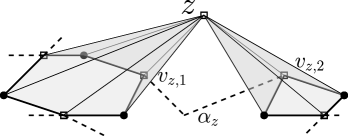
In general, for a code with and , some of the induced subgraphs for , or for , and even the Tanner graphs , can be disconnected. This happens, for instance, in Shor’s -qubit code [36]. In this case, when we create the Tanner cone-complex following Proposition 3.6, taking the cone on a disconnected subgraph produces new generators in the fundamental group of the complex.
Lemma A.1.
Suppose has disjoint components, and . There exists a subgroup , such that
This has no impact on the definition of the lift given in Definition 3.11, but when doing numerical studies, it can be desirable to produce coverings of according to subgroups of not involving these generators. To this end, we can trivialize the corresponding generators of the fundamental group by adding new faces in . In the following procedure, these faces have usually more than 3 edges in their boundaries. Let be such that is disconnected, as illustrated in Figure 9, then
-
1.
Choose a basepoint for each connected component of .
-
2.
For each connected component of , fix an embedded simply-connected path in , going from subgraphs to subgraphs, through each basepoint. For a specific component of containing connected components of , label the basepoints according to this path , by specifying the starting and end points.
-
3.
For each reduced subpath of between and , add a (non-triangular) face along the loop formed by , the subpath from to and .
-
4.
Repeat steps 1. to 3. for all connected component of and and for all with disconnected induced subgraphs.
We call the result . According to Lemma 2.4, any covering of defines one for , but not the other way around. Then, everything in Section 3.4 remains true if we replace with .
Appendix B Proofs for Section 4.1
We now proceed with the proof of each statement of Section 4.1.
Proof (of Lemma 4.4):.
See [9] Corollary 4, when the groups are finite. From Lemma 4.3, has its elements from the set . The index is the number of -cosets in .
Let be an element in a -coset. We change coset if we multiply by an element not in . According to the definition, fixing , we change -coset every time we change -coset, and there are of them for each -coset. Therefore, there are -cosets. The second equality is obtained by considering the symmetric definition of the set of , since is an isomorphism.∎
Proof (of Lemma 4.5).
-
1.
The covering space being a right -lift of , it has a discontinuous and free left -action. Therefore, is the finite regular cover with . Moreover, this cover is associated to the subgroup of and . We hence have a first isomorphism .
From the theory of covering maps, the cover being finite connected, it is associated to a finite index subgroup of and there is an isomorphism from onto this subgroup, identified with . Choosing the normal subgroup of , this induces another isomorphism . Composing this isomorphism with , we have an isomorphism
defined as .
The covering map being also finite connected, the composition is a well-defined degree covering map and induces a homomorphism . This chain of isomorphisms defines triples, , as in the proposition. All these subgroups being associated to finite covers, they have finite index in and are free groups of finite rank given by
Therefore is a valid isomorphism which defines a Goursat quintuple as claimed.
It is straightforward to determine the index of the subgroup associated to this quintuple. Indeed and . From, Lemma 4.4, the associated subgroup is of index .
-
2.
Let be any Goursat quintuples of the product of free groups, and let be a graph with . We know from [17] that every subgroup of can be obtained as an element for some permutation voltage of such that the associated cover is connected. Moreover, we have access to all normal subgroups of by creating normal connected covers with group voltage of . Therefore, we can obtain all subgroups of in the form of , for some . It only remains to fix an isomorphism equal to .
-
3.
To obtain a normal subgroup , it is also necessary for and to be connected regular covers. This is direct from the correspondence established in the proof of the 1st claim and Lemma 4.3. Therefore, can also be obtained from a finite connected -lift of for some group . Moreover, since we must have , then needs to be Abelian. Notice however that it is not a sufficient condition.∎
Proof (of Proposition 4.7).
First, it is easily verified that but in general is not a normal subgroup of unless is a normal subgroup. According to Lemma 2.8, is a normal cover with group of deck transformations and therefore .
It is straightforward to see, from the definition of , that but we give several steps for completeness. Indeed, let , then is not a homomorphism, but its restriction to is a surjective one. can be decomposed as with , which are also not homeomorphism. For an element , , we show that any element in the preimage is in . Indeed, let and then . Moreover and , hence and . Moreover, let , Then, and let us call . Since is an isomorphism, we have the unique identification . Hence, each element is mapped surjectively by onto an element , and we showed that . Therefore .
We proceed to show that . Indeed, the main covering gives the isomorphism and a chain of covering yields the isomorphism , and . We look at the homomorphism where is the restriction of to . The map is an injective homomorphism, but its restriction to its image is an isomorphism onto , and is surjective. Therefore, is an epimorphism and it is direct to compute its kernel. Indeed, yields . Therefore, by the first isomorphism theorem,
This finishes the proof by reminding that the l.h.s is isomorphic to and the r.h.s is . ∎
It is now possible to prove the equivalence between the lifted product code and the lift of a quantum code stated in Proposition 4.6
Proof (of Proposition 4.6).
-
1.
In this setting the subgroups satisfy , hence the covering maps are trivial and in particular normal. For the cover of to be normal, we require , which in this case is reduced to , and therefore .
-
2.
There is an obvious similarity between the geometrical complexes which represent the code and . The Tanner graph of is the 1-skeleton of the complex while the Tanner graph of is the 1-skeleton of the complex . These graphs are the same because , with the relation
and the equivalence on the r.h.s is the one defining . The CSS codes represented by these Tanner graphs are equal if the interpretation that we make of subsets of vertices as qubits, -checks and -checks are the same. Let and denote the sets of respectively check nodes and bit nodes in . The condition is satisfied as for both graphs, the set of qubits is identified with the set , and the set of checks is identified with the set . ∎
Proof (of Corollary 4.8).
Let , , be the bipartite graph with 2 vertices, noted and , and edges connecting them. This is the graph considered in [31], in which bit variables are assigned to the edges, and parity-checks to the vertices. Let denote the Tanner graphs of these codes , where each edge in has been split in two by a bit vertex . For each bit vertex we call left and right the edges with endpoint respectively the vertex and . The code corresponds to .
Let , be two parity-check matrices verifying the condition in the proof of Proposition 1 of [31] and be the Tanner graph of the Tanner code [37] defined by the graph and the local codes , . We can infer a covering of from one of , reproducing the Tanner code over the Cayley graph with Ramanujan properties [25] used in [31]. For this, we create a covering of from a specific voltage assignment.
Notice that in the Tanner code construction, each edge or in is replaced by a group of left or right edges or . Let denotes the voltage assignment on giving rise to the derived graph and , the one in . If assigns element to running from to , then assigns the same element to all edges of running from to and the identity element to edges of . With this choice of , the derived graph of the cover is equal to the Tanner graph of .
We can then use the covering as described in Proposition 4.6 to create the code .∎