History Repeats Itself: A Baseline for Temporal Knowledge Graph Forecasting

Abstract

Temporal Knowledge Graph (TKG) Forecasting aims at predicting links in Knowledge Graphs for future timesteps based on a history of Knowledge Graphs. To this day, standardized evaluation protocols and rigorous comparison across TKG models are available, but the importance of simple baselines is often neglected in the evaluation, which prevents researchers from discerning actual and fictitious progress. We propose to close this gap by designing an intuitive baseline for TKG Forecasting based on predicting recurring facts. Compared to most TKG models, it requires little hyperparameter tuning and no iterative training. Further, it can help to identify failure modes in existing approaches. The empirical findings are quite unexpected: compared to 11 methods on five datasets, our baseline ranks first or third in three of them, painting a radically different picture of the predictive quality of the state of the art.

1 Introduction

The lack of experimental rigor is one of the most problematic issues in fast-growing research communities, producing empirical results that are inconsistent or in disagreement with each other. Such ambiguities are often hard to resolve in a short time frame, and they eventually slow down scientific progress. This issue is especially evident in the machine learning field, where missing experimental details, the absence of standardized evaluation protocols, and unfair comparisons make it challenging to discern true advancements from fictitious ones Lipton and Steinhardt (2019).

As a result, researchers have spent considerable effort in re-evaluating the performances of various models on different benchmarks, to establish proper comparisons and robustly gauge the benefit of an approach over others. In recent years, this was the case of node and graph classification benchmarks Shchur et al. (2018); Errica et al. (2020), link prediction on Knowledge Graphs Sun et al. (2020); Rossi et al. (2021), neural recommender systems Dacrema et al. (2019), and temporal graph learning Huang et al. (2023).

Not only does such fast growing literature impact reproducibility and replicability, but it is also characterized by a certain forgetfulness that simple baselines set a threshold above which approaches are actually useful. Oftentimes, these baselines are missing from the empirical evaluations, but when introduced they provide a completely new picture of the state of the art. Examples can be found in the field of Knowledge Graph completion, where simple rule-based systems can outperform embedding-based ones Meilicke et al. (2018), or in graph-related tasks where structure-agnostic baselines can compete with deep graph networks Errica et al. (2020); Poursafaei et al. (2022); Errica (2023).

In the last few years, the field of Temporal Knowledge Graph (TKG) Forecasting has also experienced a fast-paced research activity culminating in a large stream of works and a variety of empirical settings Liu et al. (2022); Sun et al. (2021); Zhang et al. (2023). Researchers have already provided a thorough re-assessment of some TKG Forecasting methods to address growing concerns about their reproducibility, laying down a solid foundation for future comparisons Gastinger et al. (2023). What is still missing, however, is a comparison with simple baselines to gauge if we are really making progress and to identify pain points of current representation learning approaches for TKGs.

Our contribution aims at filling this gap with a novel baseline, which places a strong inductive bias on the re-occurrence of facts over time. Not only does our baseline require tuning of just two hyperparameters, but also no training phase is needed since it is parameter-free. We introduce three variants of the baseline, divided into strict recurrency, relaxed recurrency, and a combination of both. Our empirical results convey an unexpected message: the baseline ranks first and third on three out of five datasets considered, compared to 11 TKG methods. It is a perhaps unsurprising result, given the long history of aforementioned works that propose strong baselines in different communities, but it further highlights the compelling need for considering simple heuristics in the TKG forecasting domain. Finally, by carefully comparing the performance of these baselines with other methods, we provide a failure analysis that highlights where it might be necessary to improve existing models.

2 Related Work

In this section, we give a concise overview of the plethora of TKG forecasting methods that appeared in recent years.

Deep Graph Networks (DGNs)

Several models in this category leverage message-passing architectures Scarselli et al. (2009); Micheli (2009) along with sequential approaches to integrate structural and sequential information for TKG forecasting. RE-Net adopts an autoregressive architecture, learning temporal dependencies from a sequence of graphs Jin et al. (2020). RE-GCN combines a convolutional DGN with a sequential neural network and introduces a static graph constraint to consider additional information like entity types Li et al. (2021b). xERTE employs temporal relational attention mechanisms to extract query-relevant subgraphs Han et al. (2021a). TANGO utilizes neural ordinary differential equations and DGNs to model temporal sequences and capture structural information Han et al. (2021b). CEN integrates a convolutional neural network capable of handling evolutional patterns in an online setting, adapting to changes over time Li et al. (2022b). At last, RETIA generates twin hyperrelation subgraphs and aggregates adjacent entities and relations using a graph convolutional network Liu et al. (2023a).

Reinforcement Learning (RL)

Methods in this category combine reinforcement learning with temporal reasoning for TKG forecasting. CluSTeR employs a two-step process, utilizing a RL agent to induce clue paths and a DGN for temporal reasoning Li et al. (2021a). Also, TimeTraveler leverages RL based on temporal paths, using dynamic embeddings of the queries, the path history, and the candidate actions to sample actions, and a time-shaped reward Sun et al. (2021).

Rule-based

Rule-based approaches focus on learning temporal logic rules. TLogic learns these rules via temporal random walks Liu et al. (2022). TRKG extends TLogic by introducing new rule types, including acyclic rules and rules with relaxed time constraints Kiran et al. (2023). ALRE-IR combines embedding-based and logical rule-based methods, capturing deep causal logic by learning rule embeddings Mei et al. (2022). LogE-Net combines logical rules with RE-GCN, using them in a preprocessing step for assisting reasoning Liu et al. (2023b). At last, TECHS incorporates a temporal graph encoder and a logical decoder for differentiable rule learning and reasoning Lin et al. (2023).

Others

There are additional approaches with mixed contributions that cannot be immediately placed in the above categories. CyGNet predicts future facts based on historical appearances, employing a ”copy” and ”generation” mode Zhu et al. (2021). TiRGN employs a local encoder for evolutionary representations in adjacent timestamps and a global encoder to collect repeated facts Li et al. (2022a). CENET distinguishes historical and non-historical dependencies through contrastive learning and a mask-based inference process Xu et al. (2023). Finally, L2TKG utilizes a structural encoder and latent relation learning module to mine and exploit intra- and inter-time latent relations Zhang et al. (2023).

3 Approach

This section introduces several baselines: We start with the Strict Recurrency Baseline, before moving to its “relaxed” version, the Relaxed Recurrency Baseline, and, ultimately, a combination of the two, the so-called Combined Recurrency Baseline. Before we introduce these baselines, we give a formal definition of the notion of a Temporal Knowledge Graph and and provide a running example to illustrate our approach.

3.1 Preliminaries

A Temporal Knowledge Graph $G$ is a set of quadruples $(s,r,o,t)$ with $s,o\in E$, relation $r\in R$, and time stamp $t\in T$ with $T=\{1\ldots n\},n\in\mathbb{N}^{+}$. More precisely, $E$ is the set of entities, $R$ is the set of possible relations, and $T$ is the set of timesteps. A quadruple’s $(s,r,o,t)$ semantic meaning is that $s$ is in relation $r$ to $o$ at $t$. Alternatively, we may refer to this quadruple as a temporal triple that holds during the timestep $t$. This allows us to talk about the triple $(s,r,o)$ and its occurrence and recurrence at certain timesteps. In the following, we use a running example $G$, where $G$ is a TKG in the soccer domain shown in Figure 1. $G$ contains triples from the years 2001 to 2009, which we map to indices 1 to 9.

⬇

(marta, playsFor, vasco-da-gamah, 1)

(marta, playsFor, vasco-da-gamah , 2)

(marta, playsFor, santa-cruz, 3)

(marta, playsFor, santa-cruz, 4)

(marta, playsFor, umea-ik, 5)

(marta, playsFor, umea-ik, 6)

(marta, playsFor, umea-ik, 7)

(marta, playsFor, umea-ik, 8)

(marta, playsFor, los-angeles-sol, 9)

Figure 1: A (slightly simplified) listing of the clubs that Marta Vieira da Silva, known as Marta, played for from 2001 to 2009.

Temporal Knowledge Graph Forecasting is the task of predicting quadruples for future timesteps ${t^{+}}$ given a history of quadruples $G$, with ${t^{+}}>n$ and ${t^{+}}\in\mathbb{N}^{+}$. In this work we focus on entity forecasting, that is, predicting object or subject entities for queries $(s,r,?,{t^{+}})$ or $(?,r,o,{t^{+}})$. Akin to KG completion, TKG forecasting is approached as a ranking task Han (2022). For a given query, e.g. $(s,r,?,{t^{+}})$, methods rank all entities in $E$ using a scoring function, assigning plausibility scores to each quadruple.

In the following, we design several variants of a simple scoring function $f$ that assigns a score in $\mathbb{R^{+}}$ to a quadruple at a future timestep ${t^{+}}$ given a Temporal Knowledge Graph $G$, i.e., $f((s,r,o,{t^{+}}),G)\mapsto\mathbb{R^{+}}$. All variants of our scoring function are simple heuristics to solve the TKG forecasting task, based on the principle that something that happened in the past will happen again in the future.

3.2 Strict Recurrency Baseline

The first family of recurrency baselines checks if the triple that we want to predict at timestep ${t^{+}}$ has already been observed before. The simplest baseline of this family is the following scoring function $\phi_{1}$:

$$\phi_{1}((s,r,o,{t^{+}}),G)=\begin{cases}1,&\text{if}\ \exists k\ \text{with}\ (s,r,o,k)\in G\\ 0,&\text{otherwise.}\end{cases}$$ (1)

If we apply $\phi_{1}$ to the set of triples in Figure 1 to compute the scores for 2010, we get the following outcome (using pf to abbreviate playsFor).

$$\phi_{1}((\texttt{\footnotesize marta},\texttt{\footnotesize pf},\texttt{\footnotesize vasco-da-gamah},\texttt{\footnotesize 10}),G)=1$$

$$\phi_{1}((\texttt{\footnotesize marta},\texttt{\footnotesize pf},\texttt{\footnotesize santa-cruz},\texttt{\footnotesize 10}),G)=1$$

$$\phi_{1}((\texttt{\footnotesize marta},\texttt{\footnotesize pf},\texttt{\footnotesize umea-ik},\texttt{\footnotesize 10}),G)=1$$

$$\phi_{1}((\texttt{\footnotesize marta},\texttt{\footnotesize pf},\texttt{\footnotesize los-angeles-sol},\texttt{\footnotesize 10}),G)=1$$

This scoring function suffers from the problem that it does not take the temporal distance into account, which is highly relevant for the relation of playing for a club. It is far more likely that Marta will continue to play for Los Angeles Sol rather than sign a contract with a previous club.

To address this problem, we introduce a time weighting mechanism to assign higher scores to more recent triples. Defining a generic function $\Delta:\mathbb{N}^{+}\times\mathbb{N}^{+}\rightarrow\mathbb{R}$ that takes the query timestep ${t^{+}}$, a previous timestep $k$ in $G$, and returns the weight of the triple, we can define strict recurrency scoring functions as follows:

$$\phi_{\Delta}((s,r,o,{t^{+}}),G)=\begin{cases}\Delta({t^{+}},\max\{k|(s,r,o,k)\in G\})\\ 0,\ \ \ \text{if}\ \nexists k\ \text{with}\ (s,r,o,k)\in G.\end{cases}$$ (2)

For instance, using $\Delta^{0}({t^{+}},k)=k/{t^{+}},k<{t^{+}}$ produces:

$$\phi_{\Delta^{0}}((\texttt{\footnotesize marta},\texttt{\footnotesize pf},\texttt{\footnotesize vasco-da-gamah},\texttt{\footnotesize 10}),G)=0.2$$

$$\phi_{\Delta^{0}}((\texttt{\footnotesize marta},\texttt{\footnotesize pf},\texttt{\footnotesize santa-cruz},\texttt{\footnotesize 10}),G)=0.4$$

$$\phi_{\Delta^{0}}((\texttt{\footnotesize marta},\texttt{\footnotesize pf},\texttt{\footnotesize umea-ik},\texttt{\footnotesize 10}),G)=0.8$$

$$\phi_{\Delta^{0}}((\texttt{\footnotesize marta},\texttt{\footnotesize pf},\texttt{\footnotesize los-angeles-sol},\texttt{\footnotesize 10}),G)=0.9,$$

which already makes more sense: the latest club that a person played for will always receive the highest score.

Interestingly, we can establish an equivalence class among a subset of the functions $\phi_{\Delta}$, and we will use this fact in our experiments. As long as we solely focus on ranking results, two scoring functions are equivalent if they define the same partial order over all possible temporal predictions.

Definition 1.

Two scoring functions $\phi$ and $\phi^{\prime}$ are ranking-equivalent if for any pair of predictions $p=(s,r,o,{t^{+}})$ and $p^{\prime}=(s^{\prime},r^{\prime},o^{\prime},{t^{+}})$ we have that $\phi(p,G)>\phi(p^{\prime},G)\iff\phi^{\prime}(p,G)>\phi^{\prime}(p^{\prime},G)$.

The next result states that we do not need to search for an optimal time weighting function $\Delta({t^{+}},k)$ if we choose it to be strictly monotonically increasing with respect to $k$, as these functions belong to the same equivalence class.

Proposition 1.

Scoring functions $\phi_{\Delta}$ and $\phi_{\Delta^{\prime}}$ are ranking equivalent iff, $\forall\ k_{1},k_{2},{t^{+}}$ such that $k_{1}<k_{2}<{t^{+}}$ it holds $\Delta({t^{+}},k_{1})<\Delta({t^{+}},k_{2})$ and $\Delta^{\prime}({t^{+}},k_{1})<\Delta^{\prime}({t^{+}},k_{2})$.

Proposition 1 follows from the application of Definition 1. Therefore, the set of functions $\phi_{\Delta}$, characterized by a $\Delta$ that is strictly monotonically increasing in $k$, are ranking equivalent.

While $\phi_{\Delta}$ works well to predict the club that a person will play for, there are relations with different temporal characteristics. An example might be a relation that expresses that a soccer club wins a certain competition. In Figure 2, we extend our TKG with temporal triples using the relation wins.

⬇

(fc-bayern-munich, wins, bundesliga, 1)

(borussia-dortmund, wins, bundesliga, 2)

(fc-bayern-munich, wins, bundesliga, 3)

(werder-bremen, wins, bundesliga, 4)

(fc-bayern-munich, wins, bundesliga, 5)

(fc-bayern-munich, wins, bundesliga, 6)

(vfb-stuttgart, wins, bundesliga, 7)

(fc-bayern-munich, wins, bundesliga, 8)

(vfl-wolfsburg, wins, bundesliga, 9)

Figure 2: Clubs winning the Bundesliga from 2001 to 2009.

The relation wins seems to follow a different pattern compared to the previous example. Indeed, applying $\phi_{\Delta^{0}}$ to predict the 2010 winner of the Bundesliga would not reflect the fact that FC Bayern Munich is the club with the highest ratio of won championships, and year 9 might just have been a lucky one for VFL Wolfsburg. The frequency of wins could be considered a better indicator for a scoring function:

$$\psi_{1}((s,r,o,{t^{+}}),G)=|\{k\ |\ (s,r,o,k)\in G\}|/{t^{+}}$$ (3)

Based on this scoring function, the club that has won the most titles, Bayern Munich, receives the highest score of $0.6$, while all other clubs receive a score of $0.1$.

As done earlier, we now generalize the formulation of $\psi_{1}$ to $\psi_{\Delta}$ using a weighting function $\Delta({t^{+}},k)$ where triples that occurred more recently are weighted higher:

$$\psi_{\Delta}((s,r,o,{t^{+}}),G)=\frac{\sum_{i\in\{k\mid(s,r,o,k)\in G\}}\Delta({t^{+}},i)}{\sum_{i=1}^{n}\Delta({t^{+}},i)}.$$ (4)

Again, we apply the new scoring functions to our example. We shortened the names of the clubs and abbreviated bundesliga as bl:

$$\psi_{\Delta^{0}}((\texttt{\footnotesize dortmund},\texttt{\footnotesize wins},\texttt{\footnotesize bl},\texttt{\footnotesize 10}),G)=0.2/4.5\approx 0.04$$

$$\psi_{\Delta^{0}}((\texttt{\footnotesize bremen},\texttt{\footnotesize wins},\texttt{\footnotesize bl},\texttt{\footnotesize 10}),G)=0.4/4.5\approx 0.09$$

$$\psi_{\Delta^{0}}((\texttt{\footnotesize stuttgart},\texttt{\footnotesize wins},\texttt{\footnotesize bl},\texttt{\footnotesize 10}),G)=0.7/4.5\approx 0.15$$

$$\psi_{\Delta^{0}}((\texttt{\footnotesize munich},\texttt{\footnotesize wins},\texttt{\footnotesize bl},\texttt{\footnotesize 10}),G)=2.3/4.5\approx 0.51$$

$$\psi_{\Delta^{0}}((\texttt{\footnotesize wolfsburg},\texttt{\footnotesize wins},\texttt{\footnotesize bl},\texttt{\footnotesize 10}),G)=0.9/4.5\approx 0.2$$

It is worth noting that, for a restricted family of distributions $\Delta^{\prime}(t,k)$, we can achieve ranking equivalence between scoring functions $\psi_{\Delta^{\prime}}$ and $\phi_{\Delta}$ with a strictly increasing $\Delta(t,k)$. More specifically, if we make $\Delta^{\prime}(t,k)$ parametric, then $\psi_{\Delta^{\prime}}$ can generalize the family of scoring functions $\phi_{\Delta}$. Consider the parameterized function $\Delta_{\lambda}({t^{+}},k)=2^{\lambda(k-{t^{+}})}$ with $\lambda\in\mathbb{R}_{0}^{+}$, where $\lambda$ acts as a decay factor. The higher $\lambda$, the stronger the decay effect we achieve. In particular, if we set $\lambda=1$, we can enforce that a time point $k$ always receives a higher weight than the sum of all previous time points $1,\ldots,k-1$. This means $\psi_{\Delta_{1}}$ and $\phi_{\Delta}$ are ranking equivalent.

Proposition 2.

For $\lambda\geq 1$, $\Delta_{\lambda}=2^{\lambda(k-{t^{+}})}$, and any strictly increasing time weighting function $\Delta$, the scoring functions $\phi_{\Delta}$ and $\psi_{\Delta_{\lambda}}$ are ranking equivalent.

Proposition 2 follows directly from the fact that $\sum_{i=k+1}^{n}\frac{1}{2^{i}}<\frac{1}{2^{k}}$ for any $n>k\in\mathbb{N}^{+}$.

On the contrary, we get ranking equivalence between $\psi_{1}$ and $\psi_{\Delta_{\lambda}}$ if we set $\lambda=0$.

Proposition 3.

The scoring functions $\psi_{1}$ and $\psi_{\Delta_{\lambda}}$ are ranking equivalent if we set $\lambda=0$.

Proposition 3 follows directly from $2^{0}=1$ and the definition of $\psi_{1}$ in Equation 3. Propositions 2 and 3 help us to interpret our experimental results, as it indicates that different settings of $\lambda$ result in a scoring function that is situated between $\psi_{1}$ and $\phi_{\Delta_{\lambda}}$. We treat $\lambda$ as a relation-specific hyperparameter in our experiments, meaning we will select a different $\lambda_{r}$ for each relation $r$. Since relations are independent of each other, each $\lambda_{r}$ can be optimized independently.

3.3 Relaxed Recurrency Baseline

So far, our scoring functions were based on a strict application of the principle of recurrency. However, this approach fails to score a triple that has never been seen before, and we need to account for queries of this nature: imagine a young player appearing for the first time in a professional club.

Thus, we introduce a relaxed variant of the baseline. Instead of looking for exact matching of triples in previous timesteps, which would not work for unseen triples, we are interested in how often parts of the triple have been observed in the data. When asked to score the query $(s,r,?,{t^{+}})$, we compute the normalized frequency that the object $o$ has been in relationship $r$ with any subject $s^{\prime}$:

$$\overrightarrow{\xi}((s,r,o,{t^{+}}),G)=\frac{|\{(s^{\prime},k)\ |\ (s^{\prime},r,o,k)\in G\}|}{|\{(s^{\prime},o^{\prime},k)\ |\ (s^{\prime},r,o^{\prime},k)\in G\}|}$$ (5)

Analogously, we denote with $\overleftarrow{\xi}((s,r,o,{t^{+}}),G)$ the relaxed baseline used to score queries of the form $(?,r,o,{t^{+}})$. In the following, we omit the arrow above $\xi$ and use the directed version depending on the type of query without explicit reference to the direction.

Let us revisit the example of Figure 1 and apply $\xi$ to score a triple never seen before. We can now assign non-zero scores to the clubs that Aitana Bonmati, who never appeared in $G$, will likely play for in 2010:

$$\xi((\texttt{\footnotesize bonmati},\texttt{\footnotesize pf},\texttt{\footnotesize vasco-da-gamah},\texttt{\footnotesize 10}),G)=0.22$$

$$\xi((\texttt{\footnotesize bonmati},\texttt{\footnotesize pf},\texttt{\footnotesize santa-cruz},\texttt{\footnotesize 10}),G)=0.22$$

$$\xi((\texttt{\footnotesize bonmati},\texttt{\footnotesize pf},\texttt{\footnotesize umea-ik},\texttt{\footnotesize 10}),G)=0.44$$

$$\xi((\texttt{\footnotesize bonmati},\texttt{\footnotesize pf},\texttt{\footnotesize los-angeles-sol},\texttt{\footnotesize 10}),G)=0.11$$

While we also report results for $\xi$ on its own, we are mainly interested in its combination with the the Strict Recurrency Baseline, where we expect it to fill up gaps and resolve ties. For simplicity, we do not introduce a weighted version of this baseline to avoid the extra hyperparameter.

3.4 Combined Recurrency Baseline

We conclude the section with a linear combination of the Strict Recurrency Baseline $\psi_{\Delta_{\lambda}}$ and the Relaxed Recurrency Baseline $\xi$. In particular (omitting $\lambda$ to keep the notation uncluttered):

$$\begin{split}\psi_{\Delta}\xi((s,r,o,{t^{+}}),G)=\alpha*\psi_{\Delta}(s,r,o,{t^{+}}),G)+\\ (1-\alpha)*\xi(s,r,o,{t^{+}}),G),\end{split}$$ (6)

where $\alpha\in[0,1]$ is another hyperparameter. Similar to $\lambda$, we select a different $\alpha_{r}$ for each relation $r$. In the following, we refer to this baseline as the Combined Recurrency Baseline.

4 Experimental Setup

This section describes our experimental setup and provides information on how to reproduce our experiments. We rely on the unified evaluation protocol of Gastinger et al. (2023), reporting results about single-step predictions. We report results for the multi-step setting in the supplementary material.

4.1 Hyperparameters

We select the best hyperparameters by evaluating the performances on the validation set as follows: First, we select $\lambda_{r}\forall r\in R$ from in total 14 values, $\lambda_{r}\in L_{r}=\{0,...,1.0001\}$ for $\psi_{\lambda}$. Then, after fixing the best $\lambda_{r}\forall r\in R$, we select $\alpha_{r}\forall r\in R$ from 13 values, $\alpha_{r}\in A_{r}=\{0,...,1\}$, leading to a total of 27 combinations per relation.

4.2 Methods for Comparison

We compare our baselines to 11 among the 17 methods described in Section 2. Two of these 17 methods run only in multi-step setting, see comparisons to these in the supplementary material. Further, for four methods we find discrepancies in the evaluation protocol and thus exclude them from our comparisons. Unless otherwise stated, we report the results for these 11 methods based on the evaluation protocol by Gastinger et al. (2023). For TiRGN, we report the results of the original paper and do a sanity check of the released code. We do the same for L2TKG, LogE-Net, and TECHS, but we cannot do a sanity check as their code has not been released.

4.3 Dataset Information

We assess the performance of the recurrency baselines on five datasets Gastinger et al. (2023); Li et al. (2021b), namely WIKI, YAGO, ICEWS14, ICEWS18, and GDELT. Table 1 shows characteristics such as the number of entities and quadruples, and it reports the timestep-based data splitting (short: #Tr/Val/Te TS) all methods are evaluated against. In addition, we compute the fraction of test temporal triples $(s,r,o,{t^{+}})$ for which there exists a $k<{t^{+}}$ such that $(s,r,o,k)\in G$, and we refer to this measure as the recurrency degree (Rec). Similarly, we also compute the fraction of temporal triples $(s,r,o,{t^{+}})$ for which it holds that $(s,r,o,{t^{+}}-1)\in G$, which we call direct recurrency degree (DRec). Note that Rec defines an upper bound of Strict Recurrency Baseline’s performance; instead, DRec informs about the test triples that have, from our baselines’ perspective, a trivial solution. On YAGO and WIKI, both measures are higher than 85%, meaning that the application of the recurrency principle would likely work very well.

Dataset	$\#$Nodes	$\#$Rels	$\#$Train	$\#$Valid	$\#$Test	Time Int.	$\#$Tr/Val/Te TS	DRec [%]	Rec [%]
ICEWS14	$7128$	$230$	$74845$	$8514$	$7371$	24 hours	304/30/31	10.5	52.4
ICEWS18	$23033$	$256$	$373018$	$45995$	$49545$	24 hours	239/30/34	10.8	50.4
GDELT	$7691$	$240$	$1734399$	$238765$	$305241$	15 min.	2303/288/384	2.2	64.9
YAGO	$10623$	$10$	$161540$	$19523$	$20026$	1 year	177/5/6	92.7	92.7
WIKI	$12554$	$24$	$539286$	$67538$	$63110$	1 year	210/11/10	85.6	87.0

Table 1: We report some statistics of the datasets, the timestep interval, and the specifics of the data splitting. We also include the recurrency degree (Rec) and the direct recurrency degree (DRec). Please refer to the text for a more detailed description.

4.4 Evaluation Metrics

As is common in link prediction evaluations, we focus on two metrics: the Mean Reciprocal Rank (MRR), computing the average of the reciprocals of the ranks of the first relevant item in a list of results, as well as the Hits at 10 (H@10), the proportion of queries for which at least one relevant item is among the top 10 ranked results. Following Gastinger et al. (2023), we report the time-aware filtered MRR and H@10.

5 Experimental Results

This section reports our quantitative and qualitative results, illustrating our baselines help to gain a deeper understanding of the field. We list runtimes in the Supplementary Material.

5.1 Global Results

	GDELT		YAGO		WIKI		ICEWS14		ICEWS18
	MRR	H@10	MRR	H@10	MRR	H@10	MRR	H@10	MRR	H@10
L2TKG†	20.5	35.8	-	-	-	-	47.4	71.1	33.4	55.0
LogE-Net†	-	-	-	-	-	-	43.7	63.7	32.7	53.0
TECHS†	-	-	89.2	92.4	76.0	82.4	d.d.v	d.d.v.	30.9	49.8
TiRGN	21.7	37.6	88.0	92.9	81.7	87.1	44.0	63.8	33.7	54.2
TRKG	21.5	37.3	71.5	79.2	73.4	76.2	27.3	50.8	16.7	35.4
RE-GCN	19.8	33.9	82.2	88.5	78.7	84.7	42.1	62.7	32.6	52.6
xERTE	18.9	32.0	87.3	91.2	74.5	80.1	40.9	57.1	29.2	46.3
TLogic	19.8	35.6	76.5	79.2	82.3	87.0	42.5	60.3	29.6	48.1
TANGO	19.2	32.8	62.4	67.8	50.1	52.8	36.8	55.1	28.4	46.3
Timetraveler	20.2	31.2	87.7	91.2	78.7	83.1	40.8	57.6	29.1	43.9
CEN	20.4	35.0	82.7	89.4	79.3	84.9	41.8	60.9	31.5	50.7
Relaxed ($\xi$)	14.2	23.6	5.2	10.7	14.3	25.4	14.4	28.6	11.6	22.0
Strict ($\psi_{\Delta}$)	23.7	38.3	90.7	92.8	81.6	87.0	36.3	48.4	27.8	41.4
Combined ($\psi_{\Delta}\xi$)	24.5	39.8	90.9	93.0	81.5	87.1	37.2	51.8	28.7	43.7

Table 2: Experimental results. An entry ${\dagger}$ means authors have not released their code, and thus we could not reproduce their results, an entry - that the related work does not report results on this dataset, and an entry ”d.d.v”, that the it reports results on a different dataset version.

Table 2 (lower area) shows the MRR and H@10 results for the Strict ($\xi$), the Relaxed ($\psi_{\Delta}$), and the Combined Recurrency Baseline ($\psi_{\Delta}\xi$). For all datasets, with one minor discrepancy, the Combined Recurrency Baseline performs better than the strict and the relaxed variants. However, the Strict Recurrency Baseline is not much worse: The difference to the Combined Recurrency Baseline is for both metrics never more than one percentage point. We observe that, while $\xi$ scores a MRR between $5\%$ and $15\%$ on its own, when combined with $\psi_{\Delta}$ (thus obtaining $\psi_{\Delta}\xi$) it can grant up to $0.9\%$ of absolute improvement. As described in Section 3, its main role is to fill gaps and resolve ties. The results confirm our intuition. Interestingly, results for $\psi_{\Delta}\xi$ on all datasets reflect the reported values of the recurrency degree and direct recurrency degree (see Table 2): For both YAGO and WIKI (Rec and DRec $>85\%$), our baseline yields high MRRs ($>80\%$), while in other cases the values are below $40\%$.

When compared to results from related work (upper area of Table 2), the Combined Recurrency Baseline as well as the Strict Recurrency Baseline yield the highest test scores for two out of five datasets (GDELT and YAGO) and the third-highest test scores for the WIKI dataset. This is an indication that most related work models seem unable to learn and consistently apply a simple forecasting strategy that yields high gains. In particular, we highlight the significant difference between the Combined Recurrency Baseline and the runner-up methods for GDELT (with a relative change of $+12.9\%$).

Results for ICEWS14 and ICEWS18, instead, suggest that more complex dependencies need to be captured on these datasets. While two methods (TRKG and TANGO) perform worse than our baseline, the majority achieves better results.

In summary, none of the methods proposed so far can accomplish the results achieved by a combination of two very naïve baselines for two out of five datasets. This result is rather surprising, and it raises doubts about the predictive quality of current methods.

5.2 Per-Relation Analysis

We conduct a detailed per-relation analysis and focus on two datasets: ICEWS14, since our baseline performed worse there, and YAGO, for the opposite reason. We compare the Combined Recurrency Baseline to the four methods that performed best on the respective dataset, considering the seven methods evaluated under the evaluation protocol of Gastinger et al. (2023). For clarity, we adopt the following notation to denote a relation and its prediction direction: [relation] (head) signifies predictions in head direction, corresponding to queries of the form $(?,r,o,{t^{+}})$; [relation] (tail) denotes predictions in tail direction, i.e., $(s,r,?,{t^{+}})$.

ICEWS14

In Figure 3(a), we focus on the nine most frequent relations. For each relation, one or multiple methods reach MRRs higher than the Combined Recurrency Baseline, with an absolute offset in MRR of approximately $3\%$ to $7\%$ between the best-performing method and our baseline. This indicates that it might be necessary to capture patterns going beyond the simple recurrency principle. However, even for ICEWS14, we see three relations where some methods produce worse results than the Combined Recurrency Baseline. For two of these (Make_a_visit, Host_a_visit), RE-GCN and CEN attain the lowest MRR. In the third relation (Arrest_detain_or_charge_with_legal_action), TLogic and xERTE have the lowest MRR. This implies that, despite having better aggregated MRRs, the methods display distinct weaknesses and are not learning to model recurrency for all relations.

(a) ICEWS14

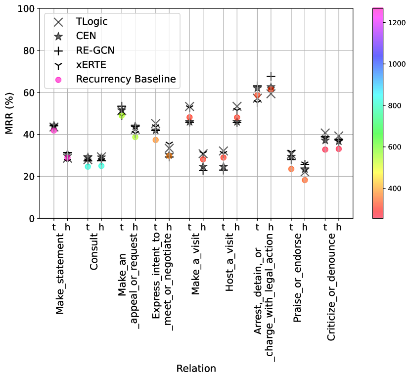
(b) YAGO

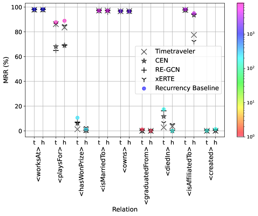
Figure 3: Test MRRs for each relation and direction (“t” means tail and “h” head, respectively) for (a) ICEWS14 (top) and (b) YAGO (bottom). Colors indicate the number of queries for relation and its direction in the test set.

YAGO

Figure 3(b), instead, shows two distinct categories of relations: the first category contains relations where most methods demonstrate competitive performance (MRR$\geq 85\%$). In all of them, the Combined Recurrency Baseline attains the highest scores. Thus, the capabilities of related work, like detecting patterns across different relations or multiple hops in the KG, do not seem to be beneficial for these relations, and a simpler inductive bias might be preferred. The second category contains relations where all methods perform poorly (MRR $\leq 20\%$). Due to the dataset’s limited information, reliably predicting prize winners or deaths is unfeasible. For these reasons, we expect no significant improvement in future work on YAGO beyond the results of our baseline.

However, YAGO still provides value to the research field: it can be used to inspect the methods’ capabilities to identify and predict simple recurring facts and, if this is not the case, to pinpoint their deficiencies. Thus, YAGO can be also seen as a dataset for sanity checks. All analysed methods from related work fail this sanity check: none of them can exploit the simple recurrency pattern for all relations. The main disparity in overall MRR between the Combined Recurrency Baseline and related work can be attributed to two specific relations: playsFor (head, tail), and isAffiliatedTo (head). Queries attributed to these relations make for almost $50\%$ of all test queries. More specifically, Timetraveler exhibits limitations with isAffiliatedTo (head) and playsFor (head); xERTE shows its greatest shortcomings for isAffiliatedTo (head); and RE-GCN and CEN exhibit limitations with the relation playsFor in both directions. These findings highlight the specific weaknesses of each method that are possible by comparisons with baselines, thus allowing for targeted improvements.

5.3 Failure Analysis

In the following, we analyse some example queries where the recurrency principle offers an unambiguous solution which, however, is not chosen by a specific method. Following Section 5.2, we focus on YAGO and the same four models. We base our analysis on the insights that YAGO has a very high direct recurrency degree, and that predicting facts based on strict recurrency with steep time decay leads to very high scores. The MRR of $\phi_{\Delta}$ is $90.7\%$. For each model, we count for how many queries the following conditions are fulfilled, given the test query $(s,r,?,t)$ with correct answer $o$: (i) $(s,r,o,t\!-\!1)\in G$, (ii) the model proposed $o^{\prime}\neq o$ as top candidate, (iii) there exists no $k$ with $(s,r,o^{\prime},k)\in G$. If these are fulfilled, there is strong evidence for $o$ due to recurrency, while $(s,r,o^{\prime})$ has never been observed in the past. We conduct the same analysis for head queries $(?,r,o,t)$. For each model, we randomly select some of these queries and describe the mistakes made.

Timetraveler

Surprisingly, Timetraveler sometimes suggests top candidates that are incompatible with respect to domain and range of the given relation, even when all above conditions are met. Here are two examples for the ”playsFor” (pf) relation, where the proposed candidates are marked with a question mark:

$$(\texttt{\footnotesize?=spain-national-u23},\texttt{\footnotesize pf},\texttt{\footnotesize lierse-sk},\texttt{\footnotesize 10})$$

$$(\texttt{\footnotesize?=baseball-ground},\texttt{\footnotesize pf},\texttt{\footnotesize derby-county-fc},\texttt{\footnotesize 10})$$

The reasons behind Timetraveler’s predictions, despite the availability of reasonable candidates according to the recurrency principle, fall outside the scope of this paper.

xERTE

For xERTE, we detect a very clear pattern that explains the mistakes. In 147 out of 149 cases, xERTE predicts a candidate as subject (object) $c$ when $c$ was given as object (subject). This happens in nearly all cases for the symmetric relation isMarriedTo resulting in the prediction of triples such as $(john,isMarriedTo,john)$. This error pattern bears a striking resemblance to issues observed in the context of non-temporal KG completion in Meilicke et al. (2018) where it has already been argued that some models perform surprisingly badly on symmetric relations.

CEN and RE-GCN

Both CEN and RE-GCN exhibit distinct behavior. Errors frequently occur with the ”playsFor” relation, particularly in tail prediction. In all analysed examples, the types (soccer players and soccer clubs) of the incorrectly predicted candidates were correct. Moreover, we cannot find any other systematic error pattern or explanation for the erroneous predictions. It seems that both models are not able to learn that the playsFor relation follows the simple regularity of strict recurrency, even though this regularity dominates the training set.

These examples highlight significant insights into the current weaknesses of each method. Future research can leverage these insights to enhance the affected models.

5.4 Parameter Study

In the following, we summarize our findings regarding the influence of hyperparameters on baseline predictions. Detailed results are provided in the Supplementary Material.

5.4.1 Influence of Hyperparameter Values

We analyze the impact of $\lambda$ and $\alpha$ on overall MRR. Notably, $\lambda$ significantly affects the MRR, e.g., with test results ranging from $12.1\%$ to $23.7\%$ for GDELT across different $\lambda$ values. The optimal $\lambda$ varies across datasets. This underlines the influence of time decay: Predicting repetitions of the most recent facts is most beneficial for YAGO and WIKI, while also considering the frequency of previous facts is better for the other datasets. This distinction is also mirrored in the direct recurrency degree, being notably high for YAGO and WIKI, and thus indicating the importance of the most recent facts. Additionally, setting $\alpha$ to a high value ($\alpha\geq 0.99$) yields the best aggregated test results across all datasets, indicating the benefits of emphasizing predictions from the Strict Recurrency Baseline and using the Relaxed Recurrency Baseline to resolve ties and rank unseen triples.

5.4.2 Impact of Relaxed Recurrency Baseline

Further, to understand the impact of the Relaxed Recurrency Baseline ($\xi$) on the combined baseline, we compare the MRR of strict and relaxed baseline on a per-relation basis. We find that, even though the aggregated improvement of $\psi_{\Delta}\xi$ as compared to $\psi_{\Delta}$ is only marginal ($<1\%$) for each dataset, for some relations, where the strict baseline fails, the impact of the relaxed baseline is meaningful: For example, on the dataset YAGO and the relation diedIn (tail), the Strict Recurrency Baseline yields a very low MRR of $0.7\%$, whereas the Relaxed Recurrency Baseline yields a MRR of $17.5\%$.

Overall, this highlights the influence of hyperparameter values, dataset differences, and the advantage of combining baselines on a per-relation basis.

6 Conclusion

We are witnessing a notable growth of scientific output in the field of TKG forecasting. However, a reliable and rigorous comparison with simple baselines, which can help us distinguish real from fictitious progress, has been missing so far. Inspired by real-world examples, this work filled the current gap by designing an intuitive baseline that exploits the straightforward concept of facts’ recurrency. In summary, despite its inability to grasp complex dependencies in the data, the baseline provides a better or a competitive alternative to existing models on three out of five common benchmarks. This result is surprising and raises doubts about the predictive quality of the proposed methods. Once more, it stresses the importance of testing naïve baselines as a key component of any TKG forecasting benchmark: should a model fail when a baseline succeeds, its predictive capability should be subject to critical scrutiny. By conducting critical and detailed analyses, we identified limitations of existing models, such as the prediction of incompatible types. We hope that our work will foster awareness about the necessity of simple baselines in the future evaluation of TKG methods.

References

- Dacrema et al. [2019] Maurizio Ferrari Dacrema, Paolo Cremonesi, and Dietmar Jannach. Are we really making much progress? A worrying analysis of recent neural recommendation approaches. In Proceedings of the 13th ACM Conference on Recommender Systems (RecSys), pages 101–109, 2019.
- Errica et al. [2020] Federico Errica, Marco Podda, Davide Bacciu, and Alessio Micheli. A fair comparison of graph neural networks for graph classification. In 8th International Conference on Learning Representations (ICLR), 2020.
- Errica [2023] Federico Errica. On class distributions induced by nearest neighbor graphs for node classification of tabular data. In Proceedings of the 37th Conference on Neural Information Processing Systems (NeurIPS), 2023.
- Gastinger et al. [2023] Julia Gastinger, Timo Sztyler, Lokesh Sharma, Anett Schuelke, and Heiner Stuckenschmidt. Comparing apples and oranges? On the evaluation of methods for temporal knowledge graph forecasting. In Joint European Conference on Machine Learning and Knowledge Discovery in Databases (ECML PKDD), pages 533–549, 2023.
- Han et al. [2021a] Zhen Han, Peng Chen, Yunpu Ma, and Volker Tresp. Explainable subgraph reasoning for forecasting on temporal knowledge graphs. In 9th International Conference on Learning Representations (ICLR), 2021.
- Han et al. [2021b] Zhen Han, Zifeng Ding, Yunpu Ma, Yujia Gu, and Volker Tresp. Learning neural ordinary equations for forecasting future links on temporal knowledge graphs. In Proceedings of the 2021 Conference on Empirical Methods in Natural Language Processing (EMNLP), pages 8352–8364, 2021.
- Han [2022] Zhen Han. Relational learning on temporal knowledge graphs. Phd thesis, Ludwig–Maximilians–University, Munich, Germany, 2022.
- Huang et al. [2023] Shenyang Huang, Farimah Poursafaei, Jacob Danovitch, Matthias Fey, Weihua Hu, Emanuele Rossi, Jure Leskovec, Michael Bronstein, Guillaume Rabusseau, and Reihaneh Rabbany. Temporal graph benchmark for machine learning on temporal graphs. In 37th Conference on Neural Information Processing Systems (NeurIPS), Datasets and Benchmarks Track, 2023.
- Jin et al. [2020] Woojeong Jin, Meng Qu, Xisen Jin, and Xiang Ren. Recurrent event network: Autoregressive structure inferenceover temporal knowledge graphs. In Proceedings of the 2020 Conference on Empirical Methods in Natural Language Processing (EMNLP), pages 6669–6683, 2020.
- Kiran et al. [2023] Rage Uday Kiran, Abinash Maharana, and Krishna Reddy Polepalli. A novel explainable link forecasting framework for temporal knowledge graphs using time-relaxed cyclic and acyclic rules. In Proceedings of the 27th Pacific-Asia Conference on Knowledge Discovery and Data Mining (PAKDD), Part I, pages 264–275, 2023.
- Li et al. [2021a] Zixuan Li, Xiaolong Jin, Saiping Guan, Wei Li, Jiafeng Guo, Yuanzhuo Wang, and Xueqi Cheng. Search from history and reason for future: Two-stage reasoning on temporal knowledge graphs. In Proceedings of the 59th Annual Meeting of the Association for Computational Linguistics and the 11th International Joint Conference on Natural Language Processing (ACL/IJCNLP), Volume 1: Long Papers, pages 4732–4743, 2021.
- Li et al. [2021b] Zixuan Li, Xiaolong Jin, Wei Li, Saiping Guan, Jiafeng Guo, Huawei Shen, Yuanzhuo Wang, and Xueqi Cheng. Temporal knowledge graph reasoning based on evolutional representation learning. In The 44th International ACM SIGIR Conference on Research and Development in Information Retrieval (SIGIR), 2021.
- Li et al. [2022a] Yujia Li, Shiliang Sun, and Jing Zhao. TiRGN: Time-guided recurrent graph network with local-global historical patterns for temporal knowledge graph reasoning. In Proceedings of the 31st International Joint Conference on Artificial Intelligence (IJCAI), pages 2152–2158, 2022.
- Li et al. [2022b] Zixuan Li, Saiping Guan, Xiaolong Jin, Weihua Peng, Yajuan Lyu, Yong Zhu, Long Bai, Wei Li, Jiafeng Guo, and Xueqi Cheng. Complex evolutional pattern learning for temporal knowledge graph reasoning. In Proceedings of the 60th Annual Meeting of the Association for Computational Linguistics (ACL), Volume 2: Short Papers, pages 290–296, 2022.
- Lin et al. [2023] Qika Lin, Jun Liu, Rui Mao, Fangzhi Xu, and Erik Cambria. TECHS: Temporal logical graph networks for explainable extrapolation reasoning. In Proceedings of the 61st Annual Meeting of the Association for Computational Linguistics (ACL), Volume 1: Long Papers, pages 1281–1293, 2023.
- Lipton and Steinhardt [2019] Zachary C Lipton and Jacob Steinhardt. Troubling trends in machine learning scholarship: Some ML papers suffer from flaws that could mislead the public and stymie future research. Queue, 17(1):45–77, 2019.
- Liu et al. [2022] Yushan Liu, Yunpu Ma, Marcel Hildebrandt, Mitchell Joblin, and Volker Tresp. TLogic: Temporal logical rules for explainable link forecasting on temporal knowledge graphs. In 36th Conference on Artificial Intelligence (AAAI), pages 4120–4127, 2022.
- Liu et al. [2023a] Kangzheng Liu, Feng Zhao, Guandong Xu, Xianzhi Wang, and Hai Jin. RETIA: Relation-entity twin-interact aggregation for temporal knowledge graph extrapolation. In 39th IEEE International Conference on Data Engineering (ICDE), pages 1761–1774, 2023.
- Liu et al. [2023b] Yuxuan Liu, Yijun Mo, Zhengyu Chen, and Huiyu Liu. LogE-Net: Logic evolution network for temporal knowledge graph forecasting. In International Conference on Artificial Neural Networks (ICANN), pages 472–485, 2023.
- Mei et al. [2022] Xin Mei, Libin Yang, Xiaoyan Cai, and Zuowei Jiang. An adaptive logical rule embedding model for inductive reasoning over temporal knowledge graphs. In Proceedings of the 2022 Conference on Empirical Methods in Natural Language Processing (EMNLP), pages 7304–7316, 2022.
- Meilicke et al. [2018] Christian Meilicke, Manuel Fink, Yanjie Wang, Daniel Ruffinelli, Rainer Gemulla, and Heiner Stuckenschmidt. Fine-grained evaluation of rule-and embedding-based systems for knowledge graph completion. In Proceedings of the 17th International Semantic Web Conference (ISWC), Part I 17, pages 3–20, 2018.
- Micheli [2009] Alessio Micheli. Neural network for graphs: A contextual constructive approach. IEEE Transactions on Neural Networks, 20(3):498–511, 2009.
- Poursafaei et al. [2022] Farimah Poursafaei, Shenyang Huang, Kellin Pelrine, and Reihaneh Rabbany. Towards better evaluation for dynamic link prediction. In 36th Conference on Neural Information Processing Systems (NeurIPS), Datasets and Benchmarks Track, pages 32928–32941, 2022.
- Rossi et al. [2021] Andrea Rossi, Denilson Barbosa, Donatella Firmani, Antonio Matinata, and Paolo Merialdo. Knowledge graph embedding for link prediction: A comparative analysis. ACM Transactions on Knowledge Discovery from Data (TKDD), 15(2):1–49, 2021.
- Scarselli et al. [2009] Franco Scarselli, Marco Gori, Ah Chung Tsoi, Markus Hagenbuchner, and Gabriele Monfardini. The graph neural network model. IEEE Transactions on Neural Networks, 20(1):61–80, 2009.
- Shchur et al. [2018] Oleksandr Shchur, Maximilian Mumme, Aleksandar Bojchevski, and Stephan Günnemann. Pitfalls of graph neural network evaluation. Workshop on Relational Representation Learning, 32nd Conference on Neural Information Processing Systems (NeurIPS), 2018.
- Sun et al. [2020] Zhiqing Sun, Shikhar Vashishth, Soumya Sanyal, Partha P. Talukdar, and Yiming Yang. A re-evaluation of knowledge graph completion methods. In Proceedings of the 58th Annual Meeting of the Association for Computational Linguistics (ACL), pages 5516–5522, 2020.
- Sun et al. [2021] Haohai Sun, Jialun Zhong, Yunpu Ma, Zhen Han, and Kun He. Timetraveler: Reinforcement learning for temporal knowledge graph forecasting. In Proceedings of the 2021 Conference on Empirical Methods in Natural Language Processing (EMNLP), pages 8306–8319, 2021.
- Xu et al. [2023] Yi Xu, Junjie Ou, Hui Xu, and Luoyi Fu. Temporal knowledge graph reasoning with historical contrastive learning. In 37th Conference on Artificial Intelligence (AAAI), pages 4765–4773, 2023.
- Zhang et al. [2023] Mengqi Zhang, Yuwei Xia, Qiang Liu, Shu Wu, and Liang Wang. Learning latent relations for temporal knowledge graph reasoning. In Proceedings of the 61st Annual Meeting of the Association for Computational Linguistics (ACL), Volume 1: Long Papers, pages 12617–12631, 2023.
- Zhu et al. [2021] Cunchao Zhu, Muhao Chen, Changjun Fan, Guangquan Cheng, and Yan Zhang. Learning from history: Modeling temporal knowledge graphs with sequential copy-generation networks. In 35th Conference on Artificial Intelligence (AAAI), pages 4732–4740, 2021.