Conformalized Ordinal Classification with Marginal and Conditional Coverage

Abstract

Conformal prediction is a general distribution-free approach for constructing prediction sets combined with any machine learning algorithm that achieve valid marginal or conditional coverage in finite samples. Ordinal classification is common in real applications where the target variable has natural ordering among the class labels. In this paper, we discuss constructing distribution-free prediction sets for such ordinal classification problems by leveraging the ideas of conformal prediction and multiple testing with FWER control. Newer conformal prediction methods are developed for constructing contiguous and non-contiguous prediction sets based on marginal and conditional (class-specific) conformal $p$-values, respectively. Theoretically, we prove that the proposed methods respectively achieve satisfactory levels of marginal and class-specific conditional coverages. Through simulation study and real data analysis, these proposed methods show promising performance compared to the existing conformal method.

KEY WORDS: Conformal prediction, ordinal classification, multiple testing, FWER control, marginal coverage, class-specific conditional coverage

1 Introduction

Ordinal classification, also known as ordinal regression or ordinal prediction, is a machine learning task that involves predicting a target variable with ordered categories (McCullagh, 1980; Agresti, 2010). In ordinal classification, the target variable has a natural ordering or hierarchy among its categories, but the intervals between the categories may not be evenly spaced or defined. Unlike regular classification, where the classes are nominal and unordered, ordinal classification takes into account the ordering relationship between the classes. This makes it suitable for situations where the outcome variable has multiple levels of severity, satisfaction ratings, or rankings. Here are a few examples of ordinal classification: customer satisfaction levels, movie ratings, disease severity levels, and education levels (Agresti, 2010).

In ordinal classification, the goal is to learn a model that can accurately predict the ordinal variable’s value given a set of input features. The model needs to understand the ordering of the classes and make predictions that respect this order. In the literature, some conventional classification algorithms have been adapted or modified to address ordinal classification, for example, ordinal logistic regression, SVM, decision trees, random forest, and neural networks (Harrell, 2015; da Costa et al., 2010; Kramer et al., 2001; Janitza et al., 2016; Cheng et al., 2008). Some alternative methods are also specifically developed for ordinal classification problems by fully exploiting the ordinal structure of the response variables (Frank and Hall, 2001; Cardoso and da Costa, 2007; Gutiérrez et al., 2015). However, these existing methods can only provide point prediction, which is not adequate in some high stakes areas such as medical diagnosis and automatic driving. Uncertainty quantification (UQ) techniques aim to go beyond point predictions and provide additional information about the reliability of these predictions. There are various techniques for UQ in machine learning, including Bayesian methods, calibration, and conformal prediction (Hüllermeier and Waegeman, 2021).

Conformal prediction is a unique distribution-free UQ technique that provides a prediction set rather than a point prediction for the true response with guaranteed coverage (Vovk et al., 1999, 2005; Shafer and Vovk, 2008; Angelopoulos and Bates, 2021; Fontana et al., 2023). It can be used as a wrapper with any black-box algorithm. In this paper, we use the conformal prediction technique to construct prediction sets for ordinal classification problems. By combining the ideas of conformal prediction and multiple testing, two new conformal prediction methods are introduced for constructing contiguous and non-contiguous prediction sets. Firstly, the problem of ordinal classification is reformulated as a problem of multiple testing; Secondly, for each constructed hypothesis, the marginal and conditional conformal $p$-values are respectively calculated; Thirdly, based on these marginal (conditional) conformal $p$-values, three multiple testing procedures are developed for controlling marginal (conditional) familywise error rate (FWER); Finally, based on the testing outcomes of these procedures, the prediction sets are constructed and proved having guaranteed marginal (conditional) coverage.

There are almost no works of applying conformal prediction to address ordinal classification in the literature. To our knowledge, Lu et al. (2022) is the only existing work, in which, a new (split) conformal prediction method is developed for constructing adaptive contiguous prediction region. This method is proved to have guaranteed marginal coverage, however, it cannot guarantee to have more desired conditional coverage. Moreover, it does not work well for high dimensional data. Compared to the method introduced in Lu et al. (2022), our proposed methods generally show via theoretical and numerical studies performing better in the settings of higher dimensions and in terms of class-specific conditional coverage; especially for the conditional conformal $p$-values based methods, they are proved to have guaranteed conditional coverage.

The rest of this paper is structured as follows. In Section 2, we briefly introduce split-conformal prediction and review related works, followed by Section 3 which presents the development of our proposed conformal methods using the idea of multiple testing. Section 4 provides numerical studies to evaluate the performance of the proposed methods compared to the existing method. Some discussions are presented in Section 5 and all proofs

2 Preliminaries

In this section, we briefly describe the conformal prediction framework and review the related literature.

2.1 Conformal Prediction

Conformal prediction is a general approach to construct prediction sets combined with a pre-trained classifier. The main advantage of this approach is that it is distribution-free and can work with any black-box algorithm. Conformal prediction is broadly of two types – full conformal prediction and split-conformal prediction. The full conformal prediction uses all the observations to train the black-box algorithms (Vovk et al., 2005). In contrast, split-conformal prediction (Papadopoulos et al., 2002) involves splitting the training data into proper training data to train the black-box algorithm and calibration data to calculate the threshold for forming prediction sets. Our proposed methods are based on the split-conformal method. Consider a multi-class classification problem with feature space $\mathcal{X}$ and labels $\mathcal{Y}=\{1,2,\cdots,K\}$. Given the training observations $(X_{i},Y_{i})_{i=1}^{2n}$ and a test input $X_{2n+1}$, the goal is to find a prediction set $C(X_{2n+1}):\mathcal{X}\mapsto 2^{\mathcal{Y}}$ that contains the unknown response $Y_{2n+1}$ with enough statistical coverage.

The split-conformal procedure suggests to split $2n$ observations to $n$ training observations, i.e., $(X_{i},Y_{i})_{i=1}^{n}$, which are used to train $\hat{f}$, a black-box classifier such that $\hat{f}:\mathcal{X}\mapsto\mathcal{Y}$ and the remaining $n$ observations $(X_{i},Y_{i})_{i=n+1}^{2n}$ for calibration. The central part of this technique involves calculating the conformity scores for each observation, which measures how much the test observation conforms with the calibration observations. There can be several choices of conformity scores for multi-class classification problem, including posterior class probability, cumulative probability, and regularized cumulative probability (Sadinle et al., 2019; Romano et al., 2020; Angelopoulos et al., 2020). Given the score function $s:\mathcal{X}\times\mathcal{Y}\mapsto\mathbb{R}$, the conformity score for the $i^{th}$ calibration observation is defined as $s_{i}=s(X_{i},Y_{i}),\hskip 5.69046pti=n+1,\cdots,2n$.

For a test input $X_{2n+1},$ we compute the conformity score for each class label. Therefore, for a class label $y\in\mathcal{Y}$ the conformity score corresponding to $(X_{2n+1},y)$ is $s_{2n+1}=s(X_{2n+1},y)$. By using the conformity scores obtained for the calibration observations and the test input coupled with a given label $y$, we can calculate the conformal $p$-value to test whether the unknown true label $Y_{2n+1}$ corresponding to the test input $X_{2n+1}$ is $y$ or not. The (marginal) conformal $p$-value is defined as,

$$p(X_{2n+1},y)=\frac{\sum\limits_{i=n+1}^{2n}\mathbb{I}\left(s_{2n+1}\leq s_{i}\right)+1}{n+1}.$$ (1)

The final step involves constructing the prediction set $C(X_{2n+1})=\{y:p(X_{2n+1},y)\geq\alpha\}$, which satisfies

$$\mathbb{P}(Y_{2n+1}\in C(X_{2n+1}))\geq 1-\alpha,$$ (2)

when the calibration and test observations $(X_{i},Y_{i})_{i=n+1}^{2n+1}$ are exchangeably distributed, where $\alpha\in(0,1)$ is a pre-specified mis-coverage level. Equation (2) is called marginal validity of the prediction set $C(X_{2n+1})$. It guarantees that the true label $Y_{2n+1}$ is contained in the prediction set with $100(1-\alpha)\%$ confidence. Vovk (2012) introduced another type of conformal $p$-value which is called as the conditional conformal $p$-value. Let $\mathcal{D}_{cal}=\{n+1,\ldots,2n\}$ denote the indices of the calibration observations $(X_{i},Y_{i})_{i=n+1}^{2n}$. For a test input $X_{2n+1}$ and any class $y=1,\dots,K$, the (class-specific) conditional conformal $p$-value given $Y_{2n+1}=y$ is defined as

$$p(X_{2n+1}|y)=\frac{\sum_{i\in\mathcal{I}_{y}}\mathbb{I}\{s_{i}\leq s_{2n+1}\}+1}{n_{y}+1},$$ (3)

where $\mathcal{I}_{y}=\{i\in\mathcal{D}_{cal}:Y_{i}=y\}$, $n_{y}=|\mathcal{I}_{y}|$ is the size of $\mathcal{I}_{y}$, and $s_{i}=s(X_{i},y)$ for $i=n+1,\ldots,2n+1$.

In general, the concept of conditional coverage such as object conditional validity and class-specific conditional validity are more relevant to practical applications (Vovk, 2012; Lei, 2014; Barber et al., 2021). If it is satisfied, the more desired results are often guaranteed. Specifically, in classification problems, class-specific conditional validity provides conditional coverage for each given class, which is defined as

$$\mathbb{P}(Y_{2n+1}\in C(X_{2n+1})|Y_{2n+1}=y)\geq 1-\alpha$$ (4)

for any $y=1,\dots,K$. Proposition 1 and 2 below ensure that the marginal and conditional conformal $p$-values are valid, which result in desired marginal and (class-specific) conditional coverage.

To simplify the notation, we let $Z_{i}=(X_{i},Y_{i})$ for $i=1,\ldots,2n+1$ and denote the conformity scores of the calibration data, $\{Z_{i}\}_{i=n+1}^{2n}$, as $s_{i}$’s, and the conformity score of the test data, $Z_{2n+1}=(X_{2n+1},Y_{2n+1})$, as $s_{2n+1}$, where $Y_{2n+1}$ is unknown. These notations are used in all propositions and theorems presented in this paper.

Proposition 1.

Suppose that $\{Z_{i}\}_{i=1}^{2n+1}$ where $Z_{i}=(X_{i},Y_{i})$ are exchangeable random variables, then the marginal conformal $p$-values defined below as,

$$p(Z_{2n+1})=\frac{\sum_{i=n+1}^{2n}\mathbb{I}(s_{i}\leq s_{2n+1})+1}{n+1}$$ (5)

is valid in the sense that for any $t\in[0,1],$ we have

$$\mathbb{P}(p(Z_{2n+1})\leq t)\leq t.$$

Moreover, if the conformity scores $\{s_{i}\}_{i=n+1}^{2n+1}$ are distinct surely, we have $p(Z_{2n+1})\sim U\Bigl{\{}\frac{1}{n+1},\cdots,1\Bigl{\}}$.

Proposition 2.

Suppose that $\{Z_{i}\}_{i=1}^{2n+1}$ where $Z_{i}=(X_{i},Y_{i})$ are exchangeable random variables, then for any $y\in\mathcal{Y}$, given $\mathcal{I}_{y}\subseteq\mathcal{D}_{cal}$ and $Y_{2n+1}=y$, the corresponding conditional conformal $p$-value as defined in equation (3), is conditionally valid in the sense that for any $t\in[0,1]$,

$$\mathbb{P}\left(p(X_{2n+1}|y)\leq t~{}\big{|}~{}\mathcal{I}_{y},Y_{2n+1}=y\right)\leq t.$$

Moreover, if $\{s_{i}\}_{i\in\mathcal{I}_{y}\cup\{2n+1\}}$ are distinct surely, we have that conditional on $\mathcal{I}_{y}$ and $Y_{2n+1}=y$,

$$p(X_{2n+1}|y)\sim U\Bigl{\{}\frac{1}{n_{y}+1},\cdots,1\Bigl{\}}.$$

2.2 Related work

The framework of Conformal prediction was introduced by Vladimir Vovk and his collaborators Vovk et al. (1999, 2005) and has found many applications in classification problems. Shafer and Vovk (2008) and Angelopoulos and Bates (2021) provided a tutorial introduction and brief literature review on this field. Several conformal methods have been developed to address binary classification (Lei, 2014) and multi-class classification problems (Hechtlinger et al., 2018; Sadinle et al., 2019; Romano et al., 2020; Angelopoulos et al., 2020; Tyagi and Guo, 2023). Coverage guarantees of all these methods are established under the assumption of exchangeability. Very recently, some new conformal prediction methods have been developed in the settings of non-exchangeability (Tibshirani et al., 2019; Cauchois et al., 2021; Gibbs and Candes, 2021).

Although various conformal prediction methods have been developed for conventional classification problems, however, to our knowledge, Lu et al. (2022) is the only reference that is specifically devoted to address ordinal classification problems using conformal prediction methods, in which an adaptive conformal method is developed for constructing contiguous prediction sets for ordinal response and is applied to AI disease rating in medical imaging. In addition, Xu et al. (2023) is the closely related reference in which newer methods are developed for two types of loss functions specially designed for ordinal classification in the more general framework of conformal risk control.

3 Method

In this section, we introduce several new conformal prediction methods for ordinal classification problems, in which there is a natural ordering among the classes labels. For simplicity, we assume a descending order of priority from class $1$ to $K$ in the response space $\mathcal{Y}=\{1,2,\cdots,K\}$.

3.1 Problem Formulation

We formulate the ordinal classification problem as a multiple testing problem. Specifically, by using the One-vs-All (OVA) strategy (Rifkin and Klautau, 2004), for each class label, we construct a hypothesis to test whether or not a given test input $X_{2n+1}$ belongs to the particular class. The construction of the hypothesis is described as follows,

$$\centering H_{i}:Y_{2n+1}=i\hskip 11.38109pt\textnormal{ vs }\hskip 11.38109ptH^{\prime}_{i}:Y_{2n+1}\neq i,\@add@centering$$ (6)

for $i=1,\cdots,K.$ It is easy to see that all these hypotheses are random and there is only one true null. To test each individual hypothesis $H_{i}$, we use the corresponding marginal conformal $p$-value $p(X_{2n+1},i)$; to test $H_{1},\ldots,H_{K}$ simultaneously, we consider the following three $p$-value-based testing procedures:

• Procedure 1 : Test $H_{1},H_{2},\cdots,H_{K}$ sequentially. The test is performed as follows.

  • If $p(X_{2n+1},1)\leq\alpha$, reject $H_{1}$, move to test $H_{2}$ else stop testing;

  • For $i=2,\cdots,K-1$, if $p(X_{2n+1},i)\leq\alpha$, reject $H_{i}$, move to test $H_{i+1}$ else stop testing;

  • If $p(X_{2n+1},K)\leq\alpha$, reject $H_{K}$ else stop testing.

• Procedure 2 : Test $H_{K},H_{K-1},\cdots,H_{1}$ sequentially. The test is performed as follows.

  • If $p(X_{2n+1},K)\leq\alpha$, reject $H_{K}$, move to test $H_{K-1}$ else stop testing;

  • For $i=K-1,\cdots,2$, if $p(X_{2n+1},i)\leq\alpha$, reject $H_{i}$, move to test $H_{i-1}$ else stop testing;

  • If $p(X_{2n+1},1)\leq\alpha$, reject $H_{1}$ else stop testing.

• Procedure 3 : Single-step procedure with common critical value $\alpha$. This procedure rejects any hypothesis $H_{i}$ if and only if $p(X_{2n+1},i)\leq\alpha$.

Procedure 1 and 2 are two pre-ordered testing procedures for which Procedure 1 follows the same testing order as that of the $K$ classes whereas Procedure 2 uses the reverse order of these classes (Dmitrienko et al., 2009). Procedure 3 is actually a conventional Bonferroni procedure for a single true null. Since there is only one true null among the $K$ tested hypotheses, by Proposition 1, we have that all these three (marginal) conformal $p$-value based procedures strongly control family-wise error rate (FWER) at a pre-specified level $\alpha$ (Dmitrienko et al., 2009). For each Procedure $i,i=1,2,3$ defined above, the index set $A_{i}$ of the accepted hypotheses is described as follows,

1. $A_{1}=\{y_{min},y_{min}+1,\cdots,K\}$, where $y_{min}=\min\{y\in\mathcal{Y}:p(X_{2n+1},y)>\alpha\}$;

2. $A_{2}=\{1,2,\cdots,y_{max}\}$, where $y_{max}=\max\{y\in\mathcal{Y}:p(X_{2n+1},y)>\alpha\}$;

3. $A_{3}=\{y:p(X_{2n+1},y)>\alpha\}$.

3.2 Ordinal Prediction Interval

Based on the the acceptance sets $A_{1}$ and $A_{2}$ of Procedure 1 and 2 given as above, we can obtain a new acceptance region $A_{12}=A_{1}\cap A_{2}=\{y_{min},\ldots,y_{max}\}$, which is used to define the prediction region $C(X_{2n+1})$ for the unknown response $Y_{2n+1}$. Specifically, the prediction region $C(X_{2n+1})$ consists of the class labels for which the corresponding hypotheses are both accepted by Procedure 1 and 2, resulting in a contiguous set of labels $\{y_{min},\ldots,y_{max}\}$. This prediction region is referred to as a prediction interval in this context. The procedure for constructing the prediction interval $C(X_{2n+1})$ is summarized in Algorithm 1 and illustrated in Figure 1.

Input: training set $\mathcal{D}_{train}=(X_{i},Y_{i})_{i=1}^{n}$, calibration set $\mathcal{D}_{cal}=(X_{i},Y_{i})_{i=n+1}^{2n}$, test input $X_{2n+1}$, black-box algorithm $\mathcal{A}$, conformity score function $s$, mis-coverage level $\alpha.$

Output: Prediction interval, $C(X_{2n+1}).$

Train a classifier $\mathcal{A}$ on $\mathcal{D}_{train}$;

for $(X_{i},Y_{i})\in\mathcal{D}_{cal}$ do

      Compute conformity score $s_{i}=s(X_{i},Y_{i})$;

end for

For each $y\in\mathcal{Y}$, compute conformity score $s_{2n+1}=s(X_{2n+1},y)$ and corresponding conformal $p$-value $p(X_{2n+1},y)$ using equation (1);

$y_{min}=\min\{y\in\mathcal{Y}:p(X_{2n+1},y)>\alpha\}$ ;

$y_{max}=\max\{y\in\mathcal{Y}:p(X_{2n+1},y)>\alpha\}$ ;

Prediction interval, $C(X_{2n+1})=\{y_{min},\ldots,y_{max}\}$.}

Algorithm 1 Ordinal Prediction Interval

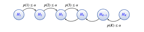
Figure 1: Graphical representation of Ordinal Prediction Interval (OPI) with $K$ nulls where $p(i)$ represents the conformal $p$-values.

3.3 Ordinal Prediction Set

Our second method for constructing ordinal prediction regions is based on Procedure 3. In this method, the prediction region $C(X_{2n+1})$ is defined simply using the acceptance region $A_{3}$ of Procedure 3, that is, $C(X_{2n+1})=\{y\in\mathcal{Y}:p(X_{2n+1},y)>\alpha\}$. Specifically, the prediction region consists of any class labels for which the corresponding hypotheses are not rejected by Procedure 3, resulting in a non-contiguous set of labels. This prediction region is referred to as a prediction set in this context. The procedure for constructing the prediction set is detailed in Algorithm 2 below.

Input: training set $\mathcal{D}_{train}=(X_{i},Y_{i})_{i=1}^{n}$, calibration set $\mathcal{D}_{cal}=(X_{i},Y_{i})_{i=n+1}^{2n}$, test observation $X_{2n+1}$, black-box algorithm $\mathcal{A}$, conformity score function $s$, mis-coverage level $\alpha.$

Output: Prediction set, $C(X_{2n+1}).$

Train a classifier $\mathcal{A}$ on $\mathcal{D}_{train}$;

for $(X_{i},Y_{i})\in\mathcal{D}_{cal}$ do

      Compute conformity score $s_{i}=s(X_{i},Y_{i})$;

end for

For each $y\in\mathcal{Y}$, compute conformity score $s_{2n+1}=s(X_{2n+1},y)$ and corresponding conformal $p$-value $p(X_{2n+1},y)$ using equation (1);

Prediction Set, $C(X_{2n+1})=\{y:p(X_{2n+1},y)>\alpha\}$.  

Algorithm 2 Ordinal Prediction Set

In the following, we present two results regarding the FWER control of Procedure 1-3 and (marginal) coverage guarantees of Algorithm 1-2 introduced as above.

Proposition 3.

Suppose that $(X_{i},Y_{i})_{i=n+1}^{2n+1}$ are exchangeable random variables, then Procedure 1-3 based on marginal conformal $p$-values, all strongly control the FWER at level $\alpha$, i.e., $FWER\leq\alpha$. Specifically, if the conformity scores $\{s_{i}\}_{i=n+1}^{2n+1}$ are distinct surely, then for Procedure 3, we also have, $FWER\geq\alpha-\frac{1}{n+1}.$

Theorem 1.

Suppose that $(X_{i},Y_{i})_{i=n+1}^{2n+1}$ are exchangeable random variables, then the prediction region $C(X_{2n+1})$ determined by Algorithm 1 and 2 both satisfy

$$\mathbb{P}(Y_{2n+1}\in C(X_{2n+1}))\geq 1-\alpha.$$

Specifically, for $C(X_{2n+1})$ determined by Algorithm 2, if the conformity scores $\{s_{i}\}_{i=n+1}^{2n+1}$ are distinct surely, we have

$$\mathbb{P}(Y_{2n+1}\in C(X_{2n+1}))\leq 1-\alpha+\frac{1}{n+1}.$$

3.4 Class-specific conditional coverage

To achieve more desired class-specific conditional coverage for our constructed prediction intervals and prediction sets, in Procedure 1-3 we use (class-specific) conditional conformal $p$-values $p(X_{2n+1}|y)$ as described in equation (3), instead of the marginal conformal $p$-values $p(X_{2n+1},y)$ for simultaneously testing $H_{1},\ldots,H_{K}$ formulated in equation (6). It is shown in Proposition 4 below that all these three modified procedures strongly control the conditional familywise error rate (FWER) at level $\alpha$, i.e., $\text{FWER}_{y}=\mathbb{P}(V>0|Y_{2n+1}=y)\leq\alpha$, for any $y\in\mathcal{Y}$, where $V$ is the number of type 1 errors. This result in turn leads to that the prediction regions $C(X_{n+1}|y)$ constructed by Algorithm 1 and 2 based on $p(X_{2n+1}|y)$ satisfy more desired (class-specific) conditional coverage, as stated in Theorem 2.

Proposition 4.

Under the same exchangeability assumption as in Proposition 2, Procedure 1-3 based on conditional conformal $p$-values $p(X_{2n+1}|y)$ all strongly control the conditional FWER at level $\alpha$, i.e., for any $y\in\mathcal{Y}$,

$$FWER_{y}=\mathbb{P}\{\textnormal{reject}~{}H_{y}|Y_{2n+1}=y\}\leq\alpha.$$

Specifically, if the conformity scores $\{s_{i}\}_{i\in\mathcal{I}_{y}\cup\{2n+1\}}$ are distinct surely, then for Procedure 3 based on $p(X_{2n+1}|y)$, we have that for any $y\in\mathcal{Y}$ and $\mathcal{I}_{y}\subseteq\mathcal{D}_{cal}$.

$$\mathbb{P}(\textnormal{reject}~{}H_{y}|Y_{2n+1}=y,\mathcal{I}_{y})\geq\alpha-\frac{1}{n_{y}+1}.$$

Theorem 2.

Under the same exchangeability assumption as in Theorem 1, the prediction region $C(X_{2n+1}|y)$ determined by Algorithm 1 or 2 based on conditional conformal $p$-values $p(X_{2n+1}|y)$ satisfies

$$\mathbb{P}\left(Y_{2n+1}\in C(X_{2n+1}|y)~{}\big{|}Y_{2n+1}=y\right)~{}\geq 1-\alpha$$

for any $y\in\mathcal{Y}$. Specifically, for the prediction set $C(X_{n+1}|y)$ determined by Algorithm 2 based on $p(X_{2n+1}|y)$, if the conformity scores $\{s_{i}\}_{i\in\mathcal{I}_{y}\cup\{2n+1\}}$ are distinct surely, we have

$$\mathbb{P}\left(Y_{2n+1}\in C(X_{2n+1}|y)~{}\big{|}Y_{n+1}=y,\mathcal{I}_{y}\right)\leq 1-\alpha+\frac{1}{n_{y}+1}$$

for any $y\in\mathcal{Y}$ and $\mathcal{I}_{y}\subseteq\mathcal{D}_{cal}$.

4 Numerical Study

In this section, we evaluate the performance of our four proposed methods, Ordinal Prediction Interval (OPI) in Algorithm 1 based on marginal conformal $p$-values (marginal OPI), the OPI based on conditional conformal $p$-values (conditional OPI), Ordinal Prediction Set (OPS) in Algorithm 2 based on marginal conformal $p$-values (marginal OPS), and the OPS based on conditional conformal $p$-values (conditional OPS), in comparison with the existing counterpart developed in Lu et al. (2022), Ordinal Adaptive Prediction Set (OAPS), on simulated data and one real dataset. The comparison is based on the marginal coverage, average set size, and class-specific conditional coverage of the prediction regions for a pre-specified level $\alpha$. The empirical metric we use to measure the class-specific conditional coverage (CCV) of the above methods is defined as

$$CCV=\max\limits_{y\in\{1,2,\cdots,K\}}\{(1-\alpha)-P_{y},0\},$$

where $P_{y}$ is the estimate of $\mathbb{P}(Y\in C(X_{2n+1}|y)~{}|Y=y)$ and $C(X_{2n+1}|y)$ is the prediction region obtained from Algorithm 1 or 2 using conditional conformal $p$-values for any $y\in\mathcal{Y}$. Intuitively, the metric measures the maximum of the deviance of the conditional coverage for each of the classes from the desired level of conditional coverage $1-\alpha$.

In the whole numerical investigations including simulation studies and real data analysis, we use the logistic regression algorithm as the black-box algorithm for our experiments and compute the conformity scores as estimated posterior probabilities of classes.

4.1 Simulations

We present the simulation study to evaluate the performance of our proposed methods along with the existing method. We consider two simulation settings below, a Gaussian mixture model and a sparse model.

1. Gaussian mixture. $(X|Y=k)\sim\pi_{1}N_{d}(\mu_{k},\Sigma)+\pi_{2}N_{d}(\mu_{k+1},\Sigma)$ for $k=1,2,3$ and $(X|Y=4)\sim\pi_{1}N(\mu_{4};\Sigma)+\pi_{2}N(\mu_{1};\Sigma)$ with $\pi_{1}=0.2,\pi_{2}=0.8$.

In the above setting, we set $d=2$, $\mu_{1}=(-1,0)$, $\mu_{2}=(-1,-1)$, $\mu_{3}=(0,-1)$, $\mu_{4}=(1,-1)$, and $\Sigma$ as the equal correlation matrix with correlation $=0.1$.

2. Sparse model. The sparse model is generated with different dimensions of feature vector with $d=5,10,20,50,\text{ or }100$. The features are generated with $X_{i}\sim N(0,1)$ with $Cov(X_{i},X_{j})=0.5$ for $i\neq j.$ The class labels are generated using the sigmoid function $f(x)$ and the the following decision rule,

$$Y_{i}=k\hskip 11.38109ptif\hskip 11.38109pt\frac{k-1}{4}\leq f(x_{i})<\frac{k}{4},\hskip 5.69054ptwhere\hskip 5.69054ptk=1,2,3,4,$$

where $f(x)={1}/{(1+e^{-\beta^{{}^{\prime}}x})}$ with $\beta=(\beta_{1},\cdots,\beta_{d})^{\prime}$ and $x=(x_{1},\ldots,x_{d})^{\prime}$. The value of $\beta$ is set as $(\beta_{1},\ldots,\beta_{5})=(1,1,1,-\sqrt{2},1)$, and $\beta_{i}=0$ for any $5<i\leq d$.

The sample size for these two simulation settings is 2,000, out of which 500 samples have been used to train the classifier, 525 observations for calibration, and 975 for validation. The simulations are repeated 500 times, and the results are averaged to obtain the final performance metrics.

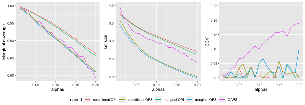
Figure 2: Performance comparison of four proposed methods OPS and OPI using marginal and conditional conformal $p$-values with the existing Ordinal APS under simulation setting 1 in terms of marginal coverage (left), average set size (middle) and class-specific conditional coverage (right) of the prediction sets.

Figure 2 displays the performance of our proposed methods along with the existing method under simulation setting 1. It can be seen from the left panel of Figure 2 that all these five methods empirically achieve the desired level of marginal coverage. The middle panel of Figure 2 compares the set sizes of the prediction regions corresponding to these five methods. It can be seen from the figure that the marginal OPS and the conditional OPS use shorter set sizes to attain the proper marginal coverage than the existing OAPS whereas the OAPS has shorter set sizes than the marginal OPI and the conditional OPI. Finally, while the marginal coverage is guaranteed by all the methods, the right panel of Figure 2 shows their differences in class-specific conditional coverage; the existing OAPS exhibits the largest value of CCV compared to the proposed methods and among the four proposed methods, the conditional OPI and conditional OPS exhibit lower values of CCV than the marginal OPI and marginal OPS.

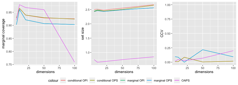
Figure 3: Performance comparison of four proposed methods with existing Ordinal APS under simulation setting 2 with different dimensions of inputs and fixed mis-coverage level $\alpha=0.1$ in terms of marginal coverage (left), average set size (middle) and CCV (right) of the prediction sets.

Figure 3 shows the performance of our proposed methods along with the existing method under simulation setting 2 with different dimensions of inputs. It can be seen from the left panel of this figure that all these methods empirically achieve desired marginal coverage for lower dimensions, however, the existing OAPS massively undercovers for higher dimensions and thus loses the control of mis-coverage rate. From the middle and right panels of Figure 3, we can also see that the conditional OPI and conditional OPS achieve lower values of CCV than the existing OAPS, although the OAPS has the lower set sizes than our proposed methods for various dimensions of input.

4.2 Application to real data

We also evaluate the performance of our proposed methods on a real dataset, Traffic accident data, which is publicly available on the website of Leeds City Council. The real data consists of 1,908 traffic accidents that occurred in the year 2019. The objective is to predict the severity of the casualties, which are classified into three categories – mild, serious, and fatal based on the features available. In the numerical experiment, 500 observations are used to train the logistic regression model, $35\%$ of the remaining observations are used for calibration, and $65\%$ for validation. Figure 4 shows that all these methods empirically achieve desired marginal coverage for different levels of mis-coverage, however, the proposed marginal OPI and marginal OPS, and existing OAPS have lower set sizes than the conditional OPI and conditional OPS. It is also evident from Figure 4 that the proposed conditional OPS and conditional OPI both attain desired class-specific conditional coverage unlike the existing method, OAPS, which seems to largely deviate from the desired level of conditional coverage.

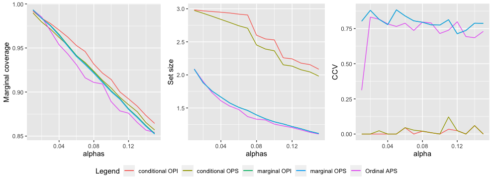
Figure 4: Performance comparison of four proposed methods OPS and OPI using marginal and conditional conformal $p$-values with the existing Ordinal APS in terms of marginal coverage (left), average set size (middle) and CCV (right) of the prediction regions for Traffic Accident Data.

5 Concluding Remarks

In this paper, we discussed the ordinal classification problem in the framework of conformal prediction and introduced two types of conformal methods, OPI and OPS, for constructing distribution-free contiguous prediction regions and non-contiguous prediction sets, respectively. These methods are developed by leveraging the idea of multiple testing with the FWER control and are specifically designed based on marginal conformal $p$-values and (class-specific) conditional conformal $p$-values, respectively. Theoretically, it was proved that the proposed methods based on marginal and conditional $p$-values respectively achieve satisfactory levels of marginal and class-specific conditional coverages. Through some numerical investigations including simulations and real data analysis, our proposed methods show promising results for the settings of higher dimensions and for class-specific conditional coverage.

This paper discussed constructing valid prediction set for single test input. It would be interesting to discuss how to construct (simultaneous) prediction sets for multiple test inputs with some overall error control such as false discovery rate (FDR) control. Another interesting extension might be to relax the conventional distributional assumption we used for classification problems, for which the training data and the test data follow from the same distribution. It will be interesting to see whether the proposed methods can be extended to the settings of distribution shift where the training and test data sets have different distributions.

Appendix A Proofs

A.1 Proof of Proposition 1

Proof.

Suppose, for any given values of conformity scores, $v_{1},\cdots,v_{n+1},$ they can be rearranged as $\tilde{v}_{1}<\cdots<\tilde{v}_{k}$ with repetitions $n_{i}$ of $\tilde{v}_{i}$ such that $\sum_{i=1}^{k}n_{i}=n+1$. Let $E_{v}$ denote the event of $\{s_{n+1},\cdots,s_{2n+1}\}=\{v_{1},\cdots,v_{n+1}\}$. Then, under $E_{v}$, for $i=1,\cdots,k$, we have

$$\mathbb{P}(s_{2n+1}=\tilde{v}_{i}|E_{v})=\frac{n_{i}}{n+1},$$

due to the exchangeability of $s_{i}$’s,

We also note that under $E_{v}$ and $s_{2n+1}=\tilde{v}_{i}$ we have from equation (5),

$$p(Z_{2n+1})=\frac{\sum_{l=1}^{i}n_{l}}{n+1}.$$ (7)

Then, for any $t\in[0,1]$ and $i=1,\cdots,k$, we have

$$\mathbb{P}(p(Z_{2n+1})\leq t|E_{v},s_{2n+1}=\tilde{v}_{i})=\begin{cases}0&\text{if }t<\frac{\sum_{l=1}^{i}n_{l}}{n+1},\\ 1&\text{o.w.}\end{cases}$$ (8)

Thus, for any $i=1,\cdots,k$ and $\frac{\sum_{l=1}^{i-1}n_{l}}{n+1}\leq t<\frac{\sum_{l=1}^{i}n_{l}}{n+1}$, we have

$$\qquad\mathbb{P}(p(Z_{2n+1})\leq t|E_{v})$$

$$=\sum_{l=1}^{k}\mathbb{P}(p(Z_{2n+1})\leq t|E_{v},s_{2n+1}=\tilde{v}_{l})\cdot\mathbb{P}(s_{2n+1}=\tilde{v}_{l}|E_{v})$$

$$=\frac{\sum_{l=1}^{i-1}n_{l}}{n+1}\leq t.$$

By taking the expectation on the above inequality, it follows that the conformal $p$-value $p(Z_{2n+1})$ is marginally valid.

Specifically, if conformity scores $\{s_{i}\}_{i=n+1}^{2n+1}$ are distinct surely, then $k=n+1$ and $n_{i}=1$ for $i=1,\ldots,n+1$. Thus,

$\mathbb{P}\left(p(Z_{2n+1})\leq t|E_{v}\right)=\frac{i-1}{n+1},\textnormal{ if }\frac{i-1}{n+1}\leq t<\frac{i}{n+1},$

that is,

$$p(Z_{2n+1})|E_{v}\sim U\Bigl{\{}\frac{1}{n+1},\cdots,1\Bigl{\}}.$$

This completes the proof. ∎

A.2 Proof of Proposition 2

Proof.

For any given $y\in\mathcal{Y}$, the corresponding (class-specific) conditional conformal $p$-value is given by

$$p(X_{2n+1}|y)=\frac{1}{n_{y}+1}\left[\sum_{i\in\mathcal{I}_{y}}\mathbb{I}\{s_{i}\leq s_{2n+1}\}+1\right],$$ (9)

where $\mathcal{I}_{y}=\{i:(X_{i},Y_{i})\in\mathcal{D}_{cal},Y_{i}=y\}$, $n_{y}=|\mathcal{I}_{y}|$, $s_{i}=s(X_{i},y)$ for $i\in\mathcal{I}_{y}$, and $s_{2n+1}=s(X_{2n+1},y)$. Given $I_{y}$ and $Y_{2n+1}=y$, $(X_{i})_{i\in\mathcal{I}_{y}}\cup\{X_{2n+1}\}$ are exchangeably distributed, which is due to the assumption that $(X_{i},Y_{i})_{i=1}^{2n+1}$ are exchangeably distributed. Using the similar arguments as in the proof of Proposition 1, for any given values of $v_{1},\cdots,v_{n_{y}+1}$, suppose that they can be arranged as $\tilde{v}_{1}<\cdots<\tilde{v}_{l}$ with repetitions $m_{i}$ of $\tilde{v}_{i}$ such that $\sum_{i=1}^{l}m_{i}=n_{y}+1$.

Let $E_{v}$ denote the event $\{s_{i}\}_{i\in\mathcal{I}_{y}}\cup\{s_{2n+1}\}=\{v_{1},\cdots,v_{n_{y}+1}\}$. Then, given $E_{v},I_{y}$, and $Y_{2n+1}=y$, we have

$$\mathbb{P}(s_{2n+1}=\tilde{v}_{i}|E_{v},I_{y},Y_{2n+1}=y)=\frac{m_{i}}{n_{y}+1}$$

for $i=1,\cdots,l$ and $y=1,\cdots,K$, due to exchangeability of $s_{i}$, $i\in I_{y}\cup\{2n+1\}$ given $I_{y}$, which in turn is due to exchangeability of $(X_{i},Y_{i})_{i=1}^{2n+1}$. Note that given $E_{v}$, $I_{y}$, $Y_{2n+1}=y$, and $s_{2n+1}=\tilde{v}_{i}$, we have from equation (9),

$$p(X_{2n+1}|y)=\frac{\sum_{j=1}^{i}m_{j}}{n_{y}+1}.$$

Thus, for any $t\in[0,1]$ and $i=1,\cdots,l$,

$$\mathbb{P}\left(p(X_{2n+1}|y)\leq t\big{|}E_{v},I_{y},Y_{2n+1}=y,s_{2n+1}=\tilde{v}_{i}\right)=\begin{cases}0&\text{if }t<\frac{\sum_{j=1}^{i}m_{j}}{n_{y}+1},\\ 1&\text{o.w.}\end{cases}$$ (10)

Then, for any given $i=1,\cdots,l$ and $\frac{\sum_{j=1}^{i}m_{j}}{n_{y}+1}\leq t<\frac{\sum_{j=1}^{i+1}m_{j}}{n_{y}+1}$, we have

$$\qquad\mathbb{P}\left(p(X_{2n+1}|y)\leq t\big{|}E_{v},I_{y},Y_{2n+1}=y\right)$$

$$=\sum_{j=1}^{l}\mathbb{P}\left(p(X_{2n+1}|y)\leq t\big{|}E_{v},I_{y},Y_{2n+1}=y,s_{2n+1}=\tilde{v}_{i}\right)\cdot\mathbb{P}\left(s_{2n+1}=\tilde{v}_{i}\big{|}E_{v},I_{y},Y_{2n+1}=y\right)$$

$$=\frac{\sum_{j=1}^{i}m_{j}}{n_{y}+1}\leq t.$$

By taking expectation, it follows that $p(X_{2n+1}|y)$ is conditionally valid given $Y_{2n+1}=y$. ∎

A.3 Proof of Proposition 3

Proof.

Consider Procedure 1-3 based on marginal conformal $p$-values. Note that among the tested hypotheses $H_{1},\ldots,H_{K}$, there is exactly one hypothesis $H_{Y_{2n+1}}$ to be true. Thus, the FWER of Procedure 1-3 are all equal to

$$\mathbb{P}(\text{reject }H_{Y_{2n+1}})\leq\mathbb{P}\left(p(X_{2n+1},Y_{2n+1})\leq\alpha\right)\leq\alpha,$$

where the last inequality follows by Proposition 1.

Specifically, for Procedure 3, if the conformity scores $\{s_{i}\}_{i=n+1}^{2n+1}$ are distinct surely, by Proposition 1, we have

$$\qquad\text{FWER}=\mathbb{P}(\text{reject }H_{Y_{2n+1}})=\mathbb{P}\Bigl{\{}p(X_{2n+1},Y_{2n+1})\leq\alpha\Bigl{\}}~{}\geq\alpha-\frac{1}{n+1},$$

the desired result. ∎

A.4 Proof of Theorem 1

Proof.

Note that the prediction set derived from Algorithm 1 is given by $C(X_{2n+1})=A_{1}\cap A_{2}.$ Thus, by Proposition 1,

$$\mathbb{P}(Y_{2n+1}\in C(X_{2n+1}))\geq\mathbb{P}(p(X_{2n+1}),Y_{2n+1})>\alpha)\geq 1-\alpha.$$

Similarly, for Algorithm 2, its prediction set is given by $C(X_{2n+1})=\{y\in\mathcal{Y}:p(X_{2n+1},y)>\alpha\}.$ By Proposition 1, it is easy to check that

$$\mathbb{P}(Y_{2n+1}\in C(X_{2n+1}))=\mathbb{P}(p(X_{2n+1},Y_{2n+1})>\alpha)\geq 1-\alpha.$$

Specifically, if the conformity scores $\{s_{i}\}_{i=1}^{2n+1}$ are distinct surely, for Algorithm 2, we have

$$\mathbb{P}(Y_{2n+1}\in C(X_{2n+1}))=1-\mathbb{P}(p(X_{2n+1},Y_{2n+1})\leq\alpha)\leq 1-\alpha+\frac{1}{n+1}.$$

This completes the proof. ∎

A.5 Proof of Proposition 4

Proof.

Consider Procedure 1-3 based on conditional conformal $p$-values. For any $y=1,\cdots,K$, given $Y_{2n+1}=y$, the conditional FWER of Procedure 1-3 are all equal to

$$\mathbb{P}(\text{reject }H_{y}|Y_{2n+1}=y)\leq\mathbb{P}(p(X_{2n+1}|y)\leq\alpha|Y_{2n+1}=y)\leq\alpha,$$

where the inequalities follow the definitions of Procedure 1-3 and Proposition 2.

Specifically, for Procedure 3, if the conformity scores $\{s_{i}\}_{i\in\mathcal{I}_{y}\cup\{2n+1\}}$ are distinct surely, then by Proposition 2, the FWER conditional on $I_{y}$ and $Y_{2n+1}=y$ is equal to

$$\mathbb{P}\Bigl{\{}\text{reject}~{}H_{y}~{}\big{|}I_{y},Y_{2n+1}=y\Bigl{\}}=\mathbb{P}(p(X_{2n+1}|y)\leq\alpha|I_{y},Y_{2n+1}=y)\geq\alpha-\frac{1}{n_{y}+1}.$$

This completes the proof. ∎

A.6 Proof of Theorem 2

Proof.

By using Proposition 4 and the similar arguments as in the proof of Theorem 1, the prediction sets $C(X_{2n+1}|y)$ derived from Algorithm 1 and 2 based on the conditional conformal $p$-values $p(X_{2n+1}|y)$ all satisfy,

$$\mathbb{P}\Bigl{\{}Y_{2n+1}\in C(X_{2n+1}|y)~{}\big{|}I_{y},Y_{2n+1}=y\Bigl{\}}~{}\geq 1-\alpha$$

for any $y=1,\ldots,K$. Specifically, if the conformity scores $\{s_{i}\}_{i\in\mathcal{I}_{y}\cup\{2n+1\}}$ are distinct surely, for Algorithm 2, we have

$$\mathbb{P}\Bigl{\{}Y_{2n+1}\in C(X_{2n+1}|y)~{}\big{|}I_{y},Y_{2n+1}=y\Bigl{\}} =\mathbb{P}\Bigl{\{}p(X_{2n+1}|y)>\alpha~{}\big{|}I_{y},Y_{2n+1}=y\Bigl{\}}$$

$$\leq 1-\alpha+\frac{1}{n_{y}+1},$$

the desired result. ∎

References

- Agresti (2010) Alan Agresti. Analysis of ordinal categorical data. John Wiley & Sons, 2010.
- Angelopoulos and Bates (2021) A.N. Angelopoulos and S. Bates. A gentle introduction to conformal prediction and distribution-free uncertainty quantification. arXiv preprint arXiv:2107.07511, 2021.
- Angelopoulos et al. (2020) Anastasios Angelopoulos, Stephen Bates, Jitendra Malik, and Michael I. Jordan. Uncertainty sets for image classifiers using conformal prediction. arXiv preprint arXiv:2009.14193, 2020.
- Barber et al. (2021) Rina Foygel Barber, Emmanuel J Candes, Aaditya Ramdas, and Ryan J Tibshirani. The limits of distribution-free conditional predictive inference. Information and Inference: A Journal of the IMA, 10(2):455–482, 2021.
- Cardoso and da Costa (2007) Jaime Cardoso and Joaquim Pinto da Costa. Learning to classify ordinal data: The data replication method. Journal of Machine Learning Research, 8:1393–1429, 2007.
- Cauchois et al. (2021) Maxime Cauchois, Suyash Gupta, and John C Duchi. Knowing what you know: valid and validated confidence sets in multiclass and multilabel prediction. The Journal of Machine Learning Research, 22(1):3681–3722, 2021.
- Cheng et al. (2008) Jianlin Cheng, Zheng Wang, and Gianluca Pollastri. A neural network approach to ordinal regression. In 2008 IEEE International Joint Conference on Neural Networks, pages 1279–1284. IEEE, 2008.
- da Costa et al. (2010) Joaquim F Pinto da Costa, Ricardo Sousa, and Jaime S Cardoso. An all-at-once unimodal svm approach for ordinal classification. In 2010 Ninth International Conference on Machine Learning and Applications, pages 59–64. IEEE, 2010.
- Dmitrienko et al. (2009) Alex Dmitrienko, Ajit C Tamhane, and Frank Bretz. Multiple testing problems in pharmaceutical statistics. CRC press, 2009.
- Fontana et al. (2023) Matteo Fontana, Gianluca Zeni, and Simone Vantini. Conformal prediction: a unified review of theory and new challenges. Bernoulli, 29(1):1–23, 2023.
- Frank and Hall (2001) Eibe Frank and Mark Hall. A simple approach to ordinal classification. In 12th European Conference on Machine Learning, Proceedings 12, pages 145–156. Springer, 2001.
- Gibbs and Candes (2021) Isaac Gibbs and Emmanuel Candes. Adaptive conformal inference under distribution shift. Advances in Neural Information Processing Systems, 34:1660–1672, 2021.
- Gutiérrez et al. (2015) Pedro Antonio Gutiérrez, Maria Perez-Ortiz, Javier Sanchez-Monedero, Francisco Fernandez-Navarro, and Cesar Hervas-Martinez. Ordinal regression methods: survey and experimental study. IEEE Transactions on Knowledge and Data Engineering, 28(1):127–146, 2015.
- Harrell (2015) Frank E Harrell. Ordinal logistic regression. In Regression modeling strategies: with applications to linear models, logistic and ordinal regression, and survival analysis, pages 311–325. Springer, 2015.
- Hechtlinger et al. (2018) Yotam Hechtlinger, Barnabás Póczos, and Larry Wasserman. Cautious deep learning. arXiv preprint arXiv:1805.09460, 2018.
- Hüllermeier and Waegeman (2021) Eyke Hüllermeier and Willem Waegeman. Aleatoric and epistemic uncertainty in machine learning: an introduction to concepts and methods. Machine Learning, 110:457–506, 2021.
- Janitza et al. (2016) Silke Janitza, Gerhard Tutz, and Anne-Laure Boulesteix. Random forest for ordinal responses: prediction and variable selection. Computational Statistics & Data Analysis, 96:57–73, 2016.
- Kramer et al. (2001) Stefan Kramer, Gerhard Widmer, Bernhard Pfahringer, and Michael De Groeve. Prediction of ordinal classes using regression trees. Fundamenta Informaticae, 47(1-2):1–13, 2001.
- Lei (2014) J. Lei. Classification with confidence. Biometrika, 101(4):755–769, 2014.
- Lu et al. (2022) C. Lu, A.N. Angelopoulos, and S. Pomerantz. Improving trustworthiness of ai disease rating in medical imaging with ordinal conformal prediction sets. arXiv preprint arXiv:2207.02238, 2022.
- McCullagh (1980) Peter McCullagh. Regression models for ordinal data. Journal of the Royal Statistical Society B, 42:109–142, 1980.
- Papadopoulos et al. (2002) Harris Papadopoulos, Kostas Proedrou, Volodya Vovk, and Alex Gammerman. Inductive confidence machines for regression. In 13th European Conference on Machine Learning, Proceedings 13, pages 345–356. Springer, 2002.
- Rifkin and Klautau (2004) Ryan Rifkin and Aldebaro Klautau. In defense of one-vs-all classification. The Journal of Machine Learning Research, 5:101–141, 2004.
- Romano et al. (2020) Y. Romano, M. Sesia, and E. Candès. Classification with valid and adaptive coverage. In Advances in Neural Information Processing Systems, volume 33, pages 3581–3591, 2020.
- Sadinle et al. (2019) M. Sadinle, J. Lei, and L. Wasserman. Least ambiguous set-valued classifiers with bounded error levels. Journal of American Statistical Association, 114:223–234, 2019.
- Shafer and Vovk (2008) G. Shafer and V. Vovk. A tutorial on conformal prediction. Journal of Machine Learning Research, 9:371–421, 2008.
- Tibshirani et al. (2019) Ryan J Tibshirani, Rina Foygel Barber, Emmanuel Candes, and Aaditya Ramdas. Conformal prediction under covariate shift. Advances in Neural Information Processing Systems, 32, 2019.
- Tyagi and Guo (2023) Chhavi Tyagi and Wenge Guo. Multi-label classification under uncertainty: a tree-based conformal prediction approach. In Conformal and Probabilistic Prediction with Applications, pages 488–512. PMLR, 2023.
- Vovk et al. (2005) V. Vovk, A. Gammerman, and G. Shafer. Algorithmic learning in a random world. Springer, 2005.
- Vovk (2012) Vladimir Vovk. Conditional validity of inductive conformal predictors. In Asian Conference on Machine Learning, pages 475–490. PMLR, 2012.
- Vovk et al. (1999) Vladimir Vovk, Alex Gammerman, and Craig Saunders. Machine-learning applications of algorithmic randomness. In Sixteenth International Conference on Machine Learning, pages 444–453, 1999.
- Xu et al. (2023) Yunpeng Xu, Wenge Guo, and Zhi Wei. Conformal risk control for ordinal classification. In Uncertainty in Artificial Intelligence, pages 2346–2355. PMLR, 2023.