Waveform systematics in gravitational-wave inference of signals from binary neutron star merger models incorporating higher order modes information
Abstract
Accurate information from gravitational wave signals from coalescing binary neutron stars provides essential input to downstream interpretations, including inference of the neutron star population and equation of state. However, even adopting the currently most accurate and physically motivated models available for parameter estimation (PE) of BNSs, these models remain subject to waveform modeling uncertainty: differences between these models may introduce biases in recovered source properties. In this work, we describe injection studies investigating these systematic differences between the two best waveform models available for BNS currently, NRHybSur3dq8Tidal and TEOBResumS. We demonstrate that for BNS sources observable by current second-generation detectors, differences for low-amplitude signals are significant for certain sources.
I Introduction
Since the discovery of gravitational waves from GW150914 Abbott et al. (2016) (The LIGO Scientific Collaboration and the Virgo Collaboration), the Advanced Laser Interferometer Gravitational-Wave Observatory (LIGO) LIGO Scientific Collaboration et al. (2015) and Virgo Accadia and et al (2012); Acernese et al. (2015) detectors continue to discover gravitational waves (GW) from coalescing binary black holes (BBHs) and neutron stars. The properties of each source are inferred by comparing each observation to some estimate(s), commonly called an approximant, for the GWs emitted when a BBH merges. As illustrated recently with GW190521 The LIGO Scientific Collaboration et al. (2020a, b), GW190814 The LIGO Scientific Collaboration et al. (2020c), GW190412 The LIGO Scientific Collaboration et al. (2020d), and the discussion in GWTC-3 Abbott et al. (2021a), these approximations have enough differences with respect to to each other to produce noticeable differences in inferred posterior distributions, consistent with prior work Shaik et al. (2019); Williamson et al. (2017); Pürrer and Haster (2020). Despite ongoing generation of new waveforms with increased accuracy Hannam et al. (2014); Khan et al. (2019); Bohé et al. (2017); Varma et al. (2019); Pratten et al. (2020); Ossokine et al. (2020), these previous investigations suggest that waveform model systematics can remain a limiting factor in inferences about individual events Shaik et al. (2019) and populations Wysocki et al. (2019a); Pürrer and Haster (2020).
Waveform systematics could be particularly pernicious for detailed analyses to infer the nuclear equation of state from GW observations. For analyses not involving postmerger physics, these approaches look for the subtle impact of matter on the pre-merger inspiral radiation, due to tidal deformations and altered inspiral rate Gamba et al. (2021); Narikawa and Uchikata (2022); Chatziioannou (2022); Kunert et al. (2022); Ashton and Dietrich (2021); Riemenschneider et al. (2021). Even though the GW signal from the early inspiral is well understood because tidal effects are small and accumulate only at the very end of the inspiral, they’re embedded deep within the most challenging strong field component of the GW signal. One known limitation of most previous investigations of waveform systematics for BNS is the neglect of higher-order modes (HOM). Current state-of-the-art BNS models TEOBResumS Nagar et al. (2018) and NRHybSur3dq8Tidal Barkett et al. (2020) incorporate higher-order-modes enabling the exploration of these effects. For example, GW190412 The LIGO Scientific Collaboration et al. (2020d), which was a merger of two black holes that were highly asymmetric in masses, 30 and 8, demonstrated the existence and importance of HOM in parameter inference of GW from binary mergers Islam et al. (2021). Using models that incorporate HOM can significantly impact the inferred parameters of sources identified with current-generation instruments for GW170817 or GW170817-like signals, as demonstrated in Lange et al. (2022); Calderón Bustillo et al. (2021). Despite their expected significance to parameter inference, most studies of BNS systematics omit them and rarely perform large-scale parameter inference studies to fully assess the impact of systematics, although a similar study was done in Huang et al. (2021). For example, several mismatch studies are mostly done for models having only leading-order (2,2) mode Samajdar and Dietrich (2018, 2019); Dietrich et al. (2021). A study done with fiducial BNS signals with HOMs argued that biases in inferring the reduced tidal parameter could be larger than the statistical 90 only for very high SNR signals 80 Gamba et al. (2021) in the LIGO-Virgo band. Recent work by Narikawa Narikawa (2023) looked at the effects of multipoles by comparing MultipoleTidal model to PNTidal and NRTidalv2 waveforms, showing that mismatches and phases do differ between them for systems with higher mass and large tidal deformabilities.
This paper is organized as follows. In Section II, we review the use of RIFT for parameter inference; the waveform models used in this work; and the techniques used in Jan et al. (2020) to assess systematic error. We describe one fiducial ensembles of synthetic sources, targeted at the most common (low) amplitude sources. In Section III, we use two well-studied waveform models to demonstrate the impact of contemporary model systematics. We show that model systematics will be important, at a level which must impact population results and consistency tests like PP plots. In Section IV, we summarize our results and discuss their potential applications to future GW sources and population inference.
II Methods
II.1 RIFT review
A coalescing compact binary in a quasi-circular orbit can be completely characterized by its intrinsic and extrinsic parameters. By intrinsic parameters, we refer to the binary’s detector-frame masses , spins , and any quantities characterizing matter in the system, . By extrinsic parameters, we refer to the seven numbers needed to characterize its spacetime location and orientation; luminosity distance (), right ascension (), declination (), inclination (), polarization (), coalescence phase (), and time (). We will express masses in solar mass units and dimensionless nonprecessing spins in terms of cartesian components aligned with the orbital angular momentum , as we use waveform models that do not account for precession. We will use , to refer to intrinsic and extrinsic parameters, respectively.
RIFT Lange et al. (2018); Wofford et al. (2023) consists of a two-stage iterative process to interpret gravitational wave data via comparison to predicted gravitational wave signals . In one stage, for each from some proposed “grid” of candidate parameters, RIFT computes a marginal likelihood
| (1) |
from the likelihood of the gravitational wave signal in the multi-detector network, accounting for detector response; see the RIFT paper for a more detailed specification Lange et al. (2018); Wofford et al. (2023). In the second stage, RIFT performs two tasks. First, it generates an approximation to based on its accumulated archived knowledge of marginal likelihood evaluations . This approximation can be generated by Gaussian processes, random forests, or other suitable approximation techniques. Second, using this approximation, it generates the (detector-frame) posterior distribution
| (2) |
where prior is prior on intrinsic parameters like mass and spin. The posterior is produced by performing a Monte Carlo integral: the evaluation points and weights in that integral are weighted posterior samples, which are fairly resampled to generate conventional independent, identically distributed “posterior samples.” For further details on RIFT’s technical underpinnings and performance, see Lange et al. (2018); Wofford et al. (2023); Wysocki et al. (2019b); Lange (2020).
II.2 Waveform models
The tidal waveform models used in this study are IMRPhenomD_NRTidalv2, NRHybSur3dq8Tidal, and TEOBResumS. NRTidalv2 models Dietrich et al. (2019) are improved versions of NRTidal Dietrich et al. (2017) models, which are closed-form tidal approximants for binary neutron star coalescence and have been analytically added to selected binary black hole GW model to obtain a binary neutron star waveform, either in the time or in the frequency domain. The NRHybSur3dq8Tidal Barkett et al. (2020) tidal model is based on the binary black hole hybrid model NRHybSur3dq8, which is constructed via an interpolation of NR waveforms. It includes all modes , () but not () and (4,0) and models tidal effect up to . This model combines the accuracy of surrogate waveforms with the efficiency of PN models. TEOBResumS Nagar et al. (2018) is another but unique time-domain EOB formalism that includes tidal effects for all modes , but no and models tidal effect up to and for spins up to 0.5.
II.3 Fiducial synthetic sources and PP tests
We consider one universe of 100 synthetic signals for a 3-detector network (HLV), with masses drawn uniformly in in the region bounded by , and for each object uniformly distributed up to 1000. These bounds are expressed in terms of and , and encompass the detector-frame parameters of neutron stars observed till date The LIGO Scientific Collaboration et al. (2017); Abbott et al. (2020); Abbott et al. (2021b). The extrinsic parameters are drawn uniformly in sky position and isotropically in Euler angles, with source luminosity distances drawn proportional to between and for low SNR injections. All our sources have non-precessing spins, with each component assumed to be uniform between , this is due to limitations of the NRHybSur3dq8Tidal model.
For complete reproducibility, we use NRHybSur3dq8Tidal, TEOBResumS and IMRPhenomD_NRTidalv2, starting the signal evolution and likelihood integration at , performing all analysis with time series in Gaussian noise with known advanced LIGO design PSDs LIGO Scientific Collaboration (2018). The BNS signal is generated for 300 seconds but analysis was performed only on 128 seconds of data. For each synthetic event and interferometer, we use the same noise realization for all waveform approximations. Therefore, the differences between them arise solely due to waveform systematics. The NRHybSur3dq8Tidal model is utilized with two settings: a) and b) , which includes only the dominant quadrupole mode. TEOBResumS and IMRPhenomD_NRTidalv2 approximants are used with and settings respectively.
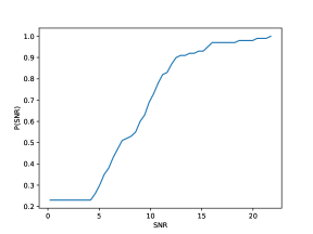
Fig. 1 shows the cumulative SNR distribution (under a “zero-noise” assumption) of the specific synthetic population generated from this distribution. Compared to GW170817’s confident detection, which was a BNS merger that occurred at detected by LIGO-Virgo with a SNR of 32.4, the majority of the signals in this fiducial population have SNRs below or near the typical detection criteria for a BNS merger, with some having high enough amplitudes.
By using a very modest-amplitude population to assess the impact of waveform systematics, we demonstrate their immediate impact on the kinds of analyses currently being performed on real observations, let alone future studies.
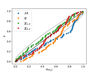
One way to assess the performance of parameter inference is a probability-probability plots (usually denoted PP-plot) Cook et al. (2006). Using RIFT on each source , with true parameters , we estimate the fraction of the posterior distributions which is below the true source value [] for each intrinsic parameter . After reindexing the sources so increases with for some fixed , the panels of Figure 5 for example, show a plot of versus for all binary parameters for different scenarios.
| Injection model | Recovery model |
|---|---|
| NRHybSur3dq8Tidal() | NRHybSur3dq8Tidal() |
| NRHybSur3dq8Tidal() | NRHybSur3dq8Tidal() |
| NRHybSur3dq8Tidal() | TEOBResumS() |
| NRHybSur3dq8Tidal() | IMRPhenomD_NRTidalv2 |
| NRHybSur3dq8Tidal() | IMRPhenomD |
| TEOBResumS() | TEOBResumS() |
| TEOBResumS() | NRHybSur3dq8Tidal() |
| TEOBResumS() | IMRPhenomD_NRTidalv2 |
| TEOBResumS() | IMRPhenomD |
II.4 JS test
To more sharply identify subtle differences introduced by waveform systematics, we will directly compare pairs of inferred posterior probability distributions deduced with different waveforms but from the same set of data to each other. Many pairwise error diagnostics have been used in the literature in general and with RIFT, in particular, Wofford et al. (2023). In this study, motivated by previous work Ashton and Talbot (2021), we use the one-dimensional Jensen-Shannon (JS) divergence where and . The JS divergence is symmetric, ranges between 0 (for identical distributions) and 1. For the multidimensional problems described here, we adopt the median JS divergence over all parameters. Analyses of O3 using multiple waveforms suggest that binary black holes analyzed with different contemporary waveforms will produce answers differing by The LIGO Scientific Collaboration et al. (2019); Abbott et al. (2021); Islam et al. (2023).
III Results
Our investigations corroborate our central expectation: inferences computed with different waveforms are frequently substantially different, even for BNS and even for near-threshold events. The most extreme contrast appeared between TEOBResumS and other waveform models, where for our near-threshold synthetic events we found ubiquitous qualitatively different inferences.
III.1 Anecdotal examples
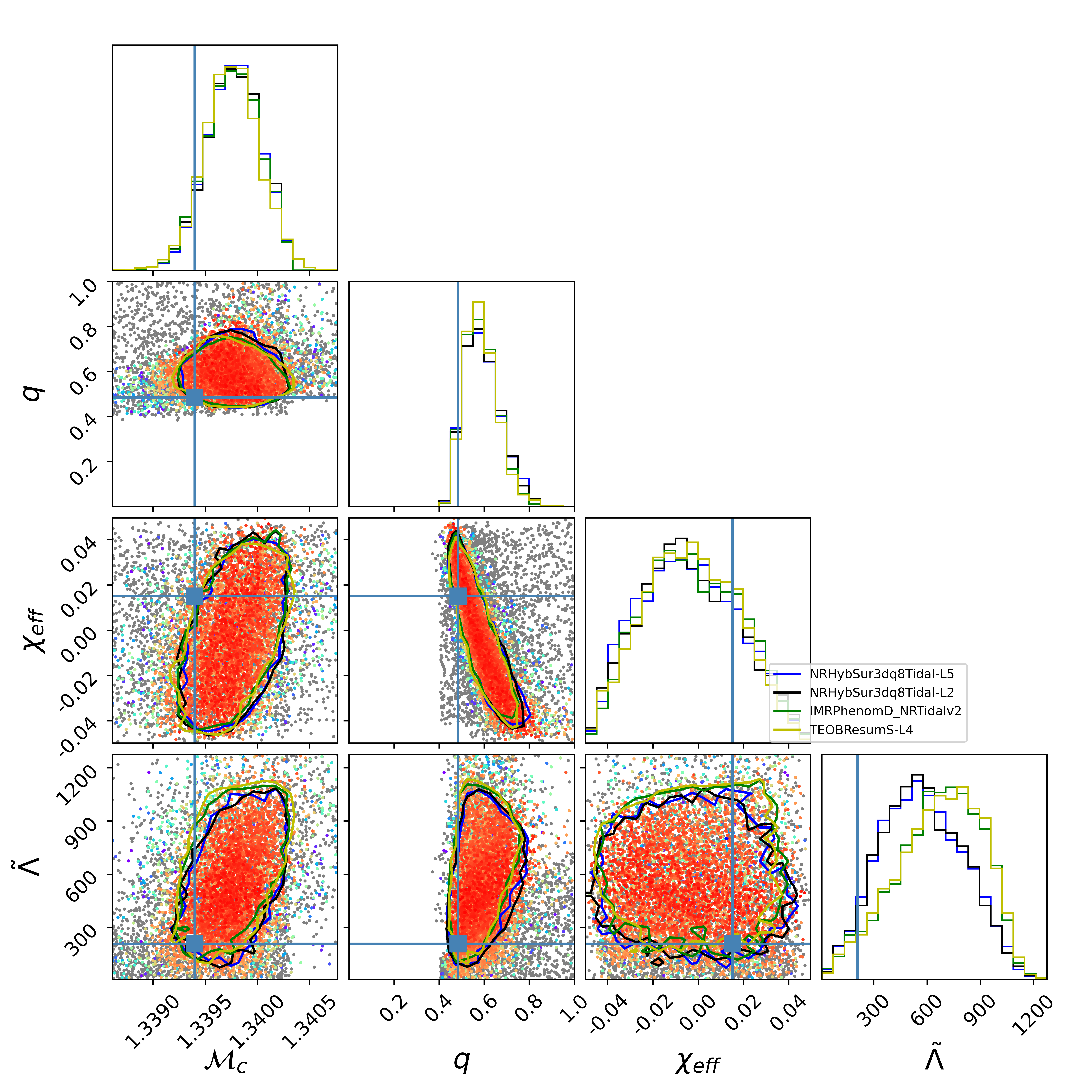
As an illustrative example of the systematics explored more comprehensively in the population studies below, Figure 2 shows the results of parameter inference using multiple recovery waveforms applied to the same synthetic data source, here a low-amplitude NRHybSur3dq8Tidal-lmax5 injection. Despite its low signal amplitude, this example shows that posterior distributions derived from the same synthetic data will differ, depending on the GW signal model used to interpret it.
III.2 JS divergences: Demonstrating and quantifying waveform systematics
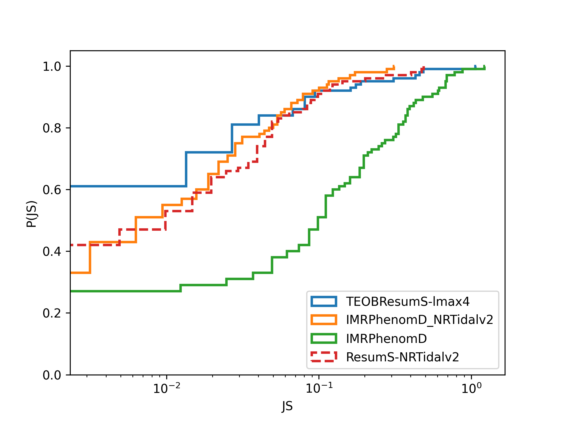
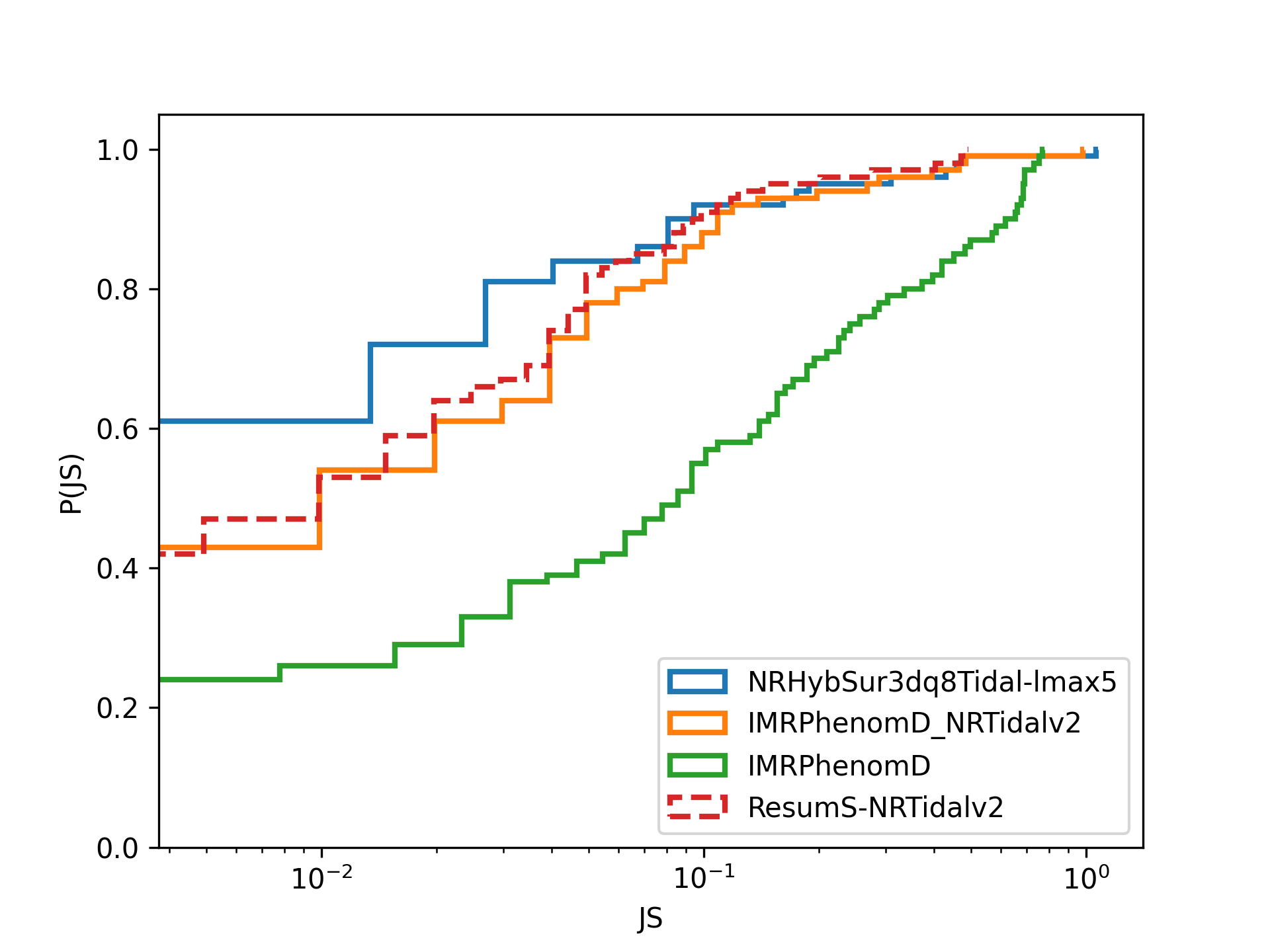
Figure 3 shows the cumulative distribution of combined JS divergences of parameters , q, and , between analyses performed with NRHybSur3dq8Tidal low amplitude injections. Specifically, the JS divergence is calculated between an analysis performed using precisely the same model used for injections on the one hand, and the alternative model listed in the legend on the other. Inferences performed with all state-of-the-art models that include tidal physics often produce qualitatively similar inferences, with JS divergences typically less than . Some relatively modest disagreement expected between (a) different waveform models and (b) the expected modest impact of higher-order modes for low-mass sources. By contrast, more than 10% of inferences have JS divergences larger than (mean over all parameters), in all cases when using models that include similar mode content (but a different waveform model). These calculations suggest that frequently, both waveform systematics and higher order modes produce noticably different results.
The green line in Figure 3 shows that tides must be included to avoid significantly biasing the interpretation of a typical low-amplitude source. This JS divergence corresponds to inferences that neglect tides entirely (via a point-particle IMRPhenomD model), even though the true full model includes tides. In this case, the JS divergence is frequently larger than , indicating substantial disagreement with the best possible interpretation.
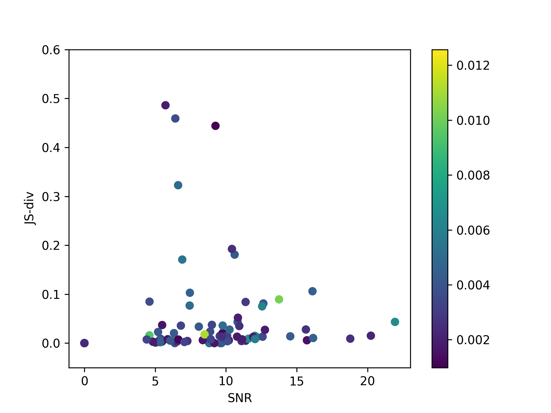
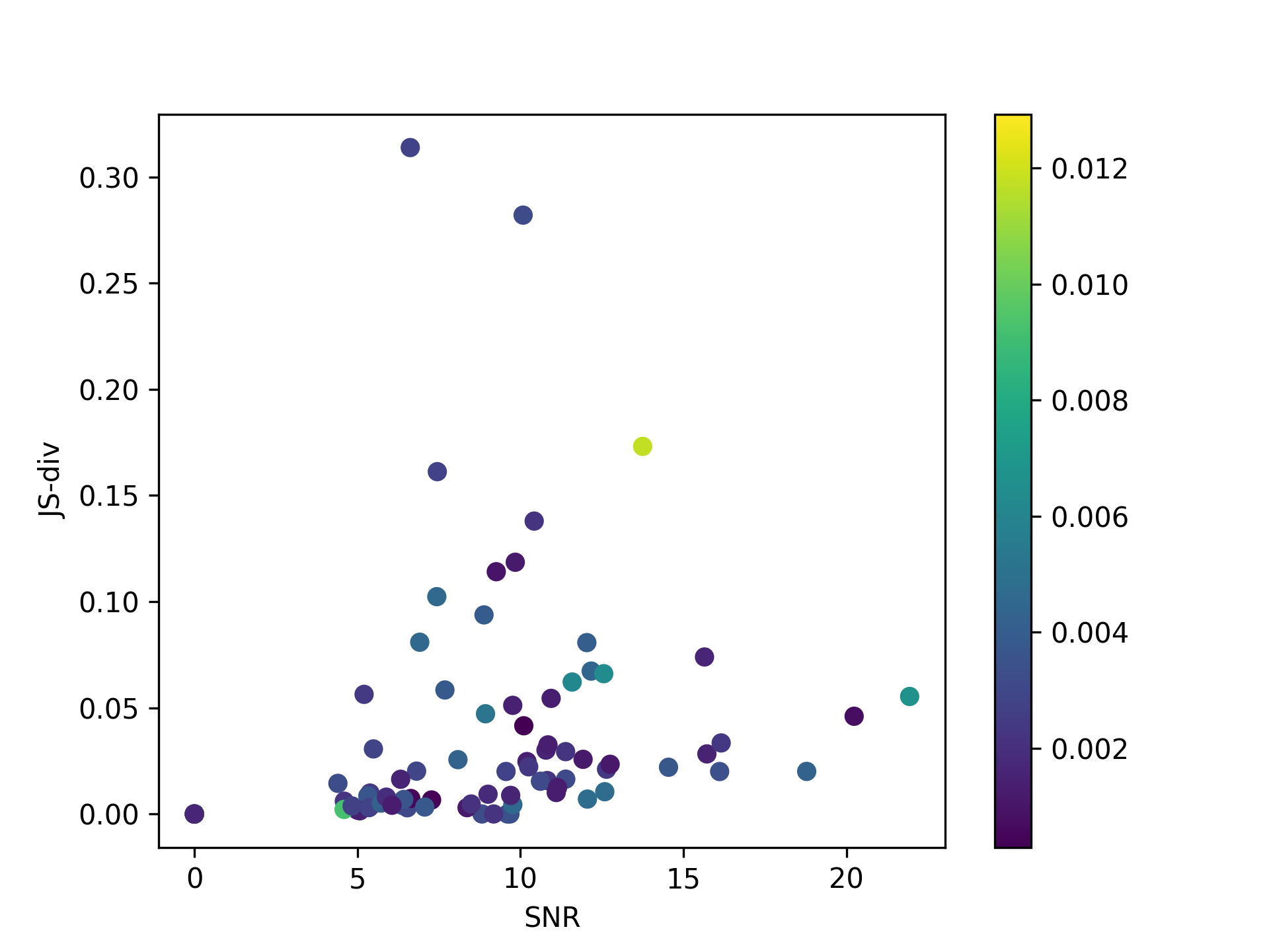
To investigate the impact of waveform systematics specifically, we computed mismatches between the injected and inference waveforms’ (2,2) modes. Mismatch is a simple inner-product-based estimate of waveform similarity between two model predictions Lindblom et al. (2008); Read et al. (2009); Lindblom et al. (2010); Cho et al. (2013); Hannam et al. (2010); Kumar et al. (2016); Pürrer and Haster (2020) and at identical model parameters :
| (3) |
In this expression, the inner product is implied by the kth detector’s noise power spectrum , which for the purposes of waveform similarity is assumed to be the advanced LIGO instrument, H1. In practice, we adopt a low-frequency cutoff so all inner products are modified to
| (4) |
The left panel of Figure 4 shows the results for NRHybSur3dq8Tidal injections recovered with TEOBResumS, with the mismatch shown as a color scale on top of the injected source SNR and cumulative JS divergence (summed over four one-dimensional JS divergences for parameters , q, and ). While the mismatches are within the waveform accuracy requirements Khan et al. (2016) for most of the injections(), higher mismatches don’t correlate well with extreme JS divergences. Rather, below some modest SNR, the random noise realization seems to interact adversely with these large mismatches to produce nearly unconstrained posteriors, such that the similarity between inferences becomes stochastic and diverges at low amplitude. The right panel of Figure 4 shows qualitatively similar behavior, using comparisons of NRHybSur3dq8Tidal and IMRPhenomD_NRTidalv2.
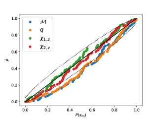
III.3 PP plots
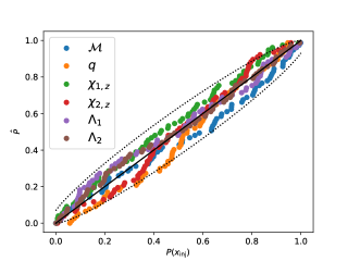
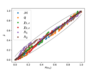
The differences between waveforms are significant enough that their imprint can even impact bulk diagnostics such as a PP plots Jan et al. (2020), which average the impact of waveform systematics over a large population of randomly chosen events.
Figures 5 and 6 provide another representation of the analyses presented above in the context of JS divergence: synthetic sources generated with the NRHybSur3dq8Tidal and TEOBResumS () models. In each panel, colored dots show the empirical cumulative distribution of the posterior quantiles of the injections – the PP plot for each parameter, with colors corresponding to the parameters indicated in the legend. Fig. 5 in which the same model was used for both injection and recovery for a particular panel, we see PP plots for every parameter are consistent with , as expected. However, Fig. 6 where analyses used IMRPhenomD for recovery, shows that omitting tidal physics entirely can bring in distinct inconsistencies with for injections where tides are significant and important.
IV Conclusions
In this paper, we demonstrated that the interpretation of typical low-amplitude BNS sources will frequently exhibit noteworthy differences, depending on the adopted model for analysis. Specifically, we showed that a JS divergence between inferences constructed between two different state-of-the-art waveforms would be larger than for a significant population of mergers. These large differences persist even though the mismatch between the dominant () mode of this state-of-the-art waveforms are small, and even though the SNR of our test sources is low. Additionally, corroborating previous work Dudi et al. (2018); Narikawa (2023), we demonstrate that tidal effects are essential to include even in interpreting our population of modest-SNR sources. Specifically, we showed that neglecting tidal physics in parameter inference causes a PP plot to deviate significantly from the expected diagonal behavior, indicating a biased recovery of mass and/or spin parameters.
Our study stands in contrast with the expectations of several previous studies, which have argued that the effects of waveform systematics for these low-mass, low-amplitude sources will be small. For example, investigations done in Gamba et al. (2021) suggest that systematic differences will supersede statistical differences for sources only for high SNR for the current GW detectors.
Our investigation only demonstrated notable differences in the conclusions derived from different waveform models. Further study is required to assess to what extent these differences propagate into conclusions derived from a population of sources or if they average out over the population.
Acknowledgements.
The authors would like to thank Carl-Johan Haster for helpful comments. ROS gratefully acknowledges support from NSF awards NSF PHY-1912632, PHY-2012057, and AST-1909534. AY acknowledges support from NSF PHY-2012057 grant. This material is based upon work supported by NSF’s LIGO Laboratory which is a major facility fully funded by the National Science Foundation. This research has made use of data, software and/or web tools obtained from the Gravitational Wave Open Science Center (https://www.gw-openscience.org/ ), a service of LIGO Laboratory, the LIGO Scientific Collaboration and the Virgo Collaboration. LIGO Laboratory and Advanced LIGO are funded by the United States National Science Foundation (NSF) as well as the Science and Technology Facilities Council (STFC) of the United Kingdom, the Max-Planck-Society (MPS), and the State of Niedersachsen/Germany for support of the construction of Advanced LIGO and construction and operation of the GEO600 detector. Additional support for Advanced LIGO was provided by the Australian Research Council. Virgo is funded through the European Gravitational Observatory (EGO), by the French Centre National de Recherche Scientifique (CNRS), the Italian Istituto Nazionale di Fisica Nucleare (INFN), and the Dutch Nikhef, with contributions by institutions from Belgium, Germany, Greece, Hungary, Ireland, Japan, Monaco, Poland, Portugal, Spain. The authors are grateful for computational resources provided by the LIGO Laboratory and supported by National Science Foundation Grants PHY-0757058, PHY-0823459 and PHY-1626190, and IUCAA LDG cluster Sarathi.References
- Abbott et al. (2016) (The LIGO Scientific Collaboration and the Virgo Collaboration) B. Abbott et al. (The LIGO Scientific Collaboration and the Virgo Collaboration), Phys. Rev. Lett 116, 061102 (2016).
- LIGO Scientific Collaboration et al. (2015) LIGO Scientific Collaboration, J. Aasi, B. P. Abbott, R. Abbott, T. Abbott, M. R. Abernathy, K. Ackley, C. Adams, T. Adams, P. Addesso, et al., Classical and Quantum Gravity 32, 074001 (2015), eprint 1411.4547.
- Accadia and et al (2012) T. Accadia and et al, Journal of Instrumentation 7, P03012 (2012), URL http://iopscience.iop.org/1748-0221/7/03/P03012.
- Acernese et al. (2015) F. Acernese et al. (VIRGO), Class. Quant. Grav. 32, 024001 (2015), eprint 1408.3978.
- The LIGO Scientific Collaboration et al. (2020a) The LIGO Scientific Collaboration, the Virgo Collaboration, B. P. Abbott, R. Abbott, T. D. Abbott, S. Abraham, F. Acernese, K. Ackley, C. Adams, V. B. Adya, et al., Phys. Rev. Lett 125, 101102 (2020a).
- The LIGO Scientific Collaboration et al. (2020b) The LIGO Scientific Collaboration, the Virgo Collaboration, B. P. Abbott, R. Abbott, T. D. Abbott, S. Abraham, F. Acernese, K. Ackley, C. Adams, V. B. Adya, et al., arXiv e-prints arXiv:2009.01190 (2020b), eprint 2009.01190.
- The LIGO Scientific Collaboration et al. (2020c) The LIGO Scientific Collaboration, the Virgo Collaboration, B. P. Abbott, R. Abbott, T. D. Abbott, S. Abraham, F. Acernese, K. Ackley, C. Adams, V. B. Adya, et al., Astrophysical Journal 896, L44 (2020c), URL https://doi.org/10.3847%2F2041-8213%2Fab960f.
- The LIGO Scientific Collaboration et al. (2020d) The LIGO Scientific Collaboration, the Virgo Collaboration, B. P. Abbott, R. Abbott, T. D. Abbott, S. Abraham, F. Acernese, K. Ackley, C. Adams, V. B. Adya, et al., Phys. Rev. D 102, 043015 (2020d).
- Abbott et al. (2021a) R. Abbott et al. (LIGO Scientific, VIRGO, KAGRA) (2021a), eprint 2111.03606.
- Shaik et al. (2019) F. H. Shaik, J. Lange, S. E. Field, R. O’Shaughnessy, V. Varma, L. E. Kidder, H. P. Pfeiffer, and D. Wysocki (2019), eprint 1911.02693.
- Williamson et al. (2017) A. Williamson, J. Lange, R. O’Shaughnessy, J. Clark, P. Kumar, J. Bustillo, and J. Veitch, Phys. Rev. D 96, 124041 (2017), URL https://journals.aps.org/prd/abstract/10.1103/PhysRevD.96.124041.
- Pürrer and Haster (2020) M. Pürrer and C.-J. Haster, Phys. Rev. Res. 2, 023151 (2020), eprint 1912.10055.
- Hannam et al. (2014) M. Hannam, P. Schmidt, A. Bohé, L. Haegel, S. Husa, F. Ohme, G. Pratten, and M. Pürrer, Phys. Rev. Lett 113, 151101 (2014), eprint 1308.3271.
- Khan et al. (2019) S. Khan, K. Chatziioannou, M. Hannam, and F. Ohme, Phys. Rev. D 100, 024059 (2019), eprint 1809.10113.
- Bohé et al. (2017) A. Bohé, L. Shao, A. Taracchini, A. Buonanno, S. Babak, I. W. Harry, I. Hinder, S. Ossokine, M. Pürrer, V. Raymond, et al., Phys. Rev. D 95, 044028 (2017), eprint 1611.03703.
- Varma et al. (2019) V. Varma, S. E. Field, M. A. Scheel, J. Blackman, D. Gerosa, L. C. Stein, L. E. Kidder, and H. P. Pfeiffer, Available as arxiv:1905.9300 (2019), eprint 1905.09300.
- Pratten et al. (2020) G. Pratten, C. García-Quirós, M. Colleoni, A. Ramos-Buades, H. Estellés, M. Mateu-Lucena, R. Jaume, M. Haney, D. Keitel, J. E. Thompson, et al., arXiv e-prints arXiv:2004.06503 (2020), eprint 2004.06503.
- Ossokine et al. (2020) S. Ossokine, A. Buonanno, S. Marsat, R. Cotesta, S. Babak, T. Dietrich, R. Haas, I. Hinder, H. P. Pfeiffer, M. Pürrer, et al., Phys. Rev. D 102, 044055 (2020), eprint 2004.09442.
- Wysocki et al. (2019a) D. Wysocki, J. Lange, and R. O’Shaughnessy, Phys. Rev. D 100, 043012 (2019a), URL https://arxiv.org/abs/1805.06442.
- Gamba et al. (2021) R. Gamba, M. Breschi, S. Bernuzzi, M. Agathos, and A. Nagar, Phys. Rev. D 103, 124015 (2021), eprint 2009.08467.
- Narikawa and Uchikata (2022) T. Narikawa and N. Uchikata, arXiv e-prints arXiv:2205.06023 (2022), eprint 2205.06023.
- Chatziioannou (2022) K. Chatziioannou, Phys. Rev. D 105, 084021 (2022), eprint 2108.12368.
- Kunert et al. (2022) N. Kunert, P. T. H. Pang, I. Tews, M. W. Coughlin, and T. Dietrich, Phys. Rev. D 105, L061301 (2022), eprint 2110.11835.
- Ashton and Dietrich (2021) G. Ashton and T. Dietrich, arXiv e-prints arXiv:2111.09214 (2021), eprint 2111.09214.
- Riemenschneider et al. (2021) G. Riemenschneider, P. Rettegno, M. Breschi, A. Albertini, R. Gamba, S. Bernuzzi, and A. Nagar, arXiv e-prints arXiv:2104.07533 (2021), eprint 2104.07533.
- Nagar et al. (2018) A. Nagar, S. Bernuzzi, W. Del Pozzo, G. Riemenschneider, S. Akcay, G. Carullo, P. Fleig, S. Babak, K. W. Tsang, M. Colleoni, et al., Phys. Rev. D 98, 104052 (2018), eprint 1806.01772.
- Barkett et al. (2020) K. Barkett, Y. Chen, M. A. Scheel, and V. Varma, Phys. Rev. D 102, 024031 (2020), eprint 1911.10440.
- Islam et al. (2021) T. Islam, S. E. Field, C.-J. Haster, and R. Smith, Phys. Rev. D 103, 104027 (2021), eprint 2010.04848.
- Lange et al. (2022) J. Lange, R. O’Shaughnessy, K. Barkett, V. Varma, and S. Field, in APS April Meeting Abstracts (2022), vol. 2022 of APS Meeting Abstracts, p. D17.007.
- Calderón Bustillo et al. (2021) J. Calderón Bustillo, S. H. W. Leong, T. Dietrich, and P. D. Lasky, Astrophys. J. Lett. 912, L10 (2021), eprint 2006.11525.
- Huang et al. (2021) Y. Huang, C.-J. Haster, S. Vitale, V. Varma, F. Foucart, and S. Biscoveanu, Phys. Rev. D 103, 083001 (2021), eprint 2005.11850.
- Samajdar and Dietrich (2018) A. Samajdar and T. Dietrich, Phys. Rev. D 98, 124030 (2018), eprint 1810.03936.
- Samajdar and Dietrich (2019) A. Samajdar and T. Dietrich, Phys. Rev. D 100, 024046 (2019), eprint 1905.03118.
- Dietrich et al. (2021) T. Dietrich, T. Hinderer, and A. Samajdar, Gen. Rel. Grav. 53, 27 (2021), eprint 2004.02527.
- Gamba et al. (2021) R. Gamba, M. Breschi, S. Bernuzzi, M. Agathos, and A. Nagar, Phys. Rev. D 103, 124015 (2021), eprint 2009.08467.
- Narikawa (2023) T. Narikawa (2023), eprint 2307.02033.
- Jan et al. (2020) A. Z. Jan, A. B. Yelikar, J. Lange, and R. O’Shaughnessy, Phys. Rev. D 102, 124069 (2020), eprint 2011.03571.
- Lange et al. (2018) J. Lange, R. O’Shaughnessy, and M. Rizzo, Submitted to PRD; available at arxiv:1805.10457 (2018).
- Wofford et al. (2023) J. Wofford, A. B. Yelikar, H. Gallagher, E. Champion, D. Wysocki, V. Delfavero, J. Lange, C. Rose, V. Valsan, S. Morisaki, et al., Phys. Rev. D 107, 024040 (2023).
- Wysocki et al. (2019b) D. Wysocki, R. O’Shaughnessy, J. Lange, and Y.-L. L. Fang, Phys. Rev. D 99, 084026 (2019b), eprint 1902.04934.
- Lange (2020) J. Lange, RIFT’ing the Wave: Developing and applying an algorithm to infer properties gravitational wave sources (2020), URL https://dcc.ligo.org/LIGO-P2000268.
- Dietrich et al. (2019) T. Dietrich, A. Samajdar, S. Khan, N. K. Johnson-McDaniel, R. Dudi, and W. Tichy, Phys. Rev. D 100, 044003 (2019), eprint 1905.06011.
- Dietrich et al. (2017) T. Dietrich, S. Bernuzzi, and W. Tichy, Phys. Rev. D 96, 121501 (2017), eprint 1706.02969.
- The LIGO Scientific Collaboration et al. (2017) The LIGO Scientific Collaboration, the Virgo Collaboration, B. P. Abbott, R. Abbott, T. D. Abbott, F. Acernese, K. Ackley, C. Adams, T. Adams, P. Addesso, et al., Phys. Rev. Lett 119, 161101 (2017).
- Abbott et al. (2020) B. P. Abbott, R. Abbott, T. D. Abbott, et al., ApJL 892, L3 (2020).
- Abbott et al. (2021b) R. Abbott et al. (LIGO Scientific, KAGRA, VIRGO), Astrophys. J. Lett. 915, L5 (2021b), eprint 2106.15163.
- LIGO Scientific Collaboration (2018) LIGO Scientific Collaboration (2018), URL https://dcc.ligo.org/LIGO-T1800044.
- Cook et al. (2006) S. Cook, A. Gelman, and D. Rubin, Journal of Computational and Graphical Statistics 15, 675 (2006), URL https://www.tandfonline.com/doi/abs/10.1198/106186006X136976.
- Ashton and Talbot (2021) G. Ashton and C. Talbot, Mon. Not. Roy. Astron. Soc. 507, 2037 (2021), eprint 2106.08730.
- The LIGO Scientific Collaboration et al. (2019) The LIGO Scientific Collaboration, The Virgo Collaboration, B. P. Abbott, R. Abbott, T. D. Abbott, F. Acernese, K. Ackley, C. Adams, T. Adams, P. Addesso, et al., Phys. Rev. X 9, 031040 (2019).
- Abbott et al. (2021) R. Abbott, T. D. Abbott, S. Abraham, F. Acernese, K. Ackley, A. Adams, C. Adams, R. X. Adhikari, et al. (LIGO Scientific, Virgo), Phys. Rev. X 11, 021053 (2021), eprint 2010.14527.
- Islam et al. (2023) T. Islam, A. Vajpeyi, F. H. Shaik, C.-J. Haster, V. Varma, S. E. Field, J. Lange, R. O’Shaughnessy, and R. Smith (2023), eprint 2309.14473.
- Lindblom et al. (2008) L. Lindblom, B. J. Owen, and D. A. Brown, Phys. Rev. D 78, 124020 (2008), eprint 0809.3844, URL http://xxx.lanl.gov/abs/arXiv:0809.3844.
- Read et al. (2009) J. S. Read, C. Markakis, M. Shibata, K. Uryū, J. D. E. Creighton, and J. L. Friedman, Phys. Rev. D 79, 124033 (2009), eprint 0901.3258.
- Lindblom et al. (2010) L. Lindblom, J. G. Baker, and B. J. Owen, Phys. Rev. D 82, 084020 (2010), eprint 1008.1803.
- Cho et al. (2013) H. Cho, E. Ochsner, R. O’Shaughnessy, C. Kim, and C. Lee, Phys. Rev. D 87, 02400 (2013), eprint 1209.4494, URL http://xxx.lanl.gov/abs/arXiv:1209.4494.
- Hannam et al. (2010) M. Hannam, S. Husa, F. Ohme, and P. Ajith, Phys. Rev. D 82, 124052 (2010), eprint 1008.2961.
- Kumar et al. (2016) P. Kumar, T. Chu, H. Fong, H. P. Pfeiffer, M. Boyle, D. A. Hemberger, L. E. Kidder, M. A. Scheel, and B. Szilagyi, Phys. Rev. D 93, 104050 (2016), eprint 1601.05396.
- Khan et al. (2016) S. Khan, S. Husa, M. Hannam, F. Ohme, M. Pürrer, X. J. Forteza, and A. Bohé, Phys. Rev. D 93, 044007 (2016), eprint 1508.07253.
- Dudi et al. (2018) R. Dudi, F. Pannarale, T. Dietrich, M. Hannam, S. Bernuzzi, F. Ohme, and B. Brügmann, Phys. Rev. D 98, 084061 (2018), eprint 1808.09749.