Andreev reflection, Andreev states, and long ballistic SNS junction

Abstract

The analysis in the present paper is based on the most known concept introduced by the brilliant physicist Alexander Andreev: Andreev bound states in a normal metal sandwiched between two superconductors. The paper presents results of direct calculations of ab initio expressions for the currents in a long ballistic SNS junction. The expressions are expanded in $1/L$ ($L$ is the thickness of the normal layer). The main contribution $\propto 1/L$ to the current agrees with the results obtained in the past, but the analysis suggests a new physical picture of the charge transport through the junction free from the problem with the charge conservation law. The saw-tooth current-phase relation at $T=0$ directly follows from the Galilean invariance of the Bogolyubov – de Gennes equations proved in the paper. The proof is valid for any variation of the energy gap in space if the Andreev reflection is the only scattering process. The respective roles of the contributions of bound and continuum states to the current are clarified. They depend on the junction dimensionality.

1 Introduction

The work of Andreev demonstrating the possibility of Andreev reflection was published nearly sixty years ago And64 . Remarkably, the interest to this phenomenon is not decreasing but rather increasing with time. More and more applications of it are being suggested. While in normal reflection a particle (quasiparticle) changes direction of its momentum, in the Andreev reflection it changes the direction of its group velocity. For reflection from an interface between a normal metal and a superconductor this means that a particle in a normal metal is reflected as a hole, or vice versa.

Andreev considered reflection from a planar interface. But it takes place also for quasiparticle reflection from a quantum vortex and not only in superconductors. Rotons in superfluid ⁴He have a spectrum similar to that of BCS quasiparticles. Andreev reflection from a velocity field around the vortex contributes to a force on the vortex from moving rotons in superfluid ⁴He and BCS quasiparticles in superconductors and in superfluid ³He. In fact, the first example of the Andreev reflection appeared in the paper by Lifshitz and Pitaevskii Lif57 on a force on a vortex from rotons even before Andreev’s paper And64 , although it is difficult to see this in their less-than-half page communication giving only final expressions for the force. Later calculations of this force with more details and some corrections were published Son75 ; Gal ; Kop76 ; EBS . Andreev reflection by vortices plays an important role in investigations of quantum turbulence in ³He, which is a Fermi superfluid described by the BCS theory Lancast . Recently Skrbek and Sergeev ScrbSerg suggested to use Andreev reflection of rotons by vortices in investigations of quantum turbulence in superfluid ⁴He.

The concept of Andreev reflection naturally brought Andreev to the next fundamental concept of condensed matter (and maybe not only condensed matter) physics: Andreev bound states And65 . In a normal metal between two superconductors quantum states with energies less than the gap in superconductors are not able to penetrate into the superconductor. Quasiparticles at these states jump forth and back with multiple Andreev reflections from interfaces. After any Andreev reflection a particle becomes a hole, or vice versa.

Andreev reflection and Andreev states are key concepts for the problem addressed in the present paper: long ballistic SNS junction (normal metal sandwiched between two superconductors). It was noticed long ago Kulik ; Ishii ; Bard that if the normal metal layer is ballistic the Josephson effect exists even for layer thickness much exceeding the coherence length. These works used the self-consistent field method deGen . In this method an effective pairing potential is introduced, which transforms the second-quantization Hamiltonian with the electron interaction into an effective Hamiltonian quadratic in creation and annihilation electron operators. The effective Hamiltonian can be diagonalized by the Bogolyubov – Valatin transformation.

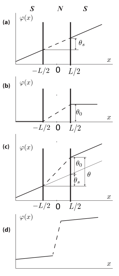
Figure 1: The phase variation across the SNS junction. (a) The condensate current produced by the phase gradient $\nabla\varphi$ in the superconducting layers. The phase $\theta_{s}=L\nabla\varphi$ is the superfluid phase. In all layers the electric current is equal to $env_{s}$. (b) The vacuum current produced by the phase $\theta_{0}=\theta_{+}-\theta_{-}$, which is called the vacuum phase. The current is confined to the normal layer, there is no current in superconducting layers. (c) The superposition of the condensate and the vacuum current. (d) The phase variation across a weak link.

The effective Hamiltonian is not gauge invariant, and the theory using this Hamiltonian violates the charge conservation law. The charge conservation law is restored if one solves the Bogolyubov – de Gennes equations together with the self-consistency equation for the pairing potential. In the past Kulik ; Ishii ; Bard this step was skipped. Instead of solving the self-consistency equation, it was postulated that there is a gap $\Delta$ of constant modulus $\Delta_{0}=\rvert\Delta\rvert$ in the superconducting layers and zero gap inside the normal layer. Further we use this idealized model assuming the following spatial variation of the gap in space (Fig. 1):

$$\Delta=\left\{\begin{array}[]{cc}\Delta_{0}e^{i\theta_{+}+i\nabla\varphi x}&x>L/2\\ 0&-L/2<x<L/2\\ \Delta_{0}e^{i\theta_{-}+i\nabla\varphi x}&x<-L/2\end{array}\right..$$ (1)

The effective masses and Fermi energies are equal in the superconductors and in the normal metal.

Previous theoretical investigations of the ballistic SNS junction have left some questions open:

1. Since the effective Hamiltonian is not gauge invariant, some solutions of the model violate the charge conservation law. They are mathematically correct, but are unphysical and must be filtered out. In many previous papers starting from the original ones Kulik ; Ishii ; Bard it was not done properly.

2. There was no clarity about the respective roles of bound and continuum states in the current in the normal layer. Ishii Ishii argued that both were important. This view was shared by a number of later publications (see Thuneberg Thun and references therein). But a clear quantitative analysis of the issue was still needed.

3. The effect of parity of Andreev levels (odd vs. even number of states) was not investigated or even mentioned. The effect is possible in the 1D case.

Reference Son21 addressed these issues recently. The analysis dealt directly with ab initio analytical expressions for relevant currents via sums and integrals over all bound and continuum states without introducing Green’s function formalism for their calculation as was mostly done in the past starting from Refs.  Kulik ; Ishii . Sums and integrals were calculated by expanding them in the inverse thickness $1/L$ of the normal layer.

In paper Son21 , a remedy for the violation of the conservation law in previous investigations was proposed. The strict conservation law was replaced by a softer condition that, at least, the total currents deep in all layers are the same. The condition can be satisfied only by taking into account three contributions to the total current $J=J_{s}+J_{v}+J_{q}$: (i) The current $J_{s}$ is induced by the phase gradient in the superconducting layers. It was called the Cooper-pair condensate, or simply the condensate current. (ii) The current $J_{v}$, which can flow in the normal layer even if the Cooper-pair condensate is at rest and all states are empty. It was called the vacuum current. (iii) The current $J_{q}$ induced by nonzero occupation of Andreev levels, i.e., by creation of quasiparticles. It was called the excitation current. Since the condensate motion produces the same current $J_{s}$ in all layers, while the vacuum and the excitation currents exist only in the normal layer, the charge conservation law requires that the sum of the vacuum and the excitation currents $J_{v}+J_{q}$ vanishes.

The solution of the Bogolyubov – de Gennes equations for the phase variation shown in Fig. 1(a) gives the state with the only condensate current $J_{s}=env_{s}$ in all layers. Here $n$ is the electron density and $v_{s}={\hbar\over 2m}\nabla\varphi$ is the superfluid velocity. This current does not differ from the current in a uniform superconductor since at Andreev scattering at interfaces between layers the Bogolyubov – de Gennes equations are Galilean invariant despite the translational invariance is broken Bard ; Son21 . The phase difference across the normal layer is $\theta_{s}=\nabla\varphi L$. It was called the superfluid phase Son21 . There is a state with the vacuum current $J_{v}$ flowing only in the normal layer [Fig. 1(b)], which is determined by the vacuum phase $\theta_{0}=\theta_{+}-\theta_{-}$ [see Eq. (1)]. The charge conservation law is violated if there is no excitation current compensating the vacuum current. Figure 1(c) shows the phase variation at the coexistence of the condensate and the vacuum current. The total phase difference across the normal layer is the Josephson phase $\theta=\theta_{s}+\theta_{0}$. The phase profiles in the normal layer are shown in Fig. 1 by dashed lines. This phase is not determined because it is a phase of the order parameter $\Delta$, which vanishes in the normal layer. Only the total phase difference across the normal layer appears in the Bogolyubov – de Gennes equations. The dashed lines simply show what the phase gradient would be if the normal metal were replaced by a superconductor.

In the past it was common to ignore the effect of the phase gradient in superconducting leads on the Josephson current. By default, it was supposed that this is not an issue because gradients in the leads are very small. This is true for a weak link, inside which the phase varies much faster than in the leads as shown in Fig. 1(d). At zero temperature the long SNS junction is not a weak link Son21 , and the phase gradient in the leads does affect the current in the normal layer. Thus, one should determine currents in the normal and superconducting layers self-consistently. The long ballistic SNS junction is a weak link only at high temperatures when the current is exponentially small.

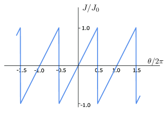
Figure 2: The saw-tooth current-phase relation at zero temperature. Here $J_{0}={\pi\hbar\over 2mL}en$ ($={ev_{f}\over L}$ in the 1D case).

Introduction of two phases $\theta_{0}$ and $\theta_{s}$ and the difference between the condensate and the vacuum current essentially revised the physical picture of charge transport through the ballistic SNS junction at zero temperature. The principal difference between two phases is that at tuning the phase $\theta_{0}$ Andreev levels move with respect to the gap, while at tuning the phase $\theta_{s}$ Andreev levels move together with the gap and their respective positions do not vary. All investigations predicted a saw-tooth current-phase relation (Fig. 2). But in the works Kulik ; Ishii ; Bard ignoring phase gradients in the leads, the current at sloped segments was a vacuum current calculated using the formalism of finite temperature Green’s functions. As argued above, the vacuum current cannot flow alone because this violates the charge conservation law. By contrast, according to Ref. Son21 , at sloped segments only the condensate current $J_{s}$ flows in all layers without violation of the charge conservation law. Its value directly follows from the Galilean transformation of the ground state in the condensate at rest to the state with moving condensate. As demonstrated in Sec. 3.1, the Bogolyubov – de Gennes equations are Galilean invariant if there is no normal scattering and the Andreev reflection is the only scattering process. The latter condition is satisfied if the ratio $\Delta_{0}/\varepsilon_{f}$ ($\varepsilon_{f}$ is the Fermi energy) is small. Thus, the derivation of the zero-temperature saw-tooth current-phase relation goes beyond the simple model of the step-function gap profile (Fig. 2) and is valid even if the gap profile is determined from the self-consistency equation. For derivation it is not necessary to first use the sophisticated theory for finite temperature Green functions in order to go to the limit $T\to 0$ in the end.

The vacuum current at zero temperature appears only at the vertical segments of the $T=0$ current-phase relation at $\theta=\pi(2s+1)$ ($s$ is an integer) when the energy of the lowest Andreev state reaches zero and its occupation becomes possible. This allows to satisfy the condition $J_{v}+J_{q}=0$.

The difference between the phases $\theta_{0}$ and $\theta_{s}$ was already considered in the past by Riedel et al. Bagwell although using a different terminology. They also realized an important difference between the point contact and the planar long ballistic SNS junction: the former is a weak link and the latter is not. This was illustrated by their Fig. 1, which is equivalent to our Figs. 1(a) and 1(d). The problem of charge conservation when the junction is not a weak link was discussed by Sols and Ferrer Sols for a superconductor interrupted by a barrier with high transmission probability.

Riedel et al. Bagwell went beyond the model with the postulated step-function dependence of the gap on the coordinate (Fig. 1) and numerically solved the Bogolyubov – de Gennes equations together with the integral self-consistency equation for the gap. Remarkably, they revealed that even though their numerics gave smoothly varying gap dependence in the transient interface between the normal layer and the superconducting leads, the phase gradient remained constant along the whole junction as in Fig. 1(a). This is a numerical confirmation of the Galilean invariance proved in Sec. 3.1 of the present paper analytically. Recently Davydova et al. diode also discussed the Galilean transformation (Doppler shift) for a short SNS junction shunted by a nanowire bridge. This setup was suggested for observation of the Josephson diode effect and essentially differs from that in the present paper. In their case the state with the only condensate current in all layers is absent.

Thuneberg published the Comment Thun rejecting the approach in Ref. Son21 and asserting that the vacuum current in continuum states was incorrectly ignored there (see the Reply Son23rep to the Comment). According to Son21 , in multidimensional (2D and 3D) cases the vacuum current in continuum states was suppressed after integrating over wave vectors transverse to the current through the junction. However, in the 1D case transverse degrees of freedom are absent, and the contribution of continuum states to the vacuum current does not vanish, but it was crudely estimated as insignificant in the limit $L\to\infty$. In the aftermath of the discussion with Thuneberg this estimation for the 1D case was re-accessed. It was revealed that the estimation missed an important term of the same order $\propto 1/L$ as the current in bound states. A more careful calculation of the vacuum current in continuum states is presented in this paper. Thus, Thuneberg Thun was vindicated in the 1D case. But the respective roles of bound and continuum states are different in the 1D and the multidimensional cases Son21 .

Discussing the controversy about respective contributions of bound and continuum states into the current, we have in mind only the vacuum current. As for the condensate current, it is clear that contributions of bound and continuum states into the current are proportional to their contributions to the density. The contribution of bound states to the density is less than the contribution of continuum states by the small factor $\Delta_{0}/\varepsilon_{f}$.

The re-evaluation of the contribution of continuum states to the vacuum current refuted the prediction Son21 that in the 1D case the ballistic long SNS junction becomes a $\varphi_{0}$ junction at high temperatures. The $\varphi_{0}$ junction is an anomalous Josephson junction, in which the ground state is not at zero phase. The prediction of a $\varphi_{0}$ junction was based on the existence of the large $\propto 1/L$ temperature-independent term in the excitation current with the sign opposite to the sign of the phase, which was not compensated by the vacuum current in bound states. However, according to the present analysis, the large negative excitation current is fully compensated by the positive continuum vacuum current, which was not taken into account in Ref. Son21 .

In Ref. Son21 the effect of incommensurability of the gap magnitude in the superconducting layers with respect to the Andreev level energy spacing was investigated in the 1D case. With tuning of the incommensurability parameter, the number of bound Andreev states varies being odd or even for every spin (the parity effect). This produces jumps on the current-phase relation. However, the present analysis reveals that the parity effect exists also in the continuum states, which were ignored in Ref. Son21 . Although there is no discrete states at energies exceeding the gap, there are peaks of the transmission probability for electrons crossing the normal layer (transmission resonances). The energy spacing between peaks is the same as the energy spacing between Andreev levels. While tuning phase, a new Andreev level appears (or an old one disappears) inside the gap, correspondingly some peak disappears (or a new one appears) in the continuum. As a result, the two parity effects compensate each other, and the total effect vanishes. Transmission peaks were known in the past Bard ; Svidz71 ; Kummel . Although the parity effect is cancelled in the total vacuum current, the effect yields important contributions $\propto 1/L$ to the currents in the bound and continuum states calculated separately.

The analysis in the paper is focused on the 1D case, where the only motion is along the axis $x$ normal to layers. For the extension of the calculation on multidimensional systems currents must be integrated over transverse components of wave vectors.

2 The Bogolyubov – de Gennes theory

In the self-consistent field method deGen the second-quantized effective Hamiltonian density quadratic in the wave function is

$${\cal H}_{eff}={\hbar^{2}\over 2m}[\nabla\hat{\psi}^{\dagger}_{\gamma}(x)\nabla\hat{\psi}_{\gamma}(x)-k_{f}^{2}\hat{\psi}^{\dagger}_{\gamma}(x)\hat{\psi}_{\gamma}(x)]$$

$$+\Delta\psi^{\dagger}_{\uparrow}(x)\psi^{\dagger}_{\downarrow}(x)+\Delta^{*}\psi_{\downarrow}(x)\psi_{\uparrow}(x),$$ (2)

where $\hat{\psi}_{\gamma}^{\dagger}(x)$ and $\hat{\psi}_{\gamma}(x)$ are operators of creation and annihilation of an electron, and the subscript $\gamma$ has two values corresponding to the spin up ($\uparrow$) and down ($\downarrow$). We address a 1D problem with the Fermi wave number $k_{f}$, assuming that our system is uniform in the plane normal to the axis $x$. In multidimensional systems with the Fermi wave number $k_{F}$ $k_{f}=\sqrt{k_{F}^{2}-k_{\perp}^{2}}$, where $k_{\perp}$ is the transverse component of the multidimensional wave vector $\bm{k}$.

The effective Hamiltonian can be diagonalized by the Bogolyubov – Valatin transformation from the free electron operators $\hat{\psi}_{\gamma}^{\dagger}(x)$ and $\hat{\psi}_{\gamma}(x)$ to the quasiparticle operators $\hat{a}_{i\gamma}^{\dagger}$ and $\hat{a}_{i\gamma}$:

$$\hat{\psi}_{\uparrow}(x)=\sum_{i}\left[u_{i}(x)\hat{a}_{i\uparrow}-v^{*}_{i}(x)\hat{a}^{\dagger}_{i\downarrow}\right],$$

$$\hat{\psi}_{\downarrow}(x)=\sum_{i}\left[u_{i}(x)\hat{a}_{i\downarrow}+v^{*}_{i}(x)\hat{a}^{\dagger}_{i\uparrow}\right].$$ (3)

The summation over the subscript $i$ means the summation over all bound and continuum states. The functions $u(x,t)$ and $v(x,t)$ are two components of a spinor wave function,

$$\psi(x,t)=\left[\begin{array}[]{c}u(x,t)\\ v(x,t)\end{array}\right],$$ (4)

describing a state of a quasiparticle, which is a superposition of a state with one particle (upper component $u$) and a state with one antiparticle, or hole (lower component $v$). They are stationary solutions of the Bogolyubov – de Gennes equations:

$$i\hbar{\partial u\over\partial t}={\delta{\cal H}_{BG}\over\delta u^{*}}=-{\hbar^{2}\over 2m}\left(\nabla^{2}+k_{f}^{2}\right)u+\Delta v,$$

$$i\hbar{\partial v\over\partial t}={\delta{\cal H}_{BG}\over\delta v^{*}}={\hbar^{2}\over 2m}\left(\nabla^{2}+k_{f}^{2}\right)v+\Delta^{*}u.$$ (5)

The Bogolyubov – de Gennes equations are the Hamilton equations with the Hamiltonian (per unit volume)

$${\cal H}_{BG}={\hbar^{2}\over 2m}(\lvert\nabla u\rvert^{2}-k_{f}^{2}\lvert u\rvert^{2})-{\hbar^{2}\over 2m}(\lvert\nabla v\rvert^{2}-k_{f}^{2}\lvert v\rvert^{2})+\Delta u^{*}v+\Delta^{*}v^{*}u.$$ (6)

The number of particles (charge) is not a quantum number of the state. The average density $n_{i}$ and current $j_{i}$ in the $i$th state are

$$n_{i}=\lvert u_{i}\rvert^{2}-\lvert v_{i}\rvert^{2},$$ (7)

and

$$j_{i}=-{ie\hbar\over 2m}(u_{i}^{*}\nabla u_{i}-u_{i}\nabla u_{i}^{*})-{ie\hbar\over 2m}(v_{i}^{*}\nabla v_{i}-v_{i}\nabla v_{i}^{*}).$$ (8)

After the diagonalization the effective Hamiltonian becomes

$${\cal H}_{eff}=\sum_{i}\varepsilon_{i}(a^{\dagger}_{i\uparrow}a_{i\uparrow}+a^{\dagger}_{i\downarrow}a_{i\downarrow}-2\lvert v\rvert^{2}),$$ (9)

where $\varepsilon_{i}$ is the energy of the $i$th quasiparticle state.

The total density $n$ and the total charge current $J$ are expectation values for the operators

$$\hat{n}(x)=\hat{\psi}^{\dagger}_{\uparrow}(x)\hat{\psi}_{\uparrow}(x)+\hat{\psi}^{\dagger}_{\downarrow}(x)\hat{\psi}_{\downarrow}(x)$$

$$=\sum_{i}\left[\lvert u_{i}(x)\rvert^{2}(\hat{a}^{\dagger}_{i\uparrow}\hat{a}_{i\uparrow}+\hat{a}^{\dagger}_{i\downarrow}\hat{a}_{i\downarrow})+\lvert v_{i}(x)\rvert^{2}(\hat{a}_{i\uparrow}\hat{a}^{\dagger}_{i\uparrow}+\hat{a}_{i\downarrow}\hat{a}^{\dagger}_{i\downarrow})\right]$$

$$=\sum_{i}\left\{[\lvert u_{i}(x)\rvert^{2}-\lvert v_{i}(x)\rvert^{2}](\hat{a}^{\dagger}_{i\uparrow}\hat{a}_{i\uparrow}+\hat{a}^{\dagger}_{i\downarrow}\hat{a}_{i\downarrow})+2\lvert v_{i}(x)\rvert^{2}\right\},$$ (10)

$$\hat{J}=-{ie\hbar\over 2m}\sum_{i}\left[(u_{i}^{*}\nabla u_{i}-u_{i}\nabla u_{i}^{*}+v_{i}^{*}\nabla v_{i}-v_{i}\nabla v_{i}^{*})(\hat{a}^{\dagger}_{i\uparrow}\hat{a}_{i\uparrow}+\hat{a}^{\dagger}_{i\downarrow}\hat{a}_{i\downarrow})\right.$$

$$\left.-2(v_{i}^{*}\nabla v_{i}-v_{i}\nabla v_{i}^{*})\right].$$ (11)

There are two contributions to the energy, the density, and the current [Eqs. (9)–(11)]. One is connected with the quasiparticle vacuum, in which all energy levels are not occupied (last terms in equations without operators). This contribution is responsible for the condensate and the vacuum current. The other terms in the equations are connected with quasiparticles occupying energy levels. They are responsible for the excitation current.

In a uniform superconductor at rest, the constant $\Delta_{0}$ solutions of the Bogolyubov – de Gennes equations are plane waves

$$\left(\begin{array}[]{c}u_{0}\\ v_{0}\end{array}\right)e^{ik\cdot x-i\varepsilon_{0}t/\hbar},$$ (12)

where

$$u_{0}=\sqrt{{1\over 2}\left(1+{\xi\over\varepsilon_{0}}\right)},~{}~{}v_{0}=\sqrt{{1\over 2}\left(1-{\xi\over\varepsilon_{0}}\right)}.$$ (13)

The quasiparticle energy is given by the well known BCS expression:

$$\varepsilon_{0}=\sqrt{\xi^{2}+\Delta_{0}^{2}}.$$ (14)

Here $\xi=({\hbar^{2}/2m})(k^{2}-k_{f}^{2})\approx\hbar v_{f}(k-k_{f})$ is the quasiparticle energy in the normal Fermi liquid, and $v_{f}=\hbar k_{f}/m$ is the Fermi velocity. The states with positive and the negative signs of $\xi$ correspond to particle-like and the hole-like branches of the spectrum respectively.

The Bogolyubov – de Gennes equations have also solutions with negative energies $\varepsilon_{0}=-\sqrt{\xi^{2}+\Delta_{0}^{2}}$. In a stable state, energies of all excitations must be positive, and solutions with negative energies should not be considered Tin .

3 Ab initio expressions for currents

3.1 Galilean invariance and condensate current

An important assumption in the present analysis (as well as in the previous investigations) was that only the Andreev reflection is possible on interfaces between superconducting and normal layers. The assumption is valid in the limit of large Fermi wave numbers $k_{f}\gg\Delta_{0}/\hbar v_{f}$. As mentioned in Introduction, this means that there is no significant change of the quasiparticle momentum after reflection, and wave functions $\left(\begin{array}[]{c}u\\ v\end{array}\right)$ are superpositions of plane waves with wave numbers only close to either $+k_{f}$, or $-k_{f}$. These plane waves describe quasiparticles, which will be called rightmovers (+) and leftmovers (-). After transformation of the wave function,

$$\left(\begin{array}[]{c}u\\ v\end{array}\right)=\left(\begin{array}[]{c}\tilde{u}\\ \tilde{v}\end{array}\right)e^{\pm ik_{f}x},$$ (15)

the second order terms in gradients, $\nabla^{2}\tilde{u}$ and $\nabla^{2}\tilde{v}$, can be neglected for small $\Delta_{0}/\varepsilon_{f}$, and the Bogolyubov – de Gennes equations are reduced to the equations of the first order in gradients:

$$\varepsilon\tilde{u}=\mp i\hbar v_{f}\nabla\tilde{u}+\Delta\tilde{v},$$

$$\varepsilon\tilde{v}=\pm i\hbar v_{f}\nabla\tilde{v}+\Delta^{*}\tilde{u}.$$ (16)

The boundary conditions on the interfaces between layers require the continuity of the wave function components, but not their gradients.

Let us demonstrate Galilean invariance of the Bogolyubov – de Gennes equations when the wave functions are superpositions of only rightmovers, or only of leftmovers. Suppose that we found the Bogolyubov – de Gennes function $\left(\begin{array}[]{c}\tilde{u}_{0}\\ \tilde{v}_{0}\end{array}\right)$ with the energy $\varepsilon_{0}$ for an arbitrary profile of the superconducting gap $\Delta(x)$. Now we check what is the solution of the Bogolyubov – de Gennes equations for the superconducting gap $\Delta(x)e^{i\nabla\varphi x}$, where $\nabla\varphi$ is a constant phase gradient. The wave function

$$\left(\begin{array}[]{c}\tilde{u}\\ \tilde{v}\end{array}\right)=\left(\begin{array}[]{c}\tilde{u}_{0}e^{i\nabla\varphi x/2}\\ \tilde{v}_{0}e^{-i\nabla\varphi x/2}\end{array}\right)$$ (17)

satisfies Eq. (16) where the gap $\Delta(x)$ is replaced by $\Delta(x)e^{i\nabla\varphi x}$ and the energy is

$$\varepsilon=\varepsilon_{0}\pm{\hbar v_{f}\over 2}\nabla\varphi=\varepsilon_{0}\pm{\hbar v_{f}\over 2L}\theta_{s}=\varepsilon_{0}\pm v_{s}\hbar k_{f}.$$ (18)

Thus, the Galilean transformation produces the same Doppler shift in the energy as in a uniform superconductor. According to Eqs. (7) and (8) for the density $n_{i}$ and the current $j_{i}$ in the $i$th Bogolyubov – de Gennes state, the Galilean transformation transforms the current $j_{i}$ to the current $j_{i}+en_{i}v_{s}$. Summation over all bound and continuum states yields that the Galilean transformation added the condensate current $J_{s}=env_{s}$ in the whole space. The difference between the total charge densities $n$ in the normal and the superconducting layers vanishes in the limit $L\to\infty$ Son21 . Thus, the condensate current is the same in all layers and does not violate the charge conservation law.

Our derivation does not depend on the profile of the gap in the space, as far as the gap is small compared to the Fermi energy and there is no normal scattering transforming rightmovers into leftmovers and vice versa. The Doppler shift of the energy is of opposite sign for rightmovers and leftmovers, and after the Galilean transformation of a superposition of rightmovers and leftmovers the state is not an eigenstate of the energy. The derivation remains valid if $\Delta$ vanishes in some part of the space. Independence of the condensate current on the gap profile is confirmed by numerical solution of the Bogolyubov – de Gennes equations together with the integral self-consistency equation for the gap by Riedel et al Bagwell , as already mentioned in Sec. 1. They obtained that although the absolute value of the gap smoothly varies between the normal layer and the superconducting leads, the phase gradient is constant in all layers as in Fig. 1(a). Summarizing, the value of the condensate current directly follows from the Galilean invariance and does not need sophisticated calculations.

3.2 Vacuum current in bound states

The spectrum and the wave functions for the present model of the SNS junction are well known from previous works, and it is sufficient here to present the resume of these investigations. Solving the Bogolyubov – de Gennes equations with the gap profile given by Eq. (1) for zero gradient $\nabla\varphi$ (Cooper-pair condensate at rest) and with the boundary conditions formulated above one finds the equation for energies $\varepsilon_{0\pm}(s)$ of bound Andreev states:

$$\varepsilon_{0\pm}(s)={\hbar v_{f}\over 2L}\left[2\pi s+\arcsin{\sqrt{\Delta_{0}^{2}-\varepsilon_{0\pm}(s)^{2}}\over\Delta_{0}}\pm\theta_{0}\right].$$ (19)

Here $s$ is an integer. The upper and the lower signs correspond to rightmovers (+) and leftmovers (-) respectively. If the condensate moves ($\nabla\varphi\neq 0$) the energy $\varepsilon_{\pm}(s)$ of the state is given by Eq. (18):

$$\varepsilon_{\pm}(s)={\hbar v_{f}\over 2L}\left[2\pi s+\arcsin{\sqrt{\Delta_{0}^{2}-\varepsilon_{0\pm}(s)^{2}}\over\Delta_{0}}\pm\theta\right].$$ (20)

The phase in the equation for $\varepsilon_{0\pm}(s)$ is $\theta_{0}$, while the energy $\varepsilon_{\pm}(s)$ depends on the total Josephson phase $\theta=\theta_{0}+\nabla\varphi L=\theta_{0}+\theta_{s}$.

At small energy $\varepsilon_{0\pm}(s)\ll\Delta_{0}$ (small $s$)

$$\varepsilon_{0\pm}(s)={\hbar v_{f}\over 2L}\left[2\pi\left(s+{1\over 2}\right)\pm\theta_{0}\right].$$ (21)

For Andreev levels close to the gap one can expand the arcsin function in Eq. (19) transforming it to

$$\Delta_{0}-\varepsilon_{0\pm}-{\zeta_{0}\over L}\sqrt{2\Delta_{0}(\Delta_{0}-\varepsilon_{0\pm})}=\Delta_{0}-\pi s{\zeta_{0}\over L}\Delta_{0}=\pi(t+\alpha){\zeta_{0}\over L}\Delta_{0}.$$ (22)

Here $\alpha$ ($0<\alpha<1$) is the parameter of incommensurability, which is the fractional part of the ratio of the gap $\Delta_{0}$ to the Andreev level energy spacing,

$${\Delta_{0}L\over\pi\hbar v_{f}}={L\over\pi\zeta_{0}}=s_{m}+\alpha,$$ (23)

$s_{m}$ is the maximal integer less than the ratio, $t=s_{m}-s$ is another integer, and

$$\zeta_{0}={\hbar v_{f}\over\Delta_{0}}$$ (24)

is the coherence length. Solution of Eq. (22) yields

$$\varepsilon_{0\pm}=\Delta_{0}-{\pi\zeta_{0}\over L}\Delta_{0}\left[\sqrt{t+\alpha\mp{\theta_{0}\over 2\pi}+{\zeta_{0}\over 2\pi L}}-\sqrt{{\zeta_{0}\over 2\pi L}}\right]^{2},$$

$$\sqrt{\Delta_{0}^{2}-\varepsilon_{0\pm}^{2}}=\Delta_{0}\sqrt{2\pi\zeta_{0}\over L}\left[\sqrt{t+\alpha\mp{\theta_{0}\over 2\pi}+{\zeta_{0}\over 2\pi L}}-\sqrt{\zeta_{0}\over 2\pi L}\right].$$ (25)

There is an essential difference between effects of phases $\theta_{0}$ and $\theta_{s}$ on the Andreev spectrum Son21 . Variation of $\theta_{0}$ makes the Andreev levels to move with respect to the gap. As a result, some new levels can emerge and some old ones can disappear. In contrast, variation of $\theta_{s}$ leads to the shift of the spectrum as a whole without changing positions of Andreev levels with respect to the gap. The principle of the BCS theory that only solutions with positive energies should be taking into account refers to the energy $\varepsilon_{0}$, while the Doppler-shifted energy $\varepsilon$ can be both positive or negative. If $\varepsilon$ is negative the level is occupied at zero temperature.

The current in the Andreev state is determined by the canonical relation connecting it with the derivative of the energy with respect to the phase:

$$j_{\pm}(s)={2e\over\hbar}{\partial\varepsilon_{0\pm}(s)\over\partial\theta_{0}}=\pm{e\over\pi\hbar}{\partial\varepsilon_{0\pm}(s)\over\partial s}=\pm{ev_{f}\over L+\zeta}=\pm{ev_{f}\over L}\frac{\sqrt{1-{\varepsilon_{0\pm}(s)^{2}\over\Delta_{0}^{2}}}}{\sqrt{1-{\varepsilon_{0\pm}(s)^{2}\over\Delta_{0}^{2}}}+{\zeta_{0}\over L}}.$$ (26)

Here

$$\zeta=\zeta_{0}{\Delta_{0}\over\sqrt{\Delta_{0}^{2}-\varepsilon_{0}^{2}}}$$ (27)

is the depth of penetration of the bound states into the superconducting layers, which diverges when $\varepsilon_{0}$ approaches to the gap $\Delta_{0}$. The factor 2 takes into account that $\theta_{0}$ is the phase of a Cooper pair but not of a single electron.

The current $j_{\pm}(s)$ is a current produced by a quasiparticle created at the $s$th state. However, we look for the vacuum current when there is no quasiparticles. In Andreev states $|u\rvert^{2}=|v\rvert^{2}={1\over 2}$, and according to Eq. (11) the vacuum current in any state is two times less, and it has a sign opposite to the sign of the current $j_{\pm}(s)$. Taking this into account and including two spin states, the ab initio expression for the vacuum current in bound states is

$$J_{vA}=-\sum_{s}\{j_{+}(s)\mbox{H}[\varepsilon_{0+}(s)]\mbox{H}[\Delta_{0}-\varepsilon_{0+}(s)]+j_{-}(s)\mbox{H}[\varepsilon_{0-}(s)]\mbox{H}[\Delta_{0}-\varepsilon_{0-}(s)]\}$$

$$=-{ev_{f}\over L}\sum_{s}\left\{\frac{\sqrt{1-{\varepsilon_{0+}(s)^{2}\over\Delta_{0}^{2}}}}{\sqrt{1-{\varepsilon_{0+}(s)^{2}\over\Delta_{0}^{2}}}+{\zeta_{0}\over L}}\mbox{H}[\varepsilon_{0+}(s)]\mbox{H}[\Delta_{0}-\varepsilon_{0+}(s)]\right.$$

$$\left.-\frac{\sqrt{1-{\varepsilon_{0-}(s)^{2}\over\Delta_{0}^{2}}}}{\sqrt{1-{\varepsilon_{0-}(s)^{2}\over\Delta_{0}^{2}}}+{\zeta_{0}\over L}}\mbox{H}[\varepsilon_{0-}(s)]\mbox{H}[\Delta_{0}-\varepsilon_{0-}(s)]\right\}.~{}~{}~{}$$ (28)

Here $\mbox{H}(q)$ is the Heaviside step function, which ensures that summation over $s$ extends only on states with energies $0<\varepsilon_{0\pm}<\Delta_{0}$ inside the gap.

3.3 Continuum vacuum current

According to Refs. Bard ; Son21 ; Bagw , for a rightmover quasiparticle ($\xi>0$) incident from left the transmission and the reflection probabilities are

$${\cal T}(\theta_{0})=\frac{2(\varepsilon_{0}^{2}-\Delta_{0}^{2})}{2\varepsilon_{0}^{2}-\Delta_{0}^{2}-\Delta_{0}^{2}\cos\left({2\varepsilon_{0}mL\over\hbar^{2}k_{f}}-\theta_{0}\right)},~{}~{}R(\theta_{0})=1-{\cal T}(\theta_{0}).$$ (29)

These expressions are valid also for a quasihole ($\xi<0$) incident from right. For a quasiparticle incident from right and a hole incident from left the transmission and the reflection probabilities are ${\cal T}(-\theta_{0})$ and $R(-\theta_{0})$.

Equation (29) was obtained in the coordinate frame moving with the condensate. Transformation to the laboratory frame leads to replacing of the argument ${2\varepsilon_{0}mL\over\hbar^{2}k_{f}}-\theta_{0}$ of the cosine function by ${2\varepsilon mL\over\hbar^{2}k_{f}}-\theta$. According to Eq. (18) they are equal. Thus, the Galilean transformation discussed in Sec. 3.1 does not change the scattering parameters.

One can transform expressions for ${\cal T}$ and $R$ revealing their dependence on the incommensurability parameter $\alpha$ introduced in Eq. (23):

$${\cal T}(\theta_{0})=\frac{2(\varepsilon_{0}^{2}-\Delta_{0}^{2})}{2\varepsilon_{0}^{2}-\Delta_{0}^{2}-\Delta_{0}^{2}\cos\left[{2(\varepsilon_{0}-\Delta_{0})mL\over\hbar^{2}k_{f}}+2\pi\alpha-\theta_{0}\right]}.$$ (30)

The reflection probability can be transformed similarly. The both probabilities rapidly oscillate as functions of the energy.

Collecting together all contributions from rightmovers and leftmovers, quasiparticles and quasiholes, the ab initio expression for the continuum vacuum current is Son21

$$J_{vC}={e\over\pi\hbar}\int_{\Delta_{0}}^{\infty}[{\cal T}(-\theta_{0})-{\cal T}(\theta_{0})]d\xi.$$ (31)

3.4 Excitation current

As well as in previous literature, the present analysis addresses the case when temperatures are much lower than critical ($T\ll\Delta_{0}$). Then one can ignore excitations in continuum states and replace sums for a large but finite number of Andreev states by infinite sums. The ab initio expression for the excitation current assumes the Fermi distribution in Andreev levels:

$$J_{q}=\sum_{s=0}^{\infty}\frac{j_{+}(s)}{e^{\varepsilon_{+}(s)/T}+1}+\sum_{s=0}^{\infty}\frac{j_{-}(s)}{e^{\varepsilon_{-}(s)/T}+1}.$$ (32)

The currents $j_{\pm}(s)$ in the $s$th state are given by Eq. (26) derived for the condensate at rest despite this expression is for the case of a moving condensate. This is because in Andreev states $\lvert u\rvert^{2}=\lvert v\rvert^{2}$, and according to Eq. (7) quasiparticle creation in an Andreev state does not change the electron density. Thus, the Galilean transformation does not change the electron current of the quasiparticle. At $T\ll\Delta_{0}$ the expression Eq. (21) for the small energy $\varepsilon_{0\pm}$ can be used, and taking into account the relation Eq. (18) between $\varepsilon_{\pm}(s)$ and $\varepsilon_{0\pm}(s)$, the excitation current is

$$J_{q}={2ev_{f}\over L}\sum\limits_{0}^{\infty}\left[\frac{1}{e^{\beta\left(s+{\pi+\theta\over 2\pi}\right)}+1}-\frac{1}{e^{\beta\left(s+{\pi-\theta\over 2\pi}\right)}+1}\right],$$ (33)

where

$$\beta={\pi\hbar v_{f}\over LT}.$$ (34)

While the vacuum current depends from the vacuum phase $\theta_{0}$, the excitation current depends on the total Josephson phase $\theta=\theta_{0}+\theta_{s}$.

4 Calculation of vacuum and excitation currents

Through the whole paper we assume in calculations that $0<\alpha<1/2$ and $\theta_{0}<\pi$. If $1/2<\alpha<1$ currents of rightmovers and leftmovers will be different, but their sum will be the same as for $0<1-\alpha<1/2$. As for the dependence on $\theta_{0}$, its extension on the infinite interval of $\theta_{0}$ is straightforward bearing in mind that the current is an odd periodic function of $\theta_{0}$.

4.1 Vacuum current in bound Andreev states

Calculating the vacuum current in bound Andreev states one can expand the current in $1/L$. In Ref. Son21 the first terms $J_{1}\propto 1/L$ and $J_{3/2}\propto 1/L^{3/2}$ were calculated:

$$J_{vA}=J_{1}+J_{3/2}.$$ (35)

where

$$J_{1}={ev_{f}\over L}\mbox{H}(-\gamma_{+}),$$ (36)

and

$$J_{3/2}={e\Delta_{0}\zeta_{0}^{3/2}\over\sqrt{2\pi}\hbar L^{3/2}}\left[\sum_{t=0}^{\infty}\left(\frac{1}{\sqrt{t+{\gamma_{+}\over 2\pi}}}-\frac{1}{\sqrt{t+{\gamma_{-}\over 2\pi}}}\right)-\sqrt{2\pi\over\gamma_{+}}\mbox{H}\left(-\gamma_{+}\right)\right]$$

$$={e\Delta_{0}\zeta_{0}^{3/2}\over\sqrt{2\pi}\hbar L^{3/2}}\left[\zeta\left({1\over 2},{\gamma_{+}\over 2\pi}\right)-\zeta\left({1\over 2},{\gamma_{-}\over 2\pi}\right)-\sqrt{2\pi\over\gamma_{+}}\mbox{H}\left(-\gamma_{+}\right)\right].$$ (37)

Here

$$\gamma_{\pm}=2\pi\alpha\mp\theta_{0},$$ (38)

and

$$\zeta\left(z,q\right)=\sum_{t=0}^{\infty}{1\over(q+t)^{z}}$$ (39)

is Riemann’s zeta function 5 . The series for Riemann’s zeta function at $z=1/2$ diverges, but the series for a difference of zeta functions with different arguments $q$ converges at large $t$. It was taken into account that the main contribution to the sum in Eq. (37) is given by Andreev levels close the gap, where one can use the expression Eq. (25) for $\varepsilon_{0\pm}(s)$.

At small positive $\gamma_{+}=2\pi\alpha-\theta_{0}\ll 1$ (but still $\gamma_{+}\gg\zeta_{0}/L$) the current $J_{3/2}$ is determined only by the term $t=0$ divergent in the limit $\gamma_{+}\to 0$:

$$J_{3/2}={e\Delta_{0}\zeta_{0}^{3/2}\over\hbar L^{3/2}\sqrt{\gamma_{+}}}.$$ (40)

Later we shall see that the current $J_{3/2}$ in the bound states is compensated by the $\propto 1/L^{3/2}$ current in continuum states.

4.2 Continuum vacuum current

The continuum vacuum current is a difference of contributions from right- and leftmovers:

$$J_{vC}=J_{+}-J_{-},~{}~{}J_{\pm}=-{e\over\pi\hbar}\int_{\Delta_{0}}^{\infty}{\cal T}(\pm\theta_{0})d\xi.$$ (41)

Calculating $J_{\pm}$ we introduce a new variable $z=(\varepsilon_{0}-\Delta_{0})/\Delta_{0}$:

$$J_{\pm}=-{e\Delta_{0}\over\pi\hbar}\int_{0}^{x_{m}}\frac{2\sqrt{2z+z^{2}}(1+z)\,dz}{4z+2z^{2}+1-\cos(2Lz/\zeta_{0}+\gamma_{\pm})}.$$ (42)

The integrals for $J_{\pm}$ diverge, but their difference does not. So, we introduced a large $x_{m}$ as an upper limit of integrals assuming that in the end $x_{m}\to\infty$.

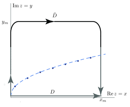
Figure 3: Analytical continuation in the complex plane $z=x+iy$ of the path for the integration in Eq. (42). Black circles on the dashed line are poles.

For calculation of the integrals we perform an analytical continuation from the real axis (contour $D$ in Fig. 3) to the complex plane $z=x+iy$ (contour $\bar{D}$ in Fig. 3). Calculating contributions of various segments of the contour we need to take into account only their real parts. The final integral Eq. (42) is real, and the total sum of imaginary parts must vanish.

At the continuation the contour crosses poles in points $z_{p\pm}=x_{p\pm}+iy_{p\pm}$. The values of $z_{p\pm}$ are roots of the equation

$$1+4z_{p\pm}+2z_{p\pm}^{2}-\cos\left(2Lz_{p\pm}/\zeta_{0}+\gamma_{\pm}\right)=0,$$ (43)

where $p$ is an integer number of a pole. At $L\to\infty$ the coordinates of poles are

$$x_{p\pm}={\zeta_{0}\over 2L}(2\pi p-\gamma_{\pm}),~{}~{}y_{p\pm}={\zeta_{0}\over L}\ln(\sqrt{2x_{p\pm}+x_{p\pm}^{2}}+1+x_{p\pm}).$$ (44)

Residues of poles are

$${\cal R}_{p\pm}=-{e\Delta_{0}\over\pi\hbar}\frac{2\sqrt{z_{p\pm}(2+z_{p\pm})}(1+z_{p\pm})}{4+4z_{p\pm}+{2L\over\zeta_{0}}\sin\left(2Lz_{p\pm}/\zeta_{0}+\gamma_{\pm}\right)}$$

$$=-{e\Delta_{0}\over\pi\hbar}\frac{2\sqrt{z_{p\pm}(2+z_{p\pm})}(1+z_{p\pm})}{4+4z_{p\pm}+{2iL\over\zeta_{0}}\sqrt{(1+4z_{p\pm}+2z_{p\pm}^{2})^{2}-1}}$$

$$=-{e\Delta_{0}\over 2\pi\hbar}\frac{\zeta_{0}\sqrt{z_{p\pm}(2+z_{p\pm})}}{iL\sqrt{z_{p\pm}(2+z_{p\pm})}+\zeta_{0}}\approx{iev_{f}\over 2\pi L}.$$ (45)

The contribution of poles to the current,

$$J_{R\pm}=-2\pi\mbox{Im}\sum_{p}{\cal R}_{p\pm}=-{ev_{f}\over L}p_{\pm},$$ (46)

is determined by the numbers $p_{\pm}$ of poles for rightmovers and leftmovers. Corrections to the total current $J_{R+}-J_{R-}$ given by this expression are not more than of the order of $\propto 1/L^{3}$. This is shown in Appendix A.

All poles must have $x_{p\pm}$ coordinates satisfying inequalities $0<x_{p\pm}<x_{m}$. This imposes the condition on pole numbers $p$:

$${\gamma_{\pm}\over 2\pi}<p<{L\over\pi\zeta_{0}}\left(x_{m}+{\zeta_{0}\gamma_{\pm}\over 2L}\right).$$ (47)

One can divide the right-hand side of this inequality onto an integer and a fractional part:

$${L\over\pi\zeta_{0}}\left(x_{m}+{\zeta_{0}\gamma_{\pm}\over 2L}\right)=p_{m\pm}+\alpha_{m\pm},$$ (48)

where the integer $p_{m\pm}$ is chosen so that $0<\alpha_{m\pm}<1$. If both $\gamma_{\pm}=2\pi\alpha\mp\theta_{0}$ are positive the numbers of poles are $p_{\pm}=p_{m\pm}$. But when $\gamma_{+}$ becomes negative, an additional pole with $p=0$ appears for rightmovers, and $p_{+}=p_{m+}+1$.

The contribution of the contour segment on the imaginary axis is

$$J_{i\pm}=-{e\Delta_{0}\over\pi\hbar}\mbox{Re}\int_{0}^{y_{m}}\frac{2\sqrt{2iy-y^{2}}(1+iy)idy}{4iy-2y^{2}+1-\cos(2iLy/\zeta_{0}+\gamma_{\pm})}$$

$$\approx-{e\Delta_{0}\zeta_{0}^{3/2}\over\pi\hbar L^{3/2}}\mbox{Re}\int_{0}^{\infty}\frac{\sqrt{iy^{\prime}}}{1-\cosh y^{\prime}\cos\gamma_{\pm}+i\sin y^{\prime}\sin\gamma_{\pm}}idy^{\prime}$$

$$=-{e\Delta_{0}\zeta_{0}^{3/2}\over\sqrt{2}\pi\hbar L^{3/2}}\int_{0}^{\infty}\frac{\sinh y^{\prime}\sin\gamma_{\pm}-1+\cosh y^{\prime}\cos\gamma_{\pm}}{(\cosh y^{\prime}-\cos\gamma_{\pm})^{2}}\sqrt{y^{\prime}}dy^{\prime}.$$ (49)

Here a new integration variable $y^{\prime}=2Ly/\zeta_{0}$ was introduced, and the limits $y_{m}\to\infty$ and $L\to\infty$ were considered. Corrections to this value of $J_{i\pm}$ are on the order of $1/L^{5/2}$.

The current $J_{i+}$ diverges in the limit $\gamma_{+}\to 0$. In this limit

$$J_{i+}\approx-{\sqrt{2}e\Delta_{0}\zeta_{0}^{3/2}\over\pi\hbar L^{3/2}}\int_{0}^{\infty}\frac{y^{\prime 2}-\gamma_{+}^{2}+2\gamma_{+}y^{\prime}}{(y^{\prime 2}+\gamma_{+}^{2})^{2}}\sqrt{y^{\prime}}dy^{\prime}=-{e\Delta_{0}\zeta_{0}^{3/2}\over\hbar L^{3/2}\sqrt{\gamma_{+}}}\mbox{H}(\gamma_{+}).$$ (50)

There is also a contribution from the contour segment along the vertical path parallel to the imaginary axis with $x=x_{m}$:

$$J_{m\pm}=-{e\Delta_{0}\over\pi\hbar}\mbox{Re}\int_{0}^{y_{m}}\frac{4x_{m}^{2}\,idy}{4x_{m}^{2}-e^{2Ly/\zeta_{0}-i(2Lx_{m}/\zeta_{0}+\gamma_{\pm})}}$$

$$=-{e\Delta_{0}\over\pi\hbar}\mbox{Re}\int_{0}^{y_{m}}\frac{4x_{m}^{2}\,idy}{4x_{m}^{2}-e^{2Ly/\zeta_{0}-2\pi i\alpha_{m\pm}}}.$$ (51)

The maximum of the integrand is at the crossing point of the contour path and the curve, on which poles lie (dashed line in Fig. 3). Its coordinates are

$$x_{0}=x_{m},~{}~{}y_{0}\approx{\zeta_{0}\over L}\ln(2x_{m}).$$ (52)

After introducing the new integration variables $y^{\prime}=y-y_{0}$, the integral becomes

$$J_{m\pm}={e\Delta_{0}\over\pi\hbar}\mbox{Re}\int_{-y_{0}}^{y_{m}-y_{0}}\frac{idy^{\prime}}{1-e^{{2Ly^{\prime}\over\zeta_{0}}-2\pi i\alpha_{m\pm}}}$$

$$\approx{e\Delta_{0}\over\pi\hbar}\mbox{Re}\int_{-\infty}^{\infty}\frac{idy^{\prime}}{1-e^{{2Ly^{\prime}\over\zeta_{0}}-2\pi i\alpha_{m\pm}}}$$

$$=-{ev_{f}\over 2\pi L}\left.\arctan\frac{\sin(2\pi\alpha_{m\pm})}{e^{2Ly^{\prime}\over\zeta_{0}}-\cos(2\pi\alpha_{m\pm})}\right\rvert_{y^{\prime}=-\infty}^{\tilde{y}}$$

$$-{ev_{f}\over 2\pi L}\left.\arctan\frac{\sin(2\pi\alpha_{m\pm})}{e^{2Ly^{\prime}\over\zeta_{0}}-\cos(2\pi\alpha_{m\pm})}\right\rvert_{y^{\prime}=\tilde{y}}^{\infty}=-{ev_{f}\over L}\left(\alpha_{m\pm}-{1\over 2}\right),$$ (53)

where $\tilde{y}=(\zeta_{0}/2L)\ln\cos(2\pi\alpha_{m\pm})$ is the value of $y$ in the zero of the denominator in the arctan argument. We divided the integration interval on two parts with $y<\tilde{y}$ and $y>\tilde{y}$ in order to stay at the integration at the same branch of the multivalued $\arctan$ function.

Collecting all contributions together one obtains

$$J_{\pm}=J_{R\pm}+J_{m\pm}+J_{i\pm}=-{ev_{f}\over L}\left(p_{\pm}+\alpha_{m\pm}-{1\over 2}\right)+J_{i\pm}$$

$$=-{ev_{f}\over L}[p_{m\pm}+\alpha_{m\pm}+\mbox{H}(-\gamma_{\pm})]+J_{i\pm}$$

$$=-{e\Delta_{0}\over\pi\hbar}x_{m}-{ev_{f}\over L}\left({\gamma_{\pm}\over 2\pi}-{1\over 2}\right)-{ev_{f}\over L}\mbox{H}(-\gamma_{\pm})+J_{i\pm}.$$ (54)

The total continuum vacuum current is

$$J_{vC}=J_{+}-J_{-}={ev_{f}\over L}\left[{\theta_{0}\over\pi}-\mbox{H}(\theta_{0}-2\pi\alpha)\right]+J_{i+}-J_{i-}.$$ (55)

Because of importance and nontriviality of the continuum vacuum current, the main term $\propto 1/L$ in this current is calculated in the Appendix B by another method.

The chain of poles close to the real axis corresponds to the chain of peaks of the transmission probability (transmission resonances). There is the parity effect for transmission resonances similar to that for bound Andreev states. At tuning of the phase $\theta_{0}$ the resonances can move in and out of the continuum changing the number of resonances from odd to even and vice versa. Any crossing of the energy $\Delta_{0}$ by a resonance produces a current jump.

Resonances can also cross the energy corresponding to the cutoff $x_{m}$ at small variation of this arbitrarily chosen parameter. This would also change the parity of the number of resonances and produce a current jump. But any such crossing leads to a jump of the incommensurability parameter $\alpha_{m}$ from 0 to 1 or from 1 to 0. This produce a jump in the value of the integral $J_{m\pm}$ over the contour segment parallel to the imaginary axis [Eq. (54)] completely compensating the jump from crossing the high energy cutoff by a resonance. Eventually, only crossings of the energy $\Delta_{0}$ by a resonance produce current jumps.

The abrupt jumps of the continuum vacuum current of the order $1/L$ at $\theta_{0}=2\pi\alpha$ are equal in magnitude but opposite in sign to similar jumps of the vacuum current in bound states. The same is true for the corrections $\propto 1/L^{3/2}$. This follows from analytical expressions Eqs. (40) and (50) for currents in bound and continuum states in the limit of small $\gamma_{+}$. For not small $\gamma_{+}$, the analytical expression for the term $J_{i+}-J_{i-}\propto 1/L^{3/2}$ in Eq. (55) was not found and it was calculated numerically with Mathematica. Its value is equal in magnitude and opposite in sign to the $\propto 1/L^{3/2}$ term in the current in bound states with high accuracy. The relative difference between two absolute values is about $10^{-8}$.

4.3 Total vacuum current

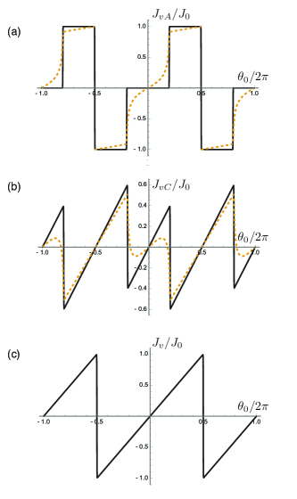
Figure 4: The vacuum current in Andreev and continuum states at $\alpha=0.2$ in the 1D case. Solid lines show currents calculated taking into account only the main terms $\propto 1/L$. Currents calculated taking into account also corrections $\propto 1/L^{3/2}$ at $L/\zeta_{0}=25$ are shown by dashed lines. Here $J_{0}=ev_{f}/L$. (a) The vacuum current $J_{vA}$ in Andreev states. (b) The vacuum current $J_{vC}$ in continuum states. (c) The total vacuum current $J_{v}=J_{vA}+J_{vC}$.

The vacuum current $J_{vA}$ in Andreev states and the continuum vacuum current $J_{vC}$ in the 1D case are shown in Figs. 4(a) and 4(b) respectively. Figure 4(c) shows the total vacuum current $J_{v}=J_{vA}+J_{vC}$. Currents calculated neglecting or taking into account corrections $\propto 1/L^{3/2}$ are shown by solid or dashed lines, respectively. The abrupt jumps of currents produced by the parity effect in the limit $L\to\infty$ are broadened by corrections on the order of $1/L^{3/2}$, which transform them into steep slopes with kinks exactly in the point $\theta_{0}=2\pi\alpha$ Son21 . These jumps and corrections $\propto 1/L^{3/2}$ in the bound states and the continuum compensate each other in the total current, and solid and dashed lines merge. Finally, the plot $J_{v}$ vs. $\theta_{0}$ is the same saw-tooth relation as obtained at $T=0$ (Fig. 2) when the condensate current is the only current in the junction. Finally, the total vacuum current in the 1D case is

$$J_{v}={ev_{f}\over L}{\theta_{0}\over\pi}={en\hbar\over 2m}{\theta_{0}\over L},$$ (56)

where $n=2k_{f}/\pi$ is the 1D electron density.

This picture agrees with calculations at finite $L$ by Bagwell Bagw [see his Fig. 5(a)] Bagwell revealed jumps and kinks of currents in the bound states and in the continuum and their mutual compensation in the total current. But he did not connect them with the parity effect and the incommensurability parameter $\alpha$, which were not considered by him.

Respective contributions of the bound states and the continuum to the total vacuum current depend on dimensionality Son21 . The transition from 1D to multidimensional systems requires averaging of currents over the incommensurability parameter $\alpha$. After averaging the current $J_{vC}$ in continuum states and corrections $\propto 1/L^{3/2}$ both in the bound states and the continuum vanish, and the current $J_{vA}$ in bound states becomes equal to the total current $J_{v}$ described by the saw-tooth relation shown in Fig. 4(c).

For multidimensional systems currents calculated for a single 1D channel must be integrated over the space of wave vectors transverse to the current direction keeping in mind that

$$v_{f}={\hbar k_{f}\over m}={\hbar\sqrt{k_{F}^{2}-k_{\perp}^{2}}\over m},$$ (57)

where $k_{F}$ is the Fermi radius of a multidimensional system and $k_{\perp}$ is a transverse wave vector. The integration operation is $\int_{-k_{F}}^{k_{F}}{dk_{\perp}\over 2\pi}…$ in the 2D case and $\int_{0}^{k_{F}}{k_{\perp}\,dk_{\perp}\over 2\pi}…$ in the 3D case. After integration one obtains that the expression Eq. (56) for the current derived for the 1D case is valid also for multidimensional systems if the 1D electron density $n$ is replaced by the 2D or 3D electron densities.

4.4 Excitation current

For temperatures much higher than the Andreev level energy spacing (small $\beta$), one can replace the sum in Eq. (33) by an integral. Its value yields the excitation current

$$J_{q}=-{ev_{f}\over L}{\theta\over\pi}.$$ (58)

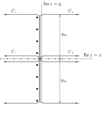
Figure 5: Contour integration in the complex plane $z=x+iy$ for the calculation of the excitation current given by Eq. (33). Small black circles show integer values of $x=s$, which numerate terms of the original sums in Eq. (59). Large black circles show Matsubara poles.

In order to find corrections to this approximate expression we transform the sum in Eq. (33) to

$$J_{q}={2ev_{f}\over L}\left[\sum_{s=0}^{\infty}\frac{1}{e^{\beta\left(s+{\pi+\theta\over 2\pi}\right)}+1}-\sum_{s=-\infty}^{-1}\frac{1}{e^{-\beta\left(s+{\pi+\theta\over 2\pi}\right)}+1}\right].$$ (59)

Next one can use the Matsubara approach transforming the sum to integrals over two contours $C_{+}$ and $C_{-}$ in the complex plane $s=z=x+iy$ shown in Fig. 5:

$$J_{q}={ev_{f}\over iL}\int_{C_{+}}\frac{\cot(\pi z)}{e^{\beta\left(z+{\pi+\theta\over 2\pi}\right)}+1}\,dz+{ev_{f}\over iL}\int_{C_{-}}\frac{\cot(\pi z)}{e^{-\beta\left(z+{\pi+\theta\over 2\pi}\right)}+1}\,dz.$$ (60)

Then we perform analytical continuation transforming the contours $C_{+}$ and $C_{-}$ to the contours $\bar{C}_{+}$ and $\bar{C}_{-}$ (Fig. 5). At this transformation the Matsubara poles on the vertical line $x=-{1\over 2}$,

$$z_{t}=-{1\over 2}-{\theta\over 2\pi}+{2\pi i\over\beta}\left(t+{1\over 2}\right),$$ (61)

are crossed, and the current is

$$J_{q}={ev_{f}\over iL}\left[\int\limits_{\bar{C}_{+}}\frac{\cot(\pi z)}{e^{\beta\left(z+{\pi+\theta\over 2\pi}\right)}+1}\,dz+\int\limits_{\bar{C}_{-}}\frac{\cot(\pi z)}{e^{-\beta\left(z+{\pi+\theta\over 2\pi}\right)}+1}\,dz\right]+\sum_{t=-\infty}^{\infty}M_{t},$$ (62)

where $M_{t}$ is the contribution of the $t$th pole.

Main contributions from contour integrals come from 4 horizontal segments of paths $\bar{C}_{+}$ and $\bar{C}_{-}$. They are integrals over real $x$ at large constant imaginary parts $iy=\pm iy_{m}$. The contribution of the upper segment of contour $\bar{C}_{+}$ is

$${ev_{f}\over iL}\int_{\infty}^{-{1\over 2}}\frac{\cot[\pi(iy_{m}+x)]}{e^{\beta\left(iy_{m}+x+{\pi+\theta\over 2\pi}\right)}+1}\,dx\approx-{ev_{f}\over L}\int_{\infty}^{-{1\over 2}}\frac{dx}{e^{\beta\left(iy_{m}+x+{\pi+\theta\over 2\pi}\right)}+1}$$

$$=\left.{ev_{f}\over L\beta}\ln\left[1+e^{-\beta\left(iy_{m}+x+{\pi+\theta\over 2\pi}\right)}\right]\right\rvert_{x=\infty}^{-{1\over 2}}={ev_{f}\over L\beta}\ln\left[1+e^{-\beta\left(iy_{m}+{\theta\over 2\pi}\right)}\right].$$ (63)

Making similar estimations of other three horizontal segments one obtains the total contribution of all four horizontal segments,

$${ev_{f}\over L\beta}\ln\left\lvert\frac{1+e^{\beta\left(iy_{m}-{\theta\over 2\pi}\right)}}{1+e^{\beta\left(iy_{m}+{\theta\over 2\pi}\right)}}\right\rvert^{2}={ev_{f}\over L\beta}\ln\frac{1+2\cos(\beta y_{m})e^{-{\beta\theta\over 2\pi}}+e^{-{\beta\theta\over\pi}}}{1+2\cos(\beta y_{m})e^{{\beta\theta\over 2\pi}}+e^{{\beta\theta\over\pi}}},$$ (64)

which in the limit $\beta\to 0$ yields the excitation current $J_{q}$ given by Eq. (58). The total contribution of vertical segments of the contours $\bar{C}_{+}$ and $\bar{C}_{-}$ vanishes.

The contribution of the $t$th Matsubara pole is

$$M_{t}={2\pi ev_{f}\over\beta L}\frac{\tan{\theta\over 2}-i\tanh\left[{2\pi^{2}\over\beta}\left(t+{1\over 2}\right)\right]}{1+i\tan{\theta\over 2}\tanh\left[{2\pi^{2}\over\beta}\left(t+{1\over 2}\right)\right]}.$$ (65)

In the high temperature limit $\beta\to 0$ only the poles with $t=0$ and $t=-1$ are important. Finally, the excitation current is

$$J_{q}=-{ev_{f}\over\pi L}\theta+M_{0}+M_{-1}=-{ev_{f}\over\pi L}\theta+{8eT\over\hbar}e^{-2\pi TL/\hbar v_{f}}\sin\theta.$$ (66)

The sinusoidal term in this equation was known before Bard .

Integration over transverse wave vectors in multidimensional systems yields

$$J_{q}=-en{\hbar\over 2m}{\theta\over L}+A_{q}en\sqrt{T\over mk_{F}L}e^{-2\pi TL/\hbar v_{F}}\sin\theta,$$ (67)

where

$$A_{q}=\left\{\begin{array}[]{cc}8{}{}&\mbox{2D case}\\ &\\ 6\pi{}{}&\mbox{3D case}\end{array}\right..$$ (68)

5 Current-phase relation

The current-phase relation is determined by the condition that the sum of the vacuum and the excitation current vanishes. At zero temperature the both current vanish, and the current-phase relation is the saw-tooth curve shown in Fig. 2. In the 1D case at high temperatures the condition imposed by the charge conservation law is

$$J_{v}+J_{q}=en{\hbar\over 2m}{\theta_{0}\over L}-en{\hbar\over 2m}{\theta\over L}+{8eT\over\hbar}e^{-2\pi TL/\hbar v_{f}}\sin\theta$$

$$=-en{\hbar\over 2m}{\theta_{s}\over L}+{8eT\over\hbar}e^{-2\pi TL/\hbar v_{f}}\sin\theta=0.$$ (69)

The current-phase relation is

$$J=J_{s}=en{\hbar\over 2m}{\theta_{s}\over L}={8eT\over\hbar}e^{-2\pi TL/\hbar v_{f}}\sin\theta$$ (70)

for the 1D system, and

$$J=A_{q}en\sqrt{T\over mk_{F}L}e^{-2\pi TL/\hbar v_{F}}\sin\theta$$ (71)

for multidimensional systems. The constant $A_{q}$ is given by Eq. (68).

Because the total current $J$ is exponentially decreases with growing $L$ and $T$, the SNS junction becomes a weak link, and the widely accepted in the past approach neglecting phase gradients in superconducting leads gives the correct result. The phase $\theta_{s}$ connected with phase gradients is small, and the difference between the Josephson phase $\theta=\theta_{0}+\theta_{s}$ and the vacuum phase $\theta_{0}$ is not important. Ignoring $\theta_{s}$ in Eq. (69), the current $J_{v}+J_{q}$ yields a correct value of the total current $J$ despite formal violation of the charge conservation law.

The exponentially small current at high temperature is a result of mutual cancellation of the large terms $\propto 1/L$ in the vacuum current $J_{v}$ and the temperature independent part of the excitation current $J_{q}$. It is not evident that this cancellation is exact. Any power law correction $\propto 1/L^{w}$ independent from temperature becomes more important than the exponentially decaying current at temperatures exceeding the temperature

$$T^{*}={\hbar v_{F}\over 2\pi L}\ln{L\over C},$$ (72)

where the value of $C$ weakly (logarithmically) depends on $T$ and $L$. Due to a large logarithmic factor in Eq. (72), the temperature $T^{*}$ is much larger than the Andreev level energy spacing but, nevertheless, is much smaller than the gap $\Delta_{0}$, and all assumptions made in the calculations are valid.

6 Discussion and conclusions

The present paper investigates the long ballistic SNS junction using the approach initiated in Ref. Son21 . The approach focused on the problem with the charge conservation law in the self-consistent field method dealing with the effective pairing potential that breaks the gauge invariance. This requires to filter solutions obtained by this method keeping only those, which do not violate the charge conservation law. The filtration is provided by the condition that the total currents inside all three layers must be equal. The total current consists of three parts: $J=J_{s}+J_{v}+J_{q}$. The condensate current $J_{s}=env_{s}$ is produced by the phase gradient in the superconducting layers and is the same in all three layers and, therefore, it does not violate the charge conservation law. The vacuum current $J_{v}$ and the excitation current $J_{q}$ flow only in the normal layer, and the charge conservation law requires that $J_{v}+J_{q}=0$. The current-phase relation of the junction is derived from this condition.

At zero temperature the new approach Son21 yielded the same saw-tooth current-phase relation as previous investigations (Fig. 2). But its physical picture was different. In the previous investigations the current $J_{s}$ was ignored, and sloped segments were related only with the vacuum current $J_{v}$ (although the adjective “vacuum” was not used). This was in conflict with the charge conservation law, which requires that the current $J_{v}$ does not flow alone. According to the new approach, slope segments of the curve correspond to the motion of the electron fluid as a whole, and the condensate current $J_{s}$ is the only current in the junction, the value of which is simply derived from the Galilean invariance for Andreev scattering. The calculation of $J_{v}$ using the sophisticated formalism of finite temperature Green’s functions Kulik ; Ishii is not relevant for the current-phase relation at $T=0$. At $T=0$ the electron transport in the SNS junctions does not differ from that in a uniform superconductor.

At nonzero temperatures, one should determine the current-phase relation from the condition $J_{v}+J_{q}=0$, and calculations of two currents $J_{v}$ and $J_{q}$ are necessary. At the calculation of the vacuum current $J_{v}$ in Ref. Son21 the vacuum current in continuum states was neglected. It was correct for multidimensional (2D and 3D) systems, but not for the 1D case. The present paper reports a calculation of the vacuum current in continuum states correcting this error and retracting the prediction of Ref. Son21 that the SNS junction can be a $\varphi_{0}$ junction.

The new calculation of the vacuum current in continuum states showed that the parity effect revealed for the 1D case in Ref. Son21 for the vacuum current in bound states exists also in continuum states. The parity effect produces current jumps and kinks on the current-phase plots. These jumps in bound states and in the continuum are equal in magnitude and opposite in sign, and in the total vacuum current two parity effects compensate each other. In the past current jumps and kinks were revealed in calculations of the current-phase relation in the 1D case by Bagwell Bagw , but their connection with the parity effect was not realized.

One might ask why an essential difference in the physical pictures does not lead to a difference in the outcome of the analysis. This “insensitivity” to the physical picture existed already in the past. The physical pictures of Ishii Ishii and Bardeen and Johnson Bard are not the same. Bardeen and Johnson Bard assumed that the excitation current $J_{q}$ and the condensate current $J_{s}$ derived from the Galilean invariance flow in the normal layer (ignoring that the same current $J_{s}$ flows also in the superconducting layers). Ishii Ishii assumed that the excitation and the vacuum currents $J_{q}$ and $J_{v}$ flow in the normal layer at $T=0$. However, the vacuum current $J_{v}={ev_{f}\over L}{\theta_{0}\over\pi}$ and the condensate current $J_{s}={ev_{f}\over L}{\theta_{s}\over\pi}$ have the same expressions as function of their phases, while the excitation current at high temperatures $J_{q}=-{ev_{f}\over L}{\theta\over\pi}$ (neglecting the exponentially small term from Matsubara poles) has the similar expression via its phase but with an opposite sign. Since Ishii Ishii and Bardeen and Johnson Bard ignored differences between phases $\theta_{0}$ and $\theta$ it did not matter whether $J_{s}$ or $J_{v}$ flows in the normal layer.

Coincidence of the expressions for different currents as functions of their phases takes place in the approximation taking into account only the main terms $\propto 1/L$ and $\propto 1/L^{3/2}$ in the $1/L$ expansion. The agreement with the results of previous works using Ishii or not using Bard the formalism of Green’s functions points out that their results were obtained in the same approximation. The ab initio expressions for different currents are not identical, and the cancellation of temperature independent terms in $J_{v}+J_{q}$ at high temperatures might not retain in a more accurate approximation taking into account terms decreasing with $L$ faster than $1/L^{3/2}$. The estimation of these terms is a subject for a future investigation.

Acknowledgments

Interactions and discussions with Alexander Andreev were very important for my research activity in superfluidity and magnetism. He supported my suggestion of spin superfluidity ES-78b despite it was rejected by some influential Moscow theoreticians. This support was not obtained as granted, and I had to spend a number of nights in the train St. Petersburg (then Leningrad) - Moscow for meetings with Andreev to discuss this issue.

Appendix A Corrections to the contribution of poles in the continuum vacuum current

Let us expand the expression Eq. (45) for residues of poles in $1/L$:

$${\cal R}_{p\pm}\approx{iev_{f}\over 2\pi L}\left[1+{i\zeta_{0}\over L\sqrt{z_{p\pm}(2+z_{p\pm})}}-{\zeta_{0}^{2}\over L^{2}z_{p\pm}(2+z_{p\pm})}\right].$$ (73)

We need only imaginary parts of residues which give real contributions to the current. Using the expressions for coordinates of poles in the complex plane $z=x+iy$ given by Eq. (44) and the inequality $y_{p\pm}\ll x_{p\pm}$ we obtain the correction to the main term $\propto 1/L$:

$$\mbox{Im}\sum_{p}\delta{\cal R}_{p\pm}={ev_{f}\zeta_{0}\over 2\pi L^{2}}\sum_{p}\left[{y_{p\pm}(x_{p\pm}+1)\over(2x_{p\pm}+x_{p\pm}^{2})^{3/2}}-{\zeta_{0}\over L(2x_{p\pm}+x_{p\pm}^{2})}\right]$$

$$={ev_{f}\zeta_{0}^{2}\over 2\pi L^{3}}\sum_{p}\left[{(x_{p\pm}+1)\ln(\sqrt{2x_{p\pm}+x_{p\pm}^{2}}+1+x_{\pm p})\over(2x_{p\pm}+x_{p\pm}^{2})^{3/2}}-{1\over 2x_{p\pm}+x_{p\pm}^{2}}\right].$$ (74)

Terms in the sum smoothly depend on $x_{p\pm}$ without singularities, and one can replace summation by integration over continuous $p$. Since $dp=Ldx_{p\pm}/\pi\zeta_{0}$ the integral is on the order of $1/L^{2}$. But the integral does not depend on $\theta_{0}$ and vanishes in the difference $\mbox{Im}\sum_{p}\delta{\cal R}_{+p}-\mbox{Im}\sum_{p}\delta{\cal R}_{-p}$, which determines the total current of rightmovers and leftmovers. In order to separate the part depending on $\theta_{0}$ one must first to take a derivative in $\theta_{0}$ of any term in the sum first and to replace summation by integration afterwards. Since $d\theta_{0}=2Ldx_{p\pm}/\zeta_{0}$ the $\theta_{0}$ dependent correction is not more than of the order $1/L^{3}$.

Appendix B Calculation of the continuum vacuum current by averaging over transmission oscillations

Here we present another method of calculation of the main term $\propto 1/L$ in the continuum vacuum current, which helps to better understand the role of transmission resonances. We divide the whole interval of integration in the integral Eq. (42) on intervals of the length equal to the oscillation period $\pi\zeta_{0}/L$ of the integrand:

$$J_{\pm}=-{e\Delta_{0}\over\pi\hbar}\left[I_{0}(\gamma_{\pm})+\sum_{p=1}^{p_{m\pm}}I(p,\gamma_{\pm})+I_{m}(\gamma_{\pm})\right],$$ (75)

where

$$I(p,\gamma_{\pm})=\int_{-\pi\zeta_{0}/2L}^{\pi\zeta_{0}/2L}\frac{2\sqrt{2z_{p\pm}+z_{p\pm}^{2}}(1+z_{p\pm})}{4z_{p\pm}+2z_{p\pm}^{2}+1-\cos(2Lz^{\prime}/\zeta_{0})}\,dz^{\prime}={\pi\zeta_{0}\over L}.$$ (76)

Here $z_{p\pm}=x_{p\pm}$ is the real coordinate of the transmission resonance given by Eq. (44), $z^{\prime}=z-z_{p\pm}$, and $p_{m\pm}$ is the maximal integer $p$ satisfying the condition that the upper border of the $p_{m}$th period does not exceed some large $x_{m}$, which in the end must go to infinity:

$$z_{p_{m}\pm}+{\pi\zeta_{0}\over 2L}={(2\pi p_{m\pm}+\pi-\gamma_{\pm})\zeta_{0}\over 2L}<x_{m}.$$ (77)

Inside of any interval we neglected variation of the variable $z$ excepting its variation in the argument of the cosine function. Everywhere else we replace $z$ by its value $z_{p\pm}=x_{p\pm}$ in the interval center, which coincides with location of the $p$th transmission resonance. The sum of terms $I(p,\gamma_{\pm})$ is

$$\sum_{p=1}^{p_{m\pm}}I(p,\gamma_{\pm})={\pi\zeta_{0}\over L}p_{m\pm}.$$ (78)

The term $I_{m}(\gamma_{\pm})$ takes into account the integration interval between the upper limit $x_{m}$ in the integral Eq. (42) and the upper border of the $p_{m\pm}$th period. The integrand at large $z$ goes to 1, and

$$I_{m}(\gamma_{\pm})=x_{m}-z_{p_{m}\pm}-{\pi\zeta_{0}\over 2L}=x_{m}-{(2\pi p_{m\pm}+\pi-\gamma_{\pm})\zeta_{0}\over 2L}.$$ (79)

The term $I_{0}(\gamma_{\pm})$ takes into account the integration interval between $z=0$ and the lower border of the $p=1$ period. In the limit $L\to\infty$ the integrand at small $z$ can be approximated by a delta function:

$$I_{0}(\gamma_{\pm})=\int_{0}^{(\pi-\gamma_{\pm})\zeta_{0}/2L}\frac{2\sqrt{2z}\,dz}{4z+1-\cos(2Lz/\zeta_{0}+\gamma_{\pm})}$$

$$\approx\int_{0}^{(\pi-\gamma_{\pm})\zeta_{0}/2L}{\pi\zeta_{0}\over L}\delta\left(z-{\gamma_{\pm}\zeta_{0}\over 2L}\right)dz={\pi\zeta_{0}\over L}\times\left\{\begin{array}[]{cc}0&\mbox{at}~{}\gamma_{\pm}>0\\ \\ 1&\mbox{at}~{}\gamma_{\pm}<0\end{array}\right..$$ (83)

Substituting the expression for $I_{0}(\gamma_{\pm})$, $\sum\limits_{p=1}^{p_{m\pm}}I(p,\gamma_{\pm})$, and $I_{m}(\gamma_{\pm})$ into Eq. (75) one obtains the value of $J_{\pm}$ identical to the term $\propto 1/L$ in Eq. (54).

References

- \bibcommenthead
- (1) Andreev, A.F.: The thermal conductivity of the intermediate state in superconductors. Zh. Eksp. Teor. Fiz. 46, 1823–1828 (1964). [Sov. Phys.–JETP, 19, 1228–1231 (1964)]
- (2) Lifshitz, E.M., Pitaevskii, L.P.: Absorption of second sound in rotating helium II. Zh. Eksp. Teor. Fiz. 33, 535–537 (1957). [Sov. Phys.–JETP, 6, 418–419 (1958)]
- (3) Sonin, E.B.: Friction between the normal component and vortices in rotating superfluid helium. Zh. Eksp. Teor. Fiz. 69, 921–935 (1975). [Sov. Phys.–JETP, 42, 469–475 (1976)]
- (4) Gal’perin, Y.M., Sonin, E.B.: Motion of vortices and electrical conductivity of pure type II supercomductors in weak magnetic fields. Fiz. Tverd. Tela (Leningrad) 18, 3034–3041 (1976). [Sov. Phys.–Solid State, 18, 1768–1772 (1976)]
- (5) Kopnin, N.B., Kravtsov, V.E.: Forces acting on vortices moving in a pure type II superconductor. Zh. Eksp. Teor. Fiz. 71, 1644–1656 (1976). [Sov. Phys.–JETP, 44, 861–867 (1976)].
- (6) Sonin, E.B.: Dynamics of Quantised Vortices in Superfluids. Cambridge University Press, Cambridge (2016)
- (7) Tsepelin, V., Baggaley, A.W., Sergeev, Y.A., Barenghi, C.F., Fisher, S.N., Pickett, G.R., Jackson, M.J., Suramlishvili, N.: Visualization of quantum turbulence in superfluid 3He-: Combined numerical and experimental study of Andreev reflection. Phys. Rev. B 96, 054510 (2017). https://doi.org/10.1103/PhysRevB.96.054510
- (8) Skrbek, L., Sergeev, Y.A.: Feasibility of an analog of Andreev reflection in superfluid . Phys. Rev. B 108, 100502 (2023). https://doi.org/10.1103/PhysRevB.108.L100502
- (9) Andreev, A.F.: Electron spectrum of the intermediate state of superconductors. Zh. Eksp. Teor. Fiz. 49, 655–660 (1964). [Sov. Phys.–JETP, 22, 455–458 (1966)]
- (10) Kulik, I.O.: Macroscopic quantization and proxity effect in S–N–S junctions. Zh. Eksp. Teor. Fiz. 57, 1745–1759 (1969). [Sov. Phys.–JETP, 30, 944–950 (1970)]
- (11) Ishii, C.: Josephson currents through junctions with normal metal barriers. Prog. Theor. Phys. (Japan) 44, 1525–1546 (1970)
- (12) Bardeen, J., Johnson, J.L.: Josephson current flow in pure Superconducting-Normal-Superconducting junctions. Phys. Rev B 5, 72–78 (1972)
- (13) de Gennes, P.G.: Superconductivity of Metals and Alloys. Benjamin, New York (1966)
- (14) Thuneberg, E.: Comment on “Ballistic SNS sandwich as a Josephson junction”. Phys. Rev. B 108, 176501 (2023)
- (15) Sonin, E.B.: Ballistic SNS sandwich as a Josephson junction. Phys. Rev. B 104, 094517 (2021)
- (16) Riedel, R.A., Chang, L.-F., Bagwell, P.F.: Critical current and self-consistent order parameter of a superconductor–normal-metal–superconductor junction. Phys. Rev. B 54, 16082–16095 (1996). https://doi.org/10.1103/PhysRevB.54.16082
- (17) Sols, F., Ferrer, J.: Crossover from the Josephson effect to bulk superconducting flow. Phys. Rev. B 49, 15913–15919 (1994). https://doi.org/10.1103/PhysRevB.49.15913
- (18) Davydova, M., Prembabu, S., Fu, L.: Universal Josephson diode effect. Sci. Adv. 8(23) (2022). https://doi.org/10.1126/sciadv.abo0309
- (19) Sonin, E.B.: Reply to Comment on “Ballistic SNS sandwich as a Josephson junction”. Phys. Rev. B 108, 176502 (2023)
- (20) Buzdin, A.: Direct coupling between magnetism and superconducting current in the Josephson junction. Phys. Rev. Lett. 101, 107005 (2008). https://doi.org/10.1103/PhysRevLett.101.107005
- (21) Svidzinskii, A.V., Antsygina, T.N., Bratus, E.N.: Superconducting current in wide S–N–S junctions. Zh. Eksp. Teor. Fiz. 61, 1612–1619 (1971). [Sov. Phys.–JETP, 34, 860–863 (1972)]
- (22) Gunsenheimer, U., Schüssler, U., Kümmel, R.: Symmetry breaking, off-diagonal scattering, and Josephson currents in mesoscopic weak links. Phys. Rev. B 49, 6111–6125 (1994). https://doi.org/10.1103/PhysRevB.49.6111
- (23) Tinkham, M.: Introduction to Superconductivity, 2nd edn. McGrow-Hill, New York (1996)
- (24) Bagwell, P.F.: Suppression of the Josephson current through a narrow, mesoscopic, semiconductor channel by a single impurity. Phys. Rev. B 46, 12573–12586 (1992). https://doi.org/10.1103/PhysRevB.46.12573
- (25) Gradshteyn, I.S., Ryzhik, I.M.: Table of Integrals, Series, and Products, 7th edn. Academic Press, Amsterdam (2007)
- (26) Sonin, E.B.: Analogs of superfluid currents for spins and electron-hole pairs. Zh. Eksp. Teor. Fiz. 74, 2097–2111 (1978). [Sov. Phys.–JETP, 47, 1091–1099 (1978)]