A New Two-Sided Sketching Algorithm for Large-Scale Tensor Decomposition Based on Discrete Cosine Transformation

Abstract

Large tensors are frequently encountered in various fields such as computer vision, scientific simulations, sensor networks, and data mining. However, these tensors are often too large for convenient processing, transfer, or storage. Fortunately, they typically exhibit a low-rank structure that can be leveraged through tensor decomposition. Despite this, performing large-scale tensor decomposition can be time-consuming. Sketching is a useful technique to reduce the dimensionality of the data. In this study, we introduce a novel two-sided sketching method based on the $t$-product decomposition and the discrete cosine transformation. We conduct a thorough theoretical analysis to assess the approximation error of the proposed method. Specifically, we enhance the algorithm with power iteration to achieve more precise approximate solutions. Extensive numerical experiments and comparisons on low-rank approximation of color images and grayscale videos illustrate the efficiency and effectiveness of the proposed approach in terms of both CPU time and approximation accuracy.

Key words. Large-scale tensor, tensor decomposition, sketching, $t$-product, discrete cosine transformation, power iteration.

1 Introduction

Multidimensional arrays, known as tensors, are often used to represent real-world high-dimensional data, such as videos [1, 2], hyperspectral images [3, 4, 5, 6], multilinear signals [7, 8], and communication networks [9, 10]. In most cases, these tensor data usually have a low-rank structure and can be approximated by tensor decomposition. Nevertheless, computing the tensor decomposition of these large-scale data is usually computationally demanding, and thus finding an accurate approximation of large-scale data with great efficiency plays a key role in tensor data analysis. Sketching is a useful technique for data compression, utilizing random projections or sampling to imitate the original data. Although the sketching technique may slightly reduce the accuracy of the approximation, it can significantly reduce the computational and storage complexity [15]. As a result, sketching is commonly used in low-rank tensor approximation, and many researchers have proposed various tensor sketching algorithms [17, 18, 19, 20, 21, 22, 23, 24, 25, 26, 27]. They have also been successfully applied to a variety of tasks, such as Kronecker product regression, polynomial approximation, and the construction of deep convolutional neural networks [29, 30, 31, 32, 33, 34], etc.

Recently, extensive research has been carried out on the application of sketching algorithms for low-rank matrix approximation [35, 36, 37, 38]. Woodruff et al. [36] examined the numerical linear algebra algorithms of linear sketching techniques and identified their limitations. Tropp et al. [37] developed the two-sided matrix sketching algorithm, which can maintain the structural properties of the input matrix and generate a low-rank matrix approximation with a given rank. Tropp et al. [38] also proposed a new two-sided matrix sketching algorithm to construct a low-rank approximation matrix from streaming data. These matrix sketching algorithms are very effective in reducing storage and computational costs when computing low-rank approximations of large-scale matrices. Subsequently, many researchers have applied matrix sketching algorithms to tensor decomposition and developed various low-rank tensor approximation algorithms. The following are some low-rank tensor approximation algorithms based on different decompositions [16, 17, 18, 19, 20, 21, 22, 23, 24, 25, 26, 27, 28].

Based on the CANDECOMP/PARAFAC (CP) decomposition, the robust tensor power method based on tensor sketch (TS-RTPM) can quickly mine the potential features of tensor, but in some cases, its approximation performance is limited, Cao et al. [16] propose a data-driven framework called TS-RTPM-Net, which improves the estimation accuracy of TS-RTPM by jointly training the TS value matrices with the RTPM initial matrices. Li et al. [17] introduced a randomized algorithm for CP tensor decomposition in least squares regression, aiming to achieve reduced dimensionality and sparsity in the randomized linear mapping. Wang et al. [18] developed innovative techniques for performing randomized tensor contractions using FFTs, avoiding the explicit formation of tensors. Numerous studies have also been conducted based on Tucker decomposition [19, 20, 21, 22, 23, 24, 27, 28]. For instance, Che et al. [19] devised an adaptive randomized approach for approximating Tucker decomposition. Malik et al. [22] proposed two randomized algorithms for low-rank Tucker decomposition, which entail a single pass of the input tensor by integrating sketching. Ravishankar et al. [23] introduced the hybrid Tucker TensorSketch vector quantization (HTTSVQ) algorithm for dynamic light fields. Sun et al. [24] developed a randomized method for Tucker decomposition, which can provide a satisfactory approximation of the original tensor data through the incorporation of two-sided sketching. Minster et al. [27] devised randomized adaptations of the THOSVD and STHOSVD algorithms. Dong et al. [28] present two practical randomized algorithms for low-rank Tucker approximation of large tensors based on sketching and power scheme, with a rigorous errorbound analysis. The work based on tensor-train (TT) decomposition can be found e.g. in [19, 25, 39, 40]. In particular, Che et al. [19] designed an adaptive random algorithm to calculate the tensor column approximation. Hur et al. [25] introduced a sketching algorithm to construct a TT representation of a probability density from its samples, which can avoid the curse of dimensionality and sample complexities of the recovery problem. Qi and Yu [26] proposed a tensor sketching method based on the $t$-product, which can quickly obtain a low tubal rank tensor approximation. As pointed out by Kernfeld et al. [41], the $t$-product has a disadvantage in that, for real tensors, implementation of the $t$-product and factorizations using the $t$-product require intermediate complex arithmetic, which, even taking advantage of complex symmetry in the Fourier domain, is more expensive than real arithmetic.

In this paper, based on the $\star_{L}$-product decomposition [41], we investigate some new two-sided sketching algorithms for low tubal rank tensor approximation. The main contributions of this paper are twofold. Firstly, we propose a new one-pass sketching algorithm (i.e., Algorithm 1), which can significantly improve the computational efficiency of T-sketch and rt_SVD, for low tubal rank approximation. Secondly, we first establish a low tubal rank tensor approximation model based on $\star_{L}-$product factorization, extending the two-sided matrix sketching algorithm proposed by Tropp et al. [38]. A rigorous theoretical analysis is conducted to evaluate the approximation error of the proposed DCT Gaussian-Sketch PI algorithm.

The following paper is organized as follows. Section 2 introduces some common notations and preliminaries. Section 3 presents two-sided sketching algorithms based on the transformed domain (i.e., Algorithm 1, Algorithm 2). Section 4 provides strict theoretical guarantees for the approximation error of the proposed algorithms. Section 5 presents numerical experiments and comparisons demonstrating the efficiency and effectiveness of the proposed algorithms. We conclude in Section 6.

2 Notations and Preliminaries

In this paper, matrices and tensors are represented by capital letters (e.g. $A,B,\dots$) and curly letters (e.g. $\mathcal{A},\mathcal{B},\dots$), respectively. We can use the Matlab command $A^{\prime}$ represent conjugate transpose of the matrix $A$. $\mathbb{R}$ and $\mathbb{C}$ represent the real number space and the complex number space, respectively. For matrix $A\in\mathbb{C}^{n_{1}\times n_{2}}$, its $(i,j)$-th element is represented by $a_{i,j}$. For third-order tensor $\mathcal{A}\in\mathbb{C}^{n_{1}\times n_{2}\times n_{3}}$, its $(i,j,k)$-th element is represented by $a_{i,j,k}$. The Matlab notations $\mathcal{A}(i,:,:)$, $\mathcal{A}(:,i,:)$ and $\mathcal{A}(:,:,i)$ are used to represent the $i$-th horizontal, lateral and facial slices of $\mathcal{A}$, respectively. The facial slice $\mathcal{A}(:,:,i)$ is also represented by $\mathcal{A}^{(i)}$. The Frobenius norm of a tensor is defined as the square root of the sum of the squares of its elements:

$${\|\mathcal{A}\|}_{F}:={\|\mathcal{A}(:)\|}_{2}=\sqrt{\langle{\mathcal{A},\mathcal{A}}\rangle}=\sqrt{\sum_{ijk}|a_{ijk}|^{2}}\ .$$ (2.1)

$\mathcal{A}^{H}$ and $\mathcal{A}^{\dagger}$ represent the conjugate transpose and pseudo-inverse of $\mathcal{A}$, respectively.

This paper focuses on the low tubal rank tensor approximation meeting desired accuracy in an efficient manner. For tensor $\mathcal{A}\in\mathbb{R}^{n_{1}\times n_{2}\times n_{3}}$, the mathematical model for finding the low-rank approximation $\hat{\mathcal{A}}$ of $\mathcal{A}$ can be expressed as

$${\|\mathcal{A}-\hat{\mathcal{A}}\|}_{F}=\min_{{\rm rank}_{L}(\mathcal{B})\leq l}{\|\mathcal{A}-\mathcal{B}\|}_{F},$$ (2.2)

where $l$, $l\ll\min\{n_{1},n_{2}\}$, is the target rank, $L$ (by abuse of notation) represents an arbitrary invertible linear transform, and ${\rm rank}_{L}(\mathcal{B})$ denotes the transformed tubal rank of tensor $\mathcal{B}$.

2.1 Transformed Tensor SVD

We below briefly recall the transformed tensor SVD of third-order tensors; more details can be found in [41, 46].

Let $F_{n_{3}}$ and $C_{n_{3}}$ represent the discrete Fourier transform matrix and the DCT matrix, respectively. For any third-order tensor $\mathcal{A}\in\mathbb{R}^{n_{1}\times n_{2}\times n_{3}}$, let $\bar{\mathcal{A}}_{L}$ represent a third-order tensor obtained via multiplied by $L$ (an arbitrary invertible linear transform) on all tubes along the third-dimension of $\mathcal{A}$, i.e., $\bar{\mathcal{A}}_{L}(i,j,:)=L(\mathcal{A}(i,j,:))$, $i=1,\dots,n_{1},j=1,\dots,n_{2}$. Here we write $\bar{\mathcal{A}}_{L}=L[\mathcal{A}]$. Moreover, one can get $\mathcal{A}$ from $\bar{\mathcal{A}}_{L}$ by using $L^{H}$ along the third-dimension of $\bar{\mathcal{A}}_{L}$, i.e., $\mathcal{A}=L^{H}[\bar{\mathcal{A}}_{L}]$. The $\star{{}_{L}}$-product is defined in Definition 2.1 below.

Definition 2.1

[41] For any two tensors $\mathcal{X}\in\mathbb{C}^{n_{1}\times n_{2}\times n_{3}}$ and $\mathcal{Y}\in\mathbb{C}^{n_{2}\times n_{4}\times n_{3}}$, and an arbitrary invertible linear transform $L$, the $\star{{}_{L}}$-product of $\mathcal{X}$ and $\mathcal{Y}$ is a tensor $\mathcal{Z}\in\mathbb{C}^{n_{1}\times n_{4}\times n_{3}}$ given by

$$\mathcal{Z}=\mathcal{X}\star{{}_{L}}\mathcal{Y}=L^{H}[\text{fold}(\text{Block}(\bar{\mathcal{X}}_{L})\text{Block}(\bar{\mathcal{Y}}_{L}))],$$ (2.3)

where $\text{fold}(\text{Block}(\bar{\mathcal{X}}_{L}))=\bar{\mathcal{X}}_{L}$ and $\bar{X}_{L}=\text{Block}(\bar{\mathcal{X}}_{L})=\begin{pmatrix}\bar{\mathcal{X}}_{L}^{(1)}&&&\\ &\bar{\mathcal{X}}_{L}^{(2)}&&\\ &&\ddots&\\ &&&\bar{\mathcal{X}}_{L}^{(n_{3})}\end{pmatrix}$.

Definition 2.2

The Kronecker product of matrices $A\in\mathbb{C}^{m\times l}$ and $B\in\mathbb{C}^{p\times r}$ is

$$A\otimes B=\begin{pmatrix}a_{11}B&a_{12}B&\dots&a_{1l}B\\ a_{21}B&a_{22}B&\ddots&a_{2l}B\\ \vdots&\vdots&\ddots&\vdots\\ a_{m1}B&a_{m2}B&\dots&a_{ml}B\end{pmatrix}.$$

The $t$-product [47] of $\mathcal{A}\in\mathbb{C}^{n_{1}\times n_{2}\times n_{3}}$ and $\mathcal{B}\in\mathbb{C}^{n_{2}\times n_{4}\times n_{3}}$ is a tensor $\mathcal{C}\in\mathbb{C}^{n_{1}\times n_{4}\times n_{3}}$ given by

$$\begin{split}\mathcal{C}=\mathcal{A}*\mathcal{B}=\text{Fold}_{\text{vec}}(\text{Circ}(\mathcal{A})\times\text{Vec}(\mathcal{B})),\end{split}$$ (2.4)

where

$$\text{Vec}(\mathcal{B})=\begin{pmatrix}\mathcal{B}^{(1)}\\ \mathcal{B}^{(2)}\\ \vdots\\ \mathcal{B}^{(n_{3})}\end{pmatrix}\in\mathbb{R}^{n_{2}n_{3}\times n_{4}},\quad\text{Fold}_{\text{vec}}(\text{Vec}(\mathcal{B}))=\mathcal{B},$$

$$\text{Circ}(\mathcal{A})=\begin{pmatrix}\mathcal{A}^{(1)}&\mathcal{A}^{(n_{3})}&\mathcal{A}^{(n_{3}-1)}&\dots&\mathcal{A}^{(2)}\\ \mathcal{A}^{(2)}&\mathcal{A}^{(1)}&\mathcal{A}^{(n_{3})}&\dots&\mathcal{A}^{(3)}\\ \vdots&\vdots&\vdots&\ddots&\vdots\\ \mathcal{A}^{(n_{3})}&\mathcal{A}^{(n_{3}-1)}&\mathcal{A}^{(n_{3}-2)}&\dots&\mathcal{A}^{(1)}\end{pmatrix}.$$

The $t$-product in Eq. (2.4) can be seen as a special case of Definition 2.1. Recall that the block circulant matrix $\text{Circ}(\mathcal{A})$ can be diagonalized by the fast Fourier transform matrix $F_{n_{3}}$ and the block diagonal matrices are the frontal slices of $\bar{\mathcal{A}}_{\text{$F_{n_{3}}$}}$ ,i.e.,

$$(\text{$F_{n_{3}}$}\otimes I_{n_{1}})\times\text{Circ}(\mathcal{A})\times(\text{$F^{H}_{n_{3}}$}\otimes I_{n_{2}})=\text{Block}(\bar{\mathcal{A}}_{\text{$F_{n_{3}}$}})=\bar{A}_{\text{$F_{n_{3}}$}}.$$

It follows that

$$\mathcal{A}*\mathcal{B}=\text{Fold}_{\text{vec}}(\text{Circ}(\mathcal{A})\times\text{Vec}(\mathcal{B}))$$

$$= \text{Fold}_{\text{vec}}((\text{$F^{H}_{n_{3}}$}\otimes I_{n_{1}})\times\text{Block}(\bar{\mathcal{A}}_{\text{$F_{n_{3}}$}})\times(\text{$F_{n_{3}}$}\otimes I_{n_{2}})\times\text{Vec}(\mathcal{B}))$$

$$= \text{fold}((\text{$F^{H}_{n_{3}}$}\otimes I_{n_{1}})\times\text{Block}(\bar{\mathcal{A}}_{\text{$F_{n_{3}}$}})\times\text{Block}(\bar{\mathcal{B}}_{\text{$F_{n_{3}}$}}))$$

$$= \text{$F^{H}_{n_{3}}$}[\text{fold}(\text{Block}(\bar{\mathcal{A}}_{\text{$F_{n_{3}}$}})\text{Block}(\bar{\mathcal{B}}_{\text{$F_{n_{3}}$}}))]$$

$$= \text{$F^{H}_{n_{3}}$}[\text{fold}(\bar{A}_{\text{$F_{n_{3}}$}}\bar{B}_{\text{$F_{n_{3}}$}})]$$

$$= \mathcal{A}\star_{\text{$F_{n_{3}}$}}\mathcal{B}.$$

The definitions of the conjugate transpose of tensor, the identity tensor, the unitary tensor, the invertible tensor, the diagonal tensor, and the inner product between two tensors related to the $\star{{}_{L}}$-product are given as follows.

• [46] The conjugate transpose of $\mathcal{A}\in\mathbb{C}^{n_{1}\times n_{2}\times n_{3}}$ with respect to $L$ is the tensor $\mathcal{A}^{H}\in\mathbb{C}^{n_{1}\times n_{2}\times n_{3}}$ obtained by $\mathcal{A}^{H}=L^{H}[\text{fold}(\text{Block}(\bar{\mathcal{A}}_{L})^{H})]=L^{H}[\text{fold}(\bar{A}^{H}_{L})].$

• [41] The identity tensor $\mathcal{I}_{L}\in\mathbb{C}^{n\times n\times n_{3}}$ (with respect to $L$) is defined to be a tensor such that $\mathcal{I}_{L}=L^{H}[\mathcal{I}]$, where $\mathcal{I}$ with each frontal slice being the $n\times n$ identity matrix.

• [41] A tensor $\mathcal{Q}\in\mathbb{C}^{n\times n\times n_{3}}$ is unitary with respect to $\star{{}_{L}}$-product if it satisfies ${\mathcal{Q}^{H}}\star{{}_{L}}\mathcal{Q}=\mathcal{Q}\star{{}_{L}}\mathcal{Q}^{H}=\mathcal{I}_{L}$, where $\mathcal{I}_{L}$ is the identity tensor.

• [41] For tensors $\mathcal{A}\in\mathbb{C}^{n\times n\times n_{3}},\mathcal{B}\in\mathbb{C}^{n\times n\times n_{3}}$, if ${\mathcal{A}}\star{{}_{L}}\mathcal{B}=\mathcal{B}\star{{}_{L}}\mathcal{A}=\mathcal{I}_{L}$, then tensor $\mathcal{B}$ is the invertible tensor under the $\star{{}_{L}}$-product of tensor $\mathcal{A}$.

• [47] A tensor is a diagonal tensor if each frontal slice of the tensor is a diagonal matrix. For a third-order tensor, if all of its frontal slices are upper or lower triangles, then the tensor is called f-upper or f-lower.

Lemma 2.3

[41, 47] Suppose that $\mathcal{A}\in\mathbb{R}^{m\times k\times p}$ and $\mathcal{B}\in\mathbb{R}^{k\times n\times p}$ are two arbitrary tensors. Let $\mathcal{Z}=\mathcal{X}\star{{}_{L}}\mathcal{Y}$. Then the following properties hold:

• ${{\|\mathcal{A}\|}_{F}^{2}}=\frac{1}{p}{\|\bar{A}_{\text{$F_{n_{3}}$}}\|}_{F}^{2}=\frac{1}{p}{\|\bar{A}_{L}\|}_{F}^{2}=\frac{1}{p}\sum_{i=1}^{p}{\|\bar{\mathcal{A}}^{(i)}_{L}\|}_{F}^{2}$.

• $\mathcal{Z}=\mathcal{X}\star{{}_{L}}\mathcal{Y}$ is equivalent to $\text{Block}(\bar{\mathcal{Z}}_{L})=\text{Block}(\bar{\mathcal{A}}_{L})\text{Block}(\bar{\mathcal{B}}_{L})$$(i.e.,\bar{Z}_{L}=\bar{A}_{L}\bar{B}_{L})$.

Definition 2.4

(Gaussian random tensor) [48] A tensor $\mathcal{G}\in\mathbb{R}^{m\times n\times p}$ is called a Gaussian random tensor if the elements of $\mathcal{G}^{(1)}$ satisfy the standard normal distribution (i.e., Gaussian with mean zero and variance one) and the other frontal slices are all zero.

Based on the above definitions, we have the following transformed tensor SVD with respect to $L$.

Theorem 2.5

[41] For any $\mathcal{A}\in\mathbb{C}^{n_{1}\times n_{2}\times n_{3}}$, the transformed tensor SVD is given by

$$\mathcal{A}=\mathcal{U}\star{{}_{L}}\mathcal{S}\star{{}_{L}}\mathcal{V}^{H},$$ (2.5)

where $\mathcal{U}\in\mathbb{C}^{n_{1}\times n_{1}\times n_{3}}$ and $\mathcal{V}\in\mathbb{C}^{n_{2}\times n_{2}\times n_{3}}$ are unitary tensors with respect to the $\star{{}_{L}}$-product, and $\mathcal{S}\in\mathbb{C}^{n_{1}\times n_{2}\times n_{3}}$ is diagonal.

The transformed tubal rank, denoted as ${\rm rank}_{L}(\mathcal{A})$, is defined as the number of nonzero singular tubes of $\mathcal{S}$, where $\mathcal{S}$ comes from the transformed tensor SVD of $\mathcal{A}=\mathcal{U}\star{{}_{L}}\mathcal{S}\star{{}_{L}}\mathcal{V}^{H}$, i.e.,

$$\begin{split}{\rm rank}_{L}(\mathcal{A})=\#\{i:\mathcal{S}(i,i,:)\neq 0\},\end{split}$$ (2.6)

where # denotes the cardinality of a set. The transformed tensor SVD could be implemented efficiently by the SVDs of the frontal slices in the transformed domain. We also refer the readers to [46] for more details about the computation of the transformed tensor SVD.

For the Kernfeld-Kilmer transformed tensor SVD (i.e., Eq. (2.5)), by [41, 47, 49], we have

$$\sum_{k=1}^{p}\mathcal{S}(1,1,k)^{2}\geq\sum_{k=1}^{p}\mathcal{S}(2,2,k)^{2}\geq\dots\geq\sum_{k=1}^{p}\mathcal{S}(\min\{m,n\},\min\{m,n\},k)^{2}.$$ (2.7)

Definition 2.6

(Transformed Tensor Singular Values) Suppose $\mathcal{A}\in\mathbb{R}^{m\times n\times p}$ with a Kernfeld-Kilmer transformed tensor SVD such that Eq. (2.7) is satisfied. The $i$-th largest transformed tensor singular value of $\mathcal{A}$ is defined as

$$\sigma_{i}=\sqrt{\sum_{k=1}^{p}\mathcal{S}(i,i,k)^{2}},\quad{\rm for}\ i=1,2,\dots,\min\{m,n\}.$$ (2.8)

Similarly to the definition of the matrix tail energy, the tail energy of tensor is defined below.

Definition 2.7

(Tail Energy) For tensor $\mathcal{A}\in\mathbb{R}^{m\times n\times p}$, the $i$-th largest transformed tensor singular value is $\sigma_{i}$, $i=1,\dots,\min\{m,n\}$. Then the $j$-th tail energy of $\mathcal{A}$ is defined as

$${\tau_{j}}^{2}(\mathcal{A}):=\min_{{\rm rank}_{L}(\mathcal{B})<j}{\|\mathcal{A}-\mathcal{B}\|}_{F}^{2}=\sum_{i\geq j}\sigma_{i}^{2}(\mathcal{A}).$$ (2.9)

According to the above definition and using Lemma 2.3 and the linearity, we can obtain

$${\tau_{j}}^{2}(\mathcal{A}) = \sum_{i\geq j}\sigma_{i}^{2}(\mathcal{A})=\sum_{i\geq j}{\|\mathcal{A}_{i}-\mathcal{A}_{i-1}\|}_{F}^{2}$$

$$= \sum_{i\geq j}\frac{1}{p}\sum_{k=1}^{p}{\|\bar{\mathcal{A}}_{(i)_{L}}-\bar{\mathcal{A}}_{{(i-1)}_{L}}\|}_{F}^{2}$$

$$= \frac{1}{p}\sum_{i=1}^{p}{\tau_{j}}^{2}(\bar{\mathcal{A}}_{L}^{(i)}),$$

where $\bar{\mathcal{A}}_{(i)_{L}}$ represents a third-order tensor obtained via being multiplied by $L$ on all tubes along the third-dimension of $\mathcal{A}_{(i)}$. We then have the following proposition.

Proposition 2.8

Suppose $\mathcal{A}\in\mathbb{R}^{m\times n\times p}$ and $\bar{\mathcal{A}}_{L}$ represents a third-order tensor obtained via being multiplied by $L$ on all tubes along the third-dimension of $\mathcal{A}$. Let $j$ be a positive integer satisfying $j\leq\min\{m,n\}$. Then

$${\tau_{j}}^{2}(\mathcal{A})=\frac{1}{p}\sum_{i=1}^{p}{\tau_{j}}^{2}(\bar{\mathcal{A}}_{L}^{(i)}).$$ (2.10)

2.2 Tensor Sketching Operator

Using the three matrix sketching operators introduced in the Appendix A, three corresponding tensor sketching operators can be generated. As for a new two-sided sketching algorithm, we need to generate four random linear dimension reduction maps, i.e.,

$$\Upsilon\in\mathbb{R}^{k\times m\times p},\ \ \Omega\in\mathbb{R}^{k\times n\times p},\ \ \displaystyle\Phi\in\mathbb{R}^{s\times m\times p},\ \ {\rm and}\ \Psi\in\mathbb{R}^{s\times n\times p}.$$ (2.11)

Different ways of generating tensor sketch operators are shown below.

• Gaussian tensor sketching operator. Set
  $\Upsilon=\text{zeros}(k,m,p);\ \Upsilon(:,:,1)=\texttt{GaussianProjection}(\mathcal{A}(:,:,1),k)^{\prime}$;
  $\Omega=\text{zeros}(k,n,p);\ \Omega(:,:,1)=\texttt{GaussianProjection}(\mathcal{A}(:,:,1)^{\prime},k)^{\prime};\\ \Phi=\text{zeros}(s,m,p);\ \Phi(:,:,1)=\texttt{GaussianProjection}(\mathcal{A}(:,:,1),s)^{\prime}$;
  $\Psi=\text{zeros}(s,n,p);\ \Psi(:,:,1)=\texttt{GaussianProjection}(\mathcal{A}(:,:,1)^{\prime},s)^{\prime}$.
  Then $\Upsilon$, $\Omega$, $\Phi$ and $\Psi$ are said to be Gaussian tensor sketching operators.

• SRHT tensor sketching operator. Set
  $\Upsilon=\text{zeros}(k,m,p);\ \Upsilon(:,:,1)=\texttt{SRHT}(\mathcal{A}(:,:,1),k)^{\prime}$;
  $\Omega=\text{zeros}(k,n,p);$  $\Omega(:,:,1)=\texttt{SRHT}(\mathcal{A}(:,:,1)^{\prime},k)^{\prime};\\ \Phi=\text{zeros}(s,m,p);\ \Phi(:,:,1)=\texttt{SRHT}(\mathcal{A}(:,:,1),s)^{\prime}$;
  $\Psi=\text{zeros}(s,n,p);\ \Psi(:,:,1)=\texttt{SRHT}(\mathcal{A}(:,:,1)^{\prime},s)^{\prime}$.
  Then $\Upsilon$, $\Omega$, $\Phi$ and $\Psi$ are said to be SRHT tensor sketching operators.

• Count tensor sketching operator. For $i=1,2,\ldots,p$, set
  $\Upsilon=\text{zeros}(k,m,p);\ \Upsilon(:,:,i)=\texttt{CountSketch}(\mathcal{A}(:,:,1),k)^{\prime}$;
  $\Omega=\text{zeros}(k,n,p);\ \Omega(:,:,i)=\texttt{CountSketch}(\mathcal{A}(:,:,1)^{\prime},k)^{\prime};\\ \Phi=\text{zeros}(s,m,p);\ \Phi(:,:,i)=\texttt{CountSketch}(\mathcal{A}(:,:,1),s)^{\prime}$;
  $\Psi=\text{zeros}(s,n,p);\ \Psi(:,:,i)=\texttt{CountSketch}(\mathcal{A}(:,:,1)^{\prime},s)^{\prime}$.
  Then $\Upsilon$, $\Omega$, $\Phi$ and $\Psi$ are said to be count tensor sketching operators.

3 Two-Sided Sketching Algorithms Based on the Transformed Domain

Qi and Yu[26] proposed the two-sided tensor sketching algorithm that only considers range and co-range of the input tensor. On this basis, we also consider the core sketch. The core sketch contains new information that improves our estimates of the transformed tensor singular values and the transformed tensor singular vectors of the input tensor and is responsible for the superior performance of the algorithms. Therefore, We present the framework of our new two-sided sketching algorithm for low tubal rank tensor approximation.

Given the input tensor $\mathcal{A}\in\mathbb{R}^{m\times n\times p}$ and the objective tubal rank $k$, using the appropriate tensor sketching operators in Eq. (2.11), we may realize the randomized sketches $(\mathcal{X},\mathcal{Y},\mathcal{Z})$ such as

$$\mathcal{X}:=\Upsilon\star{{}_{L}}\mathcal{A}\in\mathbb{R}^{k\times n\times p},\quad\mathcal{Y}:=\mathcal{A}\star{{}_{L}}{\Omega}^{H}\in\mathbb{R}^{m\times k\times p};$$ (3.12)

$$\mathcal{Z}:=\Phi\star{{}_{L}}\mathcal{A}\star{{}_{L}}\Psi^{H}\in\mathbb{R}^{s\times s\times p}.$$ (3.13)

The first two tensor sketches $\mathcal{X}$ and $\mathcal{Y}$ capture the co-range and range of $\mathcal{A}$, respectively. The core sketch $\mathcal{Z}$ contains new information that improves our estimates of the transformed tensor singular values and the transformed tensor singular vectors of $\mathcal{A}$ and is responsible for the superior performance of the algorithms.

Once the sketches $(\mathcal{X},\mathcal{Y},\mathcal{Z})$ of the input tensor $\mathcal{A}$ are obtained, we can find the low-rank approximation $\hat{\mathcal{A}}$ by following a three-step process below.

1. Form an L-orthogonal-triangular factorization

$$\mathcal{X}^{H}:=\mathcal{P}\star{{}_{L}}\mathcal{R}_{1},\quad\mathcal{Y}:=\mathcal{Q}\star{{}_{L}}\mathcal{R}_{2},$$ (3.14)

where $\mathcal{P}\in\mathbb{R}^{n\times k\times p}$ and $\mathcal{Q}\in\mathbb{R}^{m\times k\times p}$ are partially orthogonal tensors, and $\mathcal{R}_{1}\in\mathbb{R}^{k\times k\times p}$ and $\mathcal{R}_{2}\in\mathbb{R}^{k\times k\times p}$ are f-upper triangular tensors, in the sense of the $\star{{}_{L}}$-product operation.

2. Solve the least-squares problem based on $\star{{}_{L}}$-product

$$\min_{\cal C}\frac{1}{2}{\|\mathcal{G}\star{{}_{L}}\mathcal{C}\star{{}_{L}}\mathcal{M}^{H}-\mathcal{B}\|}_{F}^{2}\ .$$ (3.15)

The above objective function (3.15) can be reformulated as

$$\min_{\bar{\mathcal{C}}_{L}}\frac{1}{2p}{\|\bar{\mathcal{G}}_{L}\bar{\mathcal{C}}_{L}\bar{\mathcal{M}}^{H}_{L}-\bar{\mathcal{B}}_{L}\|}_{F}^{2}\ .$$ (3.16)

Then there is $\bar{\mathcal{C}}^{(i)}_{L}=({\bar{\mathcal{G}}^{(i)}_{L}})^{\dagger}\bar{\mathcal{B}}^{(i)}_{L}((\bar{\mathcal{M}}^{(i)}_{L})^{\dagger})^{H}$. According to Lemma 2.3, the least-squares solution of problem (3.15) is $\mathcal{C}=\mathcal{G}^{\dagger}\star{{}_{L}}\mathcal{B}\star{{}_{L}}(\mathcal{M}^{\dagger})^{H}$. Thus we have

$$\mathcal{C}:=(\Phi\star{{}_{L}}\mathcal{Q})^{\dagger}\star{{}_{L}}\mathcal{Z}\star{{}_{L}}((\Psi\star{{}_{L}}\mathcal{P})^{\dagger})^{H}\in\mathbb{R}^{k\times k\times p}\ .$$ (3.17)

3. Construct the transformed tensor tubal rank $k$ approximation

$$\hat{\mathcal{A}}:=\mathcal{Q}\star{{}_{L}}\mathcal{C}\star{{}_{L}}{\mathcal{P}}^{H}\ .$$ (3.18)

The storage cost for the sketches $(\mathcal{X},\mathcal{Y},\mathcal{Z})$ is $p(nk+mk+s^{2})$ floating point numbers. The storage complexity of L-TRP-SKETCH Algorithm (i.e., Algorithm 1) for the original data $\mathcal{A}\in\mathbb{R}^{m\times n\times p}$ is $\mathcal{O}(mkp+nkp+kkp)$ floating point numbers. The algorithm pseudo-code is given in Algorithm 1.

Algorithm 1 L-TRP-SKETCH

1:  Input: Input tensor $\mathcal{A}\in\mathbb{R}^{m\times n\times p}$ and sketch size parameters $k\leq s$

2:  function L-TRP-SKETCH($\mathcal{A},k$)

3:  Select the appropriate tensor sketching operator from Eq. (2.11), i.e.,

4:  $\Upsilon\in\mathbb{R}^{k\times m\times p},\Omega\in\mathbb{R}^{k\times n\times p},\Phi\in\mathbb{R}^{s\times m\times p},\Psi\in\mathbb{R}^{s\times n\times p}$;

5:  ${\bar{\mathcal{A}}}_{L}=L[\mathcal{A}]$;${\bar{\Upsilon}}_{L}=L[\Upsilon]$;${\bar{\Omega}}_{L}=L[\Omega]$;${\bar{\Phi}}_{L}=L[\Phi]$;${\bar{\Psi}}_{L}=L[\Psi]$;

6:  for$i\leftarrow 1\;\textbf{to}\;p$

7:  ${\bar{\mathcal{X}}^{(i)}}_{L}={\bar{\Upsilon}^{(i)}}_{L}{\bar{\mathcal{A}}^{(i)}}_{L}$; ${\bar{\mathcal{Y}}}^{(i)}_{L}={\bar{\mathcal{A}}}^{(i)}_{L}({\bar{\Omega}}^{(i)}_{L})^{H}$; ${\bar{\mathcal{Z}}}^{(i)}_{L}={\bar{\Phi}}^{(i)}_{L}({\bar{\mathcal{A}}}^{(i)}_{L})({\bar{\Psi}}^{(i)}_{L})^{H}$;

8:  $[\bar{\mathcal{P}}^{(i)}_{L},\bar{\mathcal{R}}_{L}^{(i)}]=\text{qr}(({\bar{\mathcal{X}}}^{(i)}_{L})^{H},0),[\bar{\mathcal{Q}}^{(i)}_{L},\bar{\mathcal{M}}_{L}^{(i)}]=\text{qr}({\bar{\mathcal{Y}}}^{(i)}_{L},0)$

9:  $\bar{\mathcal{C}}^{(i)}_{L}=(\bar{\Phi}^{(i)}_{L}\bar{\mathcal{Q}}^{(i)}_{L})^{\dagger}\bar{\mathcal{Z}}^{(i)}_{L}((\bar{\Psi}^{(i)}_{L}\bar{\mathcal{P}}^{(i)}_{L})^{\dagger})^{H}$;

10:  $\tilde{\mathcal{A}}^{(i)}_{L}=\bar{\mathcal{Q}}^{(i)}_{L}\bar{\mathcal{C}}^{(i)}_{L}{(\bar{\mathcal{P}}^{(i)}_{L})}^{H}$;

11:  end

12:  return   ${\bar{\mathcal{Q}}}_{L}$, ${\bar{\mathcal{C}}}_{L}$ and ${\bar{\mathcal{P}}}_{L}$;$\hat{\mathcal{A}}_{L}=L^{H}[{\tilde{\mathcal{A}}^{(i)}}_{L}]$.

The original data $\mathcal{A}\in\mathbb{R}^{m\times n\times p}$ modulo-3 is expanded into a matrix $W\in\mathbb{R}^{p\times mn}$, and then performing SVD on $W$ to obtain the unitary transformation matrix $U$. The U Transformed Domain skethching algorithm (U-TRP-SKETCH) is based on a linear transformation $L$ that uses a discrete cosine transformation matrix $C_{n_{3}}$. When four random linear dimensionality reduction mappings in Eq. (2.11) are chosen as the count tensor sketching operator, the Gaussian tensor sketching operator, and the SRHT tensor sketching operator, the algorithm is referred to as the U Count-Sketch, the U Gaussian-Sketch, and the U SRHT-Sketch algorithms, respectively. Analogously, the DFT Transformed Domain skethching algorithm (DFT-TRP-SKETCH) is based on a linear transformation $L$ that uses a fast Fourier transform matrix $F_{n_{3}}$. When four random linear dimensionality reduction mappings in Eq. (2.11) are chosen as the count tensor sketching operator, the Gaussian tensor sketching operator, and the SRHT tensor sketching operator, the algorithm is referred to as the DFT Count-Sketch, the DFT Gaussian-Sketch, and the DFT SRHT-Sketch algorithms, respectively.

3.1 Principle of the two-sided Sketching Algorithms

$$\mathcal{A}\approx\mathcal{Q}\star_{L}(\mathcal{Q}^{H}\star_{L}\mathcal{A}\star_{L}\mathcal{P})\star_{L}\mathcal{P}^{H}.$$ (3.19)

The core tensor $\mathcal{Q}^{H}\star_{L}\mathcal{A}\star_{L}\mathcal{P}$ cannot be calculated directly from the linear sketch since $\mathcal{P}$ and $\mathcal{Q}$ are functions of $\mathcal{A}$. Using the approximation in Eq. (3.19), the core sketch $\mathcal{Z}$ estimating the core tensor can be achieved by

$$\mathcal{Z}=\Phi\star_{L}\mathcal{A}\star_{L}{\Psi}^{H}\approx(\Phi\star_{L}\mathcal{Q})\star_{L}(\mathcal{Q}^{H}\star_{L}\mathcal{A}\star_{L}\mathcal{P})\star_{L}(\mathcal{P}^{H}\star_{L}\Psi^{H}).$$ (3.20)

Transferring the external matrix to the left-hand side, the core approximation $\mathcal{C}$ defined in Eq. (3.17) is found to satisfy

$$\mathcal{C}=(\Phi\star_{L}\mathcal{Q})^{\dagger}\star_{L}\mathcal{Z}\star_{L}((\Psi\star_{L}\mathcal{P})^{\dagger})^{H}\approx\mathcal{Q}^{H}\star_{L}\mathcal{A}\star_{L}\mathcal{P}.$$ (3.21)

Given Eq. (3.19) and (3.21), we have

$$\mathcal{A}\approx\mathcal{Q}\star_{L}(\mathcal{Q}^{H}\star_{L}\mathcal{A}\star_{L}\mathcal{P})\star_{L}\mathcal{P}^{H}\approx\mathcal{Q}\star_{L}\mathcal{C}\star_{L}\mathcal{P}^{H}=\hat{\mathcal{A}}.$$ (3.22)

The error in the last relation depends on the error in the best transformed tubal rank $k$ approximation of $\mathcal{A}$.

3.2 Two-Sided Sketching Algorithm Based on the DCT Transformed Domain

The DCT transformed domain sketching algorithm (DCT-TRP-SKETCH) is Algorithm 1 based on a linear transformation $L$ that uses a DCT matrix $C_{n_{3}}$. When four random linear dimensionality reduction mappings in Eq. (2.11) are chosen as the count tensor sketching operator, the Gaussian tensor sketching operator, and the SRHT tensor sketching operator, Algorithm 1 is referred to as the DCT count-sketch, the DCT Gaussian-sketch, and the DCT SRHT-sketch algorithms, respectively.

Improvement with the Power Iteration Technique

As shown in [51], the power iteration technique is useful to improve sketching algorithms for low rank matrix approximation. Here, we combine the power iteration technique with the DCT Gaussian-sketch algorithm, in which we exploit the third order tensor $\mathcal{Z}=(\mathcal{A}\star{{}_{L}}\mathcal{A}^{H})^{q}\star{{}_{L}}\mathcal{A}$ ($q$ is a nonnegative integer) instead of the original tensor $\mathcal{A}$, and the DCT Gaussian-Sketch algorithm is applied to the new tensor $\mathcal{Z}$. According to the transformed tensor SVD, $\mathcal{A}=\mathcal{U}\star{{}_{L}}\mathcal{S}\star{{}_{L}}\mathcal{V}^{H}$, we have $\mathcal{Z}=\mathcal{U}\star{{}_{L}}(\mathcal{S})^{2q+1}\star{{}_{L}}\mathcal{V}^{H}$. Therefore, the transformed tensor singular values of $\mathcal{Z}$ have a faster decay rate. This can improve the solution obtained by the DCT Gaussian-sketch algorithm. The DCT Gaussian-sketch algorithm can be equipped with the power iteration technique when the transformed tensor singular values do not decay fast. We summarize the resulting scheme in Algorithm 2.

Algorithm 2 DCT-Gaussian-Sketch-PI

1:  Input: Input tensor $\mathcal{A}\in\mathbb{R}^{m\times n\times p}$ and sketch size parameters $k\leq s$

2:  function DCT-Gaussian-Sketch-PI($\mathcal{A},k,q$)

3:  Select the Gaussian tensor sketching operator from Eq. (2.11), i.e.,

4:  $\Upsilon\in\mathbb{R}^{k\times m\times p},\Omega\in\mathbb{R}^{k\times n\times p},\Phi\in\mathbb{R}^{s\times m\times p},\Psi\in\mathbb{R}^{s\times n\times p}$;

5:  ${\bar{\mathcal{A}}}_{\text{$C_{n_{3}}$}}=\text{$C_{n_{3}}$}[\mathcal{A}]$;${\bar{\Upsilon}}_{\text{$C_{n_{3}}$}}=\text{$C_{n_{3}}$}[\Upsilon]$;${\bar{\Omega}}_{\text{$C_{n_{3}}$}}=\text{$C_{n_{3}}$}[\Omega]$;${\bar{\Phi}}_{\text{$C_{n_{3}}$}}=\text{$C_{n_{3}}$}[\Phi]$;${\bar{\Psi}}_{\text{$C_{n_{3}}$}}=\text{$C_{n_{3}}$}[\Psi]$;

6:  for$i\leftarrow 1\;\textbf{to}\;p$

7:  ${\bar{\mathcal{X}}^{(i)}}_{\text{$C_{n_{3}}$}}={\bar{\Upsilon}^{(i)}}_{\text{$C_{n_{3}}$}}{\bar{\mathcal{A}}^{(i)}}_{\text{$C_{n_{3}}$}}$; ${\bar{\mathcal{Y}}}^{(i)}_{\text{$C_{n_{3}}$}}={\bar{\mathcal{A}}}^{(i)}_{\text{$C_{n_{3}}$}}({\bar{\Omega}}^{(i)}_{\text{$C_{n_{3}}$}})^{H}$; ${\bar{\mathcal{Z}}}^{(i)}_{\text{$C_{n_{3}}$}}={\bar{\Phi}}^{(i)}_{\text{$C_{n_{3}}$}}({\bar{\mathcal{A}}}^{(i)}_{\text{$C_{n_{3}}$}})({\bar{\Psi}}^{(i)}_{\text{$C_{n_{3}}$}})^{H}$;

8:  $[\bar{\mathcal{P}}^{(i)}_{\text{$C_{n_{3}}$}},\bar{\mathcal{R}}_{\text{$C_{n_{3}}$}}^{(i)}]=\text{qr}(({\bar{\mathcal{X}}}^{(i)}_{\text{$C_{n_{3}}$}})^{H},0),[\bar{\mathcal{Q}}^{(i)}_{\text{$C_{n_{3}}$}},\bar{\mathcal{M}}_{\text{$C_{n_{3}}$}}^{(i)}]=\text{qr}({\bar{\mathcal{Y}}}^{(i)}_{\text{$C_{n_{3}}$}},0)$;

9:      for$j\leftarrow 1\;\textbf{to}\;q$

10:       ${\tilde{\mathcal{Y}}}^{(i)}_{\text{$C_{n_{3}}$}}=({\bar{\mathcal{A}}^{(i)}}_{\text{$C_{n_{3}}$}})^{H}{\bar{\mathcal{Q}}^{(i)}}_{\text{$C_{n_{3}}$}},[\tilde{\mathcal{Q}}^{(i)}_{\text{$C_{n_{3}}$}},\sim]=\text{qr}({\tilde{\mathcal{Y}}}^{(i)}_{\text{$C_{n_{3}}$}},0)$;

11:      ${\hat{\mathcal{Y}}}^{(i)}_{\text{$C_{n_{3}}$}}={\bar{\mathcal{A}}^{(i)}}_{\text{$C_{n_{3}}$}}{\tilde{\mathcal{Q}}^{(i)}}_{\text{$C_{n_{3}}$}},[\hat{\mathcal{Q}}^{(i)}_{\text{$C_{n_{3}}$}},\sim]=\text{qr}({\hat{\mathcal{Y}}}^{(i)}_{\text{$C_{n_{3}}$}},0)$;

12:      ${\tilde{\mathcal{X}}^{(i)}}_{\text{$C_{n_{3}}$}}={\bar{\mathcal{A}}^{(i)}}_{\text{$C_{n_{3}}$}}{\bar{\mathcal{P}}^{(i)}}_{\text{$C_{n_{3}}$}},[\tilde{\mathcal{P}}^{(i)}_{\text{$C_{n_{3}}$}},\sim]=\text{qr}({\tilde{\mathcal{X}}}^{(i)}_{\text{$C_{n_{3}}$}},0)$;

13:      ${\hat{\mathcal{X}}^{(i)}}_{\text{$C_{n_{3}}$}}=({{\bar{\mathcal{A}}^{(i)}}_{\text{$C_{n_{3}}$}}})^{H}{\tilde{\mathcal{P}}^{(i)}}_{\text{$C_{n_{3}}$}},[\hat{\mathcal{P}}^{(i)}_{\text{$C_{n_{3}}$}},\sim]=\text{qr}({\hat{\mathcal{X}}}^{(i)}_{\text{$C_{n_{3}}$}},0)$;

14:      $\bar{\mathcal{Q}}^{(i)}_{\text{$C_{n_{3}}$}}=\hat{\mathcal{Q}}^{(i)}_{\text{$C_{n_{3}}$}},\bar{\mathcal{P}}^{(i)}_{\text{$C_{n_{3}}$}}=\hat{\mathcal{P}}^{(i)}_{\text{$C_{n_{3}}$}}$;

15:      end

16:  $\bar{\mathcal{C}}^{(i)}_{\text{$C_{n_{3}}$}}=(\bar{\Phi}^{(i)}_{\text{$C_{n_{3}}$}}\bar{\mathcal{Q}}^{(i)}_{\text{$C_{n_{3}}$}})^{\dagger}\bar{\mathcal{Z}}^{(i)}_{\text{$C_{n_{3}}$}}((\bar{\Psi}^{(i)}_{\text{$C_{n_{3}}$}}\bar{\mathcal{P}}^{(i)}_{\text{$C_{n_{3}}$}})^{\dagger})^{H}$;

17:  $\tilde{\mathcal{A}}^{(i)}_{\text{$C_{n_{3}}$}}=\bar{\mathcal{Q}}^{(i)}_{\text{$C_{n_{3}}$}}\bar{\mathcal{C}}^{(i)}_{\text{$C_{n_{3}}$}}{(\bar{\mathcal{P}}^{(i)}_{\text{$C_{n_{3}}$}})}^{H}$;

18:  end

19:  return   ${\bar{\mathcal{Q}}}_{\text{$C_{n_{3}}$}}$, ${\bar{\mathcal{C}}}_{\text{$C_{n_{3}}$}}$ and ${\bar{\mathcal{P}}}_{\text{$C_{n_{3}}$}}$; $\hat{\mathcal{A}}=\text{$C^{H}_{n_{3}}$}[{\tilde{\mathcal{A}}}_{\text{$C_{n_{3}}$}}]$.

4 Error Bound of the DCT Gaussian-Sketch PI Algorithm

Theorem 4.1

Assume that the sketch parameters satisfy $s\geq 2k+1$ and $\hat{\mathcal{A}}$ is the transformed tensor tubal rank-$k$ approximation of $\mathcal{A}$ defined by DCT Gaussian-Sketch Algorithm. Then

$$\begin{split}\mathbb{E}{\|\mathcal{A}-\hat{\mathcal{A}}\|}_{F}^{2}\leq(1+f(k,s)){(1+\frac{2\varrho}{k-\varrho-1})}\tau_{\varrho+1}^{2}(\mathcal{A}\star{{}_{L}}\mathcal{A}^{H}),\end{split}$$ (4.23)

where $\varrho$ is a natural number less than $k-1$, $f(\varrho,k):={\varrho}/{(k-\varrho-1)}$, and the tail energy $\tau^{2}_{\varrho+1}$ is defined by Definition 2.7.

proof We have

$$\ \mathbb{E}{\|\mathcal{A}-\hat{\mathcal{A}}\|}_{F}^{2}$$

$$= \ \mathbb{E}_{\Upsilon}\mathbb{E}_{\Omega}{\|\mathcal{A}-\mathcal{Q}\star{{}_{L}}\mathcal{Q}^{H}\star{{}_{L}}\mathcal{A}*\mathcal{P}\star{{}_{L}}\mathcal{P}^{H}\|}_{F}^{2}+\mathbb{E}{\|\mathcal{C}-\mathcal{Q}^{H}\star{{}_{L}}\mathcal{A}\star{{}_{L}}\mathcal{P}\|}_{F}^{2}$$

$$= \ (1+f(k,s))\mathbb{E}_{\Upsilon}\mathbb{E}_{\Omega}{\|\mathcal{A}-\mathcal{Q}\star{{}_{L}}\mathcal{Q}^{H}\star{{}_{L}}\mathcal{A}\star{{}_{L}}\mathcal{P}\star{{}_{L}}\mathcal{P}^{H}\|}_{F}^{2}$$

$$\ +\frac{k(2k+1-s)}{(s-k-1)^{2}}\mathbb{E}{\tiny}{\|\mathcal{Q}_{\perp}^{H}\star{{}_{L}}\mathcal{A}\star{{}_{L}}\mathcal{P}_{\perp}\|}_{F}^{2}$$

$$\leq \ (1+f(k,s)){(1+\frac{2\varrho}{k-\varrho-1})}\tau_{\varrho+1}^{2}(\mathcal{A}\star{{}_{L}}\mathcal{A}^{H})$$

$$\ +\frac{k(2k+1-s)}{(s-k-1)^{2}}\mathbb{E}{\|\mathcal{Q}_{\perp}^{H}\star{{}_{L}}\mathcal{A}\star{{}_{L}}\mathcal{P}_{\perp}\|}_{F}^{2}$$

$$\leq \ (1+f(k,s)){(1+\frac{2\varrho}{k-\varrho-1})}\tau_{\varrho+1}^{2}(\mathcal{A}\star{{}_{L}}\mathcal{A}^{H}).$$

The first equation is known by Proposition 6.3, the second is known by Lemma 6.6, the first inequality is known by Theorem 6.4, and the last inequality is because we require $s\geq 2k+1$, the missing item $\frac{k(2k+1-s)}{(s-k-1)^{2}}\mathbb{E}{\|\mathcal{Q}_{\perp}^{H}\star{{}_{L}}\mathcal{A}\star{{}_{L}}\mathcal{P}_{\perp}\|}_{F}^{2}$ is negative. This completes the proof.(Detailed proof can be found in the Appendix B)

Theorem 4.2

Assume that the sketch parameters satisfy $s\geq 2k+1$ and $\hat{\mathcal{A}}$ is the transformed tensor tubal rank-$k$ approximation of $\mathcal{A}$ defined by Algorithm 2. Then

$$\begin{split}\mathbb{E}{\|\mathcal{A}-\hat{\mathcal{A}}\|}_{F}^{2}\leq(1+f(k,s)){(1+\frac{2\varrho}{k-\varrho-1})}\tau_{\varrho+1}^{2}{((\mathcal{A}\star{{}_{L}}\mathcal{A}^{H})^{(2q+1)})},\end{split}$$ (4.24)

where $\varrho$ is a natural number less than $k-1$, $f(\varrho,k):={\varrho}/{(k-\varrho-1)}$, and the tail energy $\tau^{2}_{\varrho+1}$ is defined by Definition 2.7.

proof We exploit the third order tensor $\mathcal{Z}=(\mathcal{A}\star{{}_{L}}\mathcal{A}^{H})^{q}\star{{}_{L}}\mathcal{A}$ ($q$ is a nonnegative integer) instead of the original tensor $\mathcal{A}$, according to Theorem 4.1

$$\ \mathbb{E}{\|\mathcal{A}-\hat{\mathcal{A}}\|}_{F}^{2}\leq(1+f(k,s)){(1+\frac{2\varrho}{k-\varrho-1})}\tau_{\varrho+1}^{2}{((\mathcal{A}\star{{}_{L}}\mathcal{A}^{H})^{(2q+1)})}.$$

5 Numerical Experiments

This section presents numerical experiments to verify the performance of the proposed L-TRP-SKETCH algorithm. The following relative error $\epsilon_{\rm err}$ and the peak signal-to-noise ratio (PSNR) $\rho_{\rm psnr}$ are used as metrics of the low-rank approximation to the input tensor data, i.e.,

$$\epsilon_{\rm err}:={{||\mathcal{A}-\hat{\mathcal{A}}_{\rm out}||}_{F}^{2}}/{||\mathcal{A}||_{F}^{2}},\quad\text{PSNR}:=10\log_{10}\frac{n_{1}n_{2}n_{3}||\mathcal{A}||_{\infty}^{2}}{||\mathcal{A}-\hat{\mathcal{A}}_{out}||_{F}^{2}},$$

where $\mathcal{A}$ and $\hat{\mathcal{A}}_{\rm out}$ are the original tensor and the low-rank approximation, respectively. The sketch size parameters are set as $s=2k+1$. Extensive numerical experiments on synthetic and real-world data are conducted and compared with other algorithms. For example, the two-sided sketching algorithm [26] based on the $t$-product with the power iteration technique, the truncated $t$-SVD algorithm [47], and the $rt$-SVD algorithm [48] (i.e., a one-sided randomized algorithm based on $t$-SVD).

5.1 Synthetic Experiment

We firstly conduct numerical tests on some synthetic input tensors $\mathcal{A}\in\mathbb{R}^{10^{3}\times 10^{3}\times 10}$ with decaying spectrum.

Polynomial decay: These tensors are f-diagonal tensors. Considering their $j$-th frontal slices with the form

$$\mathcal{A}^{(j)}=\mbox{diag}(\underbrace{1,\ldots,1}_{\min(r,j)},\\ 2^{-p},3^{-p},4^{-p},\ldots,(n-\min(r,j)+1)^{-p})\in\mathbb{R}^{n\times n},$$

we study three examples, i.e., PolyDecaySlow ($p=0.5$), PolyDecayMed ($p=1$), and PolyDecayFast ($p=2$).

Figures 1–9 show examples regarding the relative error, PSNR and CPU time of the T-Sketch algorithm (Algorithm 2 in [26]), T-Sketch algorithm PI ($q=1$) [26], truncated $t$-SVD algorithm [47], $rt$-SVD algorithm (Algorithm 6 in [48]) and our L-TRP-SKETCH algorithm, as the size of the sketch parameter $k$ varies.

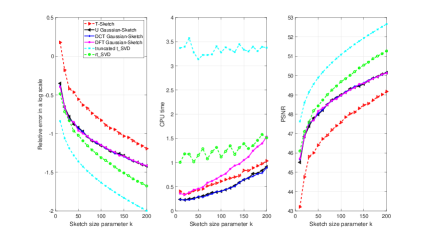
Figure 1: Performance comparison regarding the relative error (left), CPU time (middle), and PSNR (right). The data with PolyDecaySlow decaying spectrum is used here. Our method is the one based on the transformed domain.

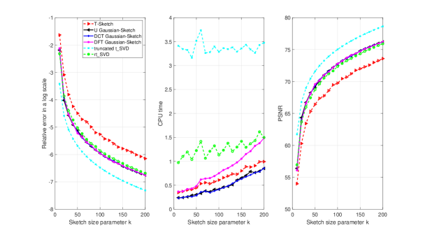
Figure 2: Performance comparison regarding the relative error (left), CPU time (middle), and PSNR (right). The data with PolyDecayMed decaying spectrum is used here. Our method is the one based on the transformed domain.

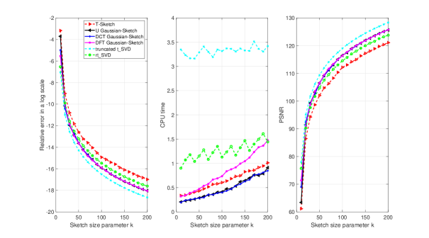
Figure 3: Performance comparison regarding the relative error (left), CPU time (middle), and PSNR (right). The data with PolyDecayFast decaying spectrum is used here. Our method is the one based on the transformed domain.

From Figures 1–3, we can see that the best one among two-sided Gaussian sketching algorithms based on the transformed domain (referred to the U Gaussian-Sketch, DCT Gaussian-Sketch, and DFT Gaussian-Sketch algorithms) is the DCT Gaussian-Sketch algorithm. Thus, two-sided Gaussian sketching algorithms based on the transformed domain chose the DCT transform to work best. In terms of CPU time, the DCT Gaussian-Sketch method is the fastest. In particular, as shown in Figures 2–3, the accuracy of the DCT Gaussian-Sketch method is better than the $rt$-SVD method and T-Sketch method for input tensor with PolyDecayMed decay spectrum and PolyDecayFast decay spectrum. In this case, with less storage and manipulation, the DCT Gaussian-Sketch method achieves better accuracy for the low-rank approximation. The DCT Gaussian-Sketch method is second only to the truncated $t$-SVD method in terms of accuracy but with faster speed.

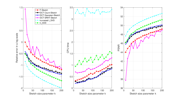
Figure 4: Performance comparison regarding the relative error (left), CPU time (middle), and PSNR (right). The data with PolyDecaySlow decaying spectrum is used here. Our method is the one based on the DCT transformed domain.

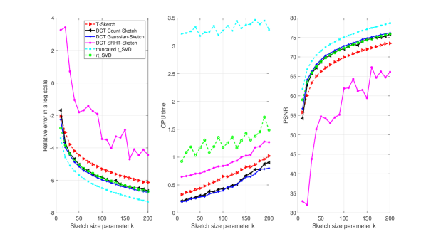
Figure 5: Performance comparison regarding the relative error (left), CPU time (middle), and PSNR (right). The data with PolyDecayMed decaying spectrum is used here. Our method is the one based on the DCT transformed domain.

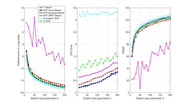
Figure 6: Performance comparison regarding the relative error (left), CPU time (middle), and PSNR (right). The data with PolyDecayFast decaying spectrum is used here. Our method is the one based on the DCT transformed domain.

From Figures 4–6, we see that the DCT Gaussian-Sketch algorithm has the best accuracy among the two-sided sketching algorithms based on the DCT transformed domain. The two-sided sketching algorithms based on the DCT transformed domain select the Gaussian tensor sketching operator with the best results. In terms of CPU time, the DCT Gaussian-Sketch method is the fastest. In particular, as shown in Figures 5–6, the accuracy of the DCT Gaussian-Sketch method is better than the $rt$-SVD method and T-Sketch method for input tensors with PolyDecayMed decay spectrum and PolyDecayFast decay spectrum. In this case, with less storage and manipulation, the DCT Gaussian-Sketch method achieves better accuracy for the low-rank approximation. The DCT Gaussian-Sketch method is second only to the truncated $t$-SVD method in terms of accuracy but is the fastest and far faster than the truncated $t$-SVD method.

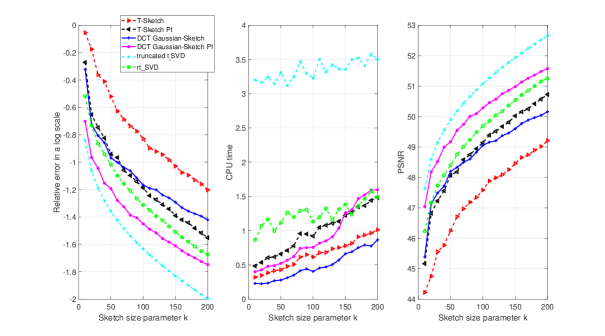
Figure 7: Performance comparison regarding the relative error (left), CPU time (middle), and PSNR (right). The data with PolyDecaySlow decaying spectrum is used here. Our method is the one based on the DCT transformed domain with power iteration.

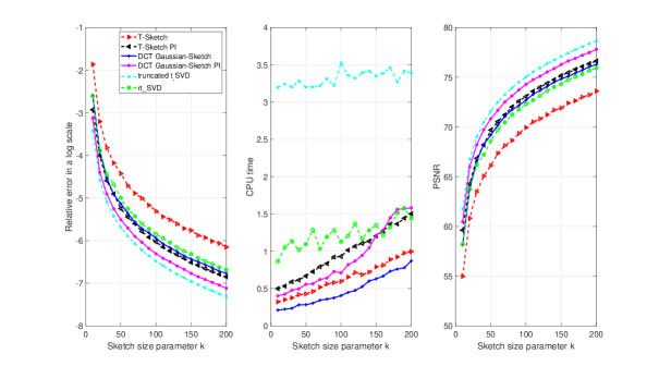
Figure 8: Performance comparison regarding the relative error (left), CPU time (middle), and PSNR (right). The data with PolyDecayMed decaying spectrum is used here. Our method is the one based on the DCT transformed domain with power iteration.

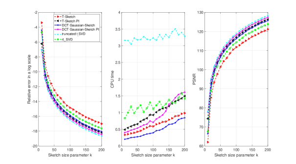
Figure 9: Performance comparison regarding the relative error (left), CPU time (middle), and PSNR (right). The data with PolyDecayFast decaying spectrum is used here. Our method is the one based on the DCT transformed domain with power iteration.

Figures 7–9 demonstrate the superiority of the proposed sketching algorithms, compared with the DCT Gaussian-Sketch method and $rt$-SVD method, the DCT Gaussian-Sketch PI ($q=1$) method achieves smaller relative error and higher PSNR. In terms of CPU time, the DCT Gaussian-Sketch method is the fastest. In particular, as shown in Figures 8–9, the accuracy of the DCT Gaussian-Sketch method is better than the $rt$-SVD method and T-Sketch method for input tensors with PolyDecayMed decay spectrum and PolyDecayFast decay spectrum. In this case, with less storage and manipulation, the DCT Gaussian-Sketch method achieves better accuracy for the low-rank approximation. The DCT Gaussian-Sketch PI ($q=1$) method is far superior to the T-Sketch PI ($q=1$) method in terms of time and accuracy. The DCT Gaussian-Sketch PI ($q=1$) method is second only to the truncated $t$-SVD method in terms of accuracy but is much faster in speed.

5.2 Real-world Data

We now conduct experiments on real-world data, i.e., color images and grayscale videos.

5.2.1 Color Images

Using DCT-Gaussian-Sketch-PI algorithm low-rank approximation, we compress three color images, i.e., HDU picture, with size of $1200\times 1800\times 3$, LONDON picture with size of $4775\times 7155\times 3$, and HDU 2D code with size of $800\times 800\times 3$. As shown in Figures 10, 13 and 16, tensor $\mathcal{A}$ has slow decaying spectrum ($q=0$), while it has faster decaying spectrum for $\mathcal{Z}=(\mathcal{A}\star{{}_{L}}\mathcal{A}^{\top})^{q}\star{{}_{L}}\mathcal{A}$ with $q=1$.

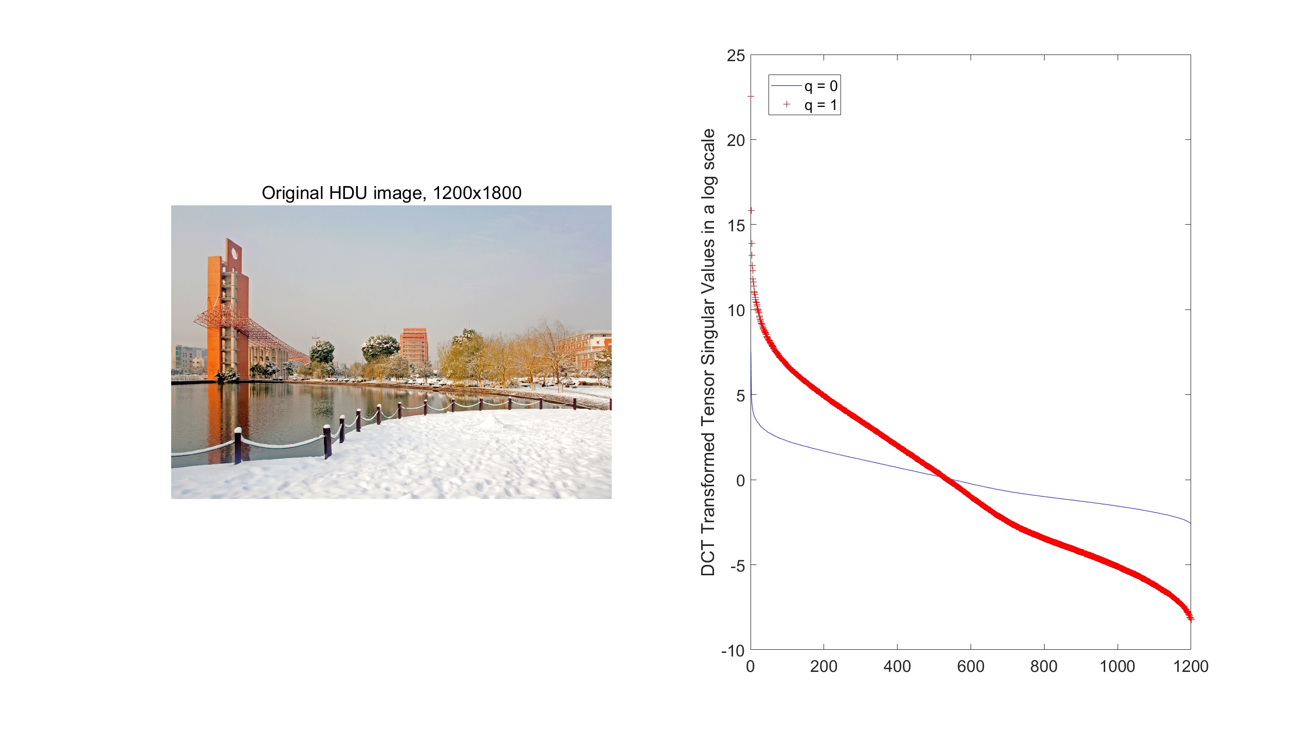
Figure 10: The original HDU image (left) and its Transformed tensor singular values with power iteration for $q=0$ and $q=1$ (right).

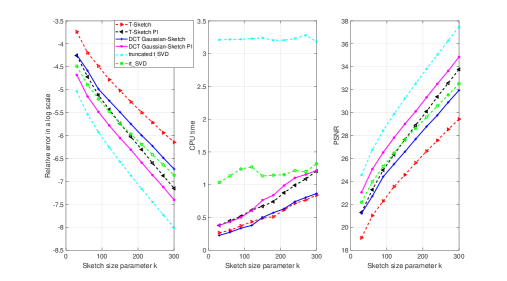
Figure 11: Performance comparison regarding the relative error (left), CPU time (middle), and PSNR (right). The data with HDU image is used here. Our method is the one based on the DCT transformed domain with power iteration.

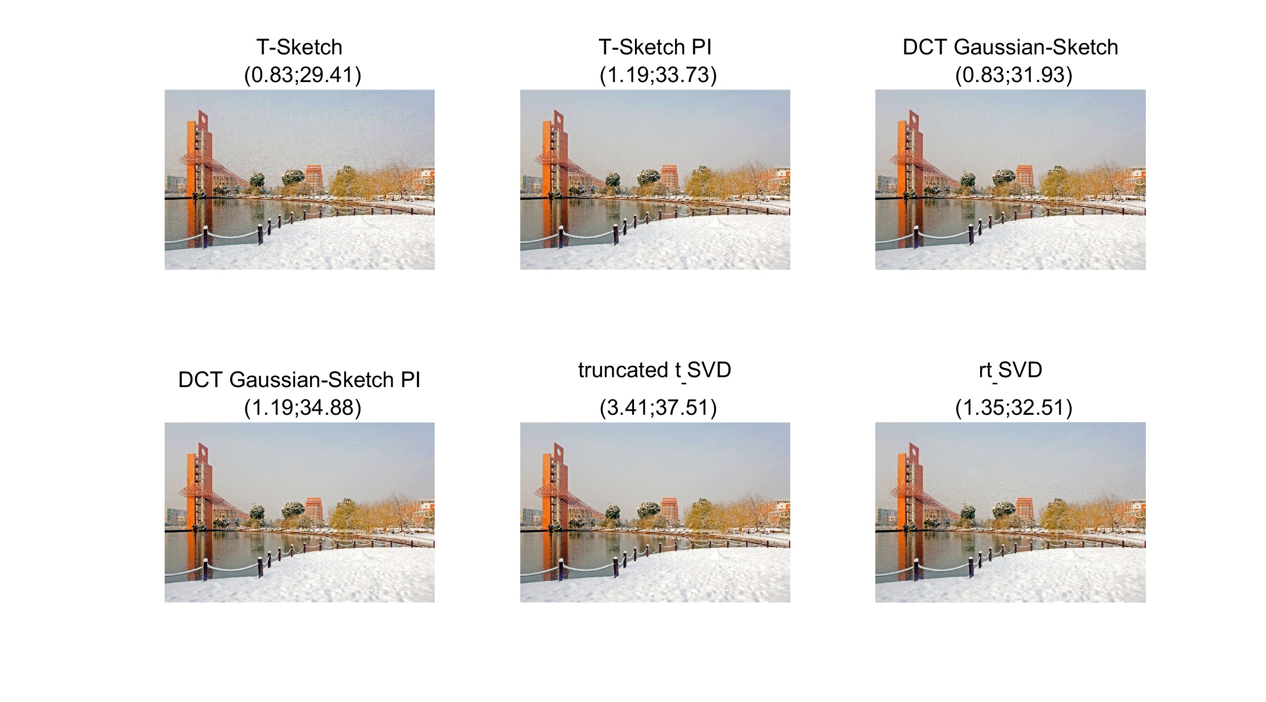
Figure 12: HDU image ($1200\times 1800\times 3$) experimental results, choosing sketch size $k$ = 300.

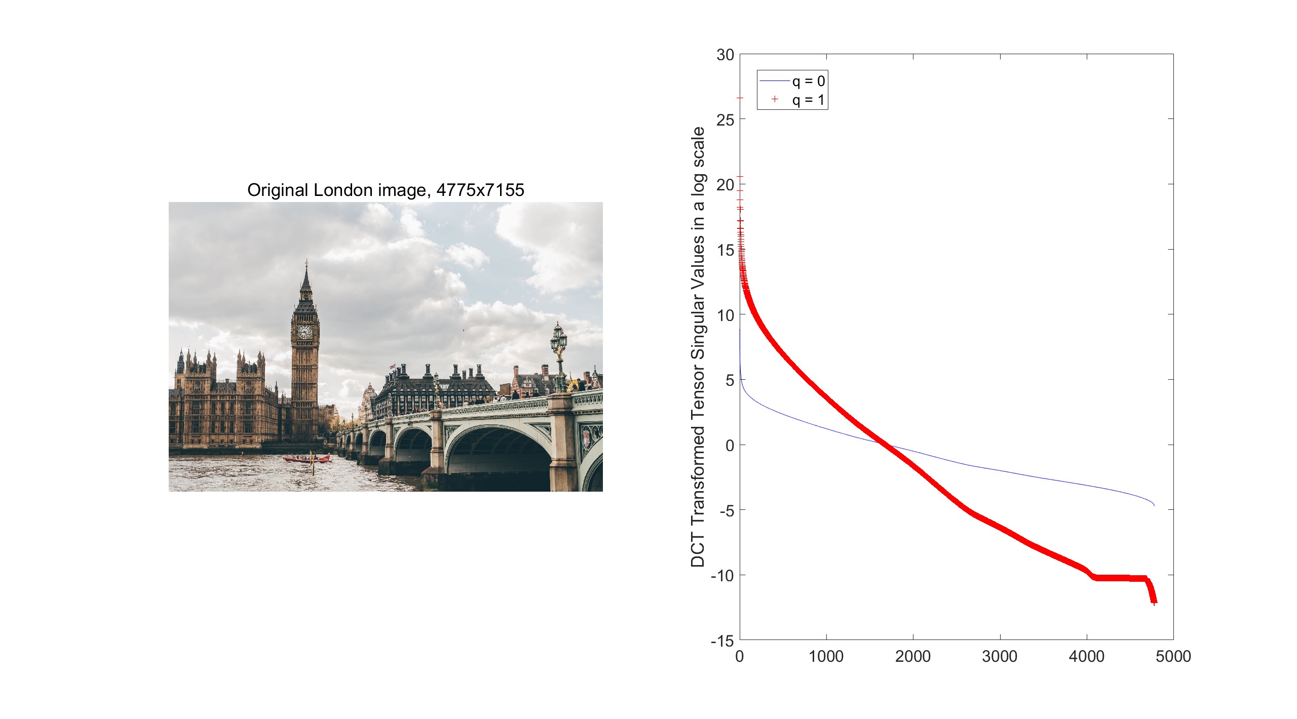
Figure 13: The original LONDON image and its Transformed Tensor Singular Values with power iteration for q=0 or q=1, respectively.

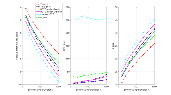
Figure 14: Performance comparison regarding the relative error (left), CPU time (middle), and PSNR (right). The data with LONDON image is used here. Our method is the one based on the DCT transformed domain with power iteration.

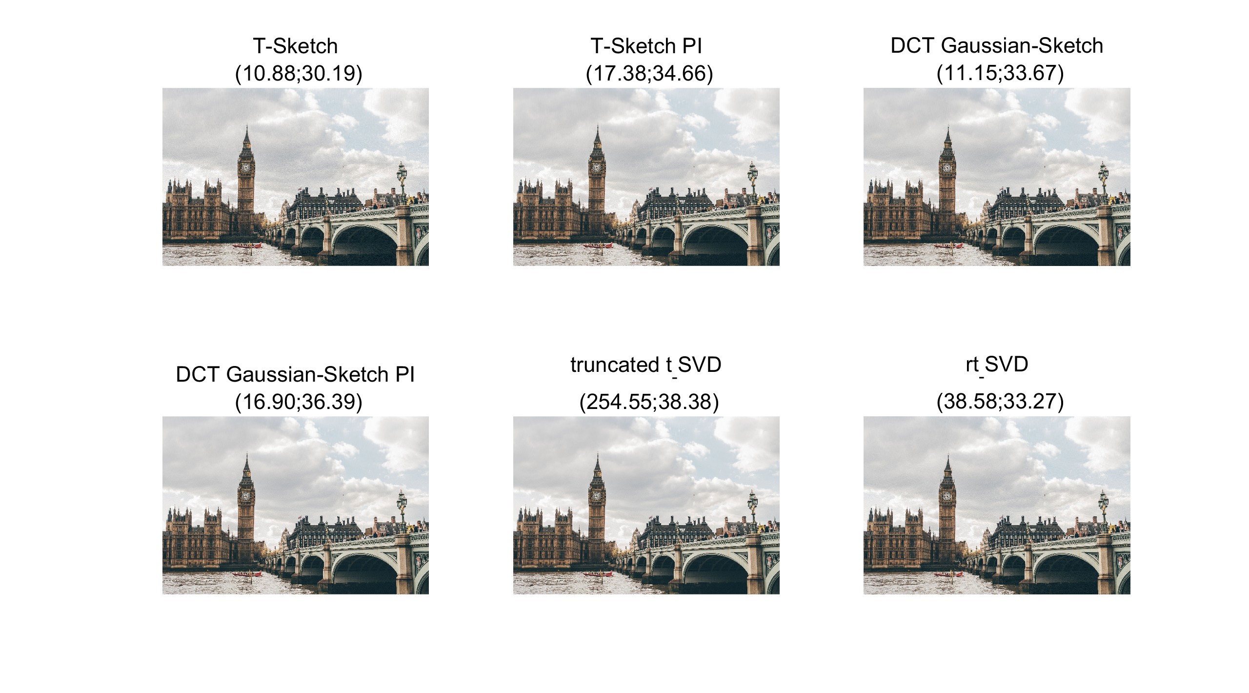
Figure 15: LONDON image ($4775\times 7155\times 3$) experimental results, choosing sketch size $k$ = 600.

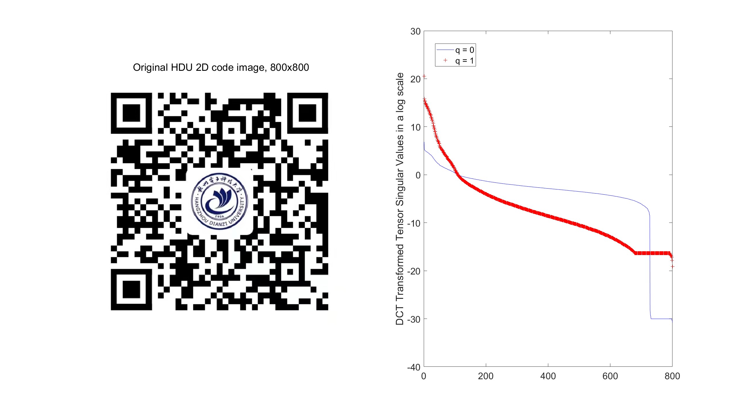
Figure 16: The original HDU 2D code image and its Transformed Tensor Singular Values with power iteration for q=0 or q=1, respectively.

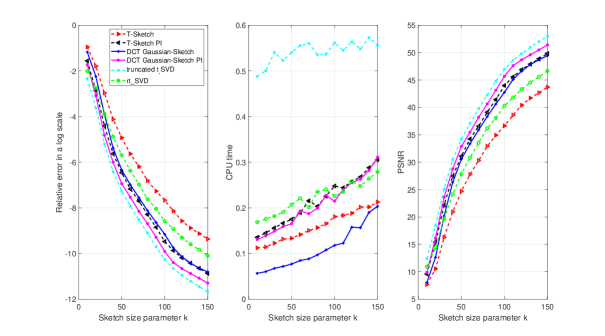
Figure 17: Performance comparison regarding the relative error (left), CPU time (middle), and PSNR (right). The data with HDU 2D code image is used here. Our method is the one based on the DCT transformed domain with power iteration.

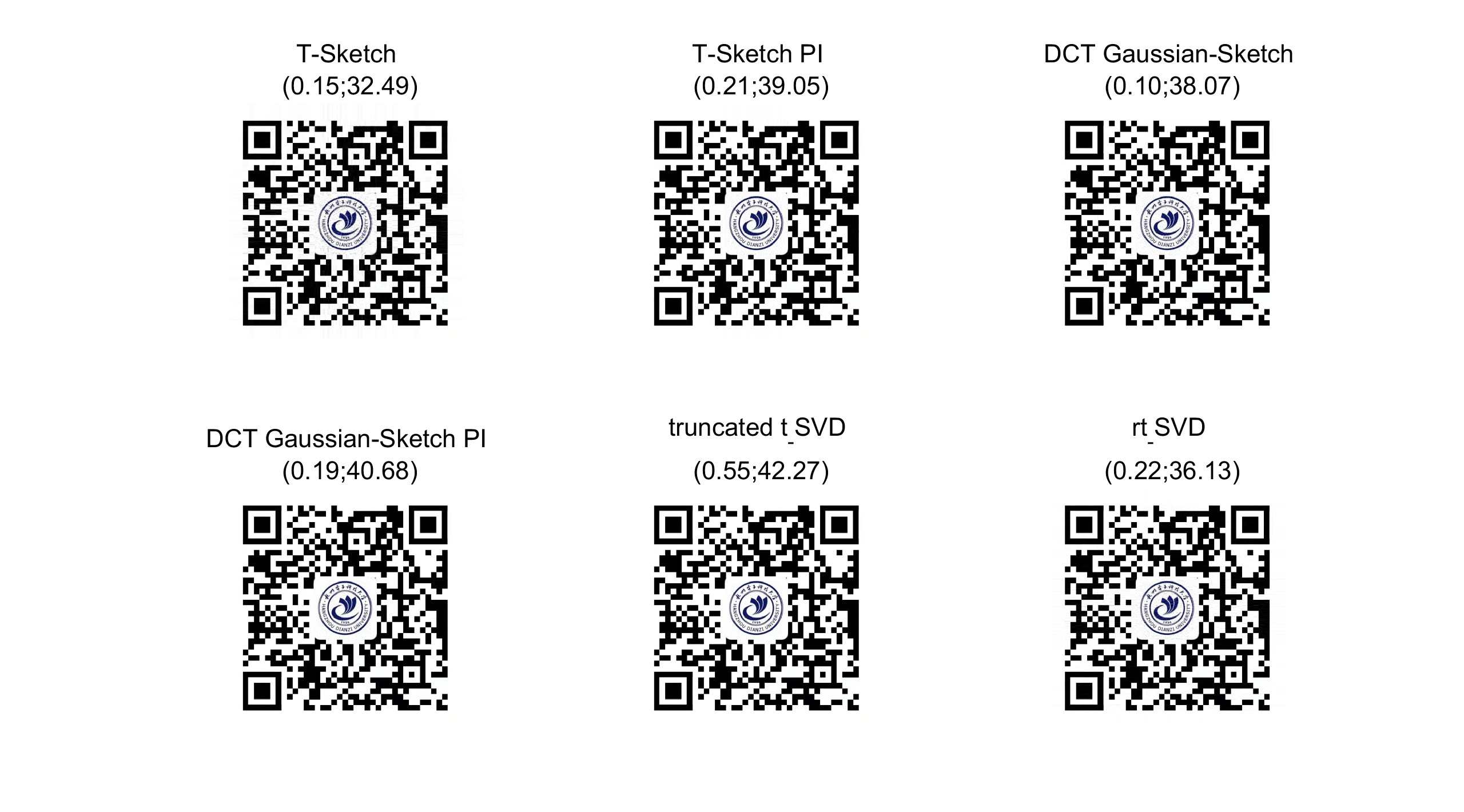
Figure 18: HDU 2D code ($800\times 800\times 3$) experimental results, choosing sketch size $k$=80.

From Figures 11–12, Figures 14–15 and Figures 17–18, we can see that DCT Gaussian-Sketch method achieves a better low-rank approximation as the sketch parameter size $k$ increases. In terms of CPU time, the DCT Gaussian-Sketch method is the fastest. In particular, as shown in Figures 14 and 17, the accuracy of the DCT Gaussian-Sketch method is better than the $rt$-SVD method and T-Sketch method. In this case, with less storage and manipulation, the DCT Gaussian-Sketch method achieves better accuracy for the low-rank approximation. The DCT Gaussian-Sketch PI ($q=1$) method is far superior to the T-Sketch PI ($q=1$) method in terms of CPU time and accuracy. The DCT Gaussian-Sketch PI ($q=1$) method is second only to the truncated $t\_$SVD method in terms of accuracy but is much faster in speed.

5.2.2 Grayscale Video

We finally evaluate the proposed sketching algorithms on the widely used YUV Video Sequences. Taking the ‘hall monitor’ video as an example and using the first 30 frames, a three order tensor with size of $144\times 176\times 30$ is then formed for this test. As shown in Figures 19–20, similar performance is obtained. In terms of CPU time, the DCT Gaussian-Sketch method is the fastest. The DCT Gaussian-Sketch PI ($q=1$) method is far superior to the T-Sketch PI ($q=1$) method in terms of CUP time and accuracy. Moreover, the DCT Gaussian-Sketch PI ($q=1$) method is second only to the truncated $t$-SVD method in terms of accuracy but is much faster in speed.

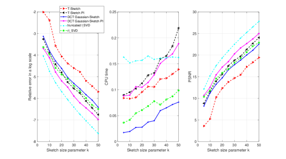
Figure 19: Performance comparison regarding the relative error (left), CPU time (middle), and PSNR (right). The data with grayscale video is used here. Our method is the one based on the DCT transformed domain with power iteration.($144\times 176\times 30$ tensor)

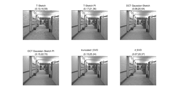
Figure 20: The first frame of the ‘hall monitor’ video ($144\times 176\times 30$) experimental results, choosing sketch size $k$ = 40.

6 Conclusion

In this paper, we introduced a low tubal rank tensor approximation model based on $\star_{L}$-product factorization. It is an extension of a new two-sided matrix sketching algorithm [38]. We proposed a novel two-sided sketching algorithm in the transformed domain, called L-TRP-SKETCH Algorithm. We also presented the DCT Gaussian-sketch PI algorithm, which can achieve more accurate approximate solutions. A rigorous theoretical analysis of the approximation error of the proposed DCT Gaussian-Sketch PI algorithm was also provided. Thorough experiments on low-rank approximation of synthetic data, color images and grayscale videos demonstrate the effectiveness and efficiency of the proposed algorithm in terms of computation time and low-rank approximation effects.

Appendix A

This subsection presents three matrix sketching techniques, i.e., Gaussian projection, subsampled randomized Hadamard transform (SRHT), and count sketch [50].

A.1. Gaussian Projection

The $n\times s$ Gaussian random projection matrix $S$ is a matrix formed by $S=G/\sqrt{s}$, where each entry of $G$ is sampled i.i.d. from $\mathcal{N}(0,1)$. For matrix $A\in\mathbb{R}^{m\times n}$, the time complexity of Gaussian projection is $\mathcal{O}(mns)$; see Algorithm 3 for the Gaussian projection process.

Algorithm 3 Gaussian Projection.

1:  Input: $A\in\mathbb{R}^{m\times n}$, parameter $s$

2:  function GaussianProjection($A,s$)

3:  Generate Gaussian random matrix $G$;

4:  $S=\frac{1}{\sqrt{s}}G$;

5:  $C=AS$;

6:  return $C\in\mathbb{R}^{m\times s}$.

A.2. Subsampled Randomized Hadamard Transform

The SRHT matrix is defined by $S=DH_{n}P/\sqrt{sn}$, where

• $D\in\mathbb{R}^{n\times n}$ is a diagonal matrix with diagonal entries sampled uniformly from $\{+1,1\}$.

• $H_{n}\in\mathbb{R}^{n\times n}$ is defined recursively by

  $$H_{n}=\begin{pmatrix}H_{\frac{n}{2}}&H_{\frac{n}{2}}\\ H_{\frac{n}{2}}&-H_{\frac{n}{2}}\end{pmatrix}\quad{\rm and}\quad H_{2}=\begin{pmatrix}+1&+1\\ +1&-1\end{pmatrix}.$$

  $\forall y\in\mathbb{R}^{n}$, the matrix vector product $y^{H}H_{n}$ can be performed in $\mathcal{O}({n\log n})$ by the fast Walsh-Hadamard transform algorithm in a divide-and-conquer fashion.

• $P\in\mathbb{R}^{n\times s}$ samples $s$ from the $n$ columns.

Algorithm 4 is not introduced in the main text here.

Algorithm 4 Subsampled Randomized Hadamard Transform (SRHT)

1:  Input: $A\in\mathbb{R}^{m\times n}$, parameter $s$.

2:  function SRHT($A,s$)

3:  $S=\frac{1}{\sqrt{sn}}DH_{n}P$;

4:  $C=AS$;

5:  return $C\in\mathbb{R}^{m\times s}$.

A.3. Count Sketch

There are two different ways to implement count sketch in “map-reduce fashion” and “streaming fashion”. These two approaches are equivalent, and thus we only discuss the streaming fashion below. The streaming fashion has two steps. Initially, the $m\times s$ matrix $C$ is set to all zero. Then, for each column of $A$, the sign is randomly flipped with a probability of 0.5 and added to a randomly selected column of $C$. This is outlined in Algorithm 5. The streaming fashion keeps the sketch $C$ in memory and scans the data $A$ in a single pass. If $A$ does not fit in memory, this approach is more efficient than the map-reduce fashion as it scans the columns in sequence. Additionally, if $A$ is a sparse matrix, randomly accessing the entries may not be efficient, and then it is better to access the columns sequentially.

Algorithm 5 Count Sketch in the Streaming Fashion.

1:  Input: $A\in\mathbb{R}^{m\times n}$, parameter $s$.

2:  function CountSketch($A,s$)

3:  Initialize $C$ to be an $m\times s$ all-zero matrix;

4:  for $i=1\;\textbf{to}\;n\ \textbf{do}$

5:   sample $l$ from the set $[s]$ uniformly at random;

6:   sample $g$ from the set $\{+1,-1\}$ uniformly at random;

7:   update the $l$-th column of $C$ by $c_{:l}\leftarrow c_{:l}+g_{a:i}$;

8:  end

9:  return $C\in\mathbb{R}^{m\times s}$.

It is noticed that the count sketch does not explicitly form the sketching matrix $S$. In fact, $S$ is such a matrix that each row has only one nonzero entry. The time complexity of Count sketch is $\mathcal{O}(\text{nnz(A)})$ (nnz(A) represent number of nonzeros of the matrix $A$).

Appendix B

In this section, taking the DCT Gaussian-Sketch algorithm as an example, we derive the error bound of the two-sided sketching algorithm.

A fact about random tensors are firstly given below.

Proposition 6.1

Assume $t>q+1$. Let $\mathcal{G}_{1}\in\mathbb{R}^{t\times q\times p}$ and $\mathcal{G}_{2}\in\mathbb{R}^{t\times l\times p}$ be Gaussian random tensors. For any tensor $\mathcal{B}$ with conforming dimensions,

$$\mathbb{E}{\parallel\mathcal{G}_{1}^{\dagger}\star{{}_{L}}\mathcal{G}_{2}\star{{}_{L}}\mathcal{B}\parallel}_{F}^{2}=\frac{q}{t-q-1}{\parallel\mathcal{B}\parallel}_{F}^{2}\ .$$

B.1. Results from Randomized Linear Algebra

Proposition 6.2

Fix $\mathcal{A}\in\mathbb{R}^{m\times n\times p}$ and let $\varrho<k$ be a natural number. Then the tensor $\mathcal{Q}\in\mathbb{R}^{m\times k\times p}$ calculated by Eq. (3.14) satisfies

$$\mathbb{E}_{\Omega}{\|\mathcal{A}-\mathcal{Q}\star{{}_{L}}\mathcal{Q}^{H}\star{{}_{L}}\mathcal{A}\|}_{F}^{2}\leq(1+f(\varrho,k)){\tau_{\varrho+1}}^{2}(\mathcal{A}\star{{}_{L}}\mathcal{A}^{H})\ .$$ (6.25)

An analogous result holds for the tensor $\mathcal{P}\in\mathbb{R}^{n\times k\times p}$ computed by Eq. (3.14), i.e.,

$$\mathbb{E}_{\Upsilon}{\|\mathcal{A}-\mathcal{A}\star{{}_{L}}\mathcal{P}\star{{}_{L}}\mathcal{P}^{H}\|}_{F}^{2}\leq(1+f(\varrho,k)){\tau_{\varrho+1}}^{2}(\mathcal{A}\star{{}_{L}}\mathcal{A}^{H})\ ,$$ (6.26)

where $f(\varrho,k)={\varrho}/({k-\varrho-1})$.

proof By Lemma 2.3 and the linearity of the expectation, we have

$$\mathbb{E}_{\Omega}\|\mathcal{A}-\mathcal{Q}_{L}\star{{}_{L}}\mathcal{Q}^{H}_{L}\star{{}_{L}}\mathcal{A}\|_{F}^{2} = {1\over p}\left(\sum_{i=1}^{p}\mathbb{E}\left\|\bar{\mathcal{A}}^{(i)}_{L}-\bar{\mathcal{Q}}^{(i)}_{L}\left(\bar{\mathcal{Q}}^{(i)}_{L}\right)^{H}\bar{\mathcal{A}}^{(i)}_{L}\right\|_{F}^{2}\right).$$

By [51, Theorem 10.5], we have

$$\mathbb{E}{\|{\bar{\mathcal{A}}}^{(i)}_{\text{$F_{n_{3}}$}}-\bar{\mathcal{Q}}^{(i)}_{\text{$F_{n_{3}}$}}(\bar{\mathcal{Q}}^{(i)}_{\text{$F_{n_{3}}$}})^{H}{\bar{\mathcal{A}}}^{(i)}_{\text{$F_{n_{3}}$}}\|}_{F}^{2}\leq(1+f(\varrho,k))\cdot\tau_{\varrho+1}^{2}(\bar{\mathcal{A}}^{(i)}_{\text{$F_{n_{3}}$}}(\bar{\mathcal{A}}^{(i)}_{\text{$F_{n_{3}}$}})^{H})\ .$$

Similarly, we know from [41] that multiplying by a unitary matrix will not change the Frobenius norm, i.e., the Frobenius norm keeps the unitary matrix unchanged. Thus we have

$$\mathbb{E}{\|{\bar{\mathcal{A}}}^{(i)}_{L}-\bar{\mathcal{Q}}^{(i)}_{L}(\bar{\mathcal{Q}}^{(i)}_{L})^{H}{\bar{\mathcal{A}}}^{(i)}_{L}\|}_{F}^{2}\leq(1+f(\varrho,k))\cdot\tau_{\varrho+1}^{2}(\bar{\mathcal{A}}^{(i)}_{L}(\bar{\mathcal{A}}^{(i)}_{L})^{H})$$

and

$$\mathbb{E}_{\Omega}\|\mathcal{A}-\mathcal{Q}_{L}\star{{}_{L}}\mathcal{Q}^{H}_{L}\star{{}_{L}}\mathcal{A}\|_{F}^{2} \leq\frac{1}{p}(1+f(\varrho,k))\cdot(\sum_{i=1}^{p}\tau_{\varrho+1}^{2}(\bar{\mathcal{A}}^{(i)}_{L}(\bar{\mathcal{A}}^{(i)}_{L})^{H}))$$

$$=(1+f(\varrho,k))\cdot\tau_{\varrho+1}^{2}(\mathcal{A}\star{{}_{L}}\mathcal{A}^{H})\ .$$

Similarly, there is

$$\mathbb{E}_{\Upsilon}{\|\mathcal{A}-\mathcal{A}\star{{}_{L}}\mathcal{P}\star{{}_{L}}\mathcal{P}^{H}\|}_{F}^{2}\leq(1+\frac{\varrho}{k-\varrho-1}){\tau_{\varrho+1}}^{2}(\mathcal{A}\star{{}_{L}}\mathcal{A}^{H})\ ,$$ (6.27)

which completes the proof.

Let $\hat{\mathcal{A}}$ be the transformed tensor tubal rank $k$ approximation of $\mathcal{A}$ obtained by the DCT Gaussian-sketch algorithm. We now split the error ${\|\mathcal{A}-\hat{\mathcal{A}}\|}_{F}^{2}$ into two parts by the proposition below.

Proposition 6.3

Let $\hat{\mathcal{A}}$ be the transformed tensor tubal rank $k$ approximation of $\mathcal{A}\in\mathbb{R}^{m\times n\times p}$ obtained by the DCT Gaussian-sketch algorithm, with $\mathcal{Q}$, $\mathcal{C}$ and $\mathcal{P}$ being the intermediate tensors obtained by the DCT Gaussian-Sketch algorithm satisfying $\mathcal{Q}^{H}\star{{}_{L}}\mathcal{Q}=\mathcal{I}_{kkp}$,$\mathcal{P}\star{{}_{L}}\mathcal{P}^{H}=\mathcal{I}_{nnp}$. Then

$${\|\mathcal{A}-\hat{\mathcal{A}}\|}_{F}^{2}={\|\mathcal{A}-\mathcal{Q}\star{{}_{L}}\mathcal{Q}^{H}\star{{}_{L}}\mathcal{A}\star{{}_{L}}\mathcal{P}\star{{}_{L}}\mathcal{P}^{H}\|}_{F}^{2}+{\|\mathcal{C}-\mathcal{Q}^{H}\star{{}_{L}}\mathcal{A}\star{{}_{L}}\mathcal{P}\|}_{F}^{2}\ .$$ (6.28)

proof Since $\hat{\mathcal{A}}=\mathcal{Q}\star{{}_{L}}\mathcal{C}\star{{}_{L}}\mathcal{P}^{H}$, we have

$$\|\mathcal{A}-\hat{\mathcal{A}}\|_{F}^{2}$$

$$= \frac{1}{p}\sum_{i=1}^{p}{\|\bar{\mathcal{A}}_{{\Phi}}-\bar{\hat{\mathcal{A}}}_{{\Phi}}\|}_{F}^{2}$$

$$= \frac{1}{p}\sum_{i=1}^{p}({\|\bar{\mathcal{A}}_{{\Phi}}-\bar{\mathcal{Q}}_{{\Phi}}\bar{\mathcal{Q}}^{H}_{{\Phi}}\bar{{\mathcal{A}}}_{{\Phi}}\bar{\mathcal{P}}_{{\Phi}}\bar{\mathcal{P}}^{H}\|}_{F}^{2}+{\|\bar{\mathcal{C}}_{{\Phi}}-\bar{\mathcal{Q}}^{H}_{{\Phi}}\bar{{\mathcal{A}}}_{{\Phi}}\bar{\mathcal{P}}_{{\Phi}}\|}_{F}^{2})$$

$$= {\|\mathcal{A}-\mathcal{Q}\star{{}_{L}}\mathcal{Q}^{H}\star{{}_{L}}\mathcal{A}\star{{}_{L}}\mathcal{P}\star{{}_{L}}\mathcal{P}^{H}\|}_{F}^{2}+{\|\mathcal{C}-\mathcal{Q}^{H}\star{{}_{L}}\mathcal{A}\star{{}_{L}}\mathcal{P}\|}_{F}^{2}\ .$$

The first and last equations are known by Lemma 2.3, and the second equation is known by [38, A.6] Appendix A.

Theorem 6.4

For any natural number $\varrho<k-1$, it holds that

$$\mathbb{E}_{\Upsilon}\mathbb{E}_{\Omega}{\|\mathcal{A}-\mathcal{Q}\star{{}_{L}}\mathcal{Q}^{H}\star{{}_{L}}\mathcal{A}\star{{}_{L}}\mathcal{P}\star{{}_{L}}\mathcal{P}^{H}\|}_{F}^{2}\leq{(1+\frac{2\varrho}{k-\varrho-1})}\tau_{\varrho+1}^{2}(\mathcal{A}\star{{}_{L}}\mathcal{A}^{H})\ .$$ (6.29)

proof We have

$$\mathbb{E}_{\Upsilon}\mathbb{E}_{\Omega}{\|\mathcal{A}-\mathcal{Q}\star{{}_{L}}\mathcal{Q}^{H}\star{{}_{L}}\mathcal{A}\star{{}_{L}}\mathcal{P}\star{{}_{L}}\mathcal{P}^{H}\|}_{F}^{2}$$

$$= \frac{1}{p}\sum_{i=1}^{p}\mathbb{E}_{\Upsilon}\mathbb{E}_{\Omega}{\|\bar{\mathcal{A}}_{{\Phi}}-\bar{\mathcal{Q}}_{{\Phi}}\bar{\mathcal{Q}}^{H}_{{\Phi}}\bar{{\mathcal{A}}}_{{\Phi}}\bar{\mathcal{P}}_{{\Phi}}\bar{\mathcal{P}}^{H}\|}_{F}^{2}$$

$$\leq {(1+\frac{2\varrho}{k-\varrho-1})}\tau_{\varrho+1}^{2}(\mathcal{A}\star{{}_{L}}\mathcal{A}^{H})\ .$$

The first equation is known by Lemma 2.3, and the inequality is known by [38, A.5] Appendix A.

B.2. Decomposition of the Core Tensor Approximation Error

The first step in the argument is to obtain a formula for the error in the approximation $(\mathcal{C}-\mathcal{Q}^{H}\star{{}_{L}}\mathcal{A}\star{{}_{L}}\mathcal{P})$. The core tensor $\mathcal{C}\in\mathbb{R}^{k\times k\times p}$ is defined in Eq. (3.17), and the orthonormal tensors $\mathcal{P}\in\mathbb{R}^{n\times k\times p}$ and $\mathcal{Q}\in\mathbb{R}^{m\times k\times p}$ are constructed in Eq. (3.14). Let us introduce tensors whose ranges are complementary to those of $\mathcal{P}$ and $\mathcal{Q}$, i.e.,

$$\mathcal{P}_{\perp}\star{{}_{L}}\mathcal{P}_{\perp}^{H} =\mathcal{I}_{mmp}-\mathcal{P}\star{{}_{L}}\mathcal{P}^{H},\mathcal{P}_{\perp}\in\mathbb{R}^{n\times(n-k)\times p},$$ (6.30)

$$\mathcal{Q}_{\perp}\star{{}_{L}}\mathcal{Q}_{\perp}^{H} =\mathcal{I}_{mmp}-\mathcal{Q}\star{{}_{L}}\mathcal{Q}^{H},\mathcal{Q}_{\perp}\in\mathbb{R}^{m\times(m-k)\times p}.$$ (6.31)

The columns of $\mathcal{P}_{\perp}$ and $\mathcal{Q}_{\perp}$ are orthonormal, separately. Next, we introduce the subtensors, i.e.,

$$\begin{split}\Phi_{1}:={\Phi}\star{{}_{L}}\mathcal{Q}\in\mathbb{R}^{s\times k\times p},\ {\Phi}_{2}:=\Phi\star{{}_{L}}\mathcal{Q}_{\perp}\in\mathbb{R}^{s\times(m-k)\times p},\\ {\Psi}_{1}^{H}:=\mathcal{P}^{H}\star{{}_{L}}{\Psi}^{H}\in\mathbb{R}^{k\times s\times p},\ {\Psi}_{2}^{H}:={\mathcal{P}^{H}_{\perp}}\star{{}_{L}}{\displaystyle\Psi^{H}}\in\mathbb{R}^{(n-k)\times s\times p}.\end{split}$$ (6.32)

With these notations at hand, we can state and prove the lemma below.

Lemma 6.5

(Decomposition of the Core Tensor Approximation) Assume the tensor transformed tubal rank of $\Phi_{1}$ and ${\Psi}_{1}$ is $k$ and $s$, respectively. Then

$$\ \mathcal{C}-\mathcal{Q}^{H}\star{{}_{L}}\mathcal{A}\star{{}_{L}}\mathcal{P}$$

$$= \ \Phi_{1}^{\dagger}\star{{}_{L}}\Phi_{2}\star{{}_{L}}(\mathcal{Q}^{H}_{\perp}\star{{}_{L}}\mathcal{A}\star{{}_{L}}\mathcal{P})+(\mathcal{Q}^{H}\star{{}_{L}}\mathcal{A}\star{{}_{L}}\mathcal{P}_{\perp})\star{{}_{L}}\Psi_{2}^{\dagger}\star{{}_{L}}(\Psi^{\dagger}_{1})^{H}$$

$$+\Phi_{1}^{\dagger}\star{{}_{L}}\Phi_{2}\star{{}_{L}}(\mathcal{Q}^{H}_{\perp}\star{{}_{L}}\mathcal{A}\star{{}_{L}}\mathcal{P}_{\perp})\star{{}_{L}}\Psi_{2}^{\dagger}\star{{}_{L}}(\Psi^{\dagger}_{1})^{H}.$$

proof Adding and subtracting terms, we write the core sketch $\mathcal{Z}$ as

$$\mathcal{Z}= \ \Phi\star{{}_{L}}\mathcal{A}\star{{}_{L}}{\Psi}^{H}$$

$$= \ \Phi\star{{}_{L}}(\mathcal{A}-\mathcal{Q}\star{{}_{L}}\mathcal{Q}^{H}\star{{}_{L}}\mathcal{A}\star{{}_{L}}\mathcal{P}\star{{}_{L}}\mathcal{P}^{H})\star{{}_{L}}{\Psi}^{H}$$

$$+(\Phi\star{{}_{L}}\mathcal{Q})\star{{}_{L}}(\mathcal{Q}^{H}\star{{}_{L}}\mathcal{A}\star{{}_{L}}\mathcal{P})\star{{}_{L}}(\mathcal{P}^{H}\star{{}_{L}}\Psi^{H}).$$

Using Eq. (6.32), we identify the tensors $\Phi_{1}$ and ${\Psi}_{1}$. After left-multiplying by $\Phi^{\dagger}_{1}$ and right-multiplying by $({\Psi^{\dagger}_{1}})^{H}$, we have

$$\mathcal{C} =\ {\Phi}^{\dagger}_{1}\star{{}_{L}}\mathcal{Z}\star{{}_{L}}({\Psi^{\dagger}_{1}})^{H}$$

$$=\ {\Phi}^{\dagger}_{1}\star{{}_{L}}\Phi\star{{}_{L}}(\mathcal{A}-\mathcal{Q}\star{{}_{L}}\mathcal{Q}^{H}\star{{}_{L}}\mathcal{A}\star{{}_{L}}\mathcal{P}\star{{}_{L}}\mathcal{P}^{H})\star{{}_{L}}\Psi^{H}\star{{}_{L}}({\Psi^{\dagger}_{1}})^{H}$$

$$\quad\ \ +\mathcal{Q}^{H}\star{{}_{L}}\mathcal{A}\star{{}_{L}}\mathcal{P}.$$

We have identified the core tensor $\mathcal{C}$ defined in (3.17). Moving the term $\mathcal{Q}^{H}\star{{}_{L}}\mathcal{A}\star{{}_{L}}\mathcal{P}$ to the left-hand side to isolate the approximation error, we have

$${\Phi}^{\dagger}_{1}\star{{}_{L}}\Phi ={\Phi}^{\dagger}_{1}\star{{}_{L}}\Phi\star{{}_{L}}\mathcal{Q}\star{{}_{L}}\mathcal{Q}^{H}+{\Phi}^{\dagger}_{1}\star{{}_{L}}\Phi\star{{}_{L}}\mathcal{Q}_{\perp}\star{{}_{L}}\mathcal{Q}^{H}_{\perp}$$

$$=\mathcal{Q}^{H}+{\Phi}^{\dagger}_{1}\star{{}_{L}}\Phi_{2}\star{{}_{L}}\mathcal{Q}^{H}_{\perp}\ .$$

Likewise,

$$\ {\Psi}^{H}\star{{}_{L}}({\Psi}^{\dagger}_{1})^{H}$$

$$= \ \mathcal{P}\star{{}_{L}}\mathcal{P}^{H}\star{{}_{L}}{\Psi}^{H}\star{{}_{L}}({\Psi}^{\dagger}_{1})^{H}+\mathcal{P}_{\perp}\star{{}_{L}}\mathcal{P}_{\perp}^{H}\star{{}_{L}}{\Psi}^{H}\star{{}_{L}}({\Psi}^{\dagger}_{1})^{H}$$

$$= \ \mathcal{P}+\mathcal{P}_{\perp}\star{{}_{L}}{{\Psi}_{2}^{H}}\star{{}_{L}}({\Psi}^{\dagger}_{1})^{H}.$$

Combining the last three displays, we have

$$\ \mathcal{C}-\mathcal{Q}^{H}\star{{}_{L}}\mathcal{A}\star{{}_{L}}\mathcal{P}$$

$$= \ (\mathcal{Q}^{H}+{\Phi}^{\dagger}_{1}\star{{}_{L}}\Phi_{2}\star{{}_{L}}\mathcal{Q}_{\perp}^{H})\star{{}_{L}}(\mathcal{A}-\mathcal{Q}\star{{}_{L}}\mathcal{Q}^{H}\star{{}_{L}}\mathcal{A}\star{{}_{L}}\mathcal{P}\star{{}_{L}}\mathcal{P}^{H})\star{{}_{L}}(\mathcal{P}$$

$$+\mathcal{P}_{\perp}\star{{}_{L}}{{\Psi}_{2}^{H}}\star{{}_{L}}({\Psi}^{\dagger}_{1})^{H}).$$

Expanding the expression and using the orthogonality relations $\mathcal{Q}^{H}\star{{}_{L}}\mathcal{Q}=\mathcal{I}_{kkp}$, $\mathcal{Q}_{\perp}^{H}\star{{}_{L}}\mathcal{Q}=\mathcal{O}$, $\mathcal{P}^{H}\star{{}_{L}}\mathcal{P}=\mathcal{I}_{kkp}$, and $\mathcal{P}_{\perp}^{H}\star{{}_{L}}\mathcal{P}=\mathcal{O}$, we complete the proof.

B.3. Probabilistic Analysis of the Core Tensor

We can then study the probabilistic behavior of the error $(\mathcal{C}-\mathcal{Q}^{H}\star{{}_{L}}\mathcal{A}\star{{}_{L}}\mathcal{P})$, conditional on $\mathcal{Q}$ and $\mathcal{P}$.

Lemma 6.6

(Probabilistic Analysis of the Core Tensor) Assume that the dimension reduction tensors $\Phi$ and $\Psi$ are Gaussian linear sketching operators. When $s\geq k$, it holds that

$$\mathbb{E}_{\Phi,\Psi}[\mathcal{C}-\mathcal{Q}^{H}\star{{}_{L}}\mathcal{A}\star{{}_{L}}\mathcal{P}]=\mathcal{O}.$$ (6.33)

When $s>k+1$, the error can be expressed as

$$\ \mathbb{E}_{\Phi,\Psi}{\|\mathcal{C}-\mathcal{Q}^{T}\star{{}_{L}}\mathcal{A}\star{{}_{L}}\mathcal{P}\|}_{F}^{2}$$

$$= \ \frac{k}{s-k-1}{\|\mathcal{A}-\mathcal{Q}\star{{}_{L}}\mathcal{Q}^{H}\star{{}_{L}}\mathcal{A}\star{{}_{L}}\mathcal{P}\star{{}_{L}}\mathcal{P}^{H}\|}_{F}^{2}$$

$$\ +\frac{k(2k+1-s)}{(s-k-1)^{2}}{\|\mathcal{Q}_{\perp}^{H}\star{{}_{L}}\mathcal{A}\star{{}_{L}}\mathcal{P}_{\perp}\|}_{F}^{2}\ .$$

In particular, when $s<2k+1$, the last term is nonnegative; and when $s\geq 2k+1$, the last term is nonpositive.

proof Since $\Phi$ is a Gaussian linear sketching operator, the orthogonal subtensors $\Phi_{1}$ and $\Phi_{2}$ are also Gaussian linear sketching operators because of the marginal property of the normal distribution. Likewise, $\Psi_{1}$ and $\Psi_{2}$ are Gaussian linear sketching operators. Provided that $s\geq k$, the tensor transformed tubal rank of $\Phi_{1}$ and $\Psi_{1}$ is $k$. Thus,

$$\ \mathbb{E}_{\Phi,\Psi}[\mathcal{C}-\mathcal{Q}^{H}\star{{}_{L}}\mathcal{A}\star{{}_{L}}\mathcal{P}]$$

$$= \ \mathbb{E}_{\Phi_{1}}\mathbb{E}_{\Phi_{2}}[\Phi_{1}^{\dagger}\star{{}_{L}}\Phi_{2}\star{{}_{L}}(\mathcal{Q}_{\perp}^{H}\star{{}_{L}}\mathcal{A}\star{{}_{L}}\mathcal{P})]$$

$$\ +\mathbb{E}_{\Psi_{1}}\mathbb{E}_{\Psi_{2}}[(\mathcal{Q}^{H}\star{{}_{L}}\mathcal{A}\star{{}_{L}}\mathcal{P}_{\perp})\star{{}_{L}}\Psi_{2}^{H}\star{{}_{L}}(\Psi_{1}^{\dagger})^{H}]$$

$$\ +\mathbb{E}[\Phi_{1}^{\dagger}\star{{}_{L}}\Phi_{2}\star{{}_{L}}(\mathcal{Q}_{\perp}^{H}\star{{}_{L}}\mathcal{A}\star{{}_{L}}\mathcal{P}_{\perp})\star{{}_{L}}\Psi_{2}^{H}\star{{}_{L}}(\Psi_{1}^{\dagger})^{H}]\ .$$

We have used the decomposition of the approximation error from Lemma 6.5. Then we invoke independence to write the expectations as iterated expectations. Since $\Phi_{2}$ and $\Psi_{2}$ have to mean zero. This formula makes it clear that the approximation error has to mean zero.

To study the fluctuations, applying the independence and zero-mean property of $\Phi_{2}$ and $\Psi_{2}$, we have

$$\ \mathbb{E}_{\Phi,\Psi}{\|\mathcal{C}-\mathcal{Q}^{H}\star{{}_{L}}\mathcal{A}\star{{}_{L}}\mathcal{P}\|}_{F}^{2}$$

$$= \ \mathbb{E}_{\Phi}{\|\Phi_{1}^{\dagger}\star{{}_{L}}\Phi_{2}\star{{}_{L}}(\mathcal{Q}_{\perp}^{H}\star{{}_{L}}\mathcal{A}\star{{}_{L}}\mathcal{P})\|}_{F}^{2}$$

$$\ +\mathbb{E}_{\Psi}{\|(\mathcal{Q}^{H}\star{{}_{L}}\mathcal{A}\star{{}_{L}}\mathcal{P}_{\perp})\star{{}_{L}}\Psi_{2}^{H}\star{{}_{L}}(\Psi_{1}^{\dagger})^{H}\|}_{F}^{2}$$

$$\ +\mathbb{E}_{\Phi}\mathbb{E}_{\Psi}{\|\Phi_{1}^{\dagger}\star{{}_{L}}\Phi_{2}\star{{}_{L}}(\mathcal{Q}_{\perp}^{H}\star{{}_{L}}\mathcal{A}\star{{}_{L}}\mathcal{P}_{\perp})\star{{}_{L}}\Psi_{2}^{H}\star{{}_{L}}(\Psi_{1}^{\dagger})^{H}\|}_{F}^{2}.$$

Invoking Proposition 6.1 yields

$$\ \mathbb{E}_{\Phi,\Psi}{\|\mathcal{C}-\mathcal{Q}^{H}\star{{}_{L}}\mathcal{A}\star{{}_{L}}\mathcal{P}\|}_{F}^{2}$$

$$= \ \frac{k}{s-k-1}[{\|\mathcal{Q}_{\perp}^{H}\star{{}_{L}}\mathcal{A}\star{{}_{L}}\mathcal{P}\|}_{F}^{2}+{\|\mathcal{Q}^{H}\star{{}_{L}}\mathcal{A}\star{{}_{L}}\mathcal{P}_{\perp}\|}_{F}^{2}$$

$$\ +\frac{k}{s-k-1}{\|\mathcal{Q}_{\perp}^{H}\star{{}_{L}}\mathcal{A}\star{{}_{L}}\mathcal{P}_{\perp}\|}_{F}^{2}]$$

$$= \ \frac{k}{s-k-1}[{\|\mathcal{Q}_{\perp}^{H}\star{{}_{L}}\mathcal{A}\star{{}_{L}}\mathcal{P}\|}_{F}^{2}+{\|\mathcal{Q}^{H}\star{{}_{L}}\mathcal{A}\star{{}_{L}}\mathcal{P}_{\perp}\|}_{F}^{2}+{\|\mathcal{Q}_{\perp}^{H}\star{{}_{L}}\mathcal{A}\star{{}_{L}}\mathcal{P}_{\perp}\|}_{F}^{2}$$

$$\ +\frac{2k+1-s}{s-k-1}{\|\mathcal{Q}_{\perp}^{H}\star{{}_{L}}\mathcal{A}\star{{}_{L}}\mathcal{P}_{\perp}\|}_{F}^{2}]\ .$$

Using the Pythagorean Theorem to combine the terms on the above equation, we have

$$\ \mathbb{E}_{\Phi,\Psi}{\|\mathcal{C}-\mathcal{Q}^{H}\star{{}_{L}}\mathcal{A}\star{{}_{L}}\mathcal{P}\|}_{F}^{2}$$

$$= \ \frac{k}{s-k-1}{\|\mathcal{A}-\mathcal{Q}\star{{}_{L}}\mathcal{Q}^{H}\star{{}_{L}}\mathcal{A}\star{{}_{L}}\mathcal{P}\star{{}_{L}}\mathcal{P}^{H}\|}_{F}^{2}$$

$$\ +\frac{k(2k+1-s)}{(s-k-1)^{2}}{\|\mathcal{Q}_{\perp}^{H}\star{{}_{L}}\mathcal{A}\star{{}_{L}}\mathcal{P}_{\perp}\|}_{F}^{2}\ .$$

This completes the proof.

References

- [1] T.-X. Jiang, T.-Z. Huang, X.-L. Zhao, L.-J. Deng, and Y. Wang, “A novel tensor-based video rain streaks removal approach via utilizing discriminatively intrinsic priors,” in Proceedings of the 2017 IEEE Conference on Computer Vision and Pattern Recognition. IEEE, 2017, pp. 4057–4066.
- [2] T.-K. Kim, S.-F. Wong, and R. Cipolla, “Tensor canonical correlation analysis for action classification,” in Proceedings of the 2007 IEEE Conference on Computer Vision and Pattern Recognition. IEEE, 2007, pp. 1–8.
- [3] B. Du, M. Zhang, L. Zhang, R. Hu, and D. Tao, “Pltd: Patch-based low-rank tensor decomposition for hyperspectral images,” IEEE Transactions on Multimedia, vol. 19, no. 1, pp. 67–79, 2016.
- [4] N. Renard, S. Bourennane, and J. Blanc-Talon, “Denoising and dimensionality reduction using multilinear tools for hyperspectral images,” IEEE Geoscience and Remote Sensing Letters, vol. 5, no. 2, pp. 138–142, 2008.
- [5] Wu W H, Huang T Z, Zhao X L, et al. Hyperspectral Image Denoising via Tensor Low-Rank Prior and Unsupervised Deep Spatial–Spectral Prior[J]. IEEE Transactions on Geoscience and Remote Sensing, 2022, 60: 1-14.
- [6] Wang J L, Huang T Z, Zhao X L, et al. CoNoT: Coupled Nonlinear Transform-Based Low-Rank Tensor Representation for Multidimensional Image Completion[J]. IEEE Transactions on Neural Networks and Learning Systems, 2022.
- [7] L. De Lathauwer, “Signal processing based on multilinear algebra,” Ph.D. dissertation, Katholieke Universiteit Leuven Leuven, 1997.
- [8] P. Comon, “Tensor decompositions,” Mathematics in Signal Processing V, pp. 1–24, 2002.
- [9] E. Papalexakis, K. Pelechrinis, and C. Faloutsos, “Spotting misbehaviors in location-based social networks using tensors,” in Proceedings of the 2014 23rd International Conference on World Wide Web, 2014, pp. 551–552.
- [10] M. Nakatsuji, Q. Zhang, X. Lu, B. Makni, and J. A. Hendler, “Semantic social network analysis by cross-domain tensor factorization,” IEEE Transactions on Computational Social Systems, vol. 4, no. 4, pp. 207–217, 2017.
- [11] M. Signoretto, Q. T. Dinh, L. De Lathauwer, and J. A. Suykens. Learning with tensors: a framework based on convex optimization and spectral regularization. Mach. Learn., 94(3):303–351, 2014.
- [12] X.-T. Li, X.-L. Zhao, T.-X. Jiang, Y.-B. Zheng, T.-Y. Ji, and T.-Z. Huang. Low-rank tensor completion via combined non-local self-similarity and low-rank regularization. Neurocomputing, 367:1–12, 2019.
- [13] J. Liu, P. Musialski, P. Wonka, and J. Ye. Tensor completion for estimating missing values in visual data. IEEE Trans. Pattern Anal. Mach. Intell., 35(1):208–220, 2013.
- [14] X. Zhang. A nonconvex relaxation approach to low-rank tensor completion. IEEE Trans. Neural Netw. Learn. Syst., 30(6):1659–1671, 2019.
- [15] Liu Y, Liu J, Long Z, et al. Tensor Sketch[M]//Tensor Computation for Data Analysis. Springer, Cham, 2022: 299-321.
- [16] Cao X, Zhang X, Zhu C, et al. TS-RTPM-Net: Data-driven Tensor Sketching for Efficient CP Decomposition[J]. IEEE Transactions on Big Data, 2023.
- [17] Li X, Haupt J, Woodruff D. Near optimal sketching of low-rank tensor regression. Advances in Neural Information Processing Systems, 2017, 30.
- [18] Wang Y, Tung H Y, Smola A J, et al. Fast and guaranteed tensor decomposition via sketching. Advances in neural information processing systems, 2015, 28.
- [19] Che M, Wei Y. Randomized algorithms for the approximations of Tucker and the tensor train decompositions. Adv. in Comput.Math, 45(2019), pp.395-428.
- [20] Che M , Wei Y , Yan H . Randomized algorithms for the low multilinear rank approximations of tensors. Journal of Computational and Applied Mathematics, 2021, 390(2):113380.
- [21] Che M , Wei Y , Yan H . An Efficient Randomized Algorithm for Computing the Approximate Tucker Decomposition. Journal of Scientific Computing, 2021.
- [22] Malik O A, Becker S. Low-rank tucker decomposition of large tensors using tensorsketch[J]. Advances in neural information processing systems, 2018, 31.
- [23] Ravishankar J, Sharma M, Khaidem S. A Novel Compression Scheme Based on Hybrid Tucker-Vector Quantization Via Tensor Sketching for Dynamic Light Fields Acquired Through Coded Aperture Camera[C]//2021 International Conference on 3D Immersion (IC3D). IEEE, 2021: 1-8.
- [24] Sun Y, Guo Y, Luo C, et al. Low-rank tucker approximation of a tensor from streaming data. SIAM Journal on Mathematics of Data Science, 2020, 2(4): 1123-1150.
- [25] Hur Y, Hoskins J G, Lindsey M, et al. Generative modeling via tensor train sketching. arXiv preprint arXiv:2202.11788, 2022.
- [26] L. Qi and G. Yu, T-singular values and T-Sketching for third order tensors, arXiv:2013.00976, 2021.
- [27] Minster R , Saibaba A K , Kilmer M E . Randomized Algorithms for Low-Rank Tensor Decompositions in the Tucker Format. SIAM Journal on Mathematics of Data Science, 2020, 2(1):189-215.
- [28] Dong W, Yu G, Qi L, et al. Practical Sketching Algorithms for Low-Rank Tucker Approximation of Large Tensors[J]. Journal of Scientific Computing, 2023, 95(2): 52.
- [29] Diao, H., Jayaram, R., Song, Z., Sun, W., & Woodruff, D. (2019). Optimal sketching for kronecker product regression and low rank approximation. Advances in neural information processing systems, 32.
- [30] Han, I., Avron, H., & Shin, J. (2020, November). Polynomial tensor sketch for element-wise function of low-rank matrix. In International Conference on Machine Learning (pp. 3984-3993). PMLR.
- [31] Kasiviswanathan, S. P., Narodytska, N., & Jin, H. (2018, July). Network Approximation using Tensor Sketching. In IJCAI (pp. 2319-2325).
- [32] Ma, J., Zhang, Q., Ho, J. C., & Xiong, L. (2020, September). Spatio-temporal tensor sketching via adaptive sampling. In Joint European Conference on Machine Learning and Knowledge Discovery in Databases (pp. 490-506). Springer, Cham.
- [33] Shi Y, Anandkumar A. Higher-order count sketch: Dimensionality reduction that retains efficient tensor operations[J]. arXiv preprint arXiv:1901.11261, 2019.
- [34] Yang B, Zamzam A, Sidiropoulos N D. Parasketch: Parallel tensor factorization via sketching[C]//Proceedings of the 2018 SIAM International Conference on Data Mining. Society for Industrial and Applied Mathematics, 2018: 396-404.
- [35] Carmon Y, Duchi J C, Aaron S, et al. A rank-1 sketch for matrix multiplicative weights[C]//Conference on Learning Theory. PMLR, 2019: 589-623.
- [36] David P. Woodruff. Sketching as a tool for numerical linear algebra. Foundations and Trends in Theoretical Computer Science, 10(12):1-157, 2014. ISSN 1551-305X. doi: 10.1561/0400000060.
- [37] J.A. Tropp, A. Yurtsever, M. Udell and V. Cevher, Practical sketching algorithms for low-rank matrix approximation, SIAM Journal on Matrix Analysis and Applications 38 (2017) 1454-1485.
- [38] J. A. Tropp, A. Yurtsever, M. Udell, and V. Cevher, Streaming low-rank matrix approximation with an application to scientific simulation, SIAM J. Sci. Comput., 41 (2019), pp. A2430–A2463, https://doi.org/10.1137/18M1201068.
- [39] Kressner D, Vandereycken B, Voorhaar R. Streaming tensor train approximation[J]. arXiv preprint arXiv:2208.02600, 2022.
- [40] Che M , Wei Y , Xu Y . Randomized algorithms for the computation of multilinear rank- approximations. Journal of Global Optimization, 2022:1-31.
- [41] Kernfeld E, Kilmer M, Aeron S. Tensor-tensor products with invertible linear transforms. Linear Algebra and its Applications, 2015, 485: 545-570.
- [42] S. A. Martucci, Symmetric convolution and the discrete sine and cosine transforms, IEEE Transactions on Signal Processing 42 (5) (1994) 1038–1051.
- [43] V. Snchez, P. Garca, A. M. Peinado, J. C. Segura, A. J. Rubio, Diagonalizing properties of the discrete cosine transforms, IEEE Transactions on Signal Processing 43 (11) (1995) 2631–2641.
- [44] T. Kailath, V. Olshevsky, Displacement structure approach to discrete-trigonometric-transform based preconditioners of G. Strang type and of T. Chan type, SIAM Journal on Matrix Analysis and Applications 26 (3) (2005) 706–734.
- [45] G. Strang, The discrete cosine transform, SIAM Review 41 (1) (1999) 135–147.
- [46] Song G, Ng M K, Zhang X. Robust tensor completion using transformed tensor singular value decomposition[J]. Numerical Linear Algebra with Applications, 2020, 27(3): e2299.
- [47] M. Kilmer and C.D. Martin, Factorization strategies for third-order tensors, Linear Algebra and Its Applications 435 (2011) 641-658.
- [48] J. Zhang, A.K. Saibaba, M.E. Kilmer and S. Aeron, “A randomized tensor singular value decomposition based on the t-product”, Numerical Linear Algebra with Applications 25 (2018) e2179.
- [49] M. Kilmer, C.D. Martin and L. Perrone, A third-order generalization of the matrix svd as a product of third-order tensors, Tech. Report TR-2008-4 Tufts University, Computer Science Department, 2008.
- [50] Wang S. A practical guide to randomized matrix computations with MATLAB implementations. arXiv preprint arXiv:1505.07570, 2015.
- [51] N. Halko, P.G. Martinsson and J.A. Tropp, Find structure with randomness: Probablistic algorithms for constructing approximate matrix decompositions, SIAM Review 53 (2011) 217-288.