Implicit-Explicit schemes for decoupling multicontinuum problems in porous media
Abstract
In this work, we present an efficient way to decouple the multicontinuum problems. To construct decoupled schemes, we propose Implicit-Explicit time approximation in general form and study them for the fine-scale and coarse-scale space approximations. We use a finite-volume method for fine-scale approximation, and the nonlocal multicontinuum (NLMC) method is used to construct an accurate and physically meaningful coarse-scale approximation. The NLMC method is an accurate technique to develop a physically meaningful coarse scale model based on defining the macroscale variables. The multiscale basis functions are constructed in local domains by solving constraint energy minimization problems and projecting the system to the coarse grid. The resulting basis functions have exponential decay properties and lead to the accurate approximation on a coarse grid. We construct a fully Implicit time approximation for semi-discrete systems arising after fine-scale and coarse-scale space approximations. We investigate the stability of the two and three-level schemes for fully Implicit and Implicit-Explicit time approximations schemes for multicontinuum problems in fractured porous media. We show that combining the decoupling technique with multiscale approximation leads to developing an accurate and efficient solver for multicontinuum problems.
1 Introduction
Multicontinuum models occur in many real-world applications, such as geothermal energy production, unconventional oil and gas production, carbon capture and storage (CCS) in geological formations, deposition of nuclear waste, wastewater treatment, and many more [44, 32, 36, 53]. In reservoir simulation, the multicontimuum models are used to describe complex interaction between multiple scales of heterogeneity such as hydraulic and natural fractures, vugs and cavities, and porous matrix [9, 64, 37, 43]. In [6], the general form of the dual-continuum model is derived from homogenization theory. Multicontinuum systems are characterized by high contrast properties between continua, and each continua may itself have a complex heterogeneous structure. Moreover, fractured porous media usually have complex fracture geometries and minimal thicknesses compared to typical reservoir sizes. A typical model approach for fractured media is based on the lower-dimensional representation of the fracture objects [42, 17, 25, 16, 47]. In such mathematical models, we have a coupled mixed-dimensional multicontinuum system of equations.
Numerical simulation of flow in multicontinuum fracture porous media is a challenging task. Due to the multiple scales and complex geometries of the fractures, the simulation of the processes in fractured porous media requires fine grids for accurate approximation, which is computationally expensive. Moreover, the significant contrast in the continuum’s permeability makes numerical simulations even more computationally expensive. To construct efficient solvers, the multiscale methods are developed to reduce the dimension of the discrete system and perform simulations with fewer degrees of freedom than classical approximation methods such as finite volume, finite element, or finite difference methods [33, 19, 18, 41, 34]. Several multiscale methods are developed to solve problems in fractured porous media. In [30], an iterative multiscale finite volume (i-MSFV) method is developed for flow in fractured porous media. The process is based on the Multiscale Finite Volume Method [35, 34, 29]. A multiscale restriction smoothed basis method (F-MsRSB) for multiphase flow in heterogeneous fractured porous media is devised in [48]. In our previous works, we presented the multiscale method for flow in fractured porous media [5, 12, 21, 3]. The proposed approach is based on the Generalized Multiscale Finite Element Method (GMsFEM) and utilizes local spectral problems in multiscale basis construction [20, 10, 11]. The GMsFEM is effectively extended to solve problems in multicontinuum fractured porous media [60, 50, 54]. Recently, the Constraint Energy Minimization Generalized Multiscale Finite Element Method (CEM-GMsFEM) was proposed in [13]. In CEM-GMsFEM, constructing multiscale basis functions starts with an auxiliary multiscale space that is defined by solving local spectral problems. Then, a constraint energy minimization is used to build multiscale basis functions in the oversampling domain. In CEM-GMsFEM, the choice of the auxiliary space can be made using careful design of the macroscale parameters. Moreover, the resulting construction can lead to a physically meaningful coarse scale model. In [15, 61], we recently presented a nonlocal multicontinuum (NLMC) method for problems in fractured media. In the NLMC approximation, the resulting system is very similar to the traditional finite volume method but provides an accurate approximation due to the nonlocal coupling in and between each continuum. The NLMC method effectively solves different applied problems in multicontinuum media [62, 59].
To develop an efficient numerical implementation for multicontinuum problems, we construct decoupled (splitted) schemes to separate equations for each continuum. Decoupled discrete schemes can significantly reduce the computational work and allow using different methods and software for the subproblem solution. The main idea of the splitting technique is to separate the original problem into several smaller subproblems, which can be designed for efficient computational implementation. In time approximation, additive schemes are a helpful tool for solving unsteady equations [7, 38, 56, 51]. The application of the additive schemes for multiscale approximation has been considered in [23, 24]. The partially-explicit time discretization for nonlinear multiscale problems is presented in [14]. The method was combined with the machine learning techniques applied for the implicit part of the operator [22]. The next extension of the partially explicit scheme is presented in [40], where the mutirate partially explicit scheme for multiscale flow problems is developed and analyzed. In [58], we proposed an efficient decoupled scheme for multicontinuum flow problems in fractured porous media. The presented approach is based on the additive representation of the operator with implicit-explicit approximation by time to decoupled equations for each continuum. We developed, analyzed, and investigated three first-order decoupled schemes for solving the classical multicontinuum problems in fractured porous media on fine grids with finite volume approximation by space. We extend the continuum decoupling approach for multiscale multicontinuum problems with nonlocal multicontinuum approximation on the coarse grid.
In this work, we develop decoupled multiscale schemes for solving multiscale multicontinuum problems in general form. With the help of an implicit-explicit time approximation, we decouple the fine-scale and coarse-scale discrete systems to construct an efficient and robust numerical algorithm. This work is motivated by [56, 26] where implicit-explicit schemes are utilized to the splitting of time-dependent problems by an additive representation of the problem operator. The Implicit-Explicit (ImEx) schemes are widely used for diffusion-reaction or diffusion-convection problems. For the convection-diffusion problems, an explicit scheme is applied for the convection part, and an implicit scheme is utilized for the diffusion part because it gives a more substantial restriction on the time step size in the explicit approximation. In the convection-diffusion operator, the reason to approximate explicitly can be delivered to the non-symmetric part of the matrix or Jacobian for nonlinear systems for a general case. In reaction-diffusion problems, the reaction part can be approximated explicitly [55, 63]. In [49] an implicit-explicit scheme is constructed for radiation hydrodynamics, where coupled radiation equations are treated using implicit integration and hydrodynamics is treated by explicit integration. Moreover, in such applications, ImEx schemes are used to decouple the slow and fast parts of the operator. The stiff part uses the implicit approximation to avoid small-time stepping. Furthermore, the implicit part is typically associated with a diffusion operator and can be solved effectively by iterative methods. In [7], linear multistep ImEx schemes are developed for general equations. Such schemes can be constructed for spatially discretized partial differential equations. In [56, 45], the fundamental aspects of the splitting schemes are discussed for the problems described by time-dependent partial differential equations. The construction of the splitting schemes is based on the additive representation of the operator of the time-dependent problem, where various schemes are developed based on the implicit-explicit approximation. Due to the additive representation of an operator of a time-dependent problem as a sum of operators with a simpler structure, the transition to a new time level can be performed as a sequence of subproblems.
Motivated by Implicit-Explicit schemes in [7] and additive schemes for time-dependent problems in [56, 26], we develop decoupling schemes in general form for multicontinuum problems with fine-scale and coarse-scale approximations by space. The operator is split into the block diagonal and off-block-diagonal parts to apply it to decouple the high-contrast continua. In this work, we continue the development of the efficient decoupling schemes proposed in our previous work [58] and propose a general form of the Implicit-Explicit schemes. We note that the first-order schemes are similar to the scheme proposed in [24, 23]. The paper’s main novelty is developing a general form of the decoupling scheme for fine-scale and coarse-scale problems. We systematically analyze the stability and computational performance of the proposed scheme for two and three-level schemes. Finally, numerical experiments demonstrate that the proposed implicit-explicit two and three-level schemes give an efficient decoupling approach for multicontinuum problems, reduce the number of iterations and size of the discrete problems, and lead to a highly accurate and computationally efficient algorithm.
The paper is organized as follows. Section 2 describes problem formulation for flow in multicontinuum media in a general form and presents a semi-discretization based on finite-volume method (FVM) and nonlocal multicontinua method (NLMC). The Implicit time approximation that leads to the coupled system of equations is given in Section 3. Section 4 presents the Implicit-Explicit schemes to decouple the multicontinuum system. Stability analysis is provided for two- and three-level Implicit and Implicit-Explicit schemes. Numerical results are given in Section 5. Finally, the conclusion is presented in Section 6.
2 Problem formulation
The multicontinuum models are widely used in reservoir simulations. For example, in gas production from shale formation, we have a highly heterogeneous and complex mixture of organic matter, inorganic matter, and multiscale fractures [4, 2]. Another example is the fractured vuggy reservoirs, where multicontinuum models are used to characterize the complex interaction between vugs, fractures, and porous matrix [65, 66, 67]. The mathematical model of flow in multicontinuum media is described by a coupled system of equations
| (1) |
where is a computational domain, and is the number of continuum. Here is the pressure of continuum, and are the problem coefficients, is the coupling coefficient between continuum and that characterize a flow between them, is the source terms.
The system of equations (1) is considered with some given initial conditions and homogeneous Neumann boundary conditions for each continuum
| (2) |
where is the outer normal vector to the domain boundary .
Let and be a direct sum of spaces , where and is a Hilbert space. Then for , we have the following system of equations
| (3) |
with
and
where and is the diffusion operator for component .
Let and be the scalar products for , and be the norms in with , . For the system of equations (3) that describe the flow problems in multicontinuum media, we have the following physical properties
| (4) |
with and . Therefore and are self-adjoint and positive definite operators.
2.1 Fine-scale approximation by space (FVM)
In domain , we construct a structured grid , where is the square cell with length in each direction. For the problem (1), we use a finite volume approximation and obtain the following semi-discrete form
| (5) |
where ( is the length of facet between cells and , is the distance between midpoint of cells and ), if and zero else ( is the length of continuum interface and is the distance between continuum), is the number of cells and .
Let and . Then we have the following system of coupled equations in the matrix form
| (6) |
with
and
where , , ,
We note that under assumptions (4), we see that matrices and are symmetric and diagonally dominant with non-negative diagonal entries and therefore are positive semidefinite. Then, the block matrices and are symmetric and positive semidefinite [27, 31]. Moreover, it is well-known that the given finite volume method with two-point flux approximation provides a solution with second-order accuracy by space.
2.2 Multiscale approximation by space (NLMC)
A general multiscale finite element approach for multicontinuum upscaling was presented in [15]. The proposed method is based on the Constrained Energy Minimization Generalized Finite Element Method (CEM-GMsFEM) [13] and is called the nonlocal multicontinua method (NLMC). The MLMC method preserves the physical meaning of the coarse grid approximation by a particular way of defining constraints in the CEM-GMsFEM. The system obtained using the NLMC method has the same size as a regular finite volume approximation on a coarse grid but provides an accurate approximation with a significant reduction of the discrete system size.
Let be the coarse grid with cells , be an oversampled region for the coarse cell obtained by enlarging by several coarse cell layers, and . We construct a set of basis functions for -continuum in local domain with using the following constrains
with . Given constraints provide meaning to the coarse scale solution: the local solution has zero means in another continuum except for the one for which it is formulated.
Then, we solve the following constrained energy minimizing problem in the oversampled local domain () using a fine-grid approximation for the coupled system
| (7) |
with the zero Dirichlet boundary conditions on for . Here a Lagrange multipliers are used to impose the constraints with , where is related to the and .
By combining multiscale basis functions, we obtain the following multiscale space
and form the projection matrix
Then, we have the following coarse scale coupled system for
| (8) |
where
with and .
Based on the properties of the multiscale basis functions for mass matrices, we have
with , and
Here for in each coarse cell , the mass matrix, continuum coupling matrix, and right-hand side vector can be directly calculated on the coarse grid and similar to the finite volume approximation on the coarse grid
Therefore, we have and in the NLMC method.
3 Implicit approximation by time (coupled scheme)
We set , where , and be the uniform time step size. To construct time approximations for (6) and (8) in a general form, we can use the following form of linear multistep scheme
| (9) |
where and are linear operators. This system is coupled, and the size of the system is on the fine grid and on the coarse grid. By Taylor expansion about , we can obtain constraints for time approximation schemes of different order [7]. Note that the time approximation techniques work with the discrete by-space systems and can be applied to fine and coarse-scale systems.
3.1 Two-level scheme
For two-level scheme (), we have the following constrains and . With , , , we obtain the weighted scheme (-scheme) [46, 56, 55, 1, 39]
| (10) |
where we have the forward and backward Euler schemes for and .
Theorem 1.
The solution of the discrete problem (10) is stable with and satisfies the following estimate
| (11) |
Proof.
To find a stability estimate for the two-level scheme, we write the equation (10) as follows
By scalar multiply to with , we obtain
Here for , we have .
By Cauchy inequality, we have
| (12) |
Therefore the two-level scheme is stable with and stability estimate holds. ∎
3.2 Three-level scheme
For the three-level schemes (), we have the following constrains , and . With , , , , and , we obtain [7, 56, 57]
| (13) |
Theorem 2.
The solution of the discrete problem (13) is stable with and and satisfies the following estimate
| (14) |
with .
Proof.
Equation (13) can be written in the following way
Let , then
and
Next, we multiply to (in a scalar way) and obtain
for and .
Then, we have
Then using Cauchy inequality (12), we have
Let and for , we have
Then
Therefore, the three-level scheme is stable with and and stability estimate holds. ∎
For example, with , we obtain
where with we have LF (Leap Frog). A similar three-level scheme with weights was presented in [56] with
with stability for and .
For , we have
where with we have CN (Crank-Nicolson).
For , we have
where with we have BDF2 (Backward Differentiation Formula).
Presented implicit approximation leads to the large coupled system of equations with high contrast properties. To separate equations by contrasts, we decouple the system of equations by constructing an Implicit-Explicit time approximation. The special additive representation of the operator with an explicit time approximation of the coupling term will lead us to the solution of the smaller problems associated with each continuum.
4 Implicit-Explicit scheme (decoupled scheme)
Let be a diagonal matrix and with and . Such additive representation helps us to separate continuum coupling terms and, by approximating it explicitly, construct decoupled schemes
| (15) |
Note that we will have additional coupling for the non-diagonal matrix and an additive representation should also be utilized to matrix . The properties of the matrix depend on the approximation method; for example, in the finite element method, we will have a non-diagonal matrix. This work considers finite volume approximation and the NLMC method, which lead to the diagonal matrix .
In considered multicontinuum problem (6), we have (D-scheme)
| (16) |
We have the following properties for operators
| (17) |
where the property of operator follows from the diagonally dominance with non-negative diagonal entries [26, 58].
Furthermore, the additive representation of the operator with diagonal operator is similar to the Jacobi iterations [27]. Therefore, the most straightforward improvement of the method can be made by incorporating the available information of the solution of continuum in computing solution for continuum like done in Gauss-Seidel iterations [58]. We sort the continuum based on their permeability, , and use the calculated continuum solution in the solution of the following equation. Therefore, we can construct the following modified schemes.
-
•
(L-scheme): We first calculate continuum with smaller permeability
(18) where is the lower-triangular matrix and we have a forward substitution.
-
•
(U-scheme) We first calculate continuum with larger permeability
(19) where is the upper-triangular matrix and we have a backward substitution.
The resulting system is decoupled, but we utilize information about the calculated solution for the previous continuum without affecting the solution time.
4.1 Two-level scheme
For two-level scheme (), we have the following constrains and . With , , and , we obtain the weighted Implicit-Explicit scheme
| (20) |
Theorem 3.
Proof.
4.2 Three-level scheme
For the three-level schemes (), we have , and . With , , , , , , , , we obtain
| (22) |
Theorem 4.
The solution of the discrete problem (22) is stable with
and satisfies the following estimate
| (23) |
with .
Proof.
For the particular choice of the parameter , we can obtain the following schemes:
- •
-
•
:
where with , we have CN for the implicit part and AB (Adams-Bashforth) for the explicit part (CNAB) [7].
- •
5 Numerical results
We investigate two test problems with two and three-continuum in fractured porous media, where one of the continuums represents hydraulic fracture. Let be the lower dimensional domain for fractures and be the domain for a porous matrix with . To model fractured porous media, we use a mixed dimensional formulation [42, 17, 25, 16, 61]. Let be the -continuum pressure defined in domain and be the fracture continuum pressure in lower-dimensional domain .
We study two cases:
-
•
Two-continuum media (2C).
We consider porous matrix continuum () and fracture continuum ()
where we set and for fracture continuum, and for porous matrix continuum.
-
•
Three-continuum media (3C).
We have porous matrix continuum (), natural fracture continuum (), and hydraulic fracture continuum ()
where we set and for hydraulic fracture continuum, and for natural fracture continuum, and and for porous matrix continuum.
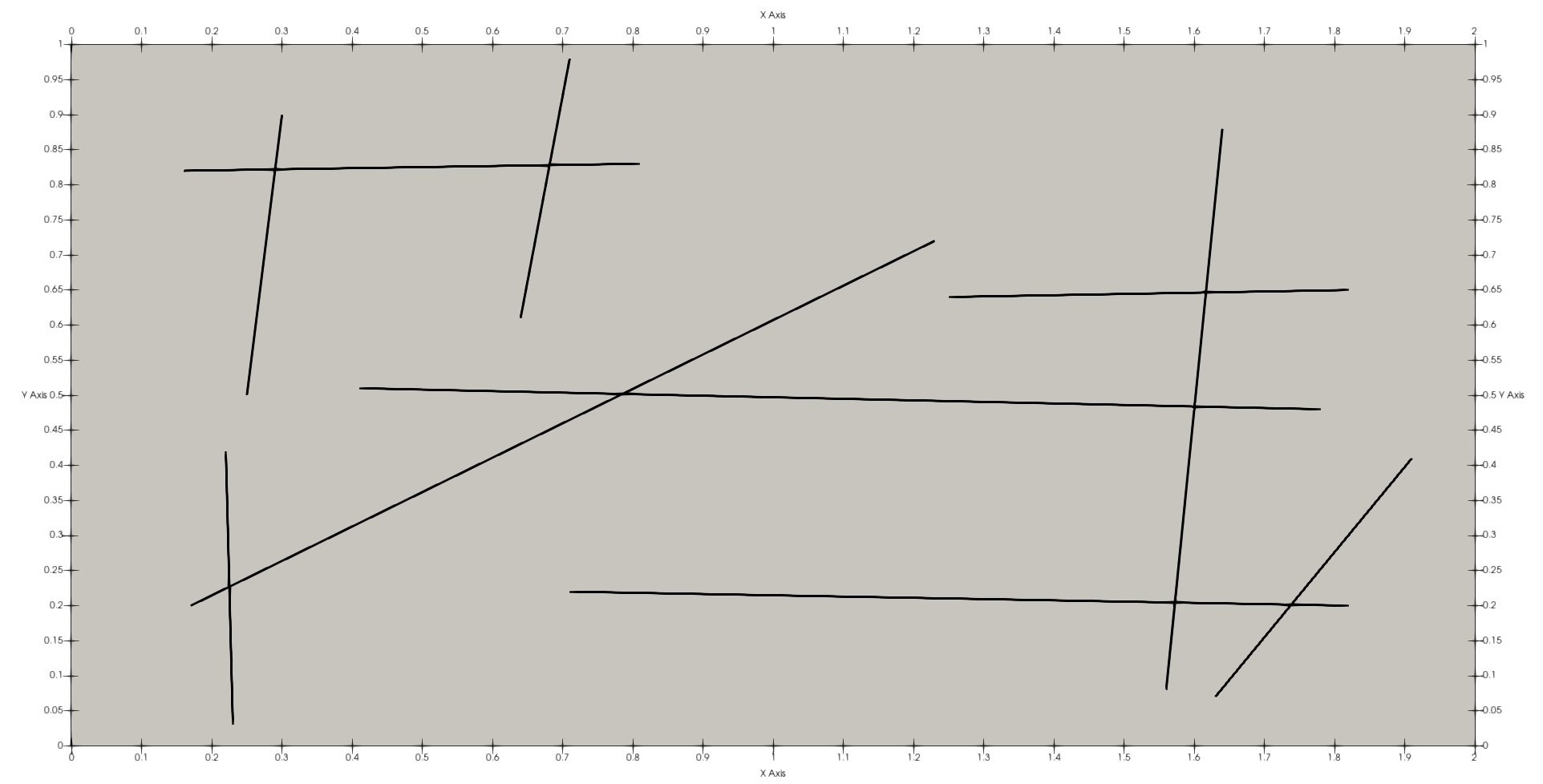
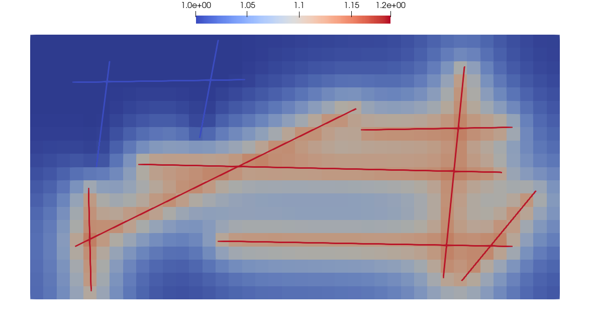
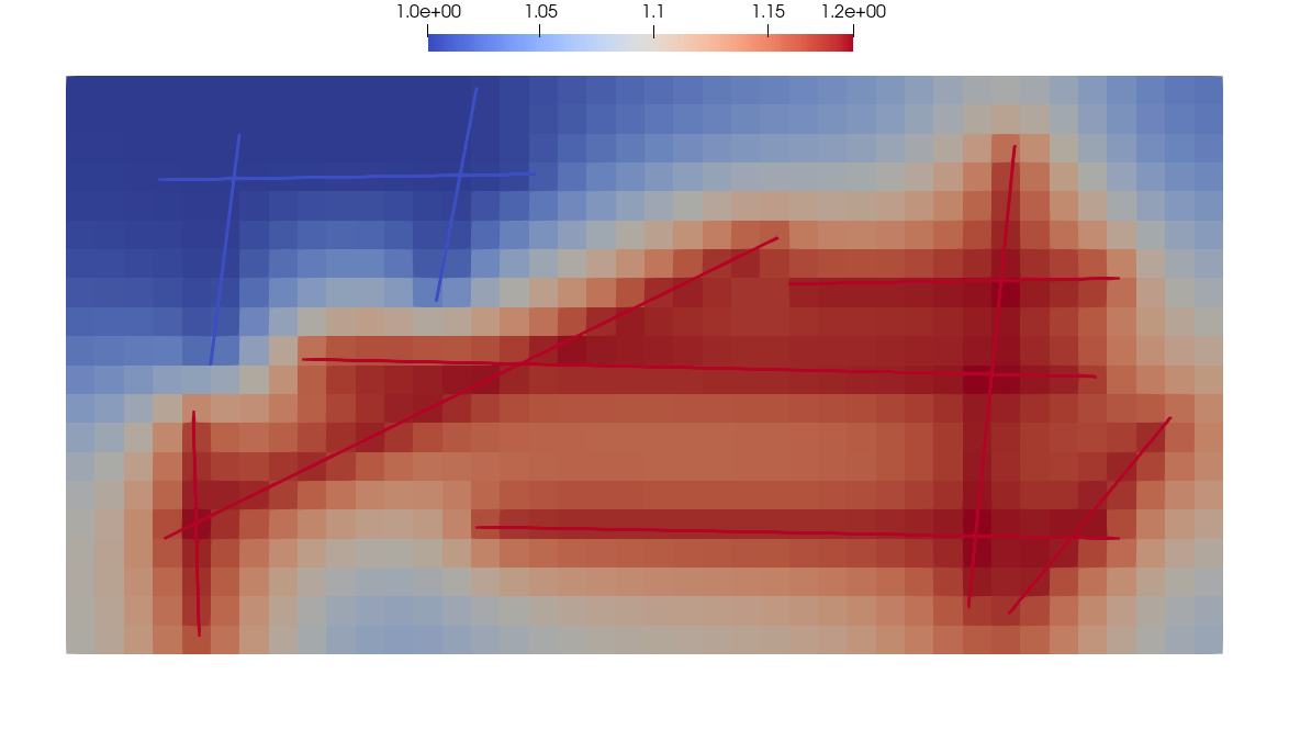
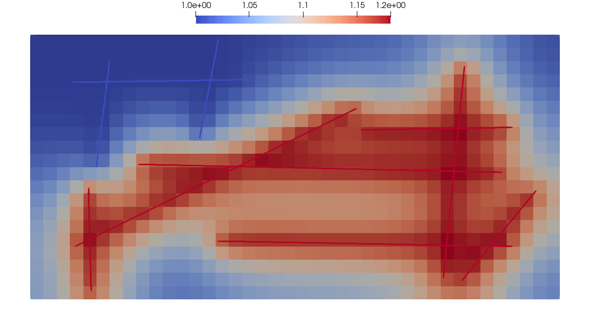
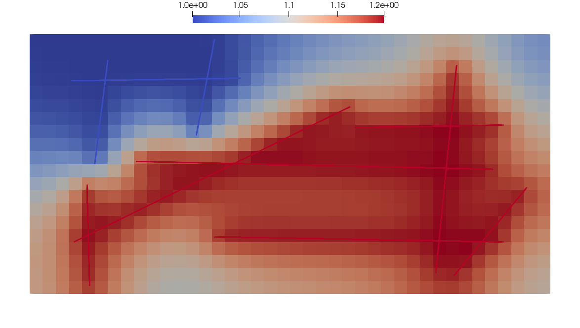
The problem is considered in domain with 10 fracture lines , (Figure 1). For domain , the fine grid is grid with square cells () and the coarse grid is grid with square cells (). For the lower-dimensional fracture domain , the fine grid contains cells, and the coarse grid contains cells. Lower-dimensional fractures are considered an overlaying continuum and approximated using embedded fracture model (EFM) [28, 53, 52]. The fine-scale approach is accurate for a sufficiently fine grid. We construct accurate multiscale basis functions in the NLMC method for coarse-scale approximation to incorporate complex flow behavior on a coarse grid model.
We set source term in fractures located in the coarse fracture cell related to the domain ). We set , and for with and and zero otherwise. As initial condition, we set () and perform simulations with .


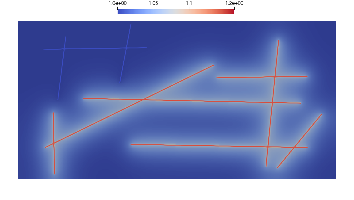
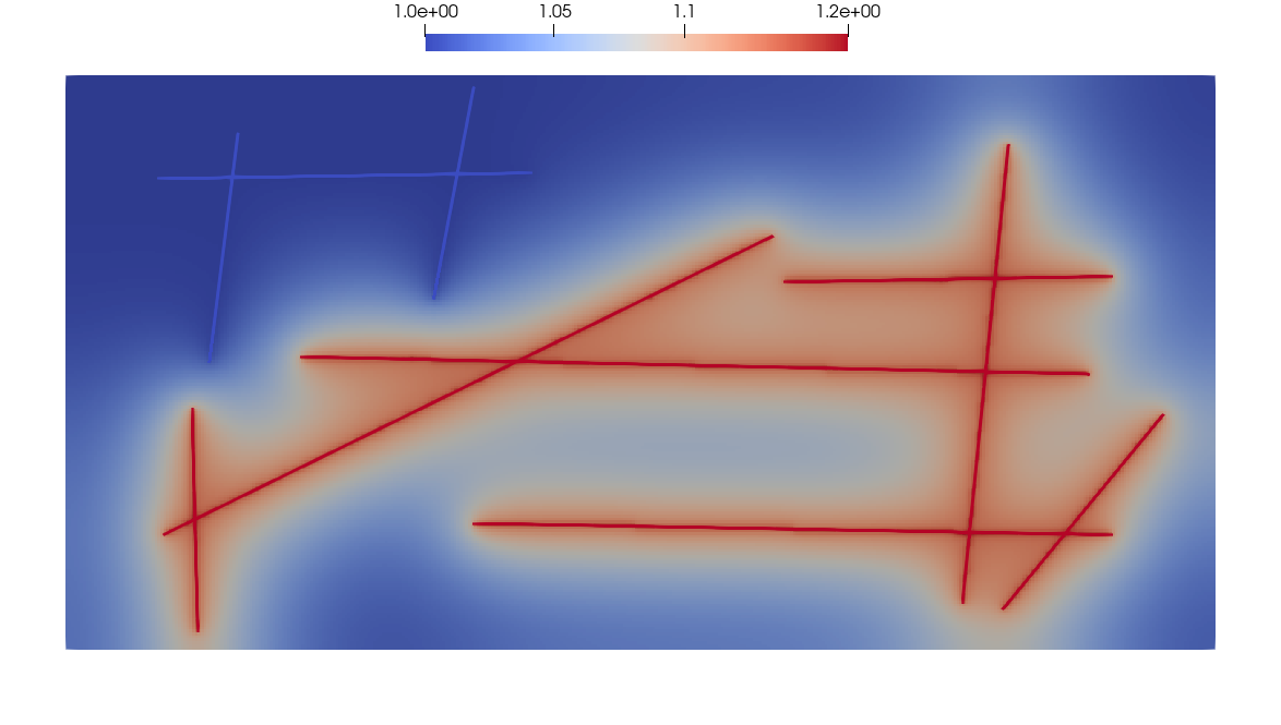
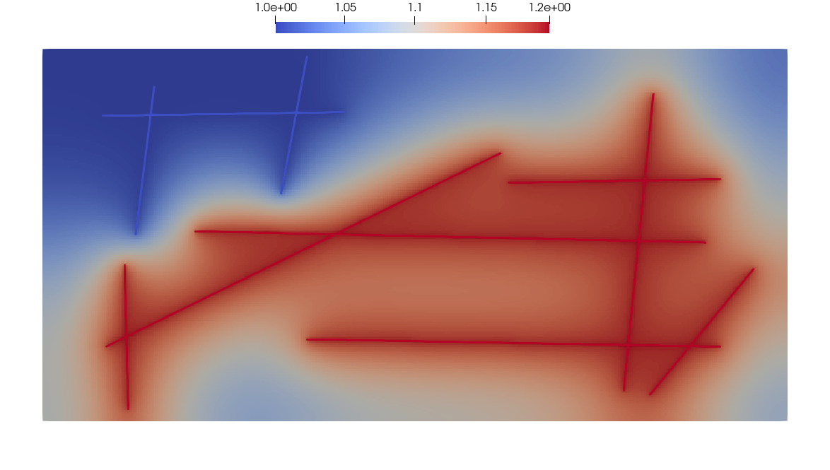
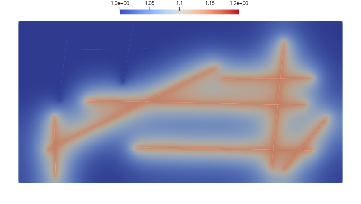
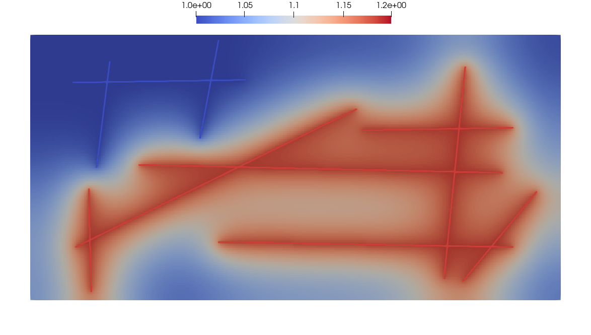

To perform a numerical investigation of the proposed Implicit and Implicit-Explicit schemes for finite-volume and multiscale approximations, we use the solution on the fine grid with using coupled scheme (implicit scheme (10) with ) as a reference solution. In Figure 2 and 3, we present a solution for two- and three–continuum media, respectively. The solution is shown at three time layers and (). In the coupled scheme, we solve a large coupled system of equations that have for a two-continuum problem (2C) and for a three-continuum problem (3C).
Next, we numerically study schemes for various time step sizes and with . We investigate the influence of the time step size on the method accuracy for coupled and decoupled schemes. We consider the following schemes:
- •
- •
We also consider three variations of decoupled schemes: L, D, and U-scheme. The schemes are based on the different additive representations of the operator (see (18), (16) and (19)) and related to the order of computations. Implementation is performed using the PETSc library [8], using a conjugate gradient (CG) iterative solver with ILU preconditioner. Simulations are performed on MacBook Pro (2.3 GHz Quad-Core Intel Core i7 with 32 GB 3733 MHz LPDDR4X).
5.1 Implicit-Explicit for fine-scale system
In this section, we consider a fine grid problem, where a finite-volume approximation is used to construct space approximation. We numerically investigate coupled and decoupled schemes.
| Implicit | ||
|---|---|---|
| (%) | (%) | |
| Im1 | ||
| 4 | 1.0059 | 17.9344 |
| 8 | 0.5217 | 9.7381 |
| 16 | 0.2673 | 5.0979 |
| 32 | 0.1375 | 2.6395 |
| 64 | 0.0719 | 1.3776 |
| 128 | 0.0391 | 0.7395 |
| Im2-CN | ||
| 4 | 0.0893 | 2.0623 |
| 8 | 0.0247 | 0.8536 |
| 16 | 0.0058 | 0.7281 |
| 32 | 0.0013 | 0.6634 |
| 64 | 0.0017 | 0.5349 |
| 128 | 0.0021 | 0.3577 |
| Im2-BDF | ||
| 4 | 0.5519 | 11.9551 |
| 8 | 0.1397 | 3.0781 |
| 16 | 0.0320 | 0.6910 |
| 32 | 0.0080 | 0.1791 |
| 64 | 0.0022 | 0.0589 |
| 128 | 0.0009 | 0.0308 |
| Implicit-Explicit | ||||||
|---|---|---|---|---|---|---|
| L | D | U | ||||
| (%) | (%) | (%) | (%) | (%) | (%) | |
| ImEx1 | ||||||
| 4 | 3.0290 | 100 | 3.4885 | 100 | 1.3912 | 21.9411 |
| 8 | 1.3841 | 34.6548 | 1.6220 | 39.9831 | 0.7023 | 11.9741 |
| 16 | 0.6551 | 14.2659 | 0.7578 | 16.0401 | 0.3522 | 6.2784 |
| 32 | 0.3201 | 6.6071 | 0.3655 | 7.3213 | 0.1782 | 3.2420 |
| 64 | 0.1605 | 3.2350 | 0.1816 | 3.5600 | 0.0919 | 1.6813 |
| 128 | 0.0828 | 1.6410 | 0.0929 | 1.7968 | 0.0489 | 0.8920 |
| ImEx2-CNAB | ||||||
| 4 | 4.5677 | 100 | 6.0503 | 100 | 3.7071 | 100 |
| 8 | 0.4268 | 81.8828 | 5.4027 | 100 | 0.3288 | 71.7085 |
| 16 | 0.1609 | 42.4335 | 1.8389 | 100 | 0.1331 | 45.1967 |
| 32 | 0.0631 | 15.446 | 0.2309 | 100 | 0.0722 | 20.8431 |
| 64 | 0.0163 | 1.7747 | 0.0337 | 8.4869 | 0.0496 | 4.1516 |
| 128 | 0.0086 | 0.3953 | 0.0010 | 0.3870 | 0.0402 | 0.9422 |
| ImEx2-SBDF | ||||||
| 4 | 2.8739 | 100 | 3.0840 | 91.0879 | 2.5372 | 100 |
| 8 | 0.6759 | 25.6489 | 0.8206 | 32.7378 | 0.3708 | 9.8857 |
| 16 | 0.2517 | 5.3571 | 0.3213 | 6.4609 | 0.0721 | 3.3658 |
| 32 | 0.1042 | 2.1288 | 0.1389 | 2.6478 | 0.0342 | 1.6021 |
| 64 | 0.0280 | 0.5888 | 0.0449 | 0.8388 | 0.0372 | 1.0167 |
| 128 | 0.0121 | 0.2169 | 0.0029 | 0.0729 | 0.0432 | 0.9162 |
| Implicit | ||
|---|---|---|
| (%) | (%) | |
| Im1 | ||
| 4 | 1.0600 | 16.3468 |
| 8 | 0.5687 | 9.2291 |
| 16 | 0.2974 | 4.9515 |
| 32 | 0.1548 | 2.5998 |
| 64 | 0.0818 | 1.3684 |
| 128 | 0.0449 | 0.7396 |
| Im2-CN | ||
| 4 | 0.0918 | 1.7399 |
| 8 | 0.0253 | 0.7161 |
| 16 | 0.0063 | 0.6049 |
| 32 | 0.0024 | 0.5508 |
| 64 | 0.0027 | 0.4443 |
| 128 | 0.0030 | 0.2978 |
| Im2-BDF | ||
| 4 | 0.4052 | 10.0464 |
| 8 | 0.1216 | 2.2998 |
| 16 | 0.0313 | 0.5631 |
| 32 | 0.0084 | 0.1577 |
| 64 | 0.0026 | 0.0580 |
| 128 | 0.0012 | 0.0332 |
| Implicit-Explicit | ||||||
|---|---|---|---|---|---|---|
| L | D | U | ||||
| (%) | (%) | (%) | (%) | (%) | (%) | |
| ImEx1 | ||||||
| 4 | 5.1618 | 100 | 5.6480 | 100 | 2.0955 | 33.2298 |
| 8 | 2.5859 | 47.0465 | 3.0596 | 55.8464 | 1.1479 | 19.1050 |
| 16 | 1.2739 | 21.7915 | 1.5668 | 26.6997 | 0.6052 | 10.2833 |
| 32 | 0.6324 | 10.5583 | 0.7912 | 13.1384 | 0.3139 | 5.3677 |
| 64 | 0.3179 | 5.2425 | 0.4001 | 6.5626 | 0.1630 | 2.7810 |
| 128 | 0.1625 | 2.6555 | 0.2044 | 3.3234 | 0.0862, | 1.4560 |
| ImEx2-CNAB | ||||||
| 4 | 6.4256 | 100 | 6.6215 | 100 | 4.5543 | 100 |
| 8 | 0.3956 | 70.6279 | 4.3660 | 100 | 1.3503 | 65.1615 |
| 16 | 0.1244 | 35.4564 | 1.4028 | 100 | 0.6573 | 39.1486 |
| 32 | 0.0639 | 12.8874 | 0.1987 | 100 | 0.3406 | 18.1321 |
| 64 | 0.0473 | 1.8030 | 0.0437 | 7.0812 | 0.1888 | 4.5650 |
| 128 | 0.0428 | 0.8537 | 0.0018 | 0.3221 | 0.1145 | 1.9190 |
| ImEx2-SBDF | ||||||
| 4 | 4.3465 | 100 | 4.7712 | 98.5998 | 3.7142 | 223.4047 |
| 8 | 0.6878 | 25.6575 | 1.1494 | 30.5044 | 1.3159 | 22.7793 |
| 16 | 0.1249 | 4.2209 | 0.4291 | 6.7873 | 0.5516 | 9.7356 |
| 32 | 0.0417 | 1.6920 | 0.1823 | 2.8165 | 0.2875 | 5.0038 |
| 64 | 0.0336 | 0.9427 | 0.0590 | 0.8991 | 0.1723 | 2.9180 |
| 128 | 0.0473 | 0.8639 | 0.0040 | 0.0873 | 0.1182 | 1.9514 |
To compare schemes, we calculate and energy relative errors in percentage at time
with
where is the reference solution (coupled Im1-scheme with ), and is the approximate solution using different schemes (Im1, Im2-CN, Im2-BDF, ImEx1, ImEx2-CNAB and ImEx2-SBDF) and and .
| Implicit | ||
|---|---|---|
| timetot | ||
| Im1 | ||
| 4 | 2.294 | 429.5 |
| 8 | 3.869 | 362.0 |
| 16 | 6.441 | 280.6 |
| 32 | 9.747 | 227.0 |
| 64 | 15.770 | 184.1 |
| 128 | 25.311 | 146.5 |
| Im2-CN | ||
| 4 | 1.450 | 359.7 |
| 8 | 2.605 | 278.1 |
| 16 | 4.558 | 227.1 |
| 32 | 7.653 | 184.2 |
| 64 | 12.412 | 146.5 |
| 128 | 20.322 | 117.9 |
| Im2-BDF | ||
| 4 | 1.582 | 391.3 |
| 8 | 2.985 | 316.1 |
| 16 | 4.948 | 244.2 |
| 32 | 8.404 | 201.6 |
| 64 | 13.563 | 160.4 |
| 128 | 22.015 | 129.7 |
| Implicit-Explicit | |||||
|---|---|---|---|---|---|
| timetot | time | time | |||
| ImEx1 | |||||
| 4 | 0.842 | 0.837 | 160.0 | 0.004 | 59.2 |
| 8 | 1.314 | 1.306 | 124.0 | 0.008 | 58.1 |
| 16 | 1.994 | 1.977 | 93.9 | 0.016 | 57.8 |
| 32 | 2.907 | 2.874 | 68.0 | 0.033 | 57.1 |
| 64 | 4.347 | 4.283 | 50.0 | 0.064 | 55.5 |
| 128 | 6.351 | 6.227 | 36.0 | 0.124 | 53.3 |
| ImEx2-CNAB | |||||
| 4 | 0.550 | 0.545 | 124.7 | 0.004 | 59.0 |
| 8 | 1.018 | 1.009 | 93.9 | 0.009 | 57.3 |
| 16 | 1.654 | 1.633 | 68.0 | 0.020 | 57.3 |
| 32 | 2.704 | 2.662 | 50.0 | 0.042 | 55.5 |
| 64 | 4.284 | 4.203 | 36.0 | 0.081 | 53.1 |
| 128 | 6.777 | 6.609 | 25.0 | 0.167 | 53.0 |
| ImEx2-SBDF | |||||
| 4 | 0.602 | 0.598 | 139.0 | 0.003 | 58.3 |
| 8 | 1.105 | 1.095 | 105.0 | 0.009 | 57.1 |
| 16 | 1.828 | 1.808 | 78.0 | 0.020 | 57.4 |
| 32 | 2.935 | 2.893 | 57.0 | 0.042 | 56.8 |
| 64 | 4.651 | 4.568 | 41.0 | 0.083 | 54.1 |
| 128 | 7.517 | 7.347 | 29.0 | 0.169 | 53.0 |
| Implicit | ||
|---|---|---|
| timetot | ||
| Im1 | ||
| 4 | 4.527 | 369.8 |
| 8 | 7.698 | 315.9 |
| 16 | 12.460 | 256.3 |
| 32 | 20.605 | 213.4 |
| 64 | 33.814 | 175.0 |
| 128 | 53.684 | 140.1 |
| Im2-CN | ||
| 4 | 2.833 | 314.7 |
| 8 | 5.452 | 256.1 |
| 16 | 9.701 | 213.3 |
| 32 | 16.706 | 175.0 |
| 64 | 27.507 | 140.1 |
| 128 | 46.016 | 115.4 |
| Im2-BDF | ||
| 4 | 3.069 | 336.0 |
| 8 | 5.976 | 280.4 |
| 16 | 10.483 | 229.3 |
| 32 | 18.220 | 191.9 |
| 64 | 29.982 | 154.6 |
| 128 | 49.034 | 125.1 |
| Implicit-Explicit | |||||||
|---|---|---|---|---|---|---|---|
| timetot | time | time | time | ||||
| ImEx1 | |||||||
| 4 | 0.767 | 0.042 | 7.0 | 0.720 | 139.0 | 0.004 | 59.2 |
| 8 | 1.267 | 0.074 | 6.0 | 1.185 | 113.6 | 0.008 | 59.0 |
| 16 | 2.012 | 0.130 | 5.0 | 1.865 | 89.0 | 0.016 | 58.3 |
| 32 | 3.029 | 0.213 | 4.0 | 2.783 | 66.0 | 0.032 | 57.0 |
| 64 | 4.645 | 0.429 | 4.0 | 4.151 | 49.0 | 0.064 | 55.9 |
| 128 | 6.858 | 0.698 | 3.0 | 6.037 | 35.0 | 0.122 | 53.2 |
| ImEx2-CNAB | |||||||
| 4 | 0.584 | 0.080 | 6.0 | 0.499 | 113.7 | 0.004 | 59.3 |
| 8 | 1.128 | 0.179 | 5.0 | 0.938 | 88.9 | 0.009 | 57.6 |
| 16 | 1.953 | 0.370 | 4.0 | 1.563 | 66.0 | 0.020 | 57.0 |
| 32 | 3.358 | 0.758 | 4.0 | 2.558 | 49.0 | 0.041 | 55.7 |
| 64 | 5.704 | 1.525 | 3.0 | 4.097 | 35.0 | 0.081 | 53.2 |
| 128 | 9.601 | 2.928 | 3.0 | 6.512 | 25.0 | 0.159 | 52.9 |
| ImEx2-SBDF | |||||||
| 4 | 0.625 | 0.085 | 7.0 | 0.536 | 124.0 | 0.004 | 59.0 |
| 8 | 1.217 | 0.189 | 6.0 | 1.019 | 98.9 | 0.009 | 58.3 |
| 16 | 2.139 | 0.394 | 5.0 | 1.724 | 75.0 | 0.019 | 57.1 |
| 32 | 3.613 | 0.749 | 4.0 | 2.822 | 56.0 | 0.041 | 56.5 |
| 64 | 6.126 | 1.534 | 3.0 | 4.509 | 40.0 | 0.081 | 54.3 |
| 128 | 10.389 | 3.016 | 3.0 | 7.211 | 29.0 | 0.161 | 53.0 |
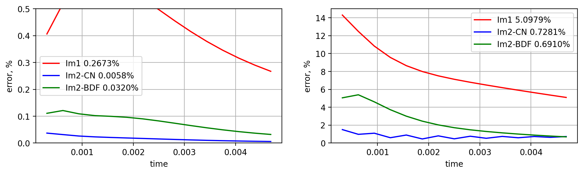
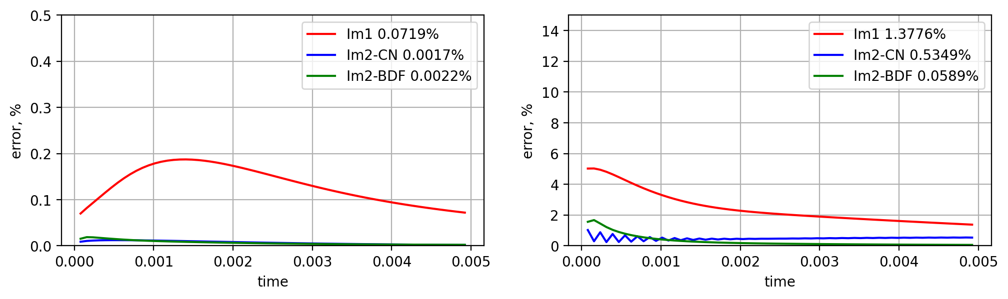
In Tables 1 and 2, we present errors for two and three-continuum media, respectively. We show an error in percentage at the final time. We observe the following convergence behavior of the proposed schemes from the result. For the three-level schemes, we have a smaller error. For example, in Table 1 for a two-continuum test problem and in Table 2 for a three-continuum test problem, we have less than 1% of energy error for time steps in the two-level scheme, Im1. For three-level implicit schemes, we have less than 1% energy error for and time steps in Im2-CN and Im2-BDF, respectively. In the uncoupled case (D-schemes) for two-continuum case in Table 1, we have near 2% of energy error in two-level decoupled scheme (ImEx1) for and for three-level decoupled scheme (ImEx2-SBDF). For the three-continuum case in Table 2, we have nearly 3% of energy error in the first-order decoupled scheme (ImEx1) for and for second-order decoupled scheme (ImEx2-SBDF). Therefore, we can use a 4-times bigger time step size in the second-order schemes.
Next, we compare the coupled and decoupled schemes. For the two-level schemes in Table 1, we have nearly 1% of energy error for time steps in both coupled and decoupled schemes (Im1 and ImEx1-U). Moreover, we observe that the U-decoupling scheme gives better results compared with L and D-schemes in ImEx1. We see that continuum order matters in calculations: (1) It is better to use previous continuum solution information in calculations, and (2) First, calculate the continuum with higher permeability or faster flow. For the second-order decoupled scheme, we observe that the errors are smaller for the L-scheme in ImEx2-CNAB and ImEx2-SBDF. However, it is better to use a U-scheme for a smaller time step size. Moreover, we also observe that the D-scheme gives more considerable errors for ImEx2-CNAB with fewer time steps and can lead to a big energy error. By comparing the coupled and uncoupled schemes of the three-level, we observe a more significant influence on the method accuracy. For example, we can use in the Im2-BDF coupled scheme to obtain near 1% of energy error, but in the ImEx2-SBDF decoupled scheme, we should use .
In Figure 4, we depicted the dynamics of the error by time. We show the errors in and energy norms for on the first row and for on the second row. The figures illustrate a good performance of the second-order schemes compared with a first-order for a coupled case of calculations. We observe a well-known zigzag behavior of the Crank-Nicholson scheme at the beginning of simulations. When we use a more significant time step size (, first row in Figure 4), we observe more minor errors for the Im2-CN scheme compared with the Im2-BDF for both two-continuum and three-continuum test problems. However, for , we follow a more minor error for the Im2-BDF scheme. Finally, we discuss the computational performance of the presented schemes for the fine grid problem. We show the total time of computations in seconds with an average number of iterations for the preconditioned conjugate gradient method in Tables 3 and 4. In both tables, timetot denotes the total time of computations for coupled schemes for given and time is the total time of calculations related to the -continuum in decoupled schemes, for two-continuum test and for three-continuum test. denotes an average number of iterations in one time layer, and is related to the -continuum in the decoupled schemes. For the decoupled schemes, we have the same computational time and number of iterations in L, D, and U-schemes. Therefore, the results in Tables 3 and 4 are presented for U-scheme. To compare the computational efficiency, we present the reference solution’s time and number of iterations.
-
•
Two-continuum media (2C): , time sec. and using coupled (Im1) scheme for .
-
•
Three-continuum media (3C): , time sec. and using coupled (Im1) scheme for .
We observe the same computation time for first- and second-order schemes from the presented results. For the coupled schemes for the two-continuum test, we have sec for and sec for . In the coupled case on each time iteration, we solve the linear system with and unknowns for two and three-continuum tests, respectively. In the decoupled case, we decoupled the system into systems with smaller sizes that are faster to solve. We have times faster calculations for the two-continuum test with nearly sec for and sec for . In the three-continuum cases, we obtain better results with sec for the coupled schemes and sec for decoupled implicit-explicit schemes for . Then, we have times faster calculations for the two-level scheme and times faster calculations for the second order scheme. The computational time is reduced due to the small size of the system in the decoupled case that requires a smaller number of iterations. The implicit-explicit schemes also decouple continuums and significantly affect the number of iterations. Furthermore, we observe that the most time is taken by a first continuum defined in in 2C test and by second continuum in 3C test. The fracture continuum requires a more significant number of iterations in both test cases. However, the time of calculations is very short due to the size of the fracture continuum system compared with the continuum defined in with for 2C and for 3C.
5.2 Implicit-Explicit for coarse-scale system
This section considers a coarse grid problem constructed with NLMC approximation. Similar to the previous subsection, we numerically investigate coupled and decoupled schemes. In this case, we are more interested in the coarse grid system errors; however, we can reconstruct the fine-scale solution using the constructed projection operator. We use a relative error in percentage at time on fine and coarse grids to compare the proposed schemes.
with
where is the reference solution, is the coarse grid reference solution (average over coarse cell ), is the multiscale solution on the fine grid, and is the multiscale solution on the coarse grid.
| Implicit schemes + Ms | ||||||||||
|---|---|---|---|---|---|---|---|---|---|---|
| Ms-Im1 | ||||||||||
| 4 | 83.9536 | 86.4985 | 3.2716 | 1.0142 | 1.2637 | 0.9429 | 1.0209 | 0.9389 | 1.0054 | 0.9390 |
| 8 | 85.4075 | 87.7092 | 3.1621 | 0.5784 | 0.9254 | 0.4864 | 0.5502 | 0.4812 | 0.5201 | 0.4813 |
| 16 | 85.8038 | 88.0360 | 3.1315 | 0.3608 | 0.8098 | 0.2491 | 0.3218 | 0.2431 | 0.2664 | 0.2431 |
| 32 | 85.9576 | 88.1630 | 3.1232 | 0.2584 | 0.7769 | 0.1289 | 0.2286 | 0.1221 | 0.1397 | 0.1221 |
| 64 | 85.9905 | 88.1897 | 3.1209 | 0.2122 | 0.7681 | 0.0691 | 0.1982 | 0.0613 | 0.0805 | 0.0613 |
| 128 | 85.8956 | 88.1091 | 3.1202 | 0.1916 | 0.7658 | 0.0401 | 0.1899 | 0.0311 | 0.0566 | 0.0310 |
| Ms-Im2-CN | ||||||||||
| 4 | 81.6139 | 84.5647 | 3.6606 | 1.9931 | 1.9531 | 1.9128 | 1.7926 | 1.9046 | 1.7834 | 1.9048 |
| 8 | 93.0646 | 94.1468 | 3.4462 | 1.4434 | 1.5967 | 1.4458 | 1.4083 | 1.4442 | 1.3965 | 1.4446 |
| 16 | 99.4061 | 99.4906 | 3.4133 | 1.3131 | 1.5556 | 1.3494 | 1.3653 | 1.3508 | 1.3532 | 1.3513 |
| 32 | 100.006 | 100.012 | 3.4074 | 1.2780 | 1.5548 | 1.3282 | 1.3659 | 1.3308 | 1.3538 | 1.3313 |
| 64 | 99.9998 | 99.9984 | 3.4067 | 1.2671 | 1.5586 | 1.3234 | 1.3709 | 1.3265 | 1.3589 | 1.3270 |
| 128 | 100.000 | 100.001 | 3.4068 | 1.2631 | 1.5615 | 1.3223 | 1.3745 | 1.3256 | 1.3625 | 1.3261 |
| Ms-Im2-BDF | ||||||||||
| 4 | 81.9196 | 84.7940 | 5.1153 | 3.8363 | 4.1302 | 3.7634 | 4.0598 | 3.7587 | 4.0565 | 3.7589 |
| 8 | 84.5305 | 86.9679 | 3.4730 | 1.4733 | 1.6554 | 1.3504 | 1.4728 | 1.3418 | 1.4618 | 1.3418 |
| 16 | 85.3065 | 87.6165 | 3.1968 | 0.7177 | 0.9912 | 0.5817 | 0.6502 | 0.5723 | 0.6244 | 0.5722 |
| 32 | 85.6212 | 87.8796 | 3.1411 | 0.4220 | 0.8223 | 0.2801 | 0.3486 | 0.2706 | 0.2977 | 0.2704 |
| 64 | 85.6438 | 87.8975 | 3.1268 | 0.2907 | 0.7799 | 0.1431 | 0.2365 | 0.1334 | 0.1519 | 0.1332 |
| 128 | 85.3894 | 87.6826 | 3.1225 | 0.2302 | 0.7691 | 0.0779 | 0.2009 | 0.0678 | 0.0865 | 0.0676 |


In NLMC approximation, we significantly influence the local domain size used in multiscale basis calculations to the method’s accuracy. This study considers a two-continuum test problem to choose an optimal number of oversampling layers in basis calculations. In Table 5, we present the influence of the number of oversampling layers ( and ) on the method accuracy for the fine and coarse grid multiscale solutions, and at the final time. In Figure 5, we present fine grid and coarse grid multiscale solutions at the final time on the first and second rows, respectively. Combining the visual representation of the solution from Figure 5 and relative errors from Table 5, we can observe how several oversamplings affect the accuracy. Here, we observe that one cannot obtain a solution for the NLMC method by using one oversampling layer in local domain construction. When we use oversampling layers, we have a good approximation of the coarse grid solution. However, two oversampling layers are not enough for good fine-grid resolution of the solution. We should use five oversampling layers to obtain smooth results on the fine grid with a small error. However, because we are more interested in the coarse grid model, we can say that the solution is good with less than one % of error if we use three oversampling layers. We should mention that the number of oversampling layers directly affects the time of multiscale basis calculations. However, the calculations are performed in a parallel way, i.e., for each local domain independently.

Next, in Figures 6 and 7, we depict the solution of the coarse grid system for two and three-continuum test problems, respectively. We use an NLMC approximation with three oversampling layers on a coarse grid. The resulting unknowns on the coarse grid are and for 2C and 3C tests in the coupled scheme. The results are shown for the coupled scheme using the two-level coupled scheme (Ms-Im1) with and represented for , and . For the 2C test in Figure 6, we have and for and , respectively. For the 3C test in Figure 7, we have and for and , respectively. Solution time is 0.9 sec for 2C and 2.8 for 3C using on coarse grid with and for 2C and 3C tests, respectively. We have a speedy solution compared to the fine grid system using the same scheme (Im1). On the fine grid, we have 25.3 sec for 2C and 53.6 for 3C for .
| Implicit schemes + Ms | ||
|---|---|---|
| Ms-Im1 | ||
| 4 | 1.2637 | 0.9429 |
| 8 | 0.9254 | 0.4864 |
| 16 | 0.8098 | 0.2491 |
| 32 | 0.7769 | 0.1289 |
| 64 | 0.7681 | 0.0691 |
| 128 | 0.7658 | 0.0401 |
| Ms-Im2-CN | ||
| 4 | 1.9531 | 1.9128 |
| 8 | 1.5967 | 1.4458 |
| 16 | 1.5556 | 1.3494 |
| 32 | 1.5548 | 1.3282 |
| 64 | 1.5586 | 1.3234 |
| 128 | 1.5615 | 1.3223 |
| Ms-Im2-BDF | ||
| 4 | 4.1302 | 3.7634 |
| 8 | 1.6554 | 1.3504 |
| 16 | 0.9912 | 0.5817 |
| 32 | 0.8223 | 0.2801 |
| 64 | 0.7799 | 0.1431 |
| 128 | 0.7691 | 0.0779 |
| Implicit-Explicit schemes + Ms | ||||||
|---|---|---|---|---|---|---|
| L | D | U | ||||
| Ms-ImEx1 | ||||||
| 4 | 2.9032 | 2.5825 | 3.1320 | 2.8103 | 1.4203 | 1.1282 |
| 8 | 1.4942 | 1.1840 | 1.5961 | 1.2948 | 0.9791 | 0.5725 |
| 16 | 0.9794 | 0.5651 | 1.0118 | 0.6126 | 0.8250 | 0.2897 |
| 32 | 0.8218 | 0.2790 | 0.8304 | 0.3002 | 0.7808 | 0.1485 |
| 64 | 0.7798 | 0.1424 | 0.7819 | 0.1522 | 0.7691 | 0.0786 |
| 128 | 0.7689 | 0.0761 | 0.7695 | 0.0808 | 0.7661 | 0.0446 |
| Ms-ImEx2-CNAB | ||||||
| 4 | 4.7519 | 4.0709 | 9.8183 | 8.4932 | 2.0231 | 1.6289 |
| 8 | 1.1839 | 0.7780 | 3.6943 | 3.0293 | 0.8564 | 0.3135 |
| 16 | 0.8151 | 0.2601 | 0.8531 | 0.3401 | 0.7695 | 0.0749 |
| 32 | 0.7770 | 0.1277 | 0.7806 | 0.1456 | 0.7652 | 0.0283 |
| 64 | 0.7680 | 0.0684 | 0.7689 | 0.0770 | 0.7649 | 0.0161 |
| 128 | 0.7658 | 0.0409 | 0.7661 | 0.0449 | 0.7648 | 0.0154 |
| Ms-ImEx2-SBDF | ||||||
| 4 | 6.0360 | 5.4880 | 6.7632 | 6.2137 | 2.2684 | 1.9512 |
| 8 | 1.6974 | 1.3915 | 1.8356 | 1.5321 | 0.9277 | 0.4841 |
| 16 | 0.9805 | 0.5657 | 1.0122 | 0.6114 | 0.7993 | 0.2168 |
| 32 | 0.8179 | 0.2689 | 0.8257 | 0.2886 | 0.7750 | 0.1190 |
| 64 | 0.7785 | 0.1364 | 0.7804 | 0.1455 | 0.7680 | 0.0680 |
| 128 | 0.7687 | 0.0743 | 0.7692 | 0.0786 | 0.7659 | 0.0422 |
| Implicit schemes + Ms | ||
|---|---|---|
| Ms-Im1 | ||
| 4 | 1.3455 | 1.0230 |
| 8 | 1.0043 | 0.5469 |
| 16 | 0.8797 | 0.2858 |
| 32 | 0.8426 | 0.1497 |
| 64 | 0.8325 | 0.0814 |
| 128 | 0.8299 | 0.0490 |
| Ms-Im2-CN | ||
| 4 | 2.7302 | 2.9878 |
| 8 | 3.3793 | 3.4420 |
| 16 | 3.5427 | 3.5034 |
| 32 | 3.5863 | 3.5040 |
| 64 | 3.6011 | 3.4994 |
| 128 | 3.6070 | 3.4961 |
| Ms-Im2-BDF | ||
| 4 | 4.7068 | 4.4402 |
| 8 | 2.0320 | 1.7732 |
| 16 | 1.1619 | 0.7808 |
| 32 | 0.9174 | 0.3795 |
| 64 | 0.8525 | 0.1955 |
| 128 | 0.8356 | 0.1077 |
| Implicit-Explicit schemes + Ms | ||||||
|---|---|---|---|---|---|---|
| L | D | U | ||||
| Ms-ImEx1 | ||||||
| 4 | 5.0779 | 4.7829 | 5.4451 | 5.1400 | 2.0967 | 1.8501 |
| 8 | 2.6295 | 2.3841 | 2.9927 | 2.7472 | 1.3463 | 1.0186 |
| 16 | 1.4840 | 1.1777 | 1.6917 | 1.4104 | 1.0015 | 0.5414 |
| 32 | 1.0311 | 0.5886 | 1.1169 | 0.7179 | 0.8790 | 0.2845 |
| 64 | 0.8849 | 0.2997 | 0.9123 | 0.3678 | 0.8428 | 0.1515 |
| 128 | 0.8441 | 0.1575 | 0.8518 | 0.1924 | 0.8328 | 0.0848 |
| Ms-ImEx2-CNAB | ||||||
| 4 | 7.9192 | 7.3925 | 10.8835 | 10.0329 | 3.4384 | 3.1184 |
| 8 | 1.0533 | 0.5766 | 3.4144 | 2.8888 | 1.5138 | 1.1977 |
| 16 | 0.8407 | 0.1345 | 0.9445 | 0.4295 | 1.0113 | 0.5502 |
| 32 | 0.8315 | 0.0658 | 0.8537 | 0.1997 | 0.8728 | 0.2596 |
| 64 | 0.8295 | 0.0405 | 0.8355 | 0.1067 | 0.8386 | 0.1213 |
| 128 | 0.8291 | 0.0313 | 0.8308 | 0.0634 | 0.8307 | 0.0555 |
| Ms-ImEx2-SBDF | ||||||
| 4 | 10.7971 | 10.2690 | 10.4765 | 9.9767 | 2.3070 | 2.0212 |
| 8 | 1.9309 | 1.6661 | 2.5572 | 2.3095 | 1.1612 | 0.7747 |
| 16 | 1.0026 | 0.5421 | 1.2120 | 0.8478 | 0.8713 | 0.2571 |
| 32 | 0.8676 | 0.2488 | 0.9243 | 0.3948 | 0.8356 | 0.1038 |
| 64 | 0.8388 | 0.1278 | 0.8535 | 0.1995 | 0.8298 | 0.0449 |
| 128 | 0.8318 | 0.0735 | 0.8358 | 0.1088 | 0.8288 | 0.0251 |
Tables 6 and 7 show multiscale method errors at final time for two and three-continuum test problems, respectively. We observe the convergence behavior of the proposed Implicit and Implicit-Explicit schemes for multiscale approximation from the result. We observe excellent performance on the coarse grid approximation using the NLMC method for the first-order coupled and decoupled schemes. We can use fewer time steps and a coarse grid formulation to produce an accurate solution. For example, we have near 0.5 % of error using coupled Ms-Im1 scheme and decoupled version Ms-imEx1 using only eight time steps for 2C test (see Table 6). However, for both two and three-continuum tests, we observe a lousy performance of the second-order coupled scheme based on the Crank-Nicolson approximation (Ms-Im2-CN), where we have fundamental error % for 2C and % for 3C for . However, we can obtain good results using decoupled implicit-explicit variation (Ms-Im2-CNAB-D) with % for 2C and % for 3C for . Furthermore, we can obtain a perfect solution using only eight-time steps with less than one percent of error using the Ms-Im2-CNAB-L scheme. For the coupled Ms-Im2-BDF scheme and decoupled Ms-ImEx2-SBDF schemes, we obtain a little bit better results in decoupled case with near 0.5 % of error using in Ms-ImEx2-SBDF and using in Ms-Im2-BDF in 2C test. In 3C test, we observe a similar behavior with near 0.8 % of error using in Ms-ImEx2-SBDF and using in Ms-Im2-BDF. By comparing the L, D, and U versions of schemes, we see that the U-scheme works better for Ms-ImEx1 and Ms-ImEx2-SBDF schemes.
| Implicit + Ms | ||
|---|---|---|
| timetot | ||
| Ms-Im1 | ||
| 4 | 0.057 | 15.0 |
| 8 | 0.094 | 14.0 |
| 16 | 0.160 | 13.9 |
| 32 | 0.252 | 14.0 |
| 64 | 0.460 | 13.8 |
| 128 | 0.902 | 13.4 |
| Ms-Im2-CN | ||
| 4 | 0.047 | 14.0 |
| 8 | 0.070 | 13.7 |
| 16 | 0.119 | 14.0 |
| 32 | 0.214 | 13.6 |
| 64 | 0.403 | 13.3 |
| 128 | 0.752 | 13.0 |
| Ms-Im2-BDF | ||
| 4 | 0.047 | 15.0 |
| 8 | 0.071 | 14.0 |
| 16 | 0.127 | 13.9 |
| 32 | 0.215 | 13.8 |
| 64 | 0.402 | 13.6 |
| 128 | 0.754 | 13.0 |
| Implicit-Explicit + Ms | |||||
|---|---|---|---|---|---|
| timetot | time | time | |||
| Ms-ImEx1 | |||||
| 4 | 0.004 | 0.003 | 3.0 | 0.0007 | 14.0 |
| 8 | 0.009 | 0.007 | 3.0 | 0.0016 | 14.0 |
| 16 | 0.019 | 0.016 | 3.0 | 0.0032 | 14.0 |
| 32 | 0.030 | 0.023 | 2.0 | 0.0066 | 14.0 |
| 64 | 0.058 | 0.045 | 2.0 | 0.0129 | 13.9 |
| 128 | 0.120 | 0.095 | 2.0 | 0.0259 | 13.6 |
| Ms-ImEx2-CNAB | |||||
| 4 | 0.004 | 0.003 | 3.0 | 0.0007 | 14.0 |
| 8 | 0.009 | 0.008 | 3.0 | 0.0016 | 14.0 |
| 16 | 0.017 | 0.013 | 2.0 | 0.0037 | 14.0 |
| 32 | 0.036 | 0.028 | 2.0 | 0.0075 | 13.9 |
| 64 | 0.072 | 0.057 | 2.0 | 0.0151 | 13.8 |
| 128 | 0.151 | 0.122 | 2.0 | 0.0289 | 12.4 |
| Ms-ImEx2-SBDF | |||||
| 4 | 0.004 | 0.003 | 3.0 | 0.0007 | 14.0 |
| 8 | 0.009 | 0.008 | 3.0 | 0.0017 | 14.0 |
| 16 | 0.017 | 0.013 | 2.0 | 0.0036 | 14.0 |
| 32 | 0.037 | 0.029 | 2.0 | 0.0075 | 14.0 |
| 64 | 0.074 | 0.058 | 2.0 | 0.0155 | 13.8 |
| 128 | 0.146 | 0.116 | 2.0 | 0.0299 | 13.2 |
| Implicit + Ms | ||
|---|---|---|
| timetot | ||
| Ms-Im1 | ||
| 4 | 0.391 | 15.0 |
| 8 | 0.340 | 14.0 |
| 16 | 0.531 | 14.0 |
| 32 | 0.839 | 13.9 |
| 64 | 1.513 | 13.6 |
| 128 | 2.800 | 13.1 |
| Ms-Im2-CN | ||
| 4 | 0.240 | 14.0 |
| 8 | 0.321 | 14.0 |
| 16 | 0.483 | 14.0 |
| 32 | 0.789 | 13.6 |
| 64 | 1.427 | 13.2 |
| 128 | 2.438 | 12.0 |
| Ms-Im2-BDF | ||
| 4 | 0.241 | 15.0 |
| 8 | 0.321 | 14.0 |
| 16 | 0.485 | 14.0 |
| 32 | 0.820 | 13.8 |
| 64 | 1.416 | 13.4 |
| 128 | 2.596 | 13.0 |
| Implicit-Explicit + Ms | |||||||
|---|---|---|---|---|---|---|---|
| timetot | time | time | time | ||||
| Ms-ImEx1 | |||||||
| 4 | 0.006 | 0.002 | 1.0 | 0.004 | 3.0 | 0.0008 | 14.0 |
| 8 | 0.013 | 0.004 | 1.0 | 0.008 | 3.0 | 0.0016 | 14.0 |
| 16 | 0.026 | 0.008 | 1.0 | 0.014 | 2.6 | 0.0032 | 14.0 |
| 32 | 0.047 | 0.016 | 1.0 | 0.024 | 2.0 | 0.0065 | 14.0 |
| 64 | 0.094 | 0.032 | 1.0 | 0.048 | 2.0 | 0.0129 | 13.9 |
| 128 | 0.188 | 0.064 | 1.0 | 0.097 | 2.0 | 0.0258 | 13.7 |
| Ms-ImEx2-CNAB | |||||||
| 4 | 0.006 | 0.002 | 1.0 | 0.003 | 3.0 | 0.0007 | 14.0 |
| 8 | 0.015 | 0.005 | 1.0 | 0.007 | 2.6 | 0.0017 | 14.0 |
| 16 | 0.030 | 0.011 | 1.0 | 0.015 | 2.0 | 0.0036 | 14.0 |
| 32 | 0.047 | 0.016 | 1.0 | 0.024 | 2.0 | 0.0065 | 13.9 |
| 64 | 0.094 | 0.032 | 1.0 | 0.048 | 2.0 | 0.0129 | 13.7 |
| 128 | 0.188 | 0.064 | 1.0 | 0.097 | 2.0 | 0.0258 | 12.3 |
| Ms-ImEx2-SBDF | |||||||
| 4 | 0.006 | 0.002 | 1.0 | 0.003 | 3.0 | 0.0007 | 14.0 |
| 8 | 0.016 | 0.005 | 1.0 | 0.008 | 3.0 | 0.0017 | 14.0 |
| 16 | 0.029 | 0.011 | 1.0 | 0.014 | 2.0 | 0.0036 | 14.0 |
| 32 | 0.060 | 0.022 | 1.0 | 0.030 | 2.0 | 0.0075 | 14.0 |
| 64 | 0.138 | 0.051 | 1.0 | 0.069 | 2.0 | 0.0172 | 13.8 |
| 128 | 0.267 | 0.101 | 1.0 | 0.133 | 2.0 | 0.0323 | 13.3 |
Finally, we discuss the computational performance of the presented combination of the time and space approximation schemes, where we have a substantial computational time reduction based on the coarse grid calculations using the NLMC method. Moreover, we can decouple a system and use a more significant time step size using presented Implicit-Explicit time approximation schemes. Similarly to the fine grid calculations, we present the total time of computations in seconds with an average number of iterations for the preconditioned conjugate gradient method in Tables 8 and 9. For the decoupled schemes, the results are presented for U-scheme. For the coupled first-order scheme (Im1), we have the following:
-
•
Two-continuum media (2C):
-
–
Reference solution with (fine grid) with (Im1): time sec. and .
-
–
Fine-scale solution with (fine grid) with (Im1): time sec. and .
-
–
Multiscale solution with (coarse grid) with (Im1): time sec. and .
-
–
-
•
Three-continuum media (3C):
-
–
Reference solution with (fine grid) with (Im1): time sec. and
-
–
Fine-scale solution with (fine grid) with (Im1): time sec. and .
-
–
Multiscale solution with (coarse grid) with (Im1): time sec. and .
-
–
By constructing the accurate coarse-scale approximation, we reduce the size of the system significantly with 28.1 and 19.2 times faster calculations compared with a fine-scale solution with the same time step size ().
Moreover, from the Tables 8 and 9, we observe a significant influence of the decoupling to the time of computations. For , we have for the two-continuum test (2C):
-
•
Fine-scale solution with (fine grid):
-
–
Coupled scheme (Im2-BDF): time sec. with .
-
–
Decoupled scheme (ImEx2-SBDF): time sec. with and .
-
–
-
•
Multiscale solution with (coarse grid):
-
–
Coupled scheme (Ms-Im2-BDF): time sec. with .
-
–
Decoupled scheme (Ms-ImEx2-SBDF): time sec. with and .
-
–
In a second-order scheme with , we obtain a 2.7 times faster solution on the fine grid for the decoupled system and five times faster solution on the coarse grid with % of error compared with a reference solution. We also observe a significant reduction in the number of iterations for the continuum in , significantly influencing the solution time.
For the three-continuum media (3C):
-
•
Fine-scale solution with (fine grid):
-
–
Coupled scheme (Im2-BDF): time sec. with .
-
–
Decoupled scheme (ImEx2-SBDF): time sec. with , and .
-
–
-
•
Multiscale solution with (coarse grid):
-
–
Coupled scheme (Ms-Im2-BDF): time sec. with .
-
–
Decoupled scheme (Ms-ImEx2-SBDF): time sec. with , and .
-
–
In the second-order scheme for 3C, we obtain a 4.7 times faster solution on the fine grid for the decoupled system and a 9.6 times faster solution on the coarse grid with % of error compared with a reference solution. We observe a substantial computational time reduction by combining Implicit-Explicit schemes and accurate multiscale approximation by the NLMC method. We can solve a system in less than a second compared with 103.76 sec for two-continuum and 234.37 sec for three-continuum problems.
6 Conclusion
We presented efficient decoupled schemes for multicontinuum problems in porous media. The decoupled schemes are constructed in a general way using Implicit-explicit time approximation schemes. An additive representation of the operator is used to decouple equations for each continuum. We used a finite-volume method for fine-scale approximation, and the nonlocal multicontinuum (NLMC) method was used to construct an accurate and physically meaningful coarse-scale approximation. The NLMC method is based on defining the macroscale variables on the coarse grid for the general multicontinua problem in porous media. We investigated the stability of the two and three-level time approximation schemes. We observed that combining decoupling techniques with multiscale approximation leads to developing an efficient solver for multicontinuum problems. An extensive numerical investigation was given for two and three continuum problems that describe flow processes in fractured porous media. By decoupled calculations, we obtain 3-4 times faster calculations for two-continuum media and 5-8 times faster calculations for three-continuum media than a regular implicit approximation leading to the coupled system on the fine grid. Furthermore, by combining two techniques (nonlocal multicontimuum method and continuum decoupling), the simulation time becomes 140-210 times faster for two-continuum and 180-280 times faster for three continuum media compared with a fine-scale coupled schemes of the same order of time approximation with similar time step size.
References
- [1] Nadezhda Afanas’eva, Petr Vabishchevich, and Maria Vasilyeva. Unconditionally stable schemes for convection-diffusion problems. Russian Mathematics, 57:1–11, 2013.
- [2] I Yucel Akkutlu, Yalchin Efendiev, Maria Vasilyeva, and Yuhe Wang. Multiscale model reduction for shale gas transport in a coupled discrete fracture and dual-continuum porous media. Journal of Natural Gas Science and Engineering, 2017.
- [3] I Yucel Akkutlu, Yalchin Efendiev, Maria Vasilyeva, and Yuhe Wang. Multiscale model reduction for shale gas transport in poroelastic fractured media. Journal of Computational Physics, 353:356–376, 2018.
- [4] I Yucel Akkutlu, Ebrahim Fathi, et al. Multiscale gas transport in shales with local kerogen heterogeneities. SPE journal, 17(04):1–002, 2012.
- [5] IY Akkutlu, Yalchin Efendiev, and Maria Vasilyeva. Multiscale model reduction for shale gas transport in fractured media. Computational Geosciences, pages 1–21, 2015.
- [6] Todd Arbogast, Jim Douglas, Jr, and Ulrich Hornung. Derivation of the double porosity model of single phase flow via homogenization theory. SIAM Journal on Mathematical Analysis, 21(4):823–836, 1990.
- [7] Uri M Ascher, Steven J Ruuth, and Brian TR Wetton. Implicit-explicit methods for time-dependent partial differential equations. SIAM Journal on Numerical Analysis, 32(3):797–823, 1995.
- [8] Satish Balay, Shrirang Abhyankar, Mark Adams, Jed Brown, Peter Brune, Kris Buschelman, Lisandro Dalcin, Alp Dener, Victor Eijkhout, W Gropp, et al. Petsc users manual. 2019.
- [9] GI Barenblatt, Iu P Zheltov, and IN Kochina. Basic concepts in the theory of seepage of homogeneous liquids in fissured rocks [strata]. Journal of applied mathematics and mechanics, 24(5):1286–1303, 1960.
- [10] E. T. Chung, Y. Efendiev, G. Li, and M. Vasilyeva. Generalized multiscale finite element method for problems in perforated heterogeneous domains. Applicable Analysis, 255:1–15, 2015.
- [11] Eric Chung, Yalchin Efendiev, and Thomas Y Hou. Adaptive multiscale model reduction with generalized multiscale finite element methods. Journal of Computational Physics, 320:69–95, 2016.
- [12] Eric T Chung, Yalchin Efendiev, Tat Leung, and Maria Vasilyeva. Coupling of multiscale and multi-continuum approaches. GEM-International Journal on Geomathematics, 8(1):9–41, 2017.
- [13] Eric T Chung, Yalchin Efendiev, and Wing Tat Leung. Constraint energy minimizing generalized multiscale finite element method. Computer Methods in Applied Mechanics and Engineering, 339:298–319, 2018.
- [14] Eric T Chung, Yalchin Efendiev, Wing Tat Leung, and Wenyuan Li. Contrast-independent, partially-explicit time discretizations for nonlinear multiscale problems. Mathematics, 9(23):3000, 2021.
- [15] Eric T Chung, Yalchin Efendiev, Wing Tat Leung, Maria Vasilyeva, and Yating Wang. Non-local multi-continua upscaling for flows in heterogeneous fractured media. Journal of Computational Physics, 372:22–34, 2018.
- [16] Carlo D’angelo and Alfio Quarteroni. On the coupling of 1d and 3d diffusion-reaction equations: application to tissue perfusion problems. Mathematical Models and Methods in Applied Sciences, 18(08):1481–1504, 2008.
- [17] Carlo D’Angelo and Anna Scotti. A mixed finite element method for darcy flow in fractured porous media with non-matching grids. ESAIM: Mathematical Modelling and Numerical Analysis, 46(2):465–489, 2012.
- [18] Weinan E, Bjorn Engquist, Xiantao Li, Weiqing Ren, and Eric Vanden-Eijnden. Heterogeneous multiscale methods: a review. Commun. Comput. Phys, 2(3):367–450, 2007.
- [19] Y. Efendiev and T. Hou. Multiscale Finite Element Methods: Theory and Applications, volume 4 of Surveys and Tutorials in the Applied Mathematical Sciences. Springer, New York, 2009.
- [20] Yalchin Efendiev, Juan Galvis, and Thomas Y Hou. Generalized multiscale finite element methods (gmsfem). Journal of computational physics, 251:116–135, 2013.
- [21] Yalchin Efendiev, Seong Lee, Guanglian Li, Jun Yao, and Na Zhang. Hierarchical multiscale modeling for flows in fractured media using generalized multiscale finite element method. GEM-International Journal on Geomathematics, 6(2):141–162, 2015.
- [22] Yalchin Efendiev, Wing Tat Leung, Guang Lin, and Zecheng Zhang. Efficient hybrid explicit-implicit learning for multiscale problems. Journal of Computational Physics, page 111326, 2022.
- [23] Yalchin Efendiev, Sai-Mang Pun, and Petr N Vabishchevich. Temporal splitting algorithms for non-stationary multiscale problems. Journal of Computational Physics, 439:110375, 2021.
- [24] Yalchin Efendiev and Petr N Vabishchevich. Splitting methods for solution decomposition in nonstationary problems. Applied Mathematics and Computation, 397:125785, 2021.
- [25] Luca Formaggia, Alessio Fumagalli, Anna Scotti, and Paolo Ruffo. A reduced model for darcy’s problem in networks of fractures. ESAIM: Mathematical Modelling and Numerical Analysis, 48(4):1089–1116, 2014.
- [26] Francisco Gaspar, Alexander Grigoriev, and Petr Vabishchevich. Explicit-implicit splitting schemes for some systems of evolutionary equations. International Journal of Numerical Analysis & Modeling, 11(2), 2014.
- [27] Gene H Golub and Charles F Van Loan. Matrix computations. JHU press, 2013.
- [28] H. Hajibeygi, D. Kavounis, and P. Jenny. A hierarchical fracture model for the iterative multiscale finite volume method. Journal of Computational Physics, 230(24):8729–8743, 2011.
- [29] Hadi Hajibeygi, Giuseppe Bonfigli, Marc Andre Hesse, and Patrick Jenny. Iterative multiscale finite-volume method. Journal of Computational Physics, 227(19):8604–8621, 2008.
- [30] Hadi Hajibeygi, Dimitris Karvounis, and Patrick Jenny. A hierarchical fracture model for the iterative multiscale finite volume method. Journal of Computational Physics, 230(24):8729–8743, 2011.
- [31] Roger A Horn and Charles R Johnson. Matrix analysis. Cambridge university press, 2012.
- [32] Hussein Hoteit and Abbas Firoozabadi. An efficient numerical model for incompressible two-phase flow in fractured media. Advances in Water Resources, 31(6):891–905, 2008.
- [33] T. Hou and X.H. Wu. A multiscale finite element method for elliptic problems in composite materials and porous media. J. Comput. Phys., 134:169–189, 1997.
- [34] Patrick Jenny, Seong H Lee, and Hamdi A Tchelepi. Adaptive multiscale finite-volume method for multiphase flow and transport in porous media. Multiscale Modeling & Simulation, 3(1):50–64, 2005.
- [35] Patrick Jenny, SH Lee, and Hamdi A Tchelepi. Multi-scale finite-volume method for elliptic problems in subsurface flow simulation. Journal of computational physics, 187(1):47–67, 2003.
- [36] Mohammad Karimi-Fard, Abbas Firoozabadi, et al. Numerical simulation of water injection in 2d fractured media using discrete-fracture model. In SPE annual technical conference and exhibition. Society of Petroleum Engineers, 2001.
- [37] Hossein Kazemi. Pressure transient analysis of naturally fractured reservoirs with uniform fracture distribution. Society of petroleum engineers Journal, 9(04):451–462, 1969.
- [38] David E Keyes, Lois C McInnes, Carol Woodward, William Gropp, Eric Myra, Michael Pernice, John Bell, Jed Brown, Alain Clo, Jeffrey Connors, et al. Multiphysics simulations: Challenges and opportunities. The International Journal of High Performance Computing Applications, 27(1):4–83, 2013.
- [39] Alexandr Kolesov, Petr Vabishchevich, and Maria Vasilyeva. Splitting schemes for poroelasticity and thermoelasticity problems. Computers & Mathematics with Applications, 67(12):2185–2198, 2014.
- [40] Wing Tat Leung and Yating Wang. Multirate partially explicit scheme for multiscale flow problems. SIAM Journal on Scientific Computing, 44(3):A1775–A1806, 2022.
- [41] Ivan Lunati and Patrick Jenny. Multiscale finite-volume method for compressible multiphase flow in porous media. Journal of Computational Physics, 216(2):616–636, 2006.
- [42] Vincent Martin, Jérôme Jaffré, and Jean E Roberts. Modeling fractures and barriers as interfaces for flow in porous media. SIAM Journal on Scientific Computing, 26(5):1667–1691, 2005.
- [43] Karsten Pruess and TN Narasimhan. A practical method for modeling fluid and heat flow in fractured porous media. Society of Petroleum Engineers Journal, 25(01):14–26, 1985.
- [44] Ricardo Ruiz-Baier and Ivan Lunati. Mixed finite element–discontinuous finite volume element discretization of a general class of multicontinuum models. Journal of Computational Physics, 322:666–688, 2016.
- [45] Alexander Samarskii and Petr Vabishchevich. Additive schemes for systems of time-dependent equations of mathematical physics. In International Conference on Numerical Methods and Applications, pages 48–60. Springer, 2002.
- [46] Alexander A Samarskii. The theory of difference schemes, volume 240. CRC Press, 2001.
- [47] Nicolas Schwenck, Bernd Flemisch, Rainer Helmig, and Barbara I Wohlmuth. Dimensionally reduced flow models in fractured porous media: crossings and boundaries. Computational Geosciences, 19(6):1219–1230, 2015.
- [48] Swej Shah, Olav Møyner, Matei Tene, Knut-Andreas Lie, and Hadi Hajibeygi. The multiscale restriction smoothed basis method for fractured porous media (f-msrsb). Journal of Computational Physics, 318:36–57, 2016.
- [49] Ben S Southworth, Ryosuke Park, Svetlana Tokareva, and Marc Charest. Implicit-explicit runge-kutta for radiation hydrodynamics i: gray diffusion. arXiv preprint arXiv:2305.05452, 2023.
- [50] Denis Spiridonov, Maria Vasilyeva, and Eric T Chung. Generalized multiscale finite element method for multicontinua unsaturated flow problems in fractured porous media. Journal of Computational and Applied Mathematics, 370:112594, 2020.
- [51] Carl I Steefel and Kerry TB MacQuarrie. Approaches to modeling of reactive transport in porous media. Reactive transport in porous media, pages 83–130, 2018.
- [52] M Tene, MS Al Kobaisi, and H Hajibeygi. Multiscale projection-based embedded discrete fracture modeling approach (f-ams-pedfm). In ECMOR XV-15th European Conference on the Mathematics of Oil Recovery, 2016.
- [53] Matei Ţene, Mohammed Saad Al Kobaisi, and Hadi Hajibeygi. Algebraic multiscale method for flow in heterogeneous porous media with embedded discrete fractures (f-ams). Journal of Computational Physics, 321:819–845, 2016.
- [54] Aleksei Tyrylgin, Maria Vasilyeva, Denis Spiridonov, and Eric T Chung. Generalized multiscale finite element method for the poroelasticity problem in multicontinuum media. Journal of Computational and Applied Mathematics, 374:112783, 2020.
- [55] Petr Vabishchevich and Maria Vasilyeva. Explicit-implicit schemes for convection-diffusion-reaction problems. Numerical Analysis and Applications, 5:297–306, 2012.
- [56] Petr N Vabishchevich. Additive operator-difference schemes. In Additive Operator-Difference Schemes. de Gruyter, 2013.
- [57] PN Vabishchevich. Explicit–implicit schemes for first-order evolution equations. Differential Equations, 56:882–889, 2020.
- [58] Maria Vasilyeva. Efficient decoupling schemes for multiscale multicontinuum problems in fractured porous media. Journal of Computational Physics, 487:112134, 2023.
- [59] Maria Vasilyeva, Masoud Babaei, Eric T Chung, and Valentin Alekseev. Upscaling of the single-phase flow and heat transport in fractured geothermal reservoirs using nonlocal multicontinuum method. Computational Geosciences, 23:745–759, 2019.
- [60] Maria Vasilyeva, Masoud Babaei, Eric T Chung, and Denis Spiridonov. Multiscale modeling of heat and mass transfer in fractured media for enhanced geothermal systems applications. Applied Mathematical Modelling, 67:159–178, 2019.
- [61] Maria Vasilyeva, Eric T Chung, Siu Wun Cheung, Yating Wang, and Georgy Prokopev. Nonlocal multicontinua upscaling for multicontinua flow problems in fractured porous media. Journal of Computational and Applied Mathematics, 355:258–267, 2019.
- [62] Maria Vasilyeva, Eric T Chung, Yalchin Efendiev, and Jihoon Kim. Constrained energy minimization based upscaling for coupled flow and mechanics. Journal of Computational Physics, 376:660–674, 2019.
- [63] Maria Vasilyeva, Sergei Stepanov, Alexey Sadovski, and Stephen Henry. Uncoupling techniques for multispecies diffusion–reaction model. Computation, 11(8):153, 2023.
- [64] JE Warren, P Jj Root, et al. The behavior of naturally fractured reservoirs. Society of Petroleum Engineers Journal, 3(03):245–255, 1963.
- [65] Yu-Shu Wu, Yuan Di, Zhijiang Kang, and Perapon Fakcharoenphol. A multiple-continuum model for simulating single-phase and multiphase flow in naturally fractured vuggy reservoirs. Journal of Petroleum Science and Engineering, 78(1):13–22, 2011.
- [66] Yu-Shu Wu, Christine Ehlig-Economides, Guan Qin, Zhijang Kang, Wangming Zhang, Babatunde Ajayi, and Qingfeng Tao. A triple-continuum pressure-transient model for a naturally fractured vuggy reservoir. 2007.
- [67] Jun Yao, Zhaoqin Huang, Yajun Li, Chenchen Wang, Xinrui Lv, et al. Discrete fracture-vug network model for modeling fluid flow in fractured vuggy porous media. In International oil and gas conference and exhibition in China. Society of Petroleum Engineers, 2010.