MonoPCC: Photometric-invariant Cycle Constraint for Monocular Depth Estimation of Endoscopic Images

Abstract

Photometric constraint is indispensable for self-supervised monocular depth estimation. It involves warping a source image onto a target view using estimated depth&pose, and then minimizing the difference between the warped and target images. However, the endoscopic built-in light causes significant brightness fluctuations, and thus makes the photometric constraint unreliable. Previous efforts only mitigate this relying on extra models to calibrate image brightness. In this paper, we propose MonoPCC to address the brightness inconsistency radically by reshaping the photometric constraint into a cycle form. Instead of only warping the source image, MonoPCC constructs a closed loop consisting of two opposite forward-backward warping paths: from target to source and then back to target. Thus, the target image finally receives an image cycle-warped from itself, which naturally makes the constraint invariant to brightness changes. Moreover, MonoPCC transplants the source image’s phase-frequency into the intermediate warped image to avoid structure lost, and also stabilizes the training via an exponential moving average (EMA) strategy to avoid frequent changes in the forward warping. The comprehensive and extensive experimental results on three datasets demonstrate that our proposed MonoPCC shows a great robustness to the brightness inconsistency, and exceeds other state-of-the-arts by reducing the absolute relative error by at least 7.27%.

1 Introduction

Monocular endoscope is the key medical imaging tool for gastrointestinal diagnosis and surgery, but often provides a narrow field of view (FOV). 3D scene reconstruction helps enlarge the FOV, and also enables more advanced applications like surgical navigation by registration with preoperative computed tomography (CT). Depth estimation of monocular endoscopic images is prerequisite for reconstructing 3D structures, but extremely challenging due to absence of ground-truth (GT) depth labels.

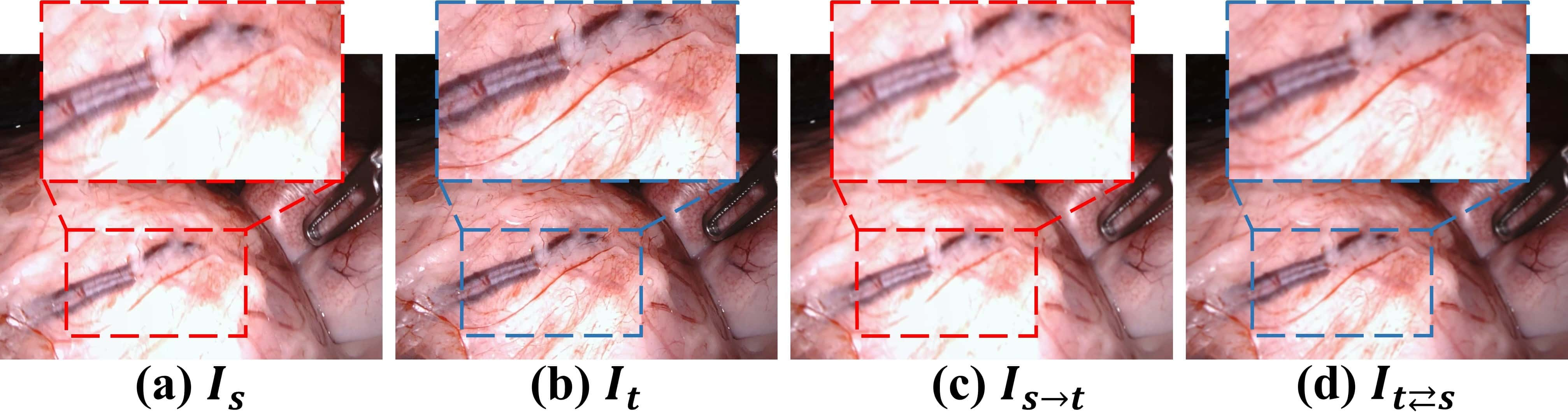
Figure 1: (a)-(b) are the source $I_{s}$ and target $I_{t}$ frames. (c) is the warped image from the source to target. (d) is the cycle-warped image along the target-source-target path for reliable photometric constraint. Box contour colors distinguish different brightness patterns.

The typical solution of monocular depth estimation relies on self-supervised learning, where the core idea is photometric constraint between real and warped images. Specifically, two convolutional neural networks (CNNs) have to be built; one is called DepthNet and the other is PoseNet. The two CNNs estimate a depth map of each image and camera pose changes of every two adjacent images, based on which a source frame in an endoscopic video can be projected into 3D space and warped onto a target view of the other frame. DepthNet and PoseNet are jointly optimized to minimize a photometric loss, which is essentially the pixel-to-pixel difference between the warped and target images.

However, the light source is fixed to the endoscope and moves along with the camera, resulting in significant brightness fluctuations between the source and target frames. Such problem can also be worsened by non-Lambertian reflection due to the close-up observation, as evidenced in Fig. 1(a)-(b). Consequently, between the target and warped source images, the brightness difference dominates as shown in Fig. 1(b)-(c), and thus misguides the photometric constraint in the self-supervised learning.

Many efforts have been paid to enhance the reliability of photometric constraint under the fluctuated brightness. An intuitive solution is to calibrate the brightness in endoscopic video frames beforehand, using either a linear intensity transformation Ozyoruk et al. (2021) or a trained appearance flow model Shao et al. (2022). However, the former only addresses the global brightness inconsistency, and the latter increases the training difficulty due to introduced burdensome computation. Moreover, the reliability of appearance flow model is also not always guaranteed due to the weak self-supervision, which leads to a risk of wrongly modifying areas unrelated to brightness changes.

In this paper, we aim to address the bottleneck of brightness inconsistency without relying on any auxiliary model. Our motivation stems from a recent method named TC-Depth Ruhkamp et al. (2021), which introduced a cycle warping originally for solving the occlusion issue. TC-Depth warps a target image to source and then warps back to itself to identify every occluded pixel, since they assume the occluded pixel can not come back to the original position precisely. We find that such cycle warping can naturally overcome the brightness inconsistency, and yield a more reliable warped image compared to only warping from source to target, as shown in Fig. 1(b)-(d). However, directly applying the cycle warping often fails in photometric constraint because (1) the twice bilinear interpolation of cycle warping blurs the image too much, and (2) the networks of depth&pose estimation are learned actively, which makes the intermediate warping unstable and the convergence difficult.

In view of the above analysis, we propose Monocular depth estimation based on Photometric-invariant Cycle Constraint (MonoPCC), which adopts the idea of cycle warping but significantly reshapes it to enable the photometric constraint invariant to inconsistent brightness. Specifically, MonoPCC starts from the target image, and follows a closed loop path (target-source-target) to obtain a cycle-warped target image, which inherits consistent brightness from the original target image. To make such cycle warping effective in the photometric constraint, MonoPCC employs a learning-free structure transplant module (STM) based on Fast Fourier Transform (FFT) to minimize the negative impact of the blurring effect. STM restores the lost structure details in the intermediate warped image by ‘borrowing’ the phase-frequency part from the source image. Moreover, instead of sharing the network weights in both target-source and source-target warping paths, MonoPCC bridges the two paths using an exponential moving average (EMA) strategy to stabilize the intermediate results in the first path.

In summary, our main contributions are as follows:

1. We propose MonoPCC, which eliminates the inconsistent brightness inducing misguidance in the self-supervised learning by simply adopting a cycle-form warping to render the photometric constraint invariant to the brightness changes.

2. We introduce two enabling techniques, i.e., structure transplant module (STM) and an EMA-based stable training. STM restores the lost image details caused by interpolation, and EMA stabilizes the forward warping. These together guarantee an effective training of MonoPCC under the cycle-form warping.

3. Comprehensive and extensive experimental results on three public datasets demonstrate that MonoPCC outperforms other state-of-the-arts by decreasing the absolute relative error by at least 7.27%, and shows a strong ability to resist inconsistent brightness in the training.

2 Related Work

2.1 Self-Supervised Depth Estimation

Self-supervised methods Zhou et al. (2017); Yin and Shi (2018); Bian et al. (2019); Godard et al. (2019); Watson et al. (2021) of monocular depth estimation mostly, if not all, rely on the photometric constraint to train two networks, named DepthNet and PoseNet. For example, as a pioneering work, SfMLearner Zhou et al. (2017) estimated depth maps and camera poses to synthesize a fake target image by warping another image from the source view, and calculated a reconstruction loss between the warped and target images as the photometric constraint.

For endoscopic cases, M3Depth Huang et al. (2022) enforced not only the photometric constraint but also a 3D geometric structural consistency by Mask-ICP. For improving pose estimation in laparoscopic procedures, Li et al. Li et al. (2022) designed a Siamese pose estimation scheme and also constructed dual-task consistency by additionally predicting scene coordinates. These methods share a common flaw: brightness fluctuations caused by the moving light source in the endoscope, significantly reduce the effectiveness of photometric constraint in self-supervised learning, degrading the performance consequently.

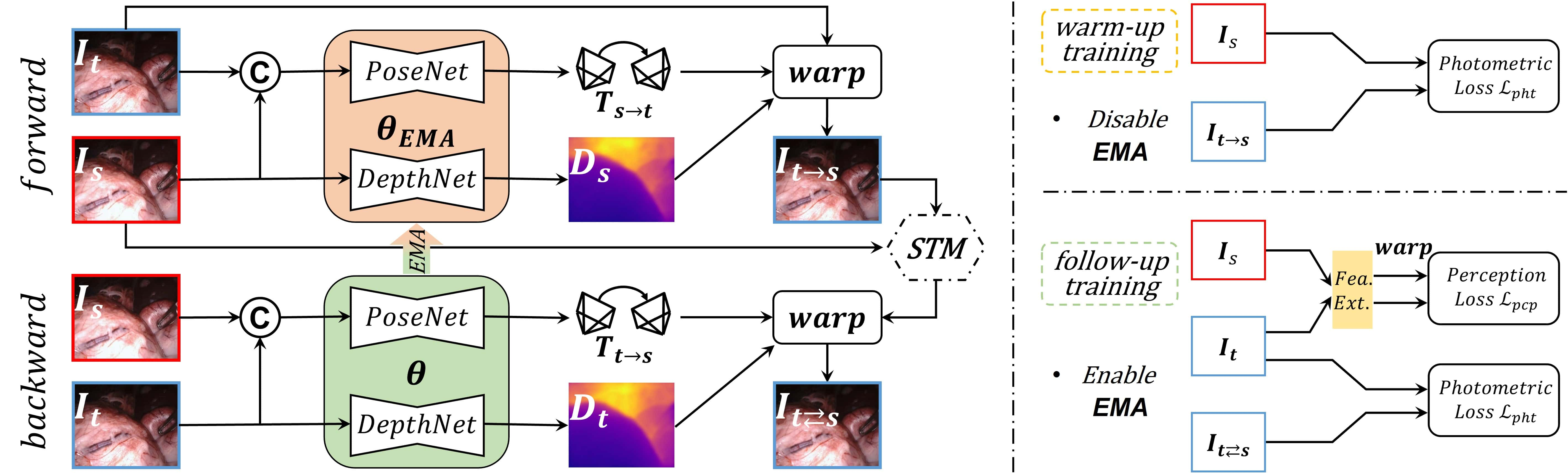
Figure 2: The training pipeline of MonoPCC, which consists of forward and backward cascaded warping paths bridged by two enabling techniques, i.e., structure transplant module (STM) and exponential moving average (EMA). The training has two phases, i.e., warm-up to initialize the network weights for reasonable forward warping, and follow-up to resist the brightness changes. Different box contour colors code different brightness patterns. $\copyright$ means concatenation.

2.2 Brightness Inconsistency

Recently, several efforts have been made to mitigate brightness inconsistency in endoscopic cases, the common solution is to calibrate the brightness inconsistency using either preprocessing or extra learned models. For example, Endo-SfMLearner Ozyoruk et al. (2021) calculated the mean values and standard deviation of images, and then linearly aligned the brightness of the warped image with that of the target one. However, the real brightness fluctuations are actually local and non-linear, and are hardly calibrated by a simple linear transformation. Recently, AF-SfMLearner Shao et al. (2022) tried to relax the requirement of brightness consistency by learning an appearance flow model, which estimates pixel-wise brightness offset between adjacent frames. Nevertheless, effectiveness relies on the quality of the learned appearance flow model, and the risk of wrongly modifying the image content occurs accompanying the model error. Also, introducing an extra model dramatically increases the training time and difficulty in self-supervised learning.

3 Method

Fig. 2 illustrates the pipeline of MonoPCC, consisting of both forward and backward warping paths in the training phase. We first explain how to warp images for self-supervised learning in Sec. 3.1, and then detail the photometric-invariant principle of MonoPCC in Sec. 3.2, as well as its two key enabling techniques in Sec. 3.3 and Sec. 3.4, i.e., structure transplant module (STM) for avoiding detail lost and EMA between two paths for stabilizing the training.

3.1 Warping across Views for Self-Supervision

To warp a source image $I_{s}$ to a target view $I_{t}$, DepthNet and PoseNet first estimate the target depth map $D_{t}$, and the camera pose changing from target to source $T_{t\rightarrow s}$, respectively.

The DepthNet is typically an encoder-decoder, which inputs a single endoscopic image and outputs an aligned depth map. In this work, we use MonoViT Zhao et al. (2022) as our backbone DepthNet. The PoseNet contains a lightweight ResNet18-based He et al. (2016) encoder with four convolutional layers, which inputs a concatenated two images and predicts the pose change from the image in the tail channels to that in the front channels.

Using $D_{t}$ and $T_{t\rightarrow s}$, the warping can be performed from the source to target view, and each pixel in the warped image $I_{s\rightarrow t}$ can find its matching pixel in the source image using the following equation:

$$p_{s}=KT_{t\rightarrow s}D_{t}(p_{s\rightarrow t})K^{-1}p_{s\rightarrow t},$$ (1)

where $p_{s}$ and $p_{s\rightarrow t}$ are the pixel’s homogeneous coordinates in $I_{s}$ and $I_{s\rightarrow t}$, respectively, $D(p)$ means the depth value of $D$ at the position $p$, and $K$ denotes the given camera intrinsic matrix. With the pixel matching relationship, $I_{s\rightarrow t}$ can be obtained by filling the color at each pixel position using differentiable bilinear sampling Jaderberg et al. (2015):

$$I_{s\rightarrow t}(p_{s\rightarrow t})=\mathtt{BilinearSampler}(I_{s}(p_{s})),$$ (2)

where $I(p)$ means the pixel intensity of $I$ at the position $p$. Since $p_{s\rightarrow t}$ is discrete and $p_{s}$ is continuous, $\mathtt{BilinearSampler}$ is utilized to calculate the intensity of each pixel in $I_{s\rightarrow t}$ using the neighboring pixels around $p_{s}$ and allow error backpropagation.

After warping, DepthNet and PoseNet can be constrained via the photometric loss, which is calculated as follows:

$$\begin{split}\mathcal{L}_{pht}(I_{t},I_{s\rightarrow t})&=\alpha\cdot\frac{1-\operatorname{SSIM}(I_{t},I_{s\rightarrow t})}{2}\\ &+(1-\alpha)\cdot|I_{t}-I_{s\rightarrow t}|,\end{split}$$ (3)

where Structure Similarity Index Measure (SSIM) Wang et al. (2004) constrains the image quality and L1 loss constrains the content. $\alpha$ is set to 0.85 according to Godard et al. (2017).

One of the assumptions for the photometric constraint in Eq. (3) is that the scene contains no specular reflections, and is temporally consistent in terms of brightness Shao et al. (2022). However, such assumption hardly holds true in the endoscopic cases as visualized in Fig. 1.

3.2 Photometric-invariant Cycle Warping

To overcome the brightness inconsistency, we construct a cycle loop path involving forward and backword warping, as shown in Fig. 2. To better explain the principle, we use the red and blue box contours to indicate the different brightness patterns carried by the image.

To get a warped image inheriting the target’s brightness, we start from the target itself, and first warp it to get $I_{t\rightarrow s}$, and then warp back to get $I_{t\rightleftarrows s}$. The pixel matching relationships across the three images are formulated as follows:

$$\left\downarrow\begin{aligned} &p_{t}=KT_{s\rightarrow t}D_{s}(p_{t\rightarrow s})K^{-1}p_{t\rightarrow s},\\ &p_{t\rightarrow s}=KT_{t\rightarrow s}D_{t}(p_{t\rightleftarrows s})K^{-1}p_{t\rightleftarrows s},\end{aligned}\right.$$ (4)

where $p_{t}$, $p_{t\rightarrow s}$, and $p_{t\rightleftarrows s}$ are the pixel’s homogeneous coordinates in $I_{t}$, $I_{t\rightarrow s}$ and $I_{t\rightleftarrows s}$, respectively. $D_{s}$ and $D_{t}$ are DepthNet-predicted depth maps of the source and target images, respectively.

Therefore, according to Eq. (2), $I_{t\rightarrow s}$ and $I_{t\rightleftarrows s}$ can be obtained sequentially:

$$\left\downarrow\begin{aligned} &I_{t\rightarrow s}(p_{t\rightarrow s})=\mathtt{BilinearSampler}(I_{t}(p_{t})),\\ &I_{t\rightleftarrows s}(p_{t\rightleftarrows s})=\mathtt{BilinearSampler}(I_{t\rightarrow s}(p_{t\rightarrow s})).\end{aligned}\right.$$ (5)

Thus, we rewrite the previous photometric constraint Eq. (3) to a cycle form, i.e., $\mathcal{L}_{pht}(I_{t},I_{t\rightleftarrows s})$, where $I_{t}$ and $I_{t\rightleftarrows s}$ have the same brightness pattern as shown in Fig. 2. However, direct usage of such cycle warping brings two issues in the optimization of photometric constraint: (1) noticeable image detail lost due to twice image interpolation using $\mathtt{BilinearSampler}$, which negatively affects the appearance-based photometric constraint, and (2) the networks learn too actively to give stable intermediate warping, making the training of two networks difficult to converge. Thus, we introduce two enabling techniques, i.e., structure transplant module to retain structure details and EMA strategy to stabilize forward warping.

3.3 Structure Transplant to Retain Details

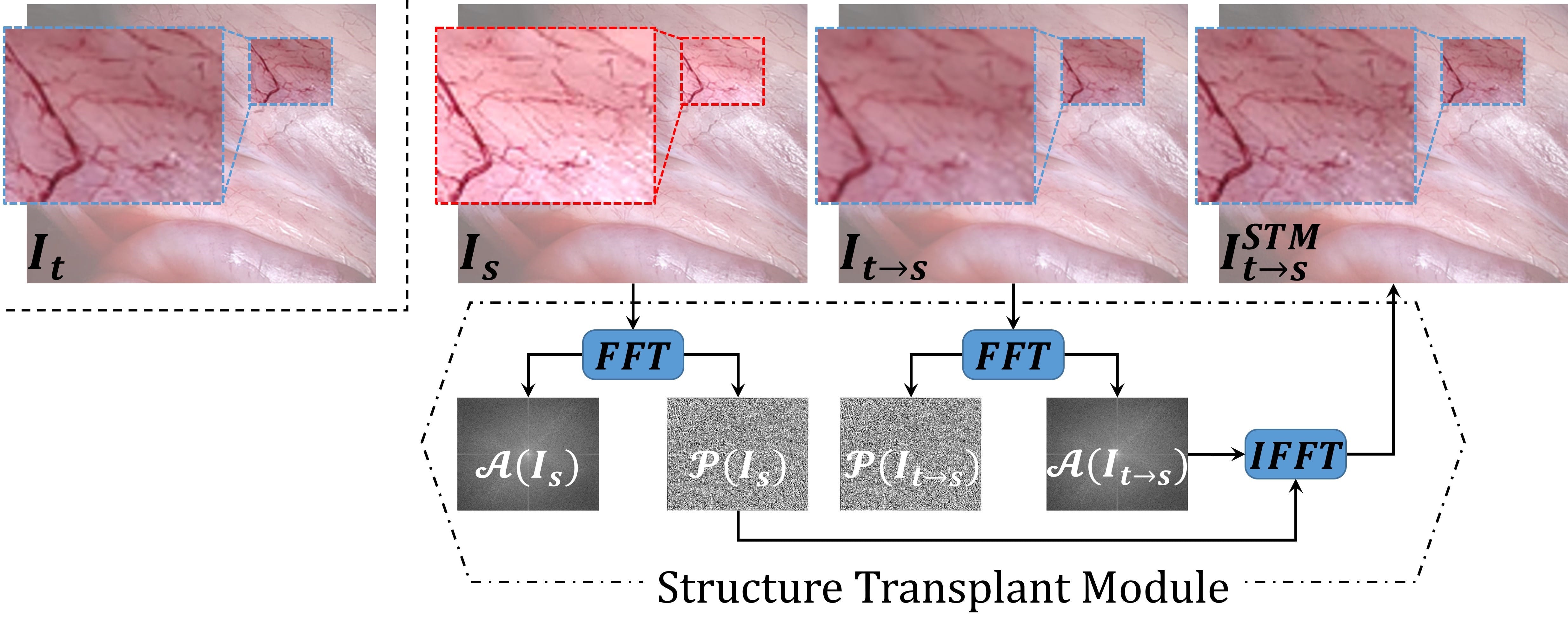
Figure 3: Details of STM, which utilizes the phase-frequency of the source image $I_{s}$ to replace that of the warped image $I_{t\rightarrow s}$ to avoid image detail lost.

The learning-free structure transplant module (STM) works based on two observations: (1) the warped frame $I_{t\rightarrow s}$ has homologous image style as $I_{t}$, and (2) the original frame $I_{s}$ has real structure details, and also is roughly aligned with $I_{t\rightarrow s}$. Inspired by the image-aligned style transformation proposed in Lv et al. (2023), we transplant fine structure of $I_{s}$ onto the appearance of $I_{t\rightarrow s}$ via a learning-free style transformation approach illustrated in Fig. 3.

Specifically, STM utilizes Fast Fourier Transform (FFT) Nussbaumer and Nussbaumer (1982) to decompose an RGB image $x$ into two components, i.e., amplitude $\mathcal{A}(x)$ and phase $\mathcal{P}(x)$. $\mathcal{A}(x)$ mainly controls the image style like brightness and $\mathcal{P}(x)$ contains the information of structure details Lv et al. (2023). Thus, after the forward warping, STM recombines $\mathcal{A}(I_{t\rightarrow s})$ and $\mathcal{P}(I_{s})$, and produces the structure-restored warped image $I_{t\rightarrow s}^{STM}$ via Inverse Fast Fourier Transform (IFFT):

$$I_{t\rightarrow s}^{STM}=IFFT(\mathcal{A}(I_{t\rightarrow s})*e^{-j*\mathcal{P}(I_{s})}).$$ (6)

Therefore, in the backward warping, we utilize $I_{t\rightarrow s}^{STM}$ to substitute $I_{t\rightarrow s}$ in Eq. (5), which can be rewritten as follows:

$$I_{t\rightleftarrows s}(p_{t\rightleftarrows s})=\mathtt{BilinearSampler}(I_{t\rightarrow s}^{STM}(p_{t\rightarrow s})).$$ (7)

As shown in Fig. 3, $I_{t\rightarrow s}^{STM}$ displays better structure details than $I_{t\rightarrow s}$, and also maintains similar illumination as $I_{t\rightarrow s}$.

3.4 EMA to Stabilize Forward Warping

As shown in Fig. 2, the two paths are connected in a cascaded fashion, where the result of the second warping relies on the output of the previous warping. Therefore, a well-initialized and steady intermediate warped image $I_{t\rightarrow s}$ is very important for a stable convergence of training. In view of this, we introduce an exponential moving average (EMA) to bridge the two paths and thus divide the whole training into warm-up and follow-up phases.

During the warm-up training, EMA is disabled and we only train DepthNet and PoseNet in the forward warping by optimizing the photometric constraint between $I_{s}$ and $I_{t\rightarrow s}$, that is, $\theta=\arg\min_{\theta}\mathcal{L}_{pht}(I_{s},I_{t\rightarrow s})$, where $\theta$ represents the total learnable parameters of both DepthNet and PoseNet. Although the brightness inconsistency occurs in the warm-up training, a reasonably acceptable initialization of DepthNet and PoseNet can be reached.

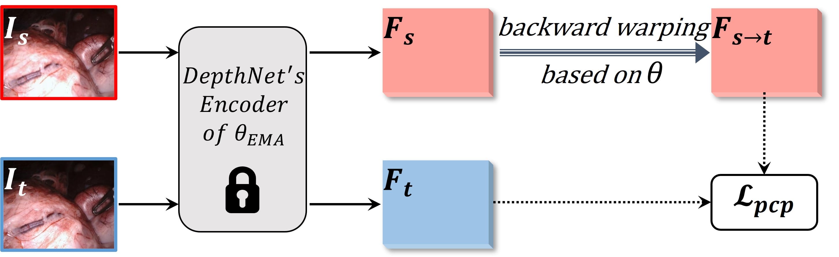
Figure 4: The auxiliary perception constraint by backward warping the encoding feature maps instead of raw images.

The follow-up training with EMA enabled is the key step to resist brightness inconsistency based on the cycle warping. We duplicate the network parameters learned in the warm-up training as an EMA copy $\theta_{EMA}\leftarrow\theta$, and use the models with $\theta_{EMA}$ to estimate depth and pose in the forward warping and those with $\theta$ in the backward warping. $\theta$ is updated actively by minimizing the cycle-form photometric loss $L_{pht}(I_{t},I_{t\rightleftarrows s})$, and $\theta_{EMA}$ is updated slowly by moving averaging $\theta$. That is, the copy of DepthNet and PoseNet for the forward warping is not directly learned by the optimization of photometric constraint in the follow-up training, thus to avoid predicting frequently changed $I_{t\rightarrow s}$.

Besides, we further enhance the learning robustness via a ready-made perception loss. As shown in Fig. 4, we backward warp the encoding map of $I_{s}$ generated from DepthNet’s encoder of its EMA version, yielding a warped feature map $F_{s\rightarrow t}$. If we also extract the encoding map of $I_{t}$ using the same encoder, $F_{s\rightarrow t}$ and $F_{t}$ should be aligned and may contain high-level semantic information covering the low-level brightness changes. Thus, a perception loss is defined:

$$\mathcal{L}_{pcp}(F_{t},F_{s\rightarrow t})=|F_{t}-F_{s\rightarrow t}|.$$ (8)

In summary, the follow-up training of MonoPCC is formulated as follows:

$$\left\{\begin{aligned} &\theta=\arg\min_{\theta}(\mathcal{L}_{pht}(I_{t},I_{t\rightleftarrows s})+\mathcal{L}_{pcp}(F_{t},F_{s\rightarrow t})),\\ &\theta_{EMA}=\alpha\theta_{EMA}+(1-\alpha)\theta,\end{aligned}\right.$$ (9)

where $\alpha$ is a hyperparameter to balance the stability and learnability of the forward warping, and set to $0.75$ in MonoPCC by default.

3.5 Implementation Details

We train MonoPCC using a single NVIDIA RTX A6000 GPU. We utilize MonoViT and ResNet18 pre-trained on ImageNetDeng et al. (2009) for DepthNet and PoseNet initialization, respectively. We set the batch size to 12, and use AdamW Loshchilov and Hutter (2017) as the optimizer. The learning rate decay is exponential and set to 0.9. The number of epochs and learning rate differ in the warm-up and follow-up training phases. In warm-up training, the number of epochs is set to 20 epochs, and the initial learning rate is set to $1\times 10^{-4}$ for DepthNet’s encoder and $5\times 10^{-5}$ for the rest weights. In follow-up training, the number of epochs is set to 10 epochs, and the initial learning rate is set to $5\times 10^{-5}$ for all network weights.

4 Experimental Settings

4.1 Comparison Methods

We compare MonoPCC with 8 state-of-the-art (SOTA) methods of monocular depth estimation, i.e., Monodepth2 Godard et al. (2019), FeatDepth Shu et al. (2020), HR-Depth Lyu et al. (2021), DIFFNet Zhou et al. (2021), Endo-SfMLearner Ozyoruk et al. (2021), AF-SfMLearner Shao et al. (2022), MonoViT Zhao et al. (2022), and Lite-Mono Zhang et al. (2023). We evaluate their performance and make comparisons using their released codes.

4.2 Datasets

The experiment in this work involves 3 public endoscopic datasets, i.e., SCARED Allan et al. (2021), SimCol3D Rau et al. (2023), and SERV-CT Edwards et al. (2022).

SCARED is from a MICCAI challenge and consists of 35 videos with the size of $1280\times 1024$ collected from porcine cadavers using a da Vinci Xi surgical robot. Structured light is used to obtain the ground-truth (GT) depth map for the first frame, which is then mapped onto the subsequent frames using camera trajectory recorded by the robotic arm.

Since the original data is binocular, we only use the left view to simulate our focusing monocular situation. We split the dataset into 21,066 frames for training and 551 for test, which are consistent with the previous SOTA Shao et al. (2022). No videos are cross-used in both training and test.

SimCol3D is from MICCAI 2022 EndoVis challenge. It is a synthetic dataset which contains over 36,000 colonoscopic images and depth annotations with size of $475\times 475$. Meanwhile, virtual light sources are attached to the camera. For the usage of SimCol3D dataset, we follow their official website and spilt the dataset into 28,776 and 9,009 frames for training and test, respectively.

SERV-CT is collected from two ex vivo porcine cadavers, and each has 8 binocular keyframes. We treat the two views independently and thus have 32 images in total with the size of $720\times 576$. The GT depth map for each image is calculated by manually aligning the endoscopic image to the 3D anatomical model derived from the corresponding CT scan.

Metric	Formula
Abs Rel	$\frac{1}{N}{\sum\limits_{i=0}^{N-1}{|d_{i}-d_{i}^{*}|}/{d_{i}^{*}}}$
Sq Rel	$\frac{1}{N}{\sum\limits_{i=0}^{N-1}{|d_{i}-d_{i}^{*}|^{2}}/{d_{i}^{*}}}$
RMSE	$\sqrt{\frac{1}{N}{\sum\limits_{i=0}^{N-1}{|d_{i}-d_{i}^{*}|}^{2}}}$
RMSE log	$\sqrt{\frac{1}{N}{\sum\limits_{i=0}^{N-1}{|log\,d_{i}-log\,d_{i}^{*}|}^{2}}}$
$\delta$	$\frac{1}{N}\sum\limits_{i=0}^{N-1}[max(\frac{d_{i}}{d_{i}^{*}},\frac{d_{i}^{*}}{d_{i}})\,<\,1.25]$

Table 1: Evaluation metrics of monocular depth estimation, where $N$ refers to the number of valid pixels in depth maps, $d_{i}$ and $d_{i}^{*}$ denote the estimated and GT depth of $i$-th pixel, respectively. The Iverson bracket $[\cdot]$ yields 1 if the statement is true, otherwise 0.

Methods	SCARED					SimCol3D
	Abs Rel $\downarrow$	Sq Rel $\downarrow$	RMSE $\downarrow$	RMSE log $\downarrow$	$\delta$ $\uparrow$	Abs Rel $\downarrow$	Sq Rel $\downarrow$	RMSE $\downarrow$	RMSE log $\downarrow$	$\delta$ $\uparrow$
Monodepth2	0.060	0.432	4.885	0.082	0.972	0.076	0.061	0.402	0.106	0.950
FeatDepth	0.055	0.392	4.702	0.077	0.976	0.077	0.069	0.374	0.098	0.957
HR-Depth	0.058	0.439	4.886	0.081	0.969	0.072	0.044	0.378	0.100	0.961
DIFFNet	0.057	0.423	4.812	0.079	0.975	0.074	0.053	0.401	0.105	0.957
Endo-SfMLearner	0.057	0.414	4.756	0.078	0.976	0.072	0.042	0.407	0.103	0.950
AF-SfMLearner	0.055	0.384	4.585	0.075	0.979	0.071	0.045	0.372	0.099	0.961
MonoViT	0.057	0.416	4.919	0.079	0.977	0.064	0.034	0.377	0.094	0.968
Lite-Mono	0.056	0.398	4.614	0.077	0.974	0.076	0.050	0.424	0.110	0.950
MonoPCC(Ours)	0.051	0.349	4.488	0.072	0.983	0.058	0.028	0.347	0.090	0.975

Table 2: Quantitative comparison results on SCARED and SimCol3D. The best results are marked in bold and the second-best underlined. The paired p-values between MonoPCC and others are all less than $0.05$.

Figure 5: The Abs Rel error maps of comparison methods on the three datasets. Opencv Jet Colormap is used for visualization.

4.3 Evaluation Metrics

To be consistent with previous works, we employ 5 metrics in the evaluation, which are listed in Table 1. Note that, as the common evaluation routine of monocular depth estimation, the predicted depth map should be scaled beforehand since it is scale unknown. The scaling factor is the GT median depth divided by the predicted median depth Zhou et al. (2017).

5 Results and Discussions

5.1 Comparison with State-of-the-arts

5.1.1 Evaluation on SCARED and SimCol3D

Table 2 shows the comparison results on SCARED (left part) and SimCol3D (right part). As can be seen, our method achieves the best performance in terms of all five metrics on SCARED, and consistently outperforms the other SOTAs by different margins on SimCol3D.

Likewise, Endo-SfMLearner and AF-SfMLearner also belong to the approach of addressing the brightness inconsistency in self-supervised monocular depth estimation. Endo-SfMLearner adopts the simple idea of brightness linear transformation, while AF-SfMLearner resorts to a more complex appearance flow model. From their results, we can see that the appearance flow model is more effective, since the brightness changes are often non-linear in the endoscopic scene. Nevertheless, our MonoPCC still exceeds the AF-SfMLearner by reducing Sq Rel by 9.11% on SCARED, which implies that compared to the learning-based appearance flow model, our cycle-form warping can guarantee the brightness consistency in a more effective and reliable way.

The top four rows of Fig. 5 present a qualitative comparison on the two datasets. Error maps are acquired by mapping pixel-wise Abs Rel value to different colors, and the red means large relative error and the blue indicates small error. On SCARED, the color-coded error map of MonoPCC is clearly bluer than those of other SOTAs, especially for the regions near the boundaries or specular reflections, as indicated by the red dotted boxes in Fig. 5.

On SimCol3D, MonoPCC provides lower relative depth errors at both the proximal and distal parts of the colon, which demonstrates the validity of MonoPCC for low-textured regions, e.g., colon in the digestive tract.

Methods	Abs Rel $\downarrow$	Sq Rel $\downarrow$	RMSE $\downarrow$	RMSE log $\downarrow$	$\delta$ $\uparrow$
Monodepth2	0.127	2.152	13.023	0.166	0.825
FeatDepth	0.117	1.862	12.040	0.154	0.841
HR-Depth	0.122	2.085	12.587	0.156	0.850
DIFFNet	0.116	1.858	12.177	0.146	0.864
Endo-SfMLearner	0.122	2.123	12.551	0.168	0.842
AF-SfMLearner	0.101	1.546	10.900	0.131	0.888
MonoViT	0.103	1.566	11.482	0.136	0.895
Lite-Mono	0.124	2.314	13.156	0.175	0.820
MonoPCC(Ours)	0.091	1.252	10.059	0.116	0.915

Table 3: Quantitative comparison results on SERV-CT. The best results are marked in bold and the second-best underlined. The paired p-values between MonoPCC and others are all less than $0.05$, except for $\delta$ compared to MonoViT.

5.1.2 Generalization on SERV-CT

We also evaluate the generalization of all methods, i.e., using the model trained on SCARED to directly test on SERV-CT. The comparison results are listed in Table 3. As can be seen, all methods experience a varying degree of degradation on SERV-CT. However, MonoPCC is still the best, and the only one maintaining the Abs Rel less than $0.1$ and $\delta$ greater than $0.9$. Also, MonoPCC significantly surpasses the second-best AF-SfMLearner by a relative decrease of 19.02% and 11.45% in the Sq Rel and RMSE log, respectively. The bottom two rows of Fig. 5 exhibit two visual results from SERV-CT. As can be seen, most methods yield higher errors compared to their visual results on SCARED. In comparison, MonoPCC still produces less red error maps as indicated by the dotted boxes in Fig. 5.

5.2 Ablation Study

We conduct ablation studies via 5-fold cross-validation on SCARED to verify the effectiveness of each component in MonoPCC and to compare MonoPCC with other related techniques against brightness fluctuations.

Cycle	STM	EMA	$\mathcal{L}_{pcp}$	Abs Rel $\downarrow$	Sq Rel $\downarrow$	RMSE $\downarrow$	RMSE log $\downarrow$
$\Circle$	✗	✗	✗	0.106$\pm$0.051	1.533$\pm$1.383	9.737$\pm$5.221	0.141$\pm$0.060
$\CIRCLE$	✗	✗	✗	0.110$\pm$0.047	1.584$\pm$1.315	10.003$\pm$4.930	0.145$\pm$0.056
$\CIRCLE$	✗	✓	✓	0.108$\pm$0.048	1.596$\pm$1.329	10.047$\pm$5.335	0.144$\pm$0.060
$\CIRCLE$	✓	✗	✗	0.099$\pm$0.043	1.286$\pm$1.091	9.007$\pm$4.697	0.131$\pm$0.052
$\CIRCLE$	✓	✗	✓	0.091$\pm$0.031	1.040$\pm$0.700	8.239$\pm$3.664	0.120$\pm$0.041
$\CIRCLE$	✓	✓	✗	0.091$\pm$0.036	1.081$\pm$0.800	8.355$\pm$3.905	0.121$\pm$0.045
$\CIRCLE$	✓	✓	✓	0.085$\pm$0.034	0.953$\pm$0.712	7.734$\pm$3.537	0.114$\pm$0.044

Table 4: The rows except the first one are the comparison results of the five variants and the complete MonoPCC, which are all cycle-constrained. The first row is the backbone MonoViT using the regular non-cycle constraint.

5.2.1 Effectiveness of Three Components

We develop five variants of MonoPCC by disabling the three components, EMA and/or $\mathcal{L}_{pcp}$, and STM. Note that, the warping should be cycle-form to utilize the components, and if we disable EMA, only $\theta$ in the backward warping path will be updated, and $\theta_{EMA}$ in the forward warping remains unchanged. Table 4 gives the comparison results between the variants and complete MonoPCC. We also include the backbone MonoViT in the first row of Table 4 as the baseline, which adopts the non-cycle warping.

From the comparison results in Table 4, three key observations can be made:

(1) By comparing the first two rows of Table 4, the inferior performance of the variant using none of the components indicates that the direct usage of cycle warping is not enough due to the image blurring and unstable gradient propagation mentioned in Sec. 3.2.

(2) As can be seen from the second to fourth rows, using EMA and $\mathcal{L}_{pcp}$ solely brings no improvements. However, adding STM can significantly reduce Sq Rel and RMSE by 16.11% and 7.50%, respectively ($p<0.003$). Thus, STM is the irreplaceable component for successfully training using the cycle-form warping.

(3) Comparison between the last four rows reveals the effectiveness of EMA and $\mathcal{L}_{pcp}$. Specifically, with STM enabled, both EMA and $\mathcal{L}_{pcp}$ bring remarkable reduction of Abs Rel by 8.08% ($p=0.012$, $p=0.022$). Meanwhile, EMA and $\mathcal{L}_{pcp}$ are not mutually excluded, and the combination reduces Abs Rel by 14.14% ($p=0.001$).

Schemes	Abs Rel $\downarrow$	Sq Rel $\downarrow$	RMSE $\downarrow$	RMSE log $\downarrow$
Baseline	0.106$\pm$0.051	1.533$\pm$1.383	9.737$\pm$5.221	0.141$\pm$0.060
ABT	0.102$\pm$0.046	1.425$\pm$1.214	9.366$\pm$4.784	0.137$\pm$0.056
AFM	0.098$\pm$0.039	1.251$\pm$0.964	8.897$\pm$4.203	0.130$\pm$0.049
STM+EMA	0.091$\pm$0.036	1.081$\pm$0.800	8.355$\pm$3.905	0.121$\pm$0.045

Table 5: Comparison results of different techniques for addressing the brightness fluctuations in self-supervised learning. The last row is the technique used in MonoPCC.

Figure 6: An example of created brightness perturbation. From left to right is the original image, globally perturbated ($k=1.2$), and both globally and locally (bright spots) perturbated. The color-coded maps above them describe the subtractive difference between the perturbated image and its original one.

5.2.2 MonoPCC vs. Other Techniques against Brightness Fluctuations

Several techniques have been developed to address inconsistent brightness in endoscopic images, e.g., affine brightness transformation (ABT) in Endo-SfMLearner, and appearance flow module (AFM) in AF-SfMLearner. For comparison, we train three variants of the backbone MonoViT, using ABT, AFM, and STM+EMA, respectively, to verify the robustness of different enabling techniques to the brightness inconsistency.

Table 5 lists the comparison results as well as the backbone MonoViT using none of these techniques. As can be seen, the variant using STM+EMA strategy exceeds that using AFM only with a reduction of Abs Rel and Sq Rel by 7.14% and 13.59%, respectively ($p=0.019$, $p=0.014$). It is worth noting that compared to AFM, our method requires no extra model to learn, exhibiting greater usability and scalability.

5.3 Robustness to Severe Brightness Inconsistency

Besides the current inconsistent brightness carried by the used dataset, we want to test the limit of MonoPCC under more severe brightness fluctuations. To this end, we create two copies of SCARED, and add global brightness perturbation to every adjacent frames of the first copy, and both global and local perturbations to the second. Specifically, the global perturbation is defined as the linear transformation on the image’s brightness channel (HSV color model), that is, $v^{scale}=k*v,k\in[0.8,0.9]\cup[1.1,1.2]$. The local perturbation is the randomly placed Gaussian bright (or dark) spots. Fig. 6 presents visual examples from the original SCARED and our created two copies with more severe brightness inconsistency.

Figure 7: The Abs Rel errors of different methods trained on the two brightness-perturbed copies of SCARED and the original SCARED.

Fig. 7 illustrates Abs Rel errors of different methods on the two brightness-perturbed copies of and the original SCARED. As mentioned before, Endo-SfMLearner and AF-SfMLearner all tried to address the brightness inconsistency. As can be seen from the comparison results, Endo-SfMLearner shows a robustness to the global brightness perturbation thanks to its using brightness linear transformation, but degrades significantly when facing the local perturbation. AF-SfMLearner can address the local brightness perturbation more or less using a learned appearance flow model, but still presents a non-trivial increase of Abs Rel error. In comparison, MonoPCC achieves the lowest Abs Rel error on the three datasets, and even produces lower errors on the copy containing the most severe brightness inconsistency (global+local) compared to the other methods’ results on the original SCARED.

6 Conclusion

Self-supervised monocular depth estimation is challenging for endoscopic scenes due to the severe negative impact of brightness fluctuations on the photometric constraint. In this paper, we propose a cycle-form warping to naturally overcome the brightness inconsistency of endoscopic images, and develop a MonoPCC for robust monocular depth estimation by using a re-designed photometric-invariant cycle constraint. To make the cycle-form warping effective in the photometric constraint, MonoPCC is equipped with two enabling techniques, i.e., structure transplant module (STM) and exponential moving average (EMA) strategy. STM alleviates image detail degradation to validate the backward warping, which uses the result of forward warping as input. EMA bridges the learning of network weights in the forward and backward warping, and stabilizes the intermediate warped image to ensure an effective convergence. The comprehensive and extensive comparisons with $8$ state-of-the-arts on three public datasets, i.e., SCARED, SimCol3D, and SERV-CT, demonstrate that MonoPCC achieves a superior performance by decreasing the absolute relative error by at least $7.27\%$. Additionally, two ablation studies are conducted to confirm the effectiveness of three developed modules and the advancement of MonoPCC over other similar techniques against brightness fluctuations. In the future work, we plan to extend MonoPCC into the multi-frame based monocular depth estimation.

References

- Allan et al. [2021] Max Allan, Jonathan Mcleod, Congcong Wang, Jean Claude Rosenthal, Zhenglei Hu, Niklas Gard, Peter Eisert, Ke Xue Fu, Trevor Zeffiro, Wenyao Xia, et al. Stereo correspondence and reconstruction of endoscopic data challenge. arXiv preprint arXiv:2101.01133, 2021.
- Bian et al. [2019] Jiawang Bian, Zhichao Li, Naiyan Wang, Huangying Zhan, Chunhua Shen, Ming-Ming Cheng, and Ian Reid. Unsupervised scale-consistent depth and ego-motion learning from monocular video. Advances in neural information processing systems, 32, 2019.
- Deng et al. [2009] Jia Deng, Wei Dong, Richard Socher, Li-Jia Li, Kai Li, and Li Fei-Fei. Imagenet: A large-scale hierarchical image database. In 2009 IEEE conference on computer vision and pattern recognition, pages 248–255. Ieee, 2009.
- Edwards et al. [2022] PJ Eddie Edwards, Dimitris Psychogyios, Stefanie Speidel, Lena Maier-Hein, and Danail Stoyanov. Serv-ct: A disparity dataset from cone-beam ct for validation of endoscopic 3d reconstruction. Medical image analysis, 76:102302, 2022.
- Godard et al. [2017] Clément Godard, Oisin Mac Aodha, and Gabriel J Brostow. Unsupervised monocular depth estimation with left-right consistency. In Proceedings of the IEEE conference on computer vision and pattern recognition, pages 270–279, 2017.
- Godard et al. [2019] Clément Godard, Oisin Mac Aodha, Michael Firman, and Gabriel J Brostow. Digging into self-supervised monocular depth estimation. In Proceedings of the IEEE/CVF international conference on computer vision, pages 3828–3838, 2019.
- He et al. [2016] Kaiming He, Xiangyu Zhang, Shaoqing Ren, and Jian Sun. Deep residual learning for image recognition. In Proceedings of the IEEE conference on computer vision and pattern recognition, pages 770–778, 2016.
- Huang et al. [2022] Baoru Huang, Jian-Qing Zheng, Anh Nguyen, Chi Xu, Ioannis Gkouzionis, Kunal Vyas, David Tuch, Stamatia Giannarou, and Daniel S Elson. Self-supervised depth estimation in laparoscopic image using 3d geometric consistency. In International Conference on Medical Image Computing and Computer-Assisted Intervention, pages 13–22. Springer, 2022.
- Jaderberg et al. [2015] Max Jaderberg, Karen Simonyan, Andrew Zisserman, et al. Spatial transformer networks. Advances in neural information processing systems, 28, 2015.
- Li et al. [2022] Wenda Li, Yuichiro Hayashi, Masahiro Oda, Takayuki Kitasaka, Kazunari Misawa, and Kensaku Mori. Geometric constraints for self-supervised monocular depth estimation on laparoscopic images with dual-task consistency. In International Conference on Medical Image Computing and Computer-Assisted Intervention, pages 467–477. Springer, 2022.
- Loshchilov and Hutter [2017] Ilya Loshchilov and Frank Hutter. Decoupled weight decay regularization. arXiv preprint arXiv:1711.05101, 2017.
- Lv et al. [2023] Jinxin Lv, Xiaoyu Zeng, Sheng Wang, Ran Duan, Zhiwei Wang, and Qiang Li. Robust one-shot segmentation of brain tissues via image-aligned style transformation. In Proceedings of the AAAI Conference on Artificial Intelligence, volume 37, pages 1861–1869, 2023.
- Lyu et al. [2021] Xiaoyang Lyu, Liang Liu, Mengmeng Wang, Xin Kong, Lina Liu, Yong Liu, Xinxin Chen, and Yi Yuan. Hr-depth: High resolution self-supervised monocular depth estimation. In Proceedings of the AAAI Conference on Artificial Intelligence, volume 35, pages 2294–2301, 2021.
- Nussbaumer and Nussbaumer [1982] Henri J Nussbaumer and Henri J Nussbaumer. The fast Fourier transform. Springer, 1982.
- Ozyoruk et al. [2021] Kutsev Bengisu Ozyoruk, Guliz Irem Gokceler, Taylor L Bobrow, Gulfize Coskun, Kagan Incetan, Yasin Almalioglu, Faisal Mahmood, Eva Curto, Luis Perdigoto, Marina Oliveira, et al. Endoslam dataset and an unsupervised monocular visual odometry and depth estimation approach for endoscopic videos. Medical image analysis, 71:102058, 2021.
- Rau et al. [2023] Anita Rau, Binod Bhattarai, Lourdes Agapito, and Danail Stoyanov. Bimodal camera pose prediction for endoscopy. IEEE Transactions on Medical Robotics and Bionics, 2023.
- Ruhkamp et al. [2021] Patrick Ruhkamp, Daoyi Gao, Hanzhi Chen, Nassir Navab, and Beniamin Busam. Attention meets geometry: Geometry guided spatial-temporal attention for consistent self-supervised monocular depth estimation. In 2021 International Conference on 3D Vision (3DV), pages 837–847. IEEE, 2021.
- Shao et al. [2022] Shuwei Shao, Zhongcai Pei, Weihai Chen, Wentao Zhu, Xingming Wu, Dianmin Sun, and Baochang Zhang. Self-supervised monocular depth and ego-motion estimation in endoscopy: Appearance flow to the rescue. Medical image analysis, 77:102338, 2022.
- Shu et al. [2020] Chang Shu, Kun Yu, Zhixiang Duan, and Kuiyuan Yang. Feature-metric loss for self-supervised learning of depth and egomotion. In European Conference on Computer Vision, pages 572–588. Springer, 2020.
- Wang et al. [2004] Zhou Wang, Alan C Bovik, Hamid R Sheikh, and Eero P Simoncelli. Image quality assessment: from error visibility to structural similarity. IEEE transactions on image processing, 13(4):600–612, 2004.
- Watson et al. [2021] Jamie Watson, Oisin Mac Aodha, Victor Prisacariu, Gabriel Brostow, and Michael Firman. The temporal opportunist: Self-supervised multi-frame monocular depth. In Proceedings of the IEEE/CVF Conference on Computer Vision and Pattern Recognition, pages 1164–1174, 2021.
- Yin and Shi [2018] Zhichao Yin and Jianping Shi. Geonet: Unsupervised learning of dense depth, optical flow and camera pose. In Proceedings of the IEEE conference on computer vision and pattern recognition, pages 1983–1992, 2018.
- Zhang et al. [2023] Ning Zhang, Francesco Nex, George Vosselman, and Norman Kerle. Lite-mono: A lightweight cnn and transformer architecture for self-supervised monocular depth estimation. In Proceedings of the IEEE/CVF Conference on Computer Vision and Pattern Recognition, pages 18537–18546, 2023.
- Zhao et al. [2022] Chaoqiang Zhao, Youmin Zhang, Matteo Poggi, Fabio Tosi, Xianda Guo, Zheng Zhu, Guan Huang, Yang Tang, and Stefano Mattoccia. Monovit: Self-supervised monocular depth estimation with a vision transformer. In 2022 International Conference on 3D Vision (3DV), pages 668–678. IEEE, 2022.
- Zhou et al. [2017] Tinghui Zhou, Matthew Brown, Noah Snavely, and David G Lowe. Unsupervised learning of depth and ego-motion from video. In Proceedings of the IEEE conference on computer vision and pattern recognition, pages 1851–1858, 2017.
- Zhou et al. [2021] Hang Zhou, David Greenwood, and Sarah Taylor. Self-supervised monocular depth estimation with internal feature fusion. arXiv preprint arXiv:2110.09482, 2021.