Evaluating Large Language Models on Time Series Feature Understanding: A Comprehensive Taxonomy and Benchmark

Abstract

Large Language Models (LLMs) offer the potential for automatic time series analysis and reporting, which is a critical task across many domains, spanning healthcare, finance, climate, energy, and many more. In this paper, we propose a framework for rigorously evaluating the capabilities of LLMs on time series understanding, encompassing both univariate and multivariate forms. We introduce a comprehensive taxonomy of time series features, a critical framework that delineates various characteristics inherent in time series data. Leveraging this taxonomy, we have systematically designed and synthesized a diverse dataset of time series, embodying the different outlined features. This dataset acts as a solid foundation for assessing the proficiency of LLMs in comprehending time series. Our experiments shed light on the strengths and limitations of state-of-the-art LLMs in time series understanding, revealing which features these models readily comprehend effectively and where they falter. In addition, we uncover the sensitivity of LLMs to factors including the formatting of the data, the position of points queried within a series and the overall time series length.

Evaluating Large Language Models on Time Series Feature Understanding: A Comprehensive Taxonomy and Benchmark

Elizabeth Fons J.P. Morgan AI Research                        Rachneet Kaur J.P. Morgan AI Research                        Soham Palande J.P. Morgan AI Research

Zhen Zeng J.P. Morgan AI Research                        Svitlana Vyetrenko J.P. Morgan AI Research                        Tucker Balch J.P. Morgan AI Research

1 Introduction

Time series analysis and reporting play a crucial role in many areas like healthcare, finance, climate, etc. With the recent advances in Large Language Models (LLMs), integrating them in time series analysis and reporting processes presents a huge potential for automation. Recent works have adapted general-purpose LLMs for time series understanding in various specific domains, such as seizure localization in EEG time series Chen et al. (2024), cardiovascular disease diagnosis in ECG time series Qiu et al. (2023), weather and climate data understanding Chen et al. (2023), and explainable financial time series forecasting Yu et al. (2023).

Despite these advancements in domain-specific LLMs for time series understanding, it is crucial to conduct a systematic evaluation of general-purpose LLMs’ inherent capabilities in generic time series understanding, without domain-specific fine-tuning. This paper aims to uncover the pre-existing strengths and weaknesses in general-purpose LLMs regarding time series understanding, such that practitioners can be well informed of areas where the general-purpose LLMs are readily applicable, and focus on areas for improvements with targeted efforts during fine-tuning.

To systematically evaluate the performance of general-purpose LLMs on generic time series understanding, we propose a taxonomy of time series features for both univariate and multivariate time series. This taxonomy provides a structured categorization of core characteristics of time series across domains. Building upon this taxonomy, we have synthesized a diverse dataset of time series covering different features in the taxonomy. This dataset is pivotal to our evaluation framework, as it provides a robust basis for assessing LLMs’ ability to interpret and analyze time series data accurately. Specifically, we examine the state-of-the-art LLMs’ performance across a range of tasks on our dataset, including time series features detection and classification, data retrieval as well as arithmetic reasoning.

Our contributions are three-fold:

• Taxonomy - we introduce a taxonomy that provides a systematic categorization of important time series features, an essential tool for standardizing the evaluation of LLMs in time series understanding.

• Diverse Time Series Dataset - we synthesize a comprehensive time series dataset, ensuring a broad representation of the various types of time series, encompassing the spectrum of features identified in our taxonomy.

• Evaluations of LLMs - our evaluations provide insights into what LLMs do well when it comes to understanding time series and where they struggle, including how they deal with the format of the data, where the query data points are located in the series and how long the time series is.

2 Related Work

2.1 Large Language Models

Large Language Models (LLMs) are characterized as pre-trained, Transformer-based models endowed with an immense number of parameters, spanning from tens to hundreds of billions, and crafted through the extensive training on vast text datasets Zhang et al. (2024); Zhao et al. (2023). Notable examples of LLMs include Llama2 Touvron et al. (2023), PaLM Chowdhery et al. (2023), GPT-3 Brown et al. (2020), GPT4 Achiam et al. (2023), and Vicuna-13B Chiang et al. (2023). These models have surpassed expectations in numerous language-related tasks and extended their utility to areas beyond traditional natural language processing. For instance, Wang et al. (2024) have leveraged LLMs for the prediction and modeling of human mobility, Yu et al. (2023) for explainable financial time series forecasting, and Chen et al. (2024) for seizure localization. This expansive application of LLMs across diverse domains sets the stage for their potential utility in the analysis of time series data, a domain traditionally governed by statistical and machine learning models.

2.2 Language models for time series

Recent progress in time series forecasting has capitalized on the versatile and comprehensive abilities of LLMs, merging their language expertise with time series data analysis. This collaboration marks a significant methodological change, underscoring the capacity of LLMs to revolutionize conventional predictive methods with their advanced information processing skills. In the realm of survey literature, comprehensive overviews provided by Zhang et al. (2024) and Jiang et al. (2024) offer valuable insights into the integration of LLMs in time series analysis, highlighting key methodologies, challenges, and future directions. Notably, Gruver et al. (2023) have set benchmarks for pre-trained LLMs such as GPT-3 and Llama2 by assessing their capabilities for zero-shot forecasting. Similarly, Xue and Salim (2023) introduced Prompcast, and it adopts a novel approach by treating forecasting as a question-answering activity, utilizing strategic prompts. Further, Yu et al. (2023) delved into the potential of LLMs for generating explainable forecasts in financial time series, tackling inherent issues like cross-sequence reasoning, integration of multi-modal data, and interpretation of results, which pose challenges in conventional methodologies. Additionally, Zhou et al. (2023) demonstrated that leveraging frozen pre-trained language models, initially trained on vast corpora, for time series analysis that could achieve comparable or even state-of-the-art performance across various principal tasks in time series analysis including imputation, classification and forecasting.

2.3 LLMs for arithmetic tasks

Despite their advanced capabilities, LLMs face challenges with basic arithmetic tasks, crucial for time series analysis involving quantitative data (Azerbayev et al., 2023; Liu and Low, 2023). Research has identified challenges such as inconsistent tokenization and token frequency as major barriers (Nogueira et al., 2021; Kim et al., 2021). Innovative solutions, such as Llama2’s approach to digit tokenization (Yuan et al., 2023), highlight ongoing efforts to refine LLMs’ arithmetic abilities, enhancing their applicability in time series analysis.

3 Time Series Data

3.1 Taxonomy of Time Series Features

Our study introduces a comprehensive taxonomy for evaluating the analytical capabilities of Large Language Models (LLMs) in the context of time series data. This taxonomy categorizes the intrinsic characteristics of time series, providing a structured basis for assessing the proficiency of LLMs in identifying and extracting these features. Furthermore, we design a series of datasets following the proposed taxonomy and we outline an evaluation framework, incorporating specific metrics to quantify model performance accurately across various tasks.

Time series characteristics	Description	Sub-categories
Univariate
Trend	Directional movements over time.	Up, Down
Seasonality and Cyclical Patterns	Patterns that repeat over a fixed or irregular period.	Fixed-period -- constant amplitude, Fixed-period -- varying amplitude, Shifting period, Multiple seasonality
Volatility	Degree of dispersion of a series over time.	Constant Increasing, Clustered, Leverage effect.
Anomalies	Significant deviations from typical patterns.	Spikes, step-spikes, level shifts, temporal disruptions
Structural Breaks	Fundamental shifts in the series data, such as regime changes or parameter shifts.	Regime changes, parameter shifts
Statistical Properties	Characteristics like fat tails, and stationarity versus non-stationarity.	Fat tails, Stationarity
Multivariate
Correlation	Measure the linear relationship between series. Useful for predicting one series from another if they are correlated.	Positive Negative
Cross-Correlation	Measures the relationship between two series at different time lags, useful for identifying lead or lag relationships.	Positive - direct, Positive - lagged, Negative - direct, Negative - lagged
Dynamic Conditional Correlation	Assesses situations where correlations between series change over time.	Correlated first half Correlated second half

Table 1: Taxonomy of time series characteristics.

The proposed taxonomy encompasses critical aspects of time series data that are frequently analyzed for different applications. Table 1 shows the selected features in increasing complexity, and each sub-feature. We evaluate the LLM in this taxonomy in a two-step process. In first place, we evaluate if the LLM can detect the feature, and in a second step, we evaluate if the LLM can identify the sub-category of the feature. A detailed description of the process is described in Sec. 6.1.2.

3.2 Synthetic Time Series Dataset

Leveraging our taxonomy, we construct a diverse synthetic dataset of time series, covering the features outlined in the previous section. We generated in total 9 datasets with 200 time series samples each. Within each dataset the time series length is randomly chosen between 30 and 150 to encompass a variety of both short and long time series data. In order to make the time series more realistic, we add a time index, using predominantly daily frequency. Fig. 1 showcases examples of our generated univariate time series. Each univariate dataset showcases a unique single-dimensional patterns, whereas multivariate data explore series interrelations to reveal underlying patterns. Please see Table LABEL:fig:univariate_data in the appendix for examples of each univariate dataset, and Table LABEL:fig:multivariate_data for visual examples of the multivariate cases. For a detailed description of the generation of each dataset, refer to Sec. A in the Appendix.

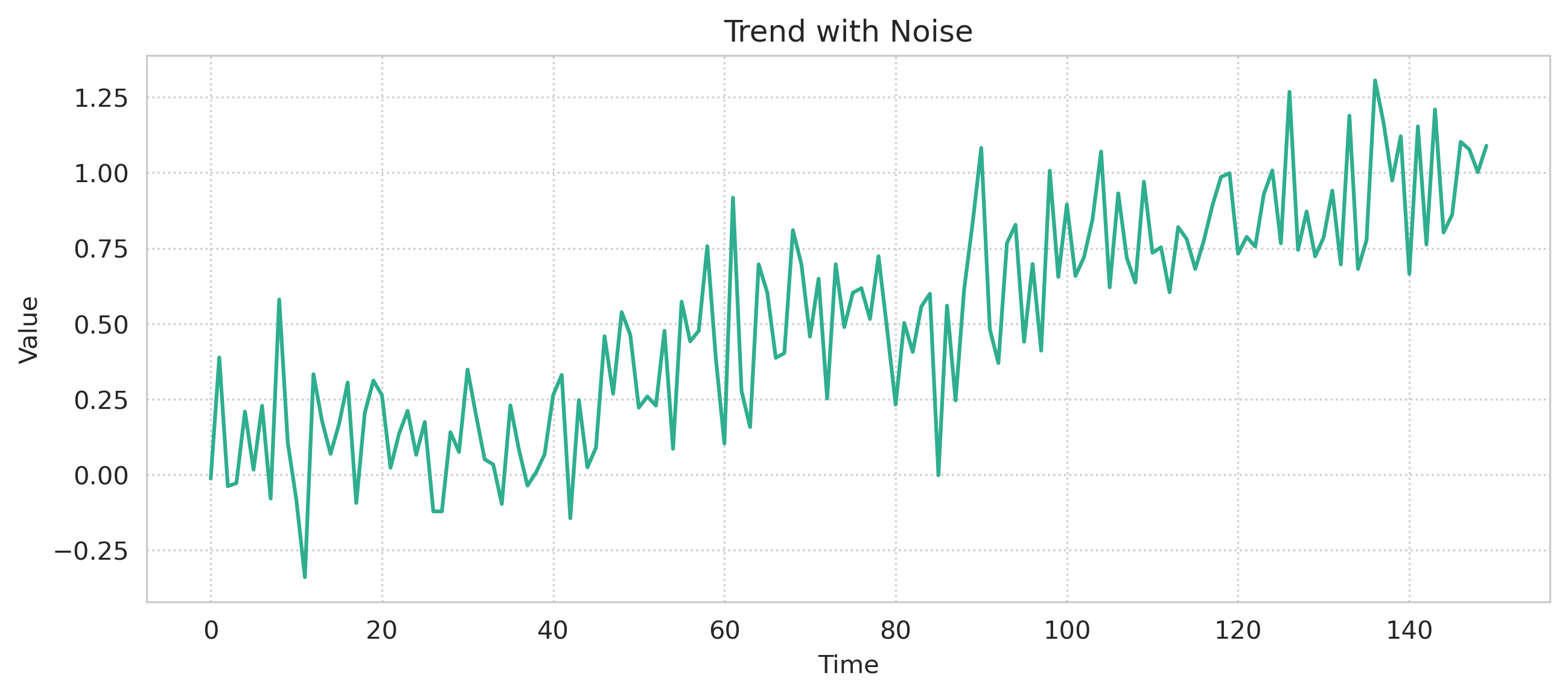
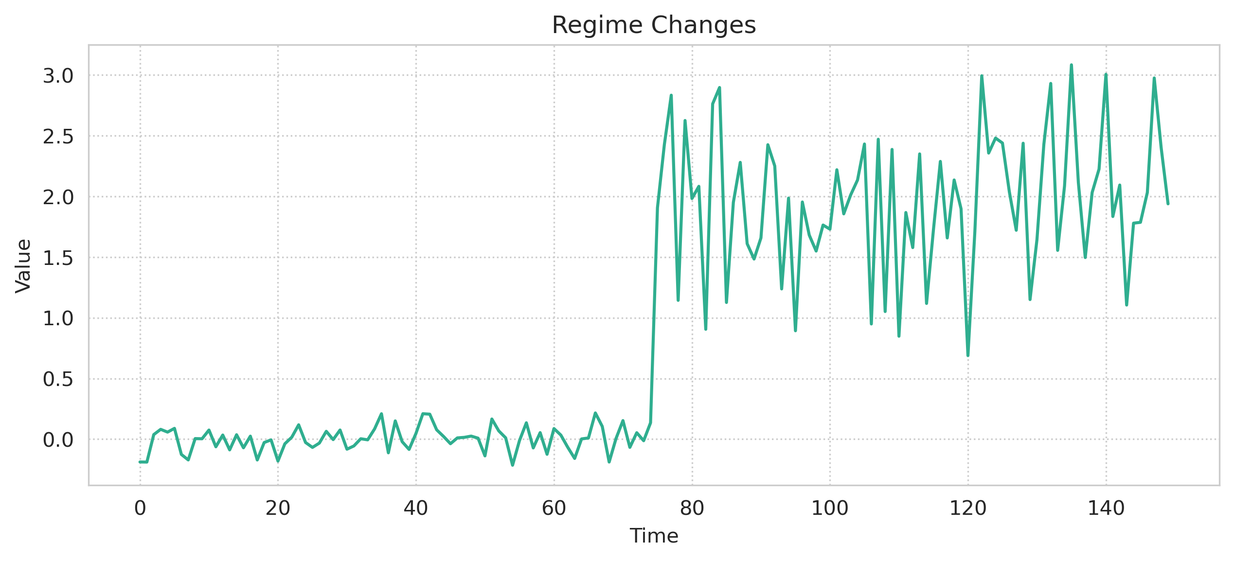
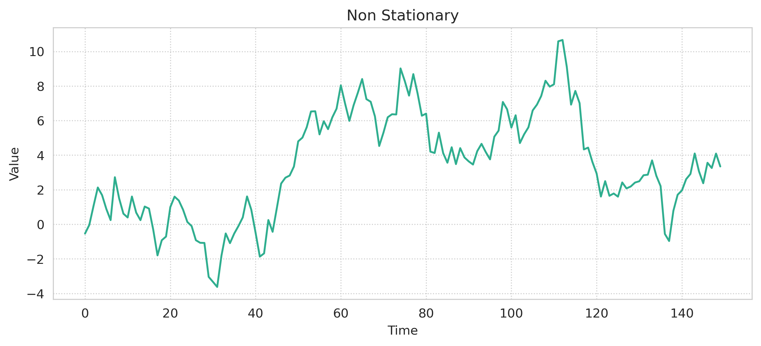
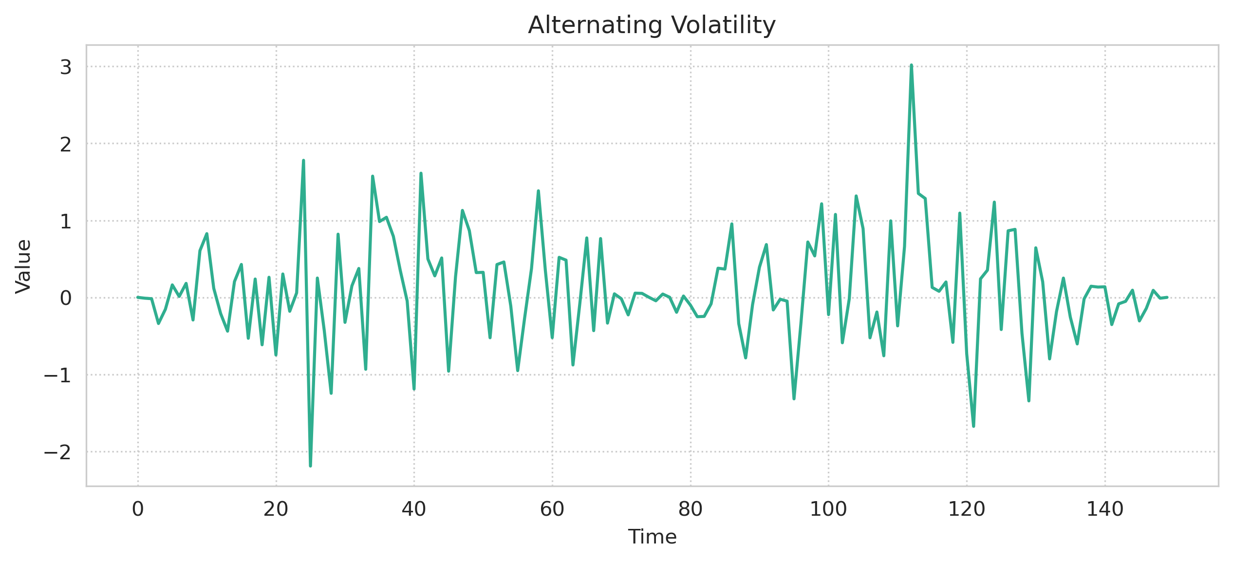
Figure 1: Example synthetically generated time series.

4 Time Series Benchmark Tasks

Our evaluation framework is designed to assess the LLMs’ capabilities in analyzing time series across the dimensions in our taxonomy (Sec. 3.1). The evaluation includes four primary tasks:

Feature Detection

This task evaluates the LLMs’ ability to identify the presence of specific features within a time series, such as trend, seasonality, or anomalies. For instance, given a time series dataset with an upward trend, the LLM is queried to determine if a trend exists. Queries are structured as yes/no questions to assess the LLMs’ ability to recognize the presence of specific time series features, such as "Is a trend present in the time series?"

Feature Classification

Once a feature is detected, this task assesses the LLMs’ ability to classify the feature accurately. For example, if a trend is present, the LLM must determine whether it is upward, downward, or non-linear. This task involves a QA setup where LLMs are provided with definitions of sub-features within the prompt. Performance is evaluated based on the correct identification of sub-features, using the F1 score to balance precision and recall. This task evaluates the models’ depth of understanding and ability to distinguish between similar but distinct phenomena.

Information Retrieval

Evaluates the LLMs’ accuracy in retrieving specific data points, such as values on a given date.

Arithmetic Reasoning

Focuses on quantitative analysis tasks, such as identifying minimum or maximum values. Accuracy and Mean Absolute Percentage Error (MAPE) are used to measure performance, with MAPE offering a precise evaluation of the LLMs’ numerical accuracy.

Additionally, to account for nuanced aspects of time series analysis, we propose in Sec. 5.2 to study the influence of multiple factors, including time series formatting, location of query data point in the time series and time series length.

5 Performance Metrics and Factors

5.1 Performance Metrics

We employ the following metrics to report the performance of LLMs on various tasks.

F1 Score

Applied to feature detection and classification, reflecting the balance between precision and recall.

Accuracy

Used for assessing the information retrieval and arithmetic reasoning tasks.

Mean Absolute Percentage Error (MAPE)

Employed for numerical responses in the information retrieval and arithmetic reasoning tasks, providing a measure of precision in quantitative analysis.

5.2 Performance Factors

We identified various factors that could affect the performance of LLMs on time series understanding, for each we designed deep-dive experiments to reveal the impacts.

Time Series Formatting

Extracting useful information from raw sequential data as in the case of numerical time series is a challenging task for LLMs. The tokenization directly influences how the patterns are encoded within tokenized sequences Gruver et al. (2023), and methods such as BPE separate a single number into tokens that are not aligned. On the contrary, Llama2 has a consistent tokenization of numbers, where it splits each digit into an individual token, which ensures consistent tokenization of numbers (Liu and Low, 2023). We study different time series formatting approaches to determine if they influence the LLMs performance to capture the time series information. In total we propose 9 formats, ranging from simple CSV to enriched formats with additional information.

Time Series Length

We study the impact that the length of the time series has in the retrieval task. Transformer-based models use attention mechanisms to weigh the importance of different parts of the input sequence. Longer sequences can dilute the attention mechanism’s effectiveness, potentially making it harder for the model to focus on the most relevant parts of the text Vaswani et al. (2017).

Position Bias

Given a retrieval question, the position of where the queried data point occurs in the time series might impact the retrieval accuracy. Studies have discovered recency bias Zhao et al. (2021) in the task of few-shot classification, where the LLM tends to repeat the label at the end. Thus, it’s important to investigate whether LLM exhibits similar bias on positions in the task of time series understanding.

6 Experiments

6.1 Experimental setup

6.1.1 Models

We evaluate the following LLMs on our proposed framework: 1) GPT4. (Achiam et al., 2023) 2) GPT3.5. 3) Llama2-13B Touvron et al. (2023), and 4) Vicuna-13B Chiang et al. (2023). We selected two open-source models, Llama2 and Vicuna, each with 13 billion parameters, the version of Vicuna is 1.5 was trained by fine-tuning Llama2. Additionally we selected GPT4 and GPT3.5 where the number of parameters is unknown. In the execution of our experiments, we used an Amazon Web Services (AWS) g5.12xlarge instance, equipped with four NVIDIA A10G Tensor Core GPUs, each featuring 24 GB of GPU RAM. This setup was essential for handling both extensive datasets and the computational demands of LLMs.

6.1.2 Prompts

The design of prompts for interacting with LLMs is separated into two approaches: retrieval/arithmetic reasoning and detection/classification questioning.

Time series characteristics

To evaluate the LLM reasoning over time series features, we use a two-step prompt with an adaptive approach, dynamically tailoring the interaction based on the LLM’s responses. The first step involves detection, where the model is queried to identify relevant features within the data. If the LLM successfully detects a feature, we proceed with a follow-up prompt, designed to classify the identified feature between multiple sub-categories. For this purpose, we enrich the prompts with definitions of each sub-feature (e.g. up or down trend), ensuring a clearer understanding and more accurate identification process. An example of this two-turn prompt is shown in Fig. 2. The full list can be found in Sec. F of the supplementary.

Information Retrieval/Arithmetic Reasoning

We test the LLM’s comprehension of numerical data represented as text by querying it for information retrieval and numerical reasoning, as exemplified in Fig. 3 and detailed in the supplementary Sec. F.

Figure 2: Example of multi-turn prompt template used for time series feature detection and classification.

Figure 3: The prompt template used for information retrieval and arithmetic reasoning evaluation.

6.2 Benchmark Results

In Table 2, we display the main results for all tasks outlined in Sec. 4.

Table 2: Performances across all reasoning tasks (Bold indicates best performance).

	Metric	GPT4	GPT3.5	Llama2	Vicuna
Univariate time series characteristics
Feature detection
Trend	F1score	0.88	0.43	0.54	0.60
Seasonality	F1score	0.98	0.70	0.71	0.47
Outlier	F1score	0.53	0.53	0.46	0.53
Struct. break	F1score	0.67	0.56	0.43	0.52
Volatility	F1score	0.45	0.50	0.45	0.50
Fat Tails	F1score	0.43	0.51	0.31	0.44
Stationarity	F1score	0.31	0.31	0.31	0.31
Feature classification
Trend	F1score	0.98	0.47	0.41	0.61
Seasonality	F1score	0.25	0.15	0.17	0.20
Outlier	F1score	0.67	0.17	0.07	0.28
Struct. break	F1score	0.34	0.48	0.31	0.36
Volatility	F1score	0.13	0.16	0.10	0.23
Multivariate time series characteristics
Fixed Corr.	F1score	0.40	0.42	0.30	0.32
Lagged Corr.	F1score	0.44	0.47	0.22	0.33
Changing Corr.	F1score	0.43	0.41	0.23	0.41
Information Retrieval
Value on Date	Acc	1.00	0.94	0.38	0.48
Value on Date	MAPE	0.00	0.10	0.65	0.78
Arithmetic Reasoning
Min Value	Acc	1.00	0.99	0.58	0.66
	MAPE	0.00	0.04	16.18	12.24
Min Date	Acc	0.98	0.94	0.38	0.55
Max Value	Acc	0.97	0.92	0.56	0.46
	MAPE	0.01	0.08	0.95	0.74
Max Date	Acc	0.96	0.88	0.46	0.42

The results for univariate time series feature detection and classification tasks illustrate GPT4’s robustness in trend and seasonality detection, substantially outperforming Llama2 and Vicuna. However, the detection of structural breaks and volatility presents challenges across all models, with lower accuracy scores.

GPT4 excels in trend classification tasks, demonstrating superior performance. However, in classifying seasonality, outliers, and structural breaks, performance is mixed, with Vicuna sometimes surpassing Llama2, highlighting the distinct strengths of each model. Figure 4 summarizes the accuracy performance for the information retrieval and arithmetic reasoning tasks, and F1 score for the feature detection and classification tasks for all models.

In multivariate time series feature detection and classification tasks, all models achieve moderate accuracy, suggesting potential for enhancement in intricate multivariate data analysis.

For information retrieval tasks, GPT4 outperforms GPT3.5 and other models, achieving perfect accuracy in identifying the value on a given date. It also maintains a low Mean Absolute Percentage Error (MAPE), indicative of its precise value predictions. The arithmetic reasoning results echo these findings, with GPT4 displaying superior accuracy, especially in determining minimum and maximum values within a series.

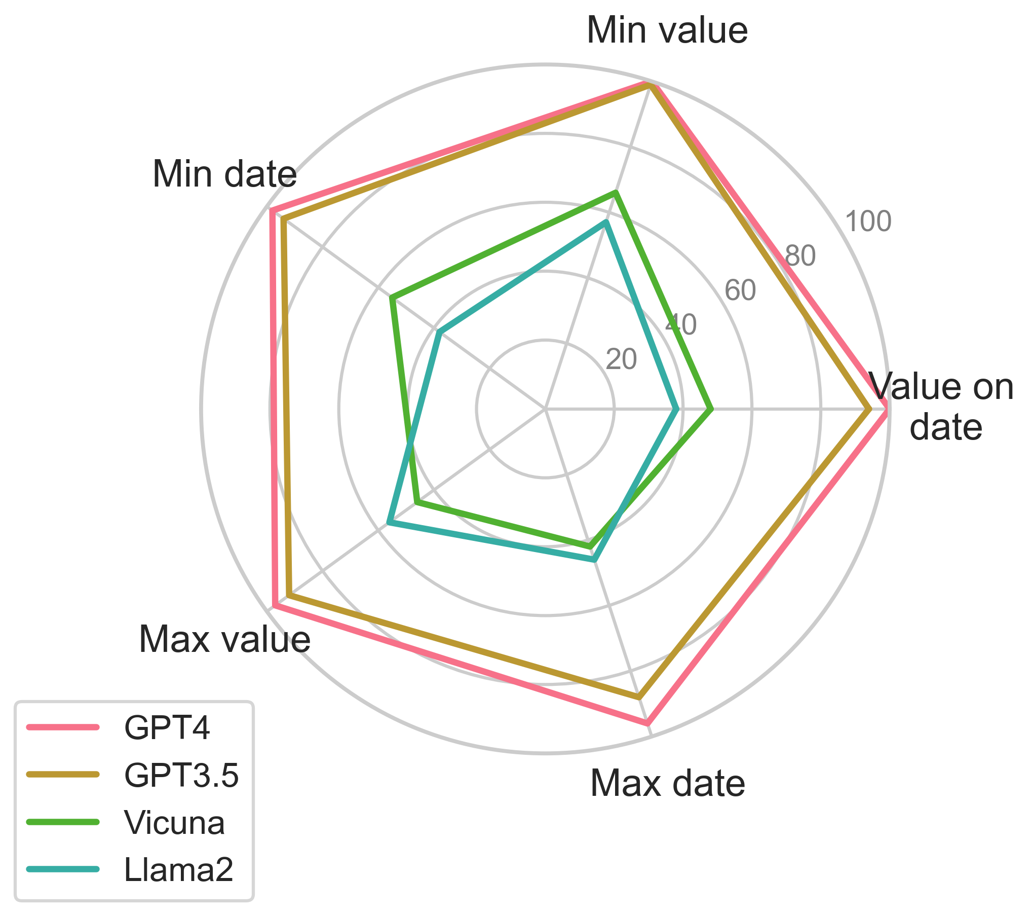
(a) IR and arithmetic reasoning

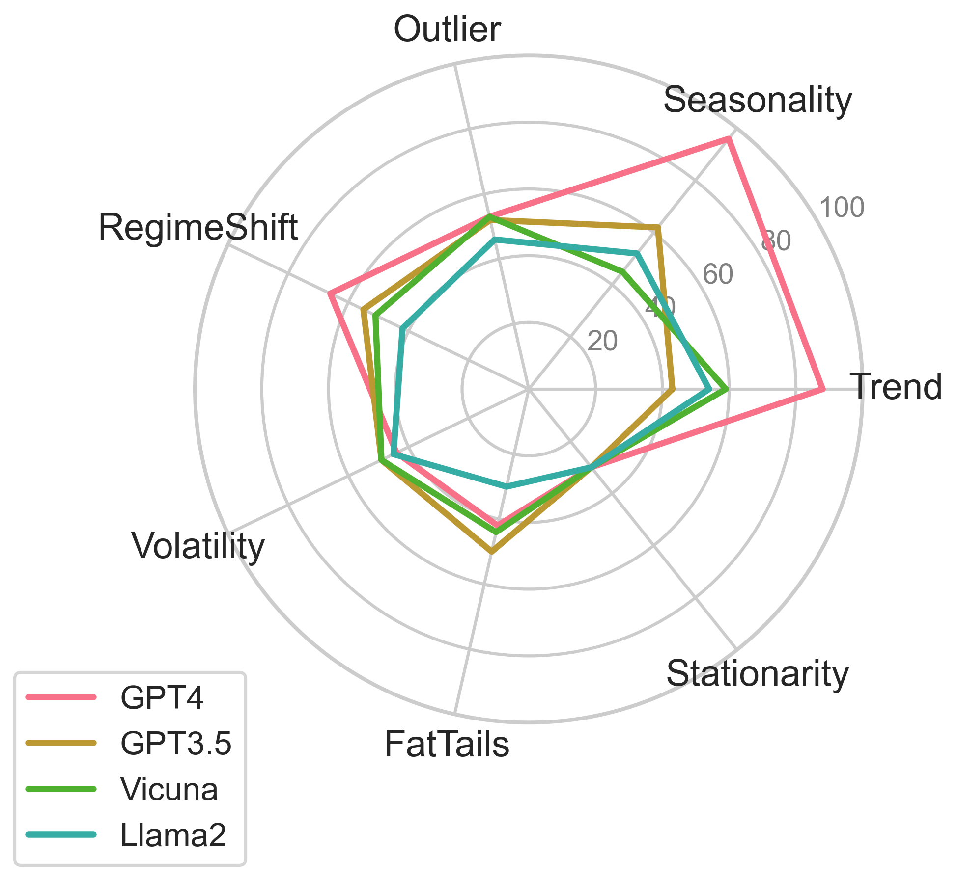
(b) Feature detection

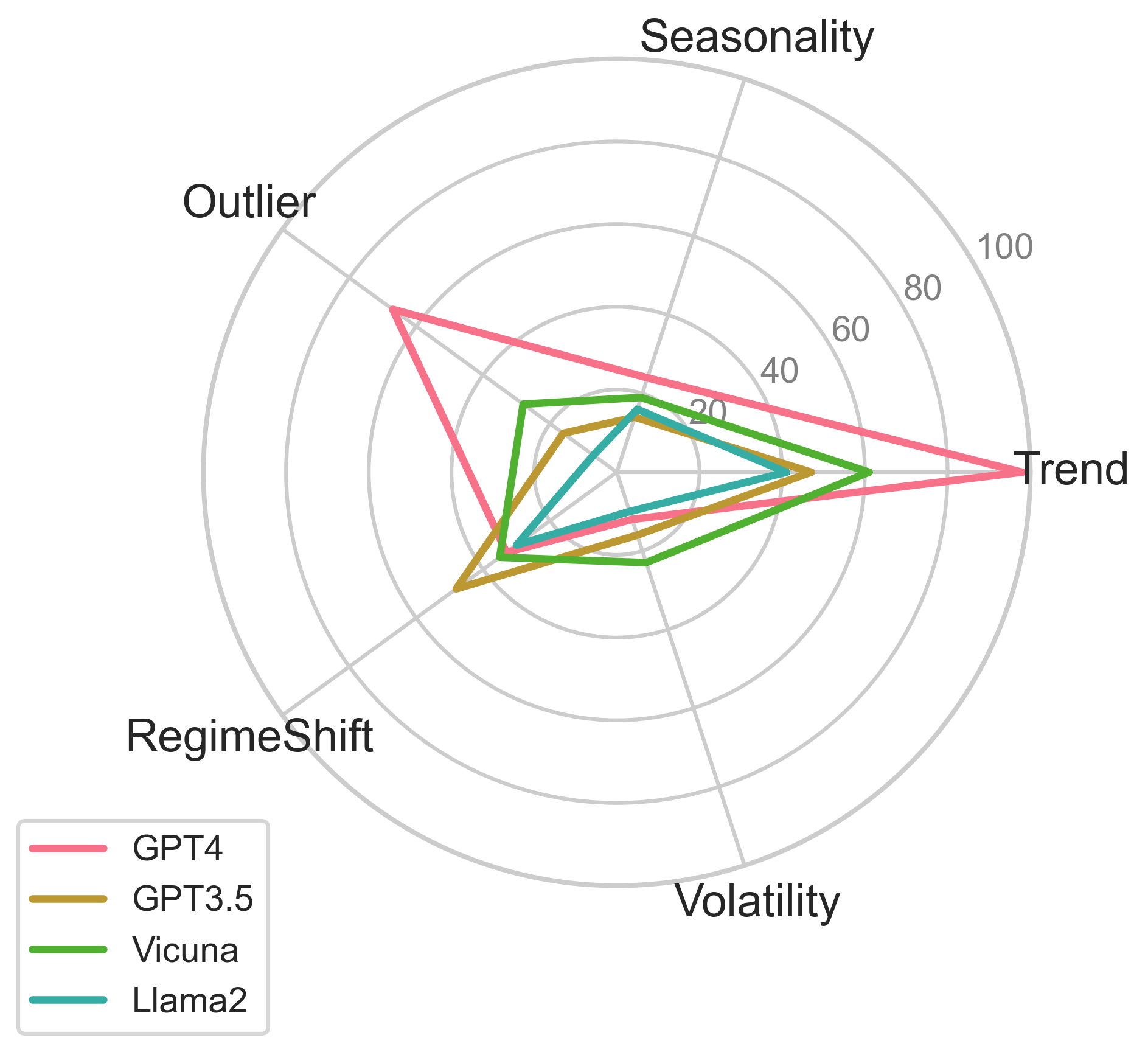
(c) Feature classification

Figure 4: Feature detection and classification scores of GPT4, GPT3.5, Vicuna and Llama2.

6.3 Deep Dive on Performance Factors

Time Series Formatting

We present four formatting approaches in this section, csv, which is a common comma separated value, plain where the time series is formatted as Date:YYYY-MM-DD,Value:num for each pair date-value. We also use the formatting approach proposed by Gruver et al. (2023) which we denominate spaces that adds blank spaces between each digit of the time series, tokenizing each digit individually, and symbol, an enriched format where we add a column to the time series with arrows indicating if the value has moved up, down or remained unchanged. Examples of every approach can be found in Sec. E in the Appendix.

Table 3 shows the results for the four time series formatting strategies. For the full results, please refer to Tables 10 and 9. For the information retrieval and arithmetic reasoning tasks, the plain formatting yields better results across all models. This approach provides more structure to the input, and outperforms other formats in a task where the connection between time and value is important. For the detection and classification tasks, the plain formatting does not yield better results. Interestingly the symbol formatting that adds an additional column to the time series yields better results in the trend classification task. This means that the LLMs can correctly map the symbol to the time series movement and use it to achieve the best performance in trend classification. Furthermore, GPT3.5 leverages this additional information in the trend and anomalies datasets but not in the seasonality dataset.

	GPT3.5				Llama2				Vicuna
	csv	plain	spaces	symbol	csv	plain	spaces	symbol	csv	plain	spaces	symbol
Min value	0.98	0.99	0.79	0.98	0.55	0.58	0.20	0.58	0.63	0.67	0.17	0.62
Min date	0.94	0.95	0.69	0.93	0.28	0.39	0.09	0.29	0.50	0.55	0.13	0.49
Max value	0.92	0.92	0.54	0.94	0.48	0.56	0.05	0.52	0.49	0.46	0.01	0.50
Max date	0.88	0.88	0.51	0.89	0.34	0.46	0.04	0.41	0.38	0.42	0.07	0.41
Value on date	0.94	0.94	0.82	0.94	0.39	0.38	0.07	0.34	0.36	0.48	0.09	0.41
Trend det	0.42	0.41	0.42	0.42	0.51	0.44	0.34	0.40	0.51	0.49	0.54	0.45
Trend class	0.74	0.55	0.53	0.92	0.41	0.48	0.43	0.62	0.49	0.58	0.44	0.64
Season det	0.61	0.77	0.63	0.47	0.55	0.24	0.40	0.50	0.47	0.47	0.53	0.54
Season class	0.27	0.19	0.17	0.18	0.11	0.13	0.08	0.10	0.14	0.14	0.14	0.15
Outlier det	0.55	0.52	0.52	0.62	0.44	0.35	0.41	0.47	0.49	0.53	0.54	0.49
Outlier class	0.17	0.17	0.17	0.17	0.13	0.14	0.14	0.08	0.19	0.14	0.14	0.08

Table 3: Top: Time series feature detection and classification performance measured with F1 score. Bottom: Time series information retrieval and arithmetic reasoning performance measured by accuracy for different time series formats. (Bold indicates best performance)

Time Series Length

Figure 5 shows the performance of GPT3.5, Llama2 and Vicuna on three datasets, trend, seasonality and outliers wich have time series with different lengths. We observe that GPT3.5 retrieval performance degrades slowly with increasing sequence length. Llama2 and and Vicuna suffer a more steep degradation especially from time series of length 30 steps to 60 steps; for longer sequences the degradation in performance becomes linear.

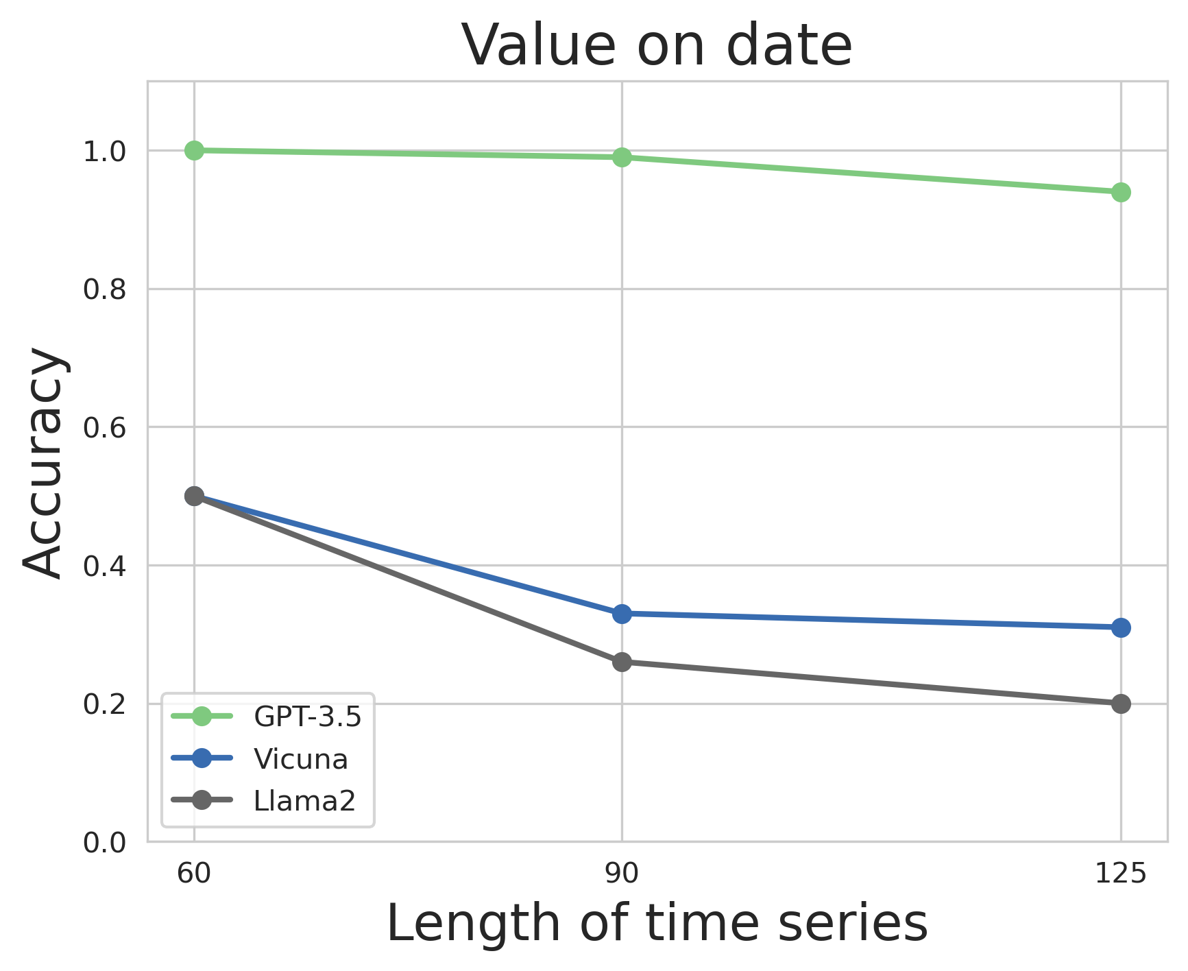
(a) Trend

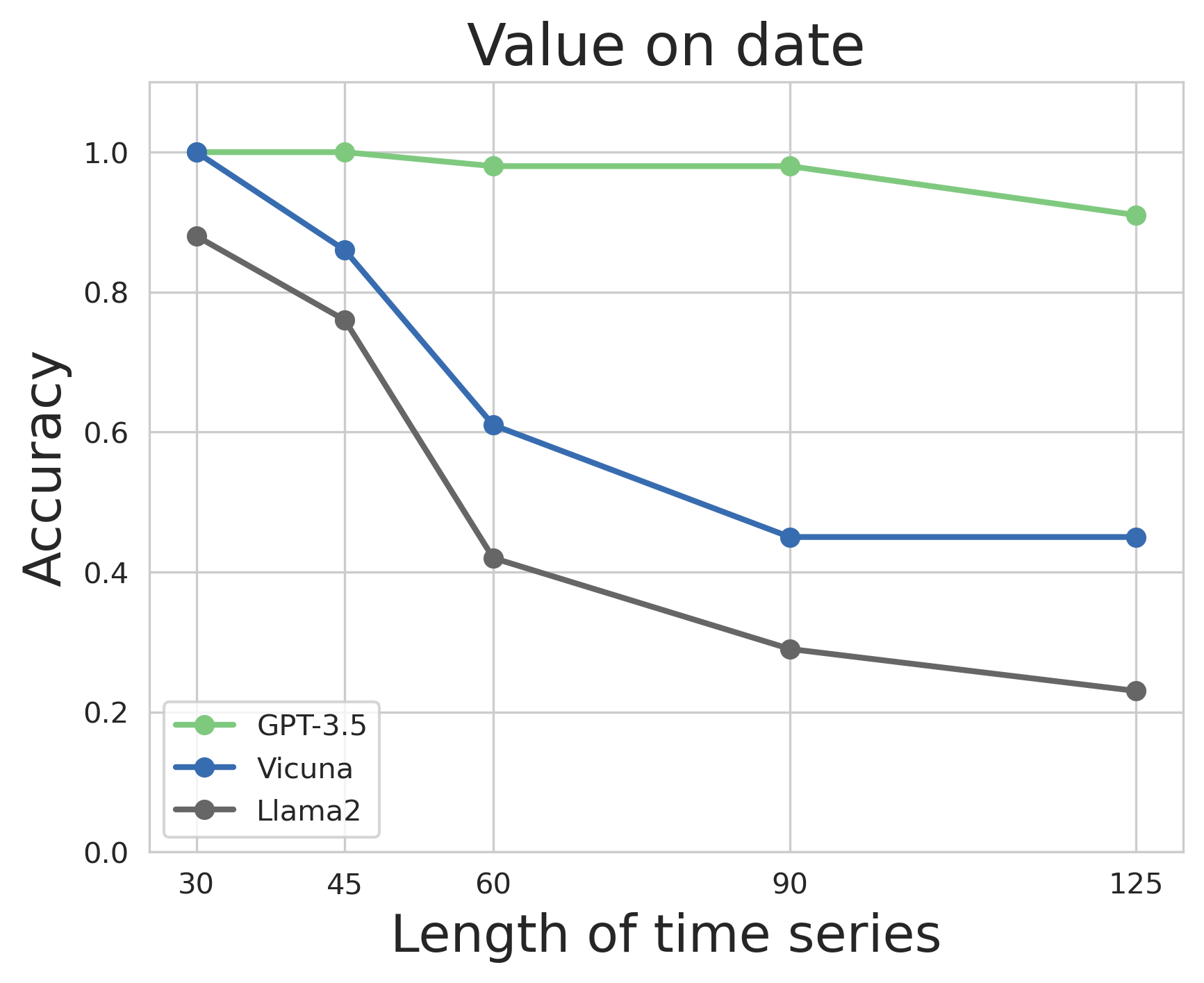
(b) Seasonality

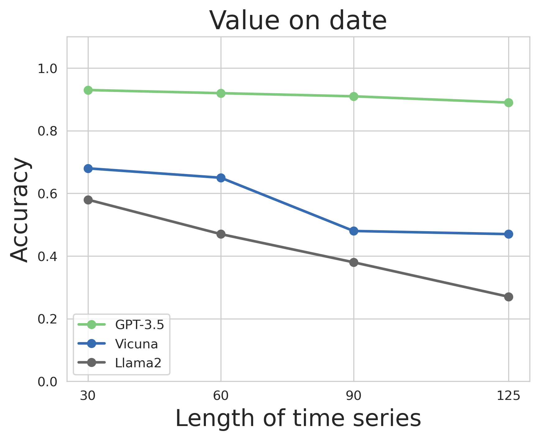
(c) Outliers

Figure 5: Retrieval performance for different time series lengths.

Position Bias

We carry out a series of experiments to determine how the position of the target value affects task performance across various types of time series data. We address progressively more complex objectives: 1) identifying the presence of a value in a time series without a specified date (D.1); 2) retrieving a value corresponding to a specific date (D.2); and 3) identifying the minimum and maximum values (D.3). We cover a range of time series data, from monotonic series without noise to those with noise, sinusoidal patterns, data featuring outliers (spikes), and Brownian motion scenarios, each adding a layer of complexity. We examine how the position of the target value within the four quadrants — 1st, 2nd, 3rd, and 4th— affects the efficacy of these tasks across the varied time series landscapes. This approach helps reveal the influence of position on different LLMs (GPT3.5, Llama2, and Vicuna) in the task of time series understanding.

We consider the presence of position bias when the maximum performance gap between quadrants exceeds 10%. Given this criterion, our analysis provides the following key takeaways on position bias impacting LLM performance across the defined tasks:

• Pronounced position bias is observed across all tasks and LLMs

  • GPT models show significant bias exclusively in complex tasks that involve arithmetic reasoning.

  • Both Llama2 and Vicuna demonstrate position biases across all tasks, from the simplest to the most complex ones.

• The degree of complexity in the time series data tends to increase the extent of position bias observed within each task.

Refer to Section D in the appendix, where we offer a detailed analysis of position bias across each task to further substantiate these conclusions.

7 Conclusion

In conclusion, we provide a critical examination of general-purpose Large Language Models (LLMs) in the context of time series understanding. Through the development of a comprehensive taxonomy of time series features and the synthesis of a diverse dataset that encapsulates these features, we have laid a solid foundation for evaluating the capabilities of LLMs in understanding and interpreting time series data. Our systematic evaluation sheds light on the inherent strengths and limitations of these models, offering valuable insights for practitioners aiming to leverage LLMs in time series understanding. Recognizing the areas of weakness and strength in general-purpose LLMs’ current capabilities allows for targeted enhancements, ensuring that these powerful models can be more effectively adapted to specific domains.

8 Limitations

In this section, we detail the key limitations of our study and suggest pathways for future research.

Time series data frequently intersects with data from other domains. In the financial industry, for instance, analysis often combines time series data like stock prices and transaction volumes with supplementary data types such as news articles (text), economic indicators (tabular), and market sentiment analysis (textual and possibly visual). Our future work aims to delve into how LLMs can facilitate the integration of multimodal data, ensure cohesive data modality alignment within the embedding space, and accurately interpret the combined data insights.

Currently, our application of LLMs in time series analysis is primarily focused on comprehending time series features. However, the lack of interpretability mechanisms within our framework stands out as a significant shortcoming. Moving forward, we plan to focus on developing and integrating interpretability methodologies for LLMs specifically tailored to time series data analysis contexts.

Appendix A Synthetic Time Series Dataset

A.1 Univariate Time Series

The primary characteristics considered in our univariate dataset include:

1. Trend We generated time series data to analyze the impact of trends on financial market behavior. This dataset encompasses linear and quadratic trends. For linear trends, each series follows a simple linear equation a * t + b, where a (the slope) varies between 0.1 and 1, multiplied by the direction of the trend, and b (the intercept) is randomly chosen between 100 and 110. This simulates scenarios of steadily increasing or decreasing trends. For quadratic trends, the series is defined by $a*t^{2}+b*t+c$, with a varying between 0.01 and 0.05 (again adjusted for trend direction), b between 0 and 1, and c between 0 and 10, or adjusted to ensure non-negative values. The quadratic trend allows us to simulate scenarios where trends accelerate over time, either upwards or downwards, depending on the direction of the trend. This approach enables the exploration of different types of trend behaviors in financial time series, from gradual to more dynamic changes, providing a comprehensive view of trend impacts in market data.

2. Seasonality In our study, we meticulously crafted a synthetic dataset to explore and analyze the dynamics of various types of seasonality within time series data, aiming to closely mimic the complexity found in real-world scenarios. This dataset is designed to include four distinct types of seasonal patterns, offering a broad spectrum for analysis: (1) Fixed Seasonal Patterns, showcasing regular and predictable occurrences at set intervals such as daily, weekly, or monthly, providing a baseline for traditional seasonality; (2) Varying Amplitude, where the strength or magnitude of the seasonal effect fluctuates over time, reflecting phenomena where seasonal influence intensifies or diminishes; (3) Shifting Seasonal Pattern, characterized by the drift of seasonal peaks and troughs over the timeline, simulating scenarios where the timing of seasonal effects evolves; and (4) Multiple Seasonal Patterns, which presents a combination of different seasonal cycles within the same series, such as overlapping daily and weekly patterns, to capture the complexity of real-world data where multiple seasonalities interact. This diverse dataset serves as a foundation for testing the sensitivity and adaptability of analytical models to detect and quantify seasonality under varying and challenging conditions.

3. Anomalies and outliers refer to observations that significantly deviate from the typical pattern or trend observed in the dataset. The types of outliers included in our generated dataset are: 1) single sudden spike for isolated sharp increases, 2) double and triple sudden spikes for sequences of consecutive anomalies, 3) step spike and level shift for persistent changes, and 4) temporal disruption for sudden interruptions in the pattern. We also include a no outlier category as a control for comparative analysis. Parameters such as the location and magnitude of spikes, the duration and start of step spikes, the placement and size of level shifts, and the initiation and conclusion of temporal disruptions are randomly assigned to enhance the dataset’s diversity and relevance.

4. Structural breaks in time series data signify substantial changes in the model generating the data, leading to shifts in parameters like mean, variance, or correlation. These are broadly classified into two types: parameter shifts and regime shifts, with a third category for series without breaks. Parameter shifts involve changes in specific parameters such as mean or variance, including sub-types like mean shifts, variance shifts, combined mean-variance shifts, seasonality amplitude shifts, and autocorrelation shifts. Regime shifts represent deeper changes that affect the model’s structure, including: distribution changes (e.g., normal to exponential), stationarity changes (stationary to non-stationary), linearity changes (linear to non-linear models), frequency changes, noise trend changes, error correlation changes, and variance type changes. The occurrence of these shifts is randomly determined within the time series.

5. Volatility We generated synthetic time series data to simulate various volatility patterns, specifically targeting clustered volatility, leverage effects, constant volatility, and increasing volatility, to mimic characteristics observed in financial markets. For clustered volatility, we utilized a GARCH(1,1) model with parameters $\omega=0.1$, $\alpha=0.05$, and $\beta=0.9$, ensuring the sum of $\alpha$ and $\beta$ remained just below 1 for stationarity, thus capturing high volatility persistence. To simulate the leverage effect, our model increased volatility in response to negative returns, reflecting typical market dynamics. Additionally, we created time series with constant volatility by adding normally distributed random noise (standard deviation of 1) to a cumulative sum of random values, and with increasing volatility by scaling the noise in proportion to the increasing range of the series (scaling factor up to 5 towards the end of the series). The latter was achieved by multiplying the standard deviation of the random noise by a linearly increasing factor, resulting in a volatility profile that progressively intensified. These methodologies enabled us to comprehensively represent different volatility behaviors in financial time series, including constant, increasing, clustered, and leverage-induced volatilities, thereby enriching our analysis with diverse market conditions.

6. Statistical properties Next, we constructed a dataset to delve into significant features of time series data, centering on fat tails and stationarity. The dataset sorts series into four categories: those exhibiting fat tails, characterized by a higher likelihood of extreme values than in a normal distribution; non-fat-tailed, where extreme values are less probable; stationary, with unchanging mean, variance, and autocorrelation; and non-stationary series. Non-stationary series are further divided based on: 1) changing mean: series with a mean that evolves over time, typically due to underlying trends. 2) changing variance: series where the variance, or data spread, alters over time, suggesting data volatility. 3) seasonality: series with consistent, cyclical patterns occurring at set intervals, like seasonal effects. 4) trend and seasonality: series blending both trend dynamics and seasonal fluctuations.

A.2 Multivariate Time Series

For our analysis, we confined each multivariate series sample to include just 2 time series. The main features of our generated multivariate dataset encompass:

1. Correlation involves analyzing the linear relationships between series, which is crucial for forecasting one time series from another when a correlation exists. The randomly selected correlation coefficient quantifies the strength and direction of relationships as positive (direct relationship), negative (inverse relationship), or neutral (no linear relationship) between series.

2. Cross-correlation evaluates the relationship between two time series while considering various time lags, making it valuable for pinpointing leading or lagging relationships between series. For our data generation, the time lag and correlation coefficient are randomly chosen.

3. Dynamic conditional correlation focuses on scenarios where correlations between series vary over time. The points in the time series at which correlation shifts take place are selected randomly.

A.3 Data Examples

Table 4: Examples of the generated univariate time series. The x- and y-axis are intentionally omitted to focus exclusively on the shape and characteristics of the time series.

Trend

(a) Linear trend (b) Quadratic trend (c) Exponential trend (d) No clear trend

Seasonality

(a) Fixed seasonality (b) Varying amplitude (c) Shifting patterns (d) Multiple Seasonalities

Volatility

(a) Constant volatility (b) Increasing volatility (c) Clustered volatility (d) No volatility

Anomalies and Outliers

(a) Double sudden spikes (b) Step spike (c) Level shift (d) Temporal Disruption

Structural breaks

(a) Parameter shift (change in variance) (b) Parameter shift (change in seasonality amplitude) (c) Regime shift (noise trend change) (d) Regime shift (stationarity change)

Statistical properties

(a) Fat tailed (b) Non-stationary (trend) (c) Non-stationary (changing variance over time) (d) Non-stationary (seasonality)

Table 5: Examples of the generated multivariate time series. The x- and y-axis are intentionally omitted to focus exclusively on the shape and characteristics of the time series.

Correlation

(a) Positive correlation (b) Negative correlation (c) No correlation

Cross-correlation

(a) Lagged positive correlation (b) Lagged negative correlation

Dynamic conditional correlation

(a) Positive correlation (first half) (b) Negative correlation (first half) (d) Negative correlation (second half)

Appendix B Additional datasets

Brownian Data: We generate a synthetic time series dataset exhibiting brownian motion. The data consists of 400 samples where each time series has a length of 175. We control for the quadrant in the which the maximum and minimum values appear using rejection sampling i.e. there are 50 samples for which the maximum value in the time series occurs in the first quadrant, 50 samples for which the maximum value appears in the second quadrant, and so on, upto the fourth quadrant. In a similar manner we control for presence of the minimum value in each quadrant.
Outlier Data: We generate a synthetic time series dataset where each time series contains a single outlier which is the either the minimum or maximum values in the time series. The data consists of 400 samples where each time series has a length of 175. We control for the quadrant in the which the maximum and minimum (outlier) values appear using rejection sampling i.e. there are 50 samples for which the maximum value in the time series occurs in the first quadrant, 50 samples for which the maximum value appears in the second quadrant, and so on, upto the fourth quadrant. In a similar manner we control for presence of the minimum value in each quadrant.
Monotone Data: We generate a synthetic time series dataset where each time series is monotonically increasing or decreasing. The data consists of 400 samples (200 each for increasing/decreasing) where each time series has a length of 175.
Monotone (with Noise) Data: We generate a synthetic time series dataset where each time series is increasing or decreasing. The data consists of 400 samples (200 each for increasing/decreasing) where each time series has a length of 175. Note that dataset is different from the Monotone data as the time series samples are not strictly increasing/decreasing.

Appendix C Additional results

C.1 Trend

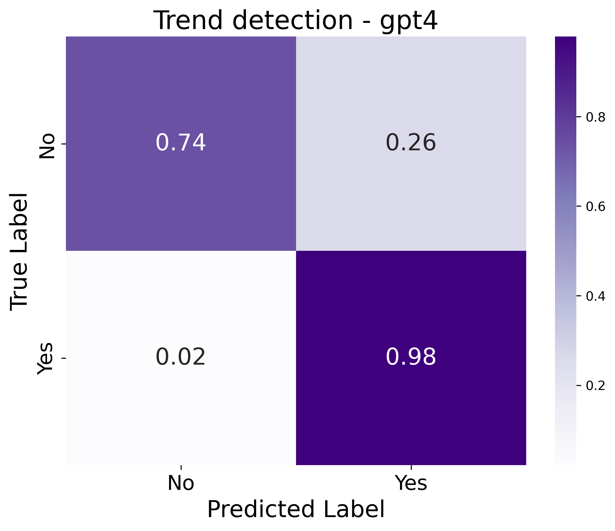
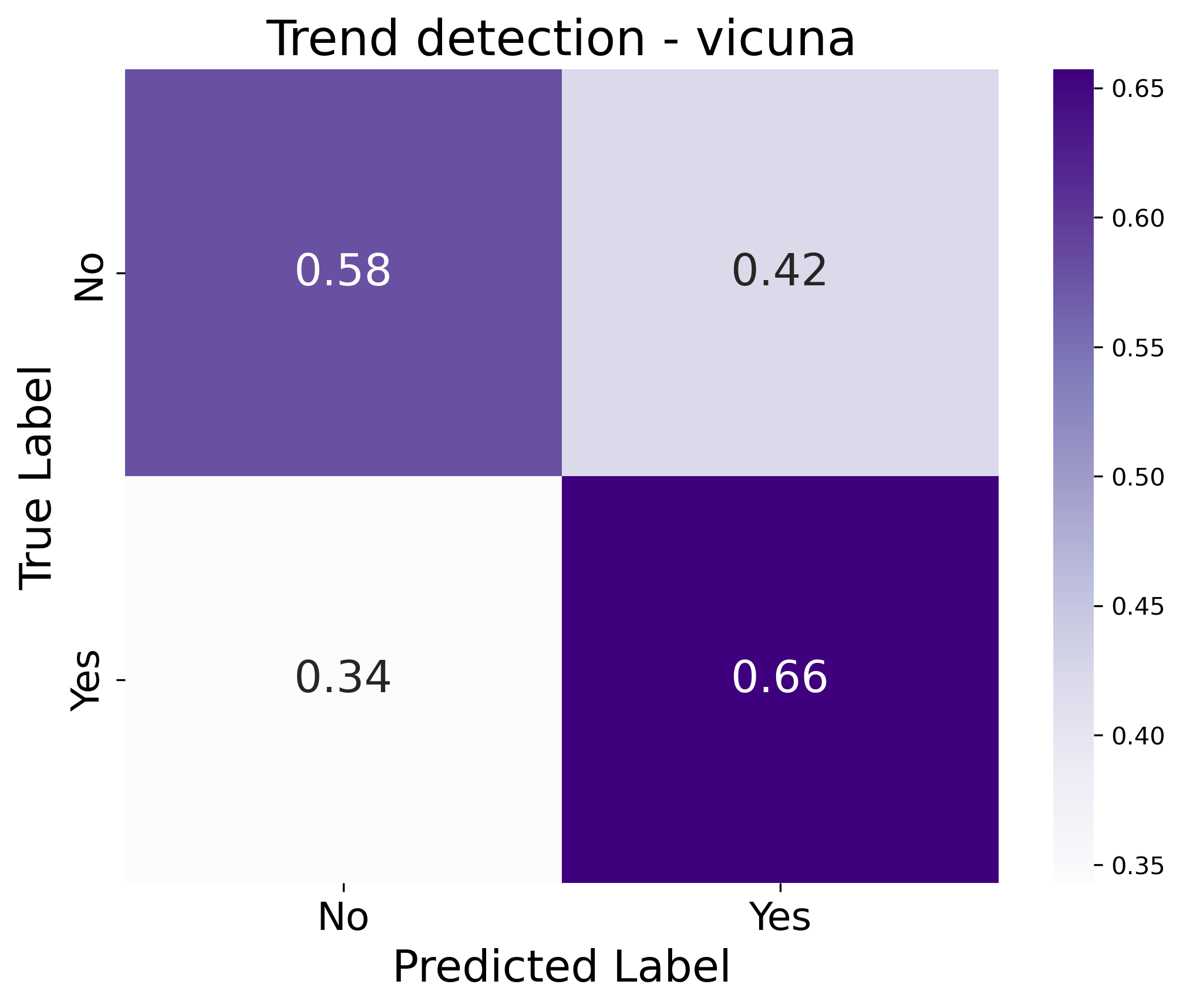
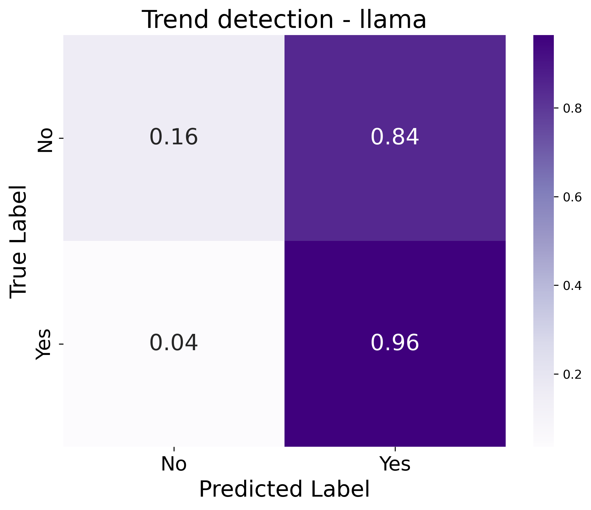
Figure 6: Trend detection

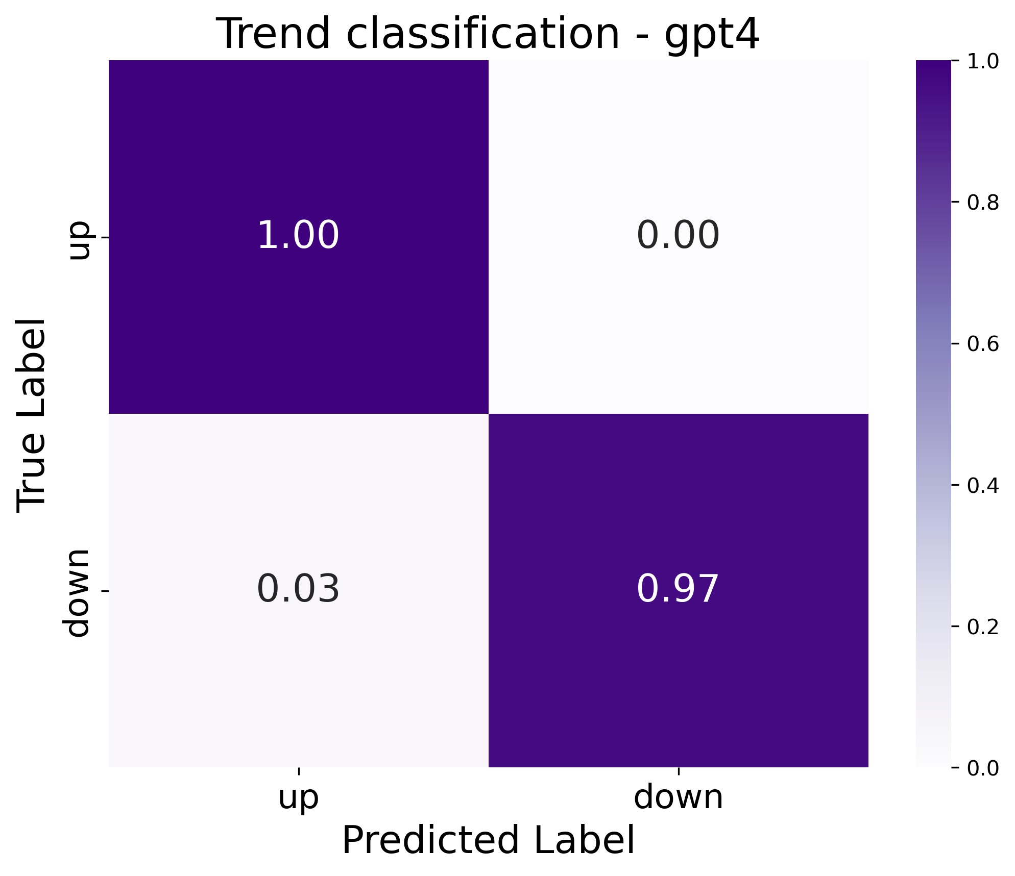
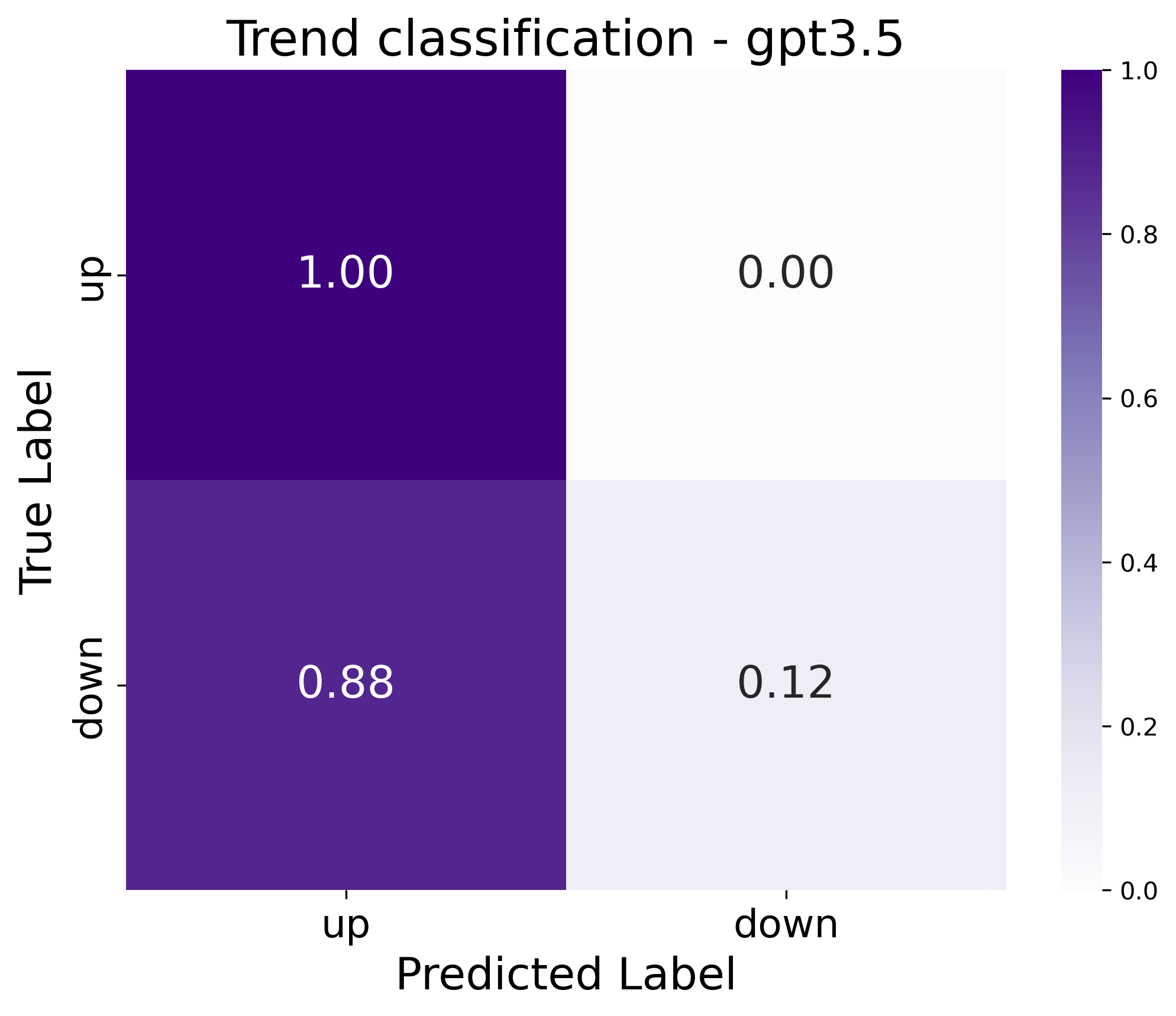
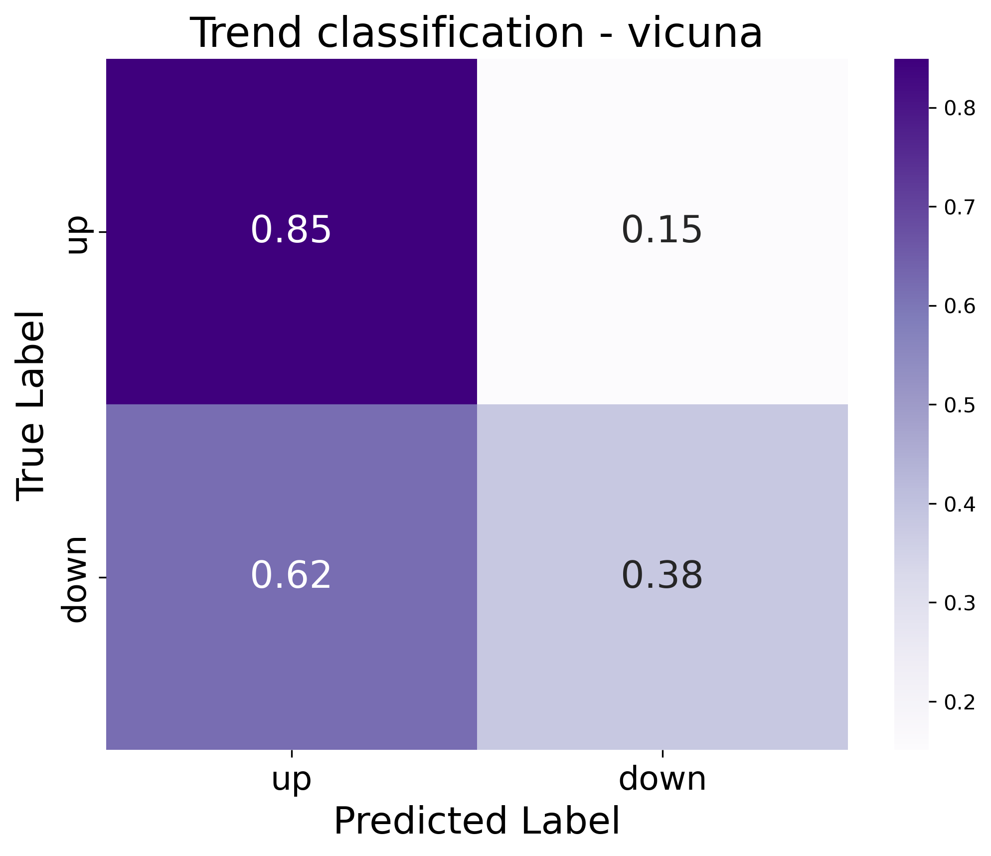
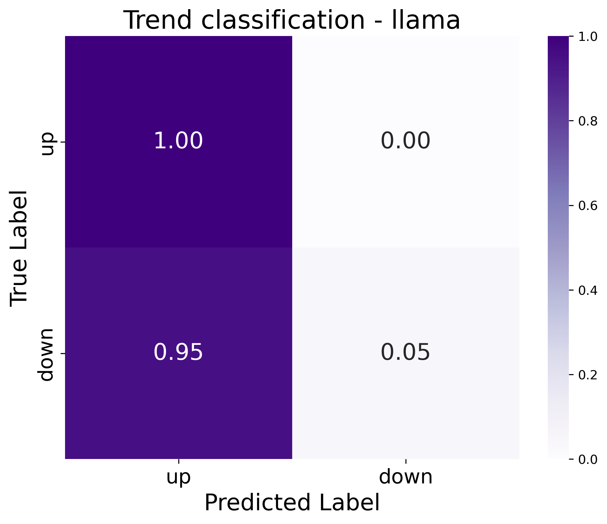
Figure 7: Trend classification

C.2 Seasonality

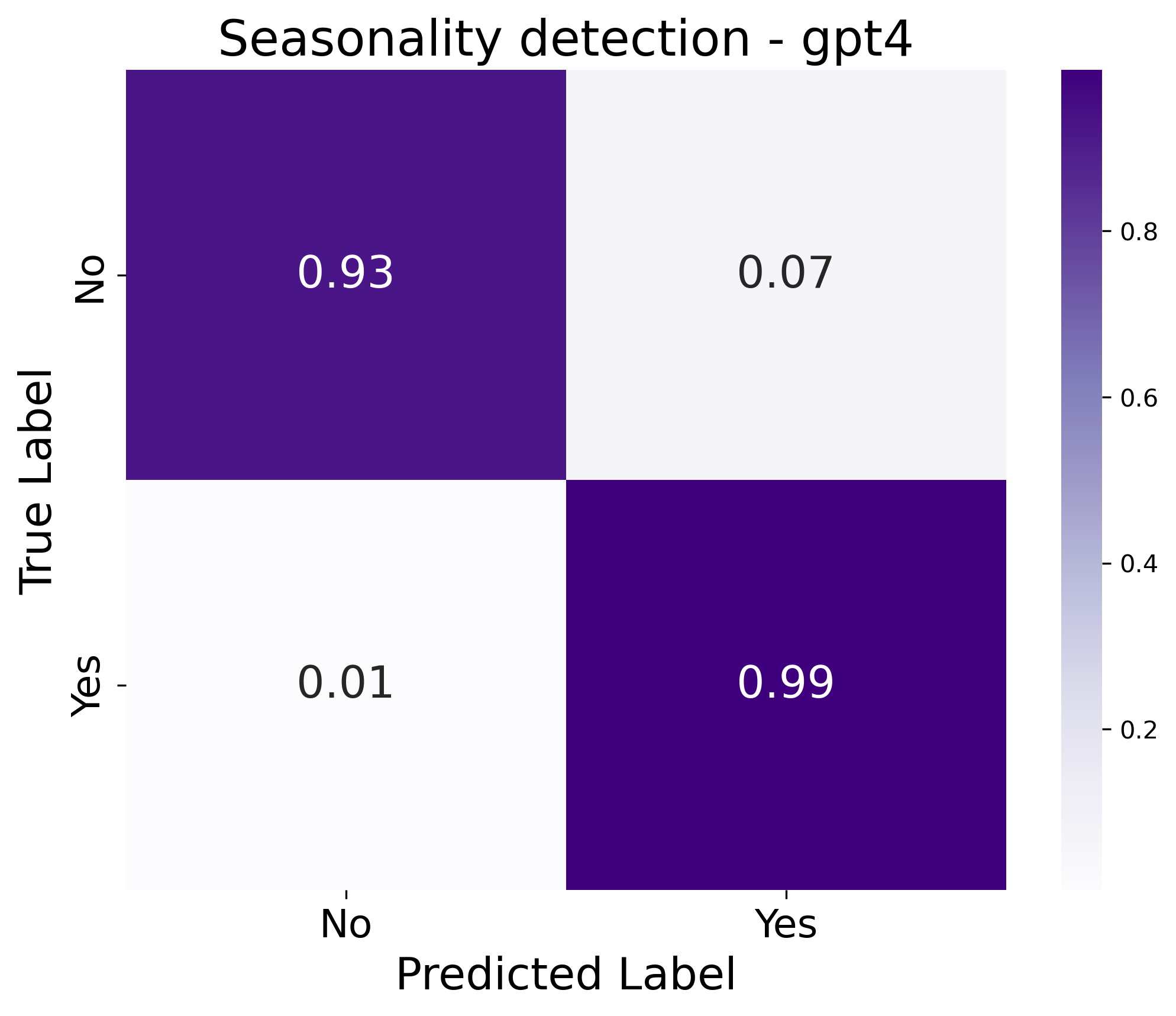
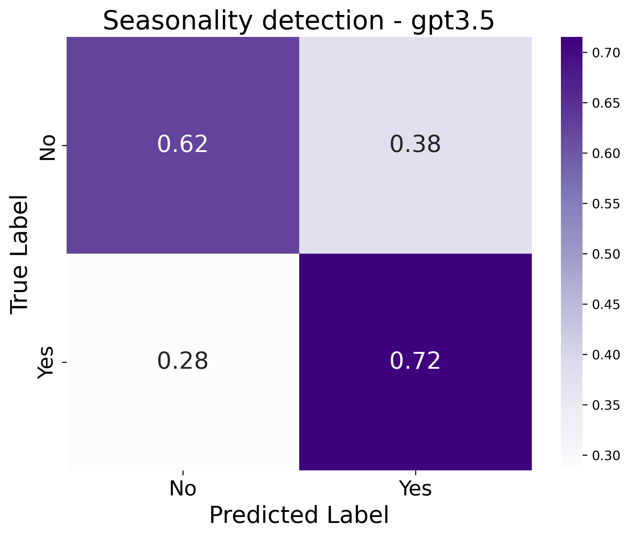
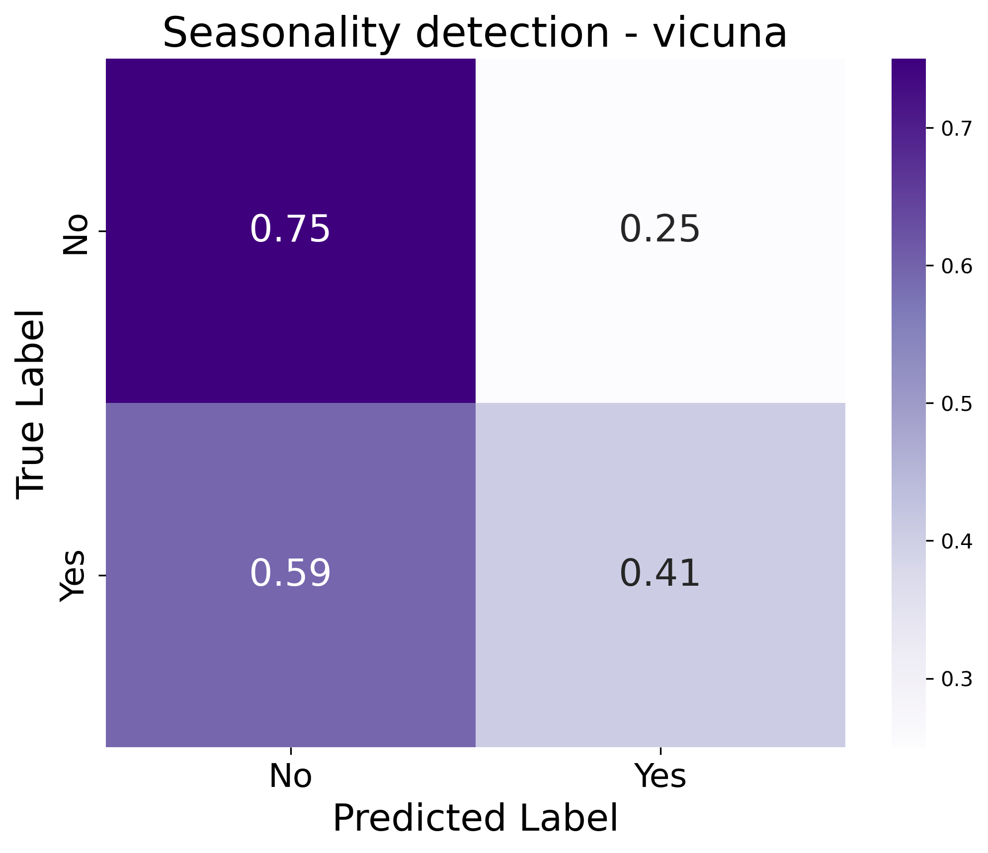
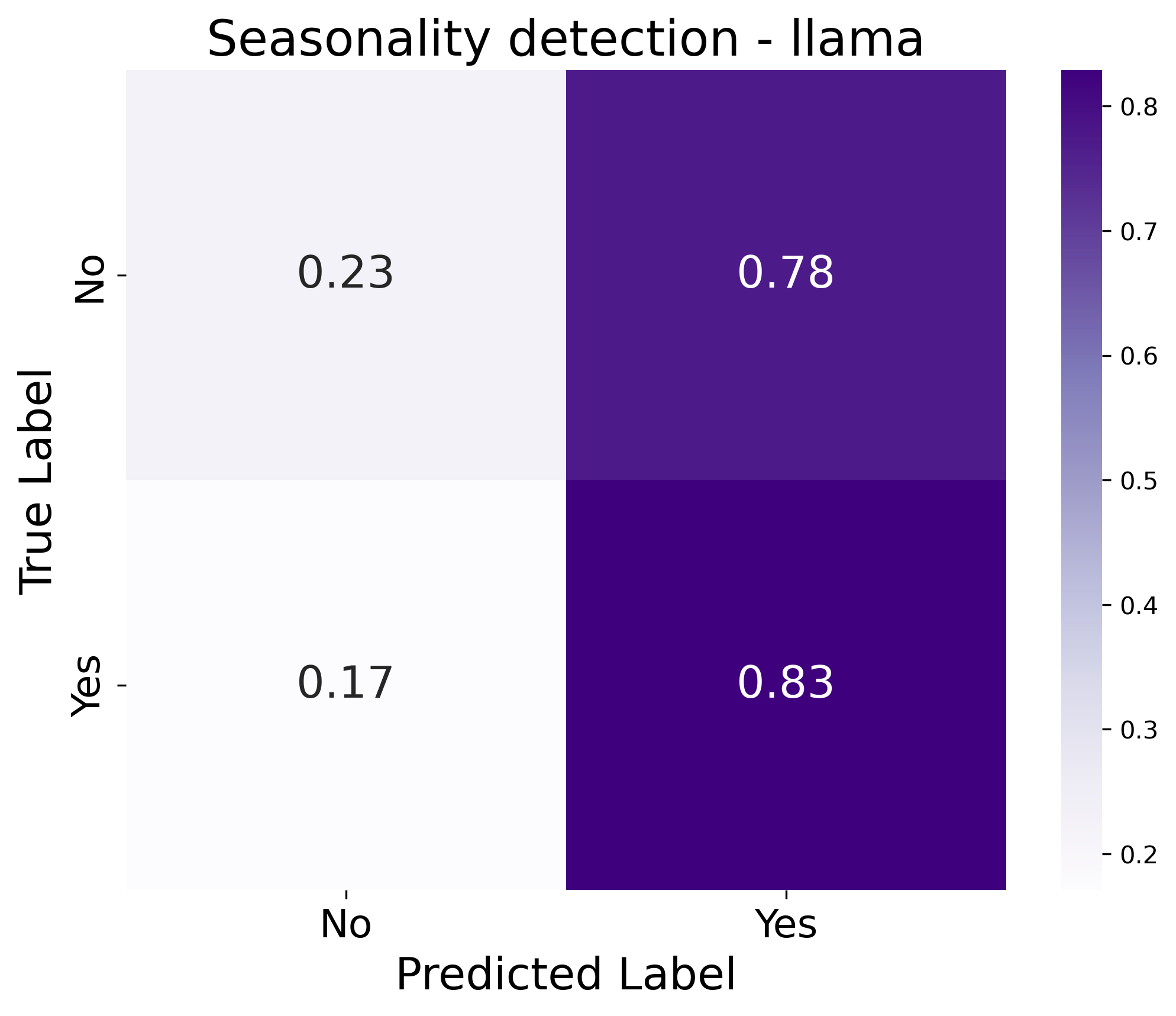
Figure 8: Seasonality detection

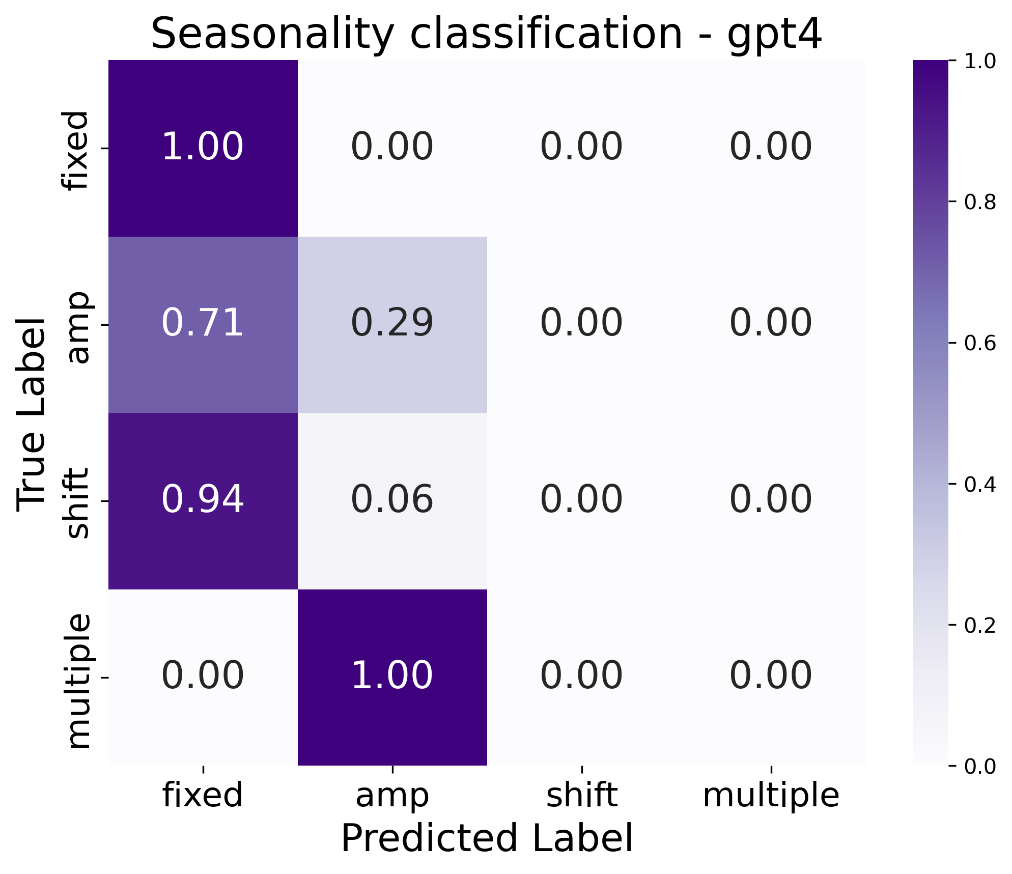
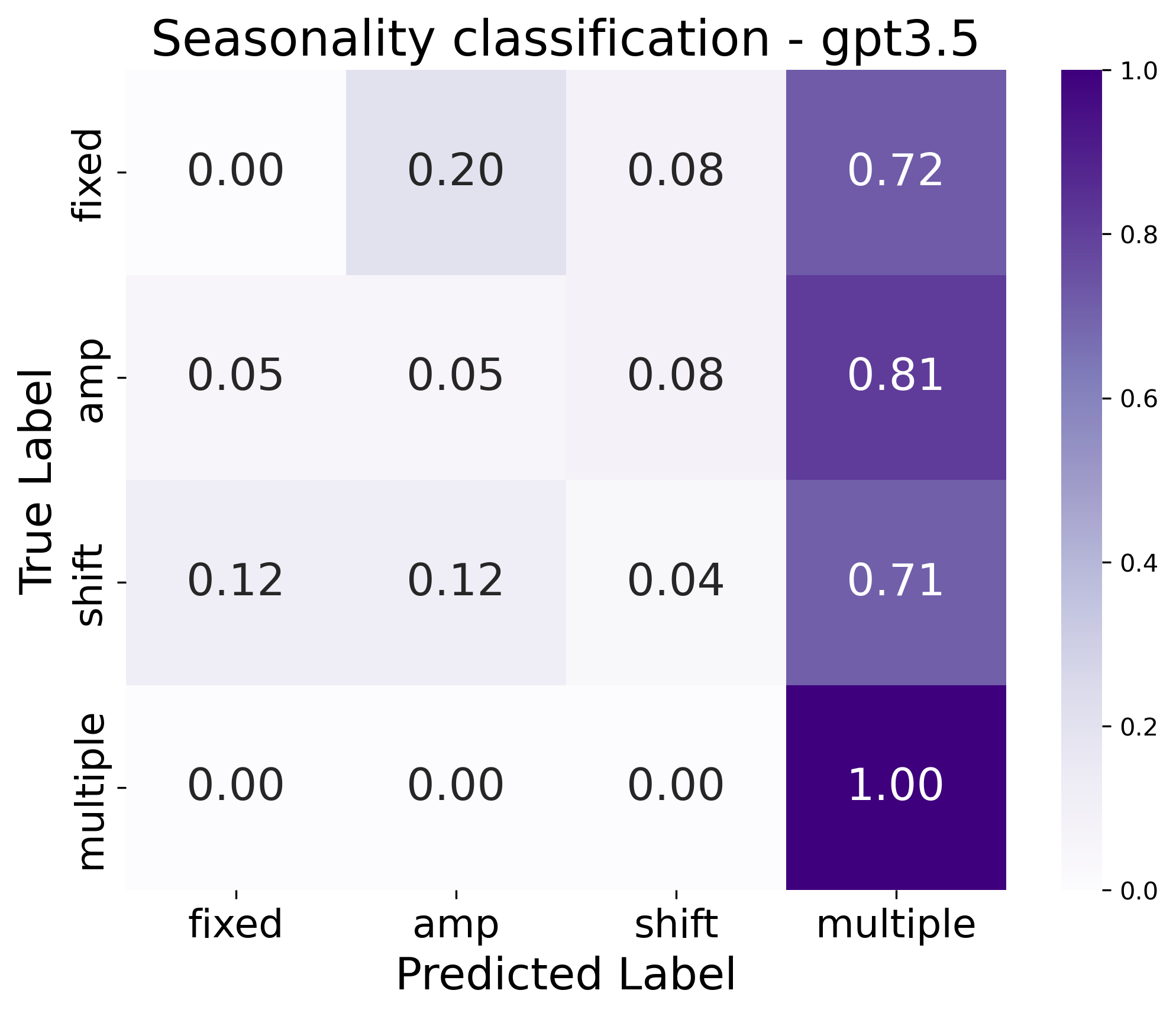
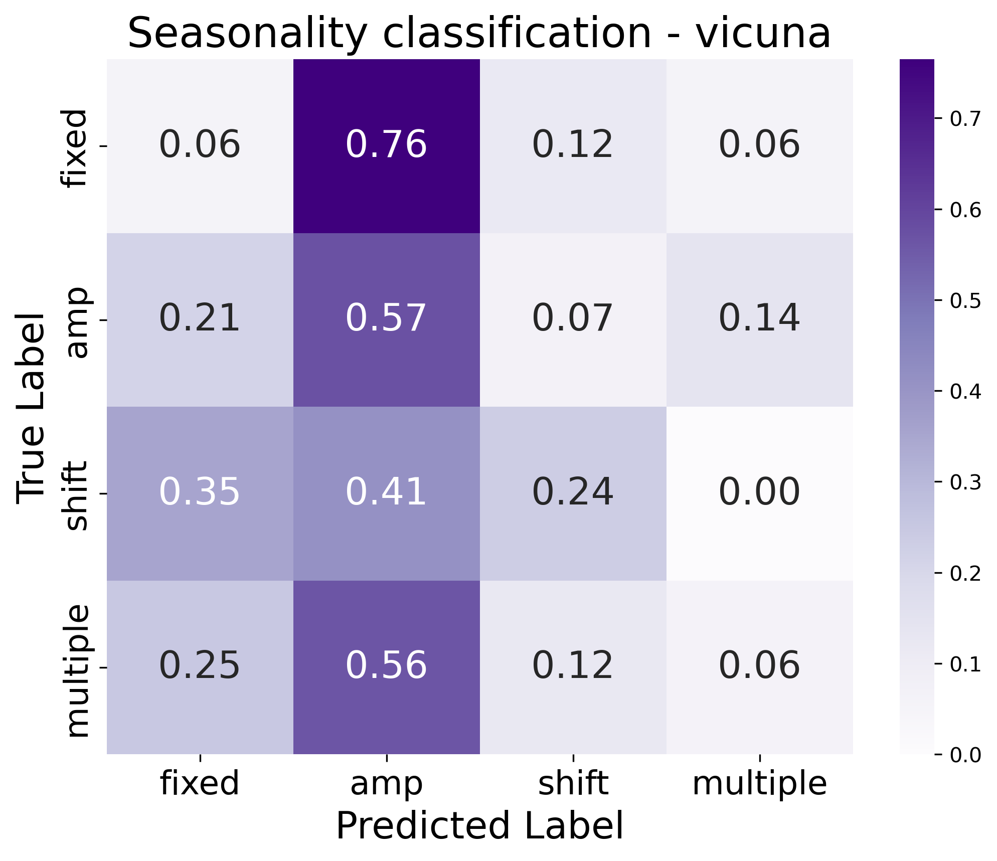
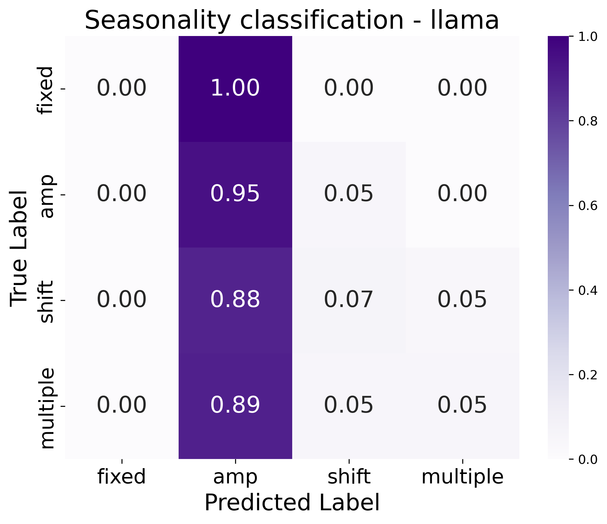
Figure 9: Seasonality classification

C.3 Anomalies

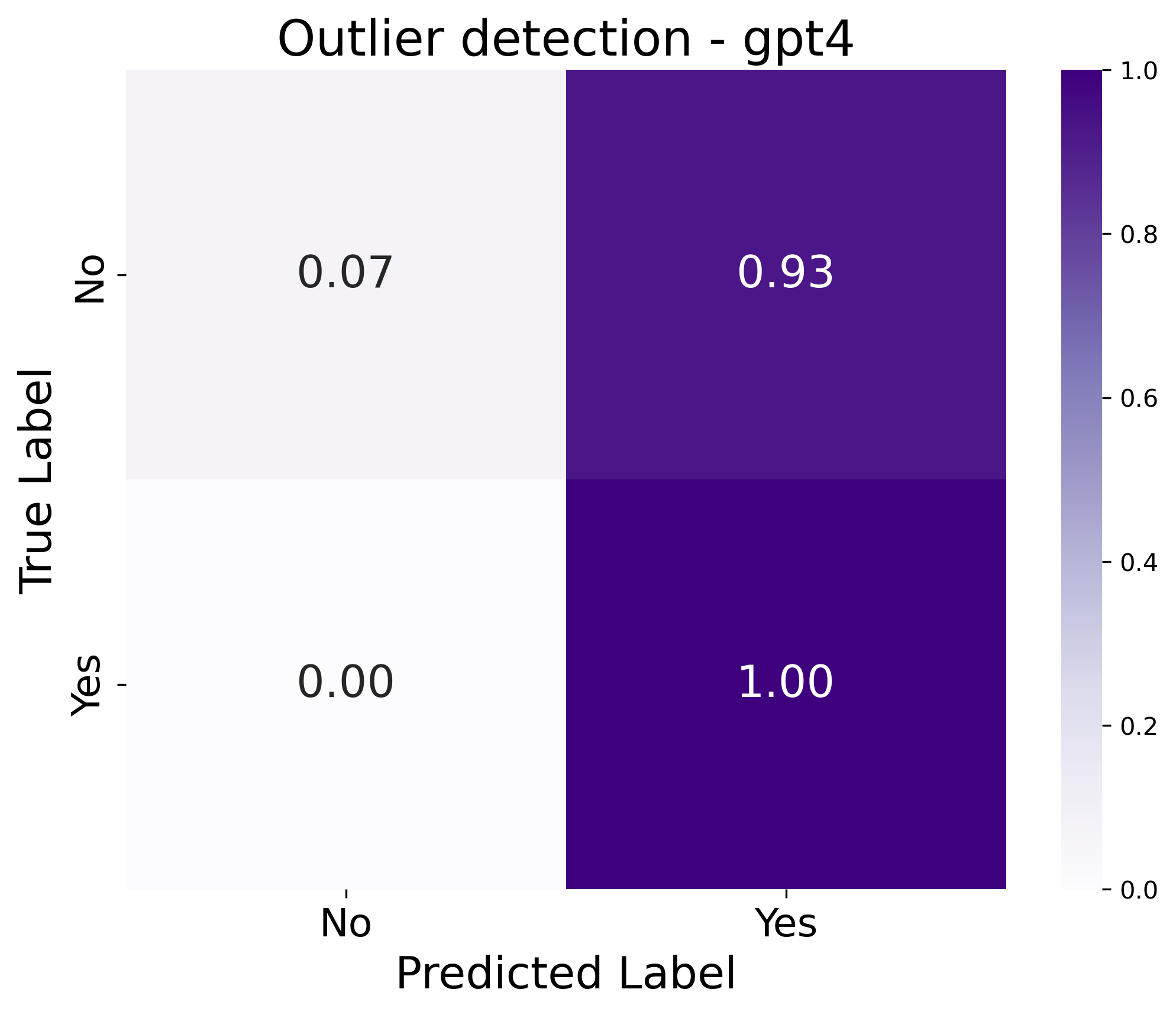
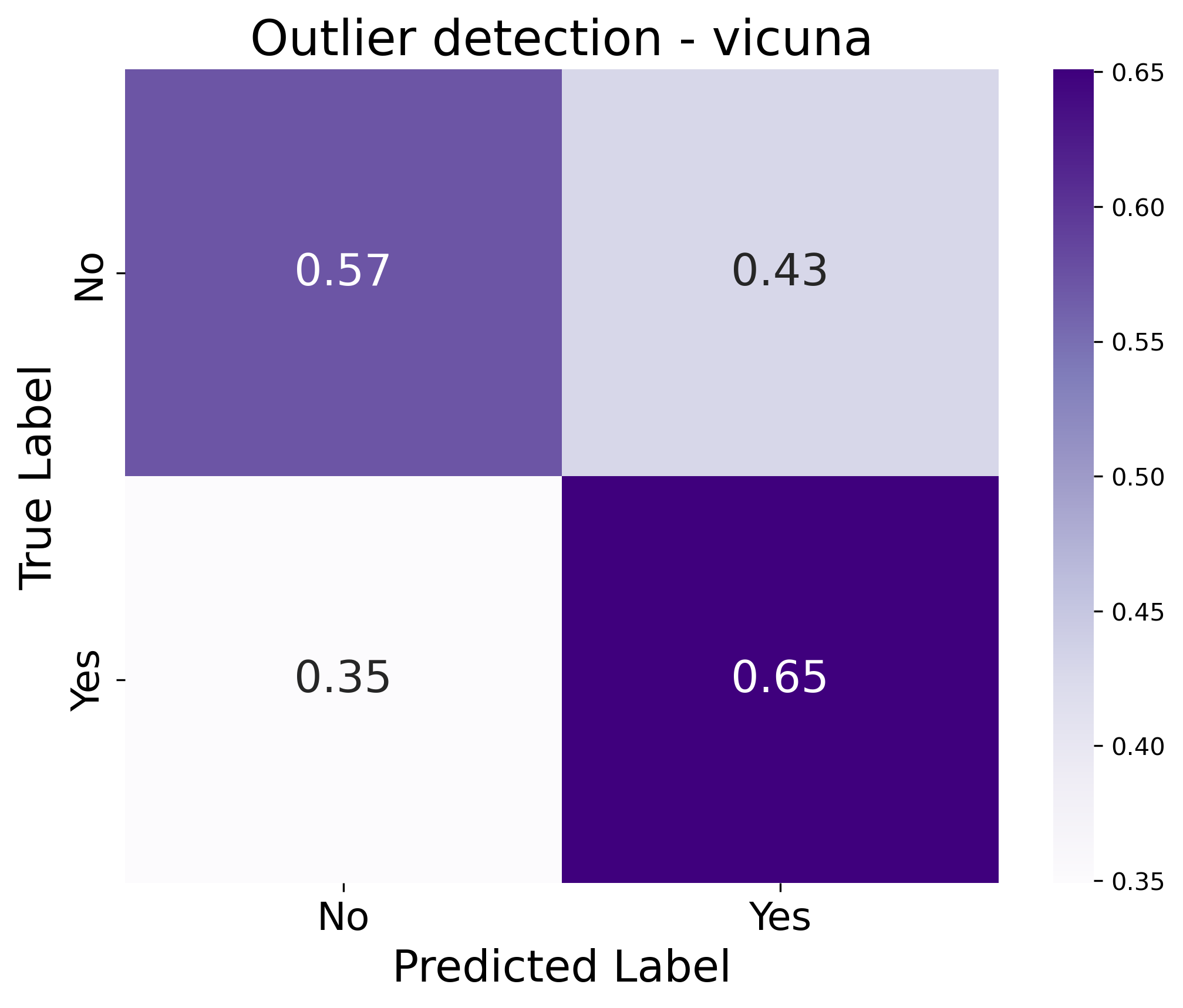
Figure 10: Anomaly detection

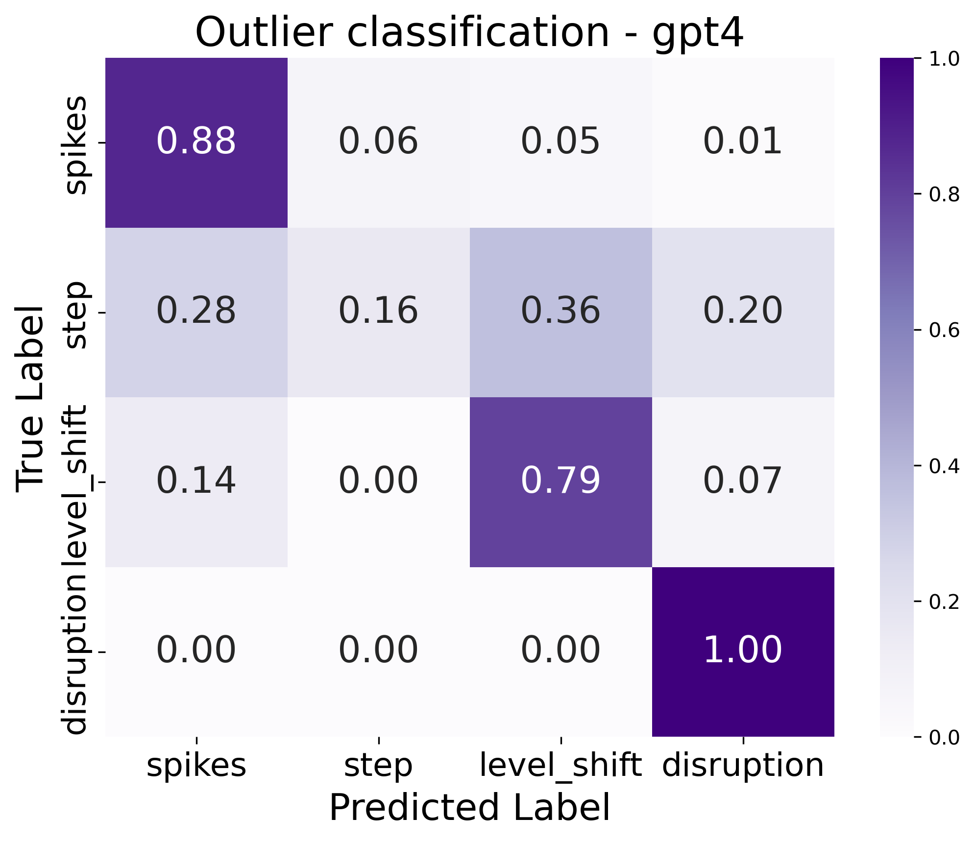
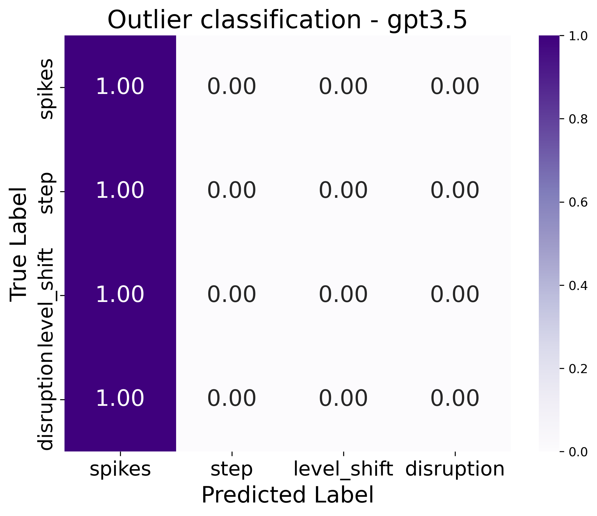
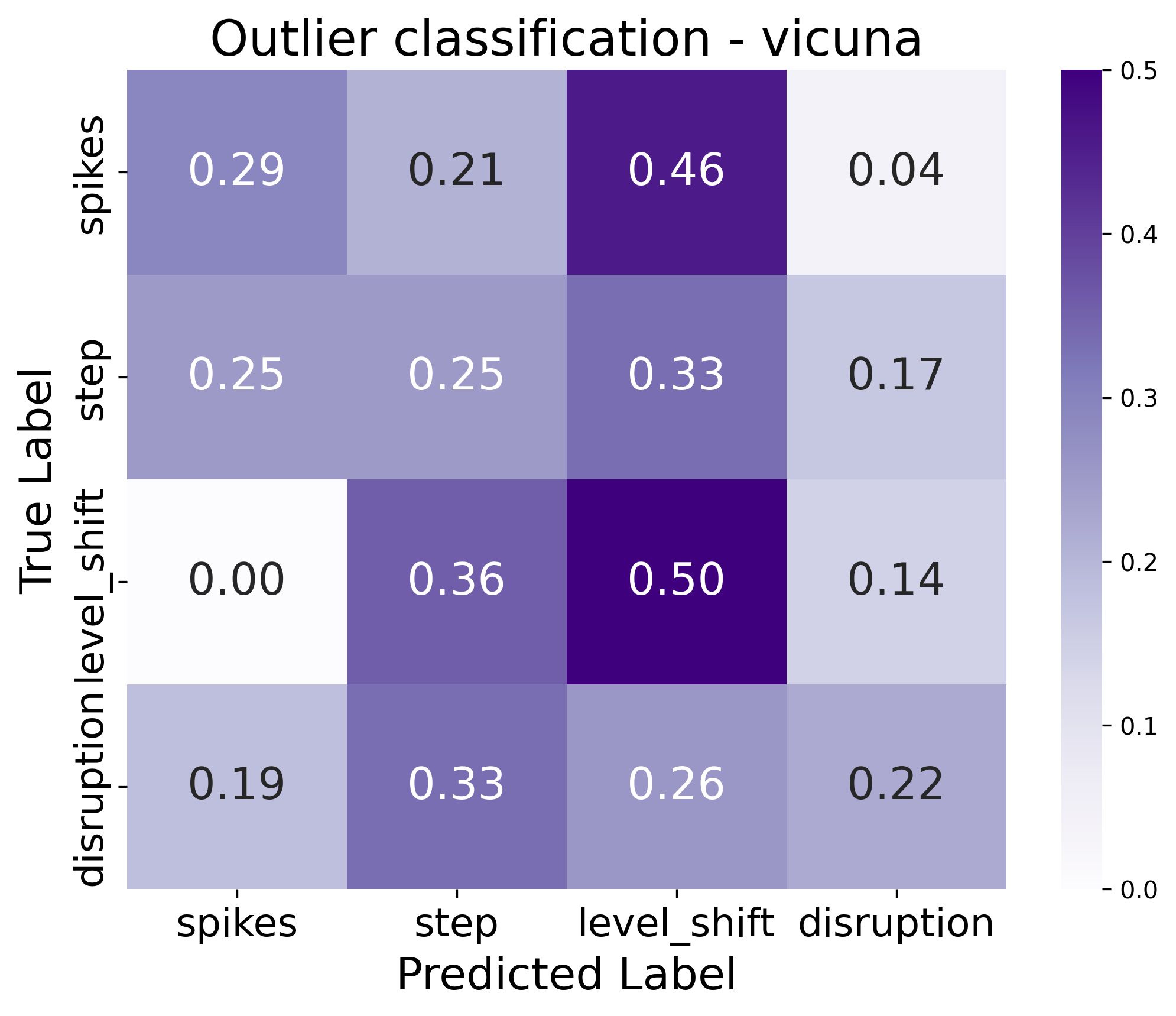
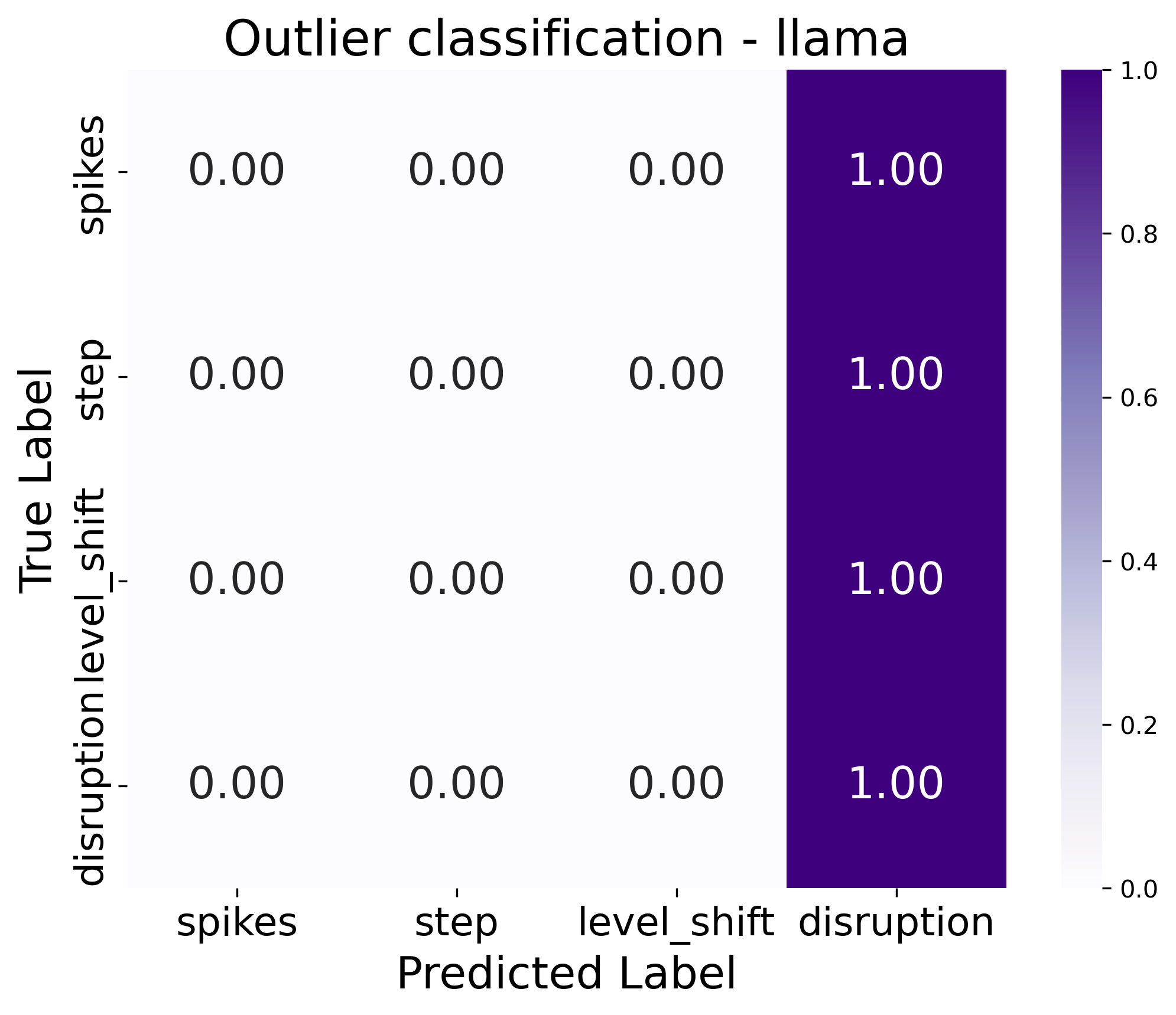
Figure 11: Anomaly classification

C.4 Volatility

Figure 12: Volatility detection

Figure 13: Volatility classification

Appendix D Position Bias

D.1 Does the position of the target value affect the performance of identifying its presence in various types of time series data?

Refer to Figure LABEL:fig:position_experiments_G0_search, which includes a confusion matrix (with ‘1: yes’ indicating presence of the number in the series and ‘0: no’ indicating its absence) and bar plot showing the accuracy in each quadrant for each LLM and type of time series data.

GPT achieves nearly perfect performance across all quadrants and time series types, indicating an absence of position bias in detecting the presence of a number within the time series. Llama2 does not exhibit position bias in monotonic series without noise but begins to show position bias as the complexity of the time series increases, such as in monotonic series with noise and sinusoidal series. We believe this bias is also present in Brownian series; however, due to the higher complexity of the dataset, Llama2’s performance is poor across all quadrants, making the impact of the bias less discernible. Vicuna displays superior performance compared to Llama2 across all datasets but continues to exhibit position bias. Notably, this bias appears in most datasets, such as monotonic series without noise, sinusoidal series, and Brownian motion series.

Table 6: Confusion matrix and accuracy by quadrant for the search task

GPT 3.5

(a) Monotonic (no noise) (b) Monotonic with noise (c) Sinusoidal (d) Brownian motion

Llama2

(a) Monotonic (no noise) (b) Monotonic with noise (c) Sinusoidal (d) Brownian motion

Vicuna

(a) Monotonic (no noise) (b) Monotonic with noise (c) Sinusoidal (d) Brownian motion

D.2 Does the position impact the retrieval performance for a specific date’s value from time series data?

Refer to Figure LABEL:fig:position_experiments_retrieval for bar plots that illustrate the accuracy across each quadrant.

Once again, GPT achieves nearly perfect performance across all quadrants and time series types, suggesting no position bias in the retrieval task either. Similar to the findings in D.1, Vicuna outperforms Llama2. Moreover, both Vicuna and Llama2 exhibit position bias in most datasets, including monotonic series both with and without noise, and sinusoidal series.

Table 7: Confusion matrix and accuracy by quadrant for the retrieval task

GPT 3.5

(a) Monotonic (no noise) (b) Monotonic with noise (c) Spikes (d) Brownian motion

Llama2

(a) Monotonic (no noise) (b) Monotonic with noise (c) Spikes (d) Brownian motion

Vicuna

(a) Monotonic (no noise) (b) Monotonic with noise (c) Spikes (d) Brownian motion

D.3 Does the position impact the efficiency of identifying minimum and maximum values in different types of time series data?

Refer to Figure LABEL:fig:position_experiments_min_max for bar charts illustrating the accuracy distribution across quadrants.

For the first time, GPT models show position bias in the spikes dataset, attributed to the increased complexity of the task, which involves arithmetic reasoning. Llama2 exhibits position bias in most datasets, notably in monotonic series with noise, spikes, and Brownian motion series. Vicuna also demonstrates position bias in most datasets, including monotonic series both with and without noise, as well as spikes series.

Table 8: Confusion matrix and accuracy by quadrant for the min-max extraction task. Note that monotonic series can have maximum or minimum values only in the first or fourth quadrant.

GPT 3.5

(a) Monotonic (no noise) (b) Monotonic with noise (c) Spikes (d) Brownian motion

Llama2

(a) Monotonic (no noise) (b) Monotonic with noise (c) Spikes (d) Brownian motion

Vicuna

(a) Monotonic (no noise) (b) Monotonic with noise (c) Spikes (d) Brownian motion

Appendix E Time Series formatting

Custom

⬇

"Date|Value\n2020-01-01|100\n2020-01-02|105\n2020-01-03|103\n2020-01-04|103\n"

⬇

Date|Value

2020-01-01|100

2020-01-02|105

2020-01-03|103

2020-01-04|103

TSV

⬇

"Date\tValue\n2020-01-01\t100\n2020-01-02\t105\n2020-01-03\t103\n2020-01-04\t103\n"

⬇

Date Value

2020-01-01 100

2020-01-02 105

2020-01-03 103

2020-01-04 103

Plain

⬇

"Date: 2020-01-01, Value: 100\nDate: 2020-01-02, Value: 105\nDate: 2020-01-03, Value: 103\nDate: 2020-01-04, Value: 103"

⬇

Date: 2020-01-01, Value: 100

Date: 2020-01-02, Value: 105

Date: 2020-01-03, Value: 103

Date: 2020-01-04, Value: 103

JSON

⬇

{"Date":"2020-01-01","Value":100}\n{"Date":"2020-01-02","Value":105}\n{"Date":"2020-01-03","Value":103}\n{"Date":"2020-01-04","Value":103}\n

⬇

{"Date":"2020-01-01","Value":100}

{"Date":"2020-01-02","Value":105}

{"Date":"2020-01-03","Value":103}

{"Date":"2020-01-04","Value":103}

Markdown

⬇

"|Date|Value|\n|---|---|\n|2020-01-01|100|\n|2020-01-02|105|\n|2020-01-03|103|\n|2020-01-04|103|\n"

⬇

|Date|Value|

|---|---|

|2020-01-01|100|

|2020-01-02|105|

|2020-01-03|103|

|2020-01-04|103|

Spaces

⬇

"Date,Value\n2020-01-01,1 0 0\n2020-01-02,1 0 5\n2020-01-03,1 0 3\n2020-01-04,1 0 3\n"

⬇

Date,Value

2020-01-01,1 0 0

2020-01-02,1 0 5

2020-01-03,1 0 3

2020-01-04,1 0 3

Context

⬇

"Date,Value\n2020-01-01,[100]\n2020-01-02,[105]\n2020-01-03,[103]\n2020-01-04,[103]\n"

⬇

Date,Value

2020-01-01,[100]

2020-01-02,[105]

2020-01-03,[103]

2020-01-04,[103]

Symbol

⬇

"Date,Value,DirectionIndicator\n2020-01-01,100,$\rightarrow$\n2020-01-02,105,$\uparrow$\n2020-01-03,103,$\downarrow$\n2020-01-04,103,$\rightarrow$\n"

⬇

Date,Value,DirectionIndicator

2020-01-01,100,$\rightarrow$

2020-01-02,105,$\uparrow$

2020-01-03,103,$\downarrow$

2020-01-04,103,$\rightarrow$

Base/csv

⬇

"Date,Value\n2020-01-01,100\n2020-01-02,105\n2020-01-03,103\n2020-01-04,103\n"

⬇

Date,Value

2020-01-01,100

2020-01-02,105

2020-01-03,103

2020-01-04,103

E.1 Additional results of time series formatting

(a) GPT3.5

	csv	plain	tsv	custom	contextual	json	markdown	spaces	symbol
Trend det	0.42	0.41	0.41	0.43	0.44	0.41	0.41	0.42	0.42
Trend class	0.74	0.55	0.72	0.61	0.85	0.50	0.56	0.53	0.92
Season det	0.61	0.77	0.69	0.60	0.58	0.87	0.44	0.63	0.47
Season class	0.27	0.19	0.21	0.16	0.23	0.22	0.09	0.17	0.18
Outlier det	0.55	0.52	0.50	0.49	0.46	0.49	0.48	0.52	0.62
Outlier class	0.17	0.17	0.17	0.16	0.17	0.17	0.17	0.17	0.17
AvgRank	3.33	5.75	4.00	6.08	4.50	5.25	7.25	4.83	4.00

(b) Llama2

	csv	plain	tsv	custom	contextual	json	markdown	spaces	symbol
Trend det	0.51	0.44	0.63	0.56	0.46	0.50	0.56	0.34	0.40
Trend class	0.41	0.48	0.40	0.43	0.45	0.42	0.36	0.43	0.62
Season det	0.55	0.24	0.48	0.46	0.59	0.38	0.45	0.40	0.50
Season class	0.11	0.13	0.09	0.10	0.09	0.10	0.11	0.08	0.10
Outlier det	0.44	0.35	0.47	0.44	0.45	0.48	0.51	0.41	0.47
Outlier class	0.13	0.14	0.10	0.14	0.17	0.18	0.21	0.14	0.08
AvgRank	4.83	5.50	5.33	4.33	4.33	4.83	3.83	7.17	4.83

(c) Vicuna

	csv	plain	tsv	custom	contextual	json	markdown	spaces	symbol
Trend det	0.51	0.49	0.47	0.47	0.55	0.44	0.51	0.54	0.45
Trend class	0.49	0.58	0.54	0.53	0.56	0.50	0.56	0.44	0.64
Season det	0.47	0.47	0.54	0.47	0.48	0.49	0.51	0.53	0.54
Season class	0.14	0.14	0.20	0.20	0.20	0.19	0.17	0.14	0.15
Outlier det	0.49	0.53	0.54	0.52	0.47	0.50	0.52	0.54	0.49
Outlier class	0.19	0.14	0.19	0.16	0.22	0.16	0.13	0.14	0.08
AvgRank	6.33	5.33	3.00	5.33	3.83	5.83	4.83	5.17	5.33

Table 9: Performance on Time Series Reasoning for different time series formatting.

(a) GPT3.5

	csv	plain	tsv	custom	contextual	json	markdown	spaces	symbol
Min value	0.98	0.99	0.98	0.98	0.98	0.98	0.98	0.79	0.98
Min date	0.94	0.95	0.94	0.95	0.94	0.94	0.93	0.69	0.93
Max value	0.92	0.92	0.91	0.92	0.92	0.91	0.91	0.54	0.94
Max date	0.88	0.88	0.88	0.88	0.88	0.86	0.86	0.51	0.89
Value on date	0.94	0.94	0.94	0.94	0.95	0.94	0.94	0.82	0.94
AvgRank	4.80	2.70	4.40	3.10	3.20	6.60	7.30	9.00	3.90

(b) Llama2

	csv	plain	tsv	custom	contextual	json	markdown	spaces	symbol
Min value	0.55	0.58	0.54	0.54	0.56	0.58	0.55	0.20	0.58
Min date	0.28	0.39	0.30	0.28	0.29	0.36	0.34	0.09	0.29
Max value	0.48	0.56	0.49	0.48	0.50	0.55	0.54	0.05	0.52
Max date	0.34	0.46	0.40	0.38	0.37	0.45	0.44	0.04	0.41
Value on date	0.39	0.38	0.47	0.40	0.35	0.45	0.44	0.07	0.34
AvgRank	6.80	2.30	4.60	6.50	5.60	2.10	3.50	9.00	4.60

(c) Vicuna

	csv	plain	tsv	custom	contextual	json	markdown	spaces	symbol
Min value	0.63	0.67	0.56	0.61	0.60	0.64	0.59	0.17	0.62
Min date	0.50	0.55	0.47	0.49	0.53	0.52	0.51	0.13	0.49
Max value	0.49	0.46	0.45	0.44	0.48	0.47	0.50	0.01	0.50
Max date	0.38	0.42	0.41	0.39	0.46	0.40	0.42	0.07	0.41
Value on date	0.36	0.48	0.39	0.39	0.42	0.40	0.37	0.09	0.41
AvgRank	5.40	2.40	6.50	6.60	3.00	4.00	4.30	9.00	3.80

Table 10: Accuracy for information retrieval and arithmetic reasoning tasks for different time series formatting.

(a) GPT3.5

	csv	plain	tsv	custom	contextual	json	markdown	spaces	symbol
Min value	0.04	0.04	0.05	0.04	0.04	0.06	0.07	0.32	0.04
Max value	0.06	0.07	0.07	0.07	0.07	0.10	0.09	1.01	0.10
Value on date	0.08	0.10	0.07	0.08	0.03	0.08	0.03	0.38	0.04

(b) Llama2

	csv	plain	tsv	custom	contextual	json	markdown	spaces	symbol
Min value	10.15	16.18	10.38	19.57	22.46	11.14	21.15	0.69	21.12
Max value	1.03	0.95	1.09	1.04	0.91	1.01	1.00	2.58	0.90
Value on date	0.81	0.65	0.40	0.73	0.61	0.48	0.44	0.96	0.90

(c) Vicuna

	csv	plain	tsv	custom	contextual	json	markdown	spaces	symbol
Min value	12.79	12.24	29.45	13.89	12.06	26.62	25.54	0.96	22.50
Max value	0.85	0.74	1.01	1.14	0.94	0.67	0.98	2.51	0.59
Value on date	0.44	0.78	0.83	0.94	0.31	0.65	0.38	0.95	0.38

Table 11: MAPE for information retrieval and arithmetic reasoning tasks for different time series formatting.

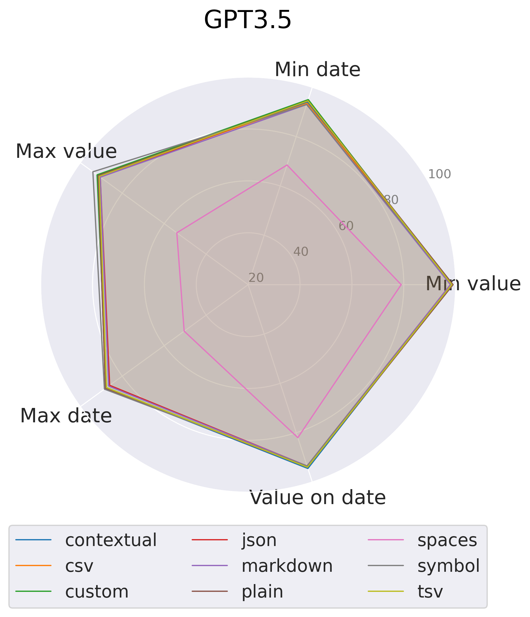
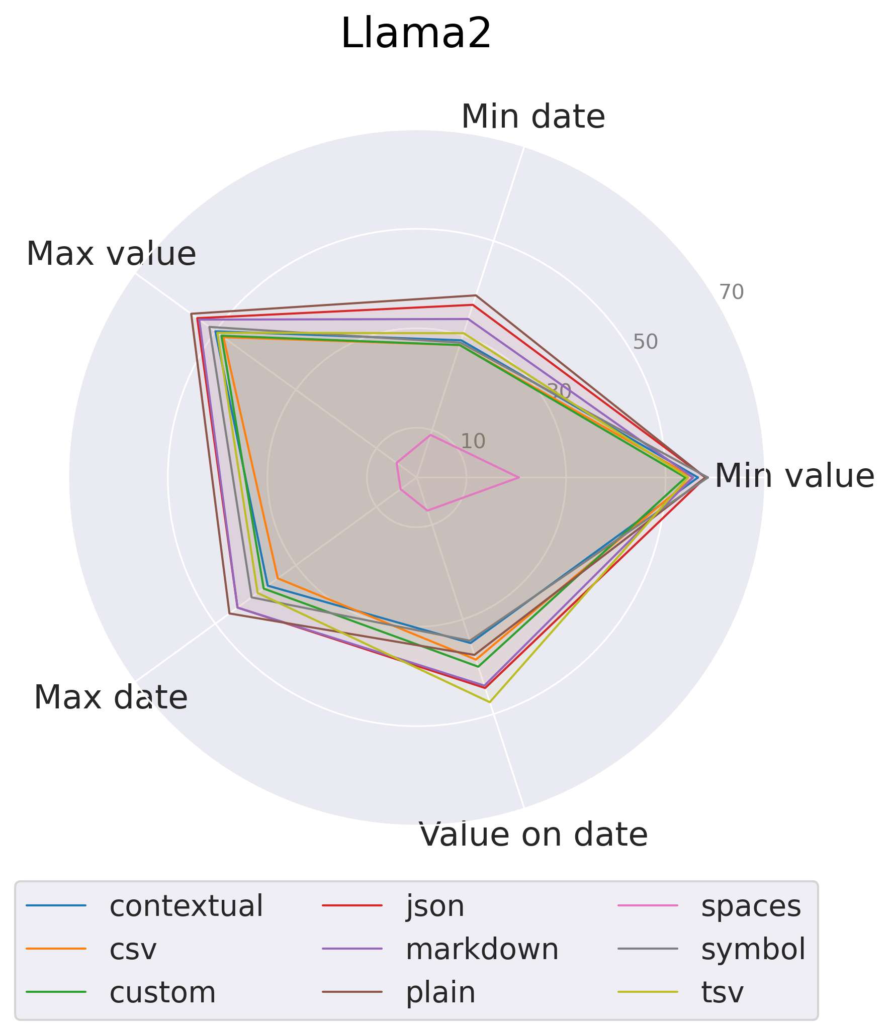
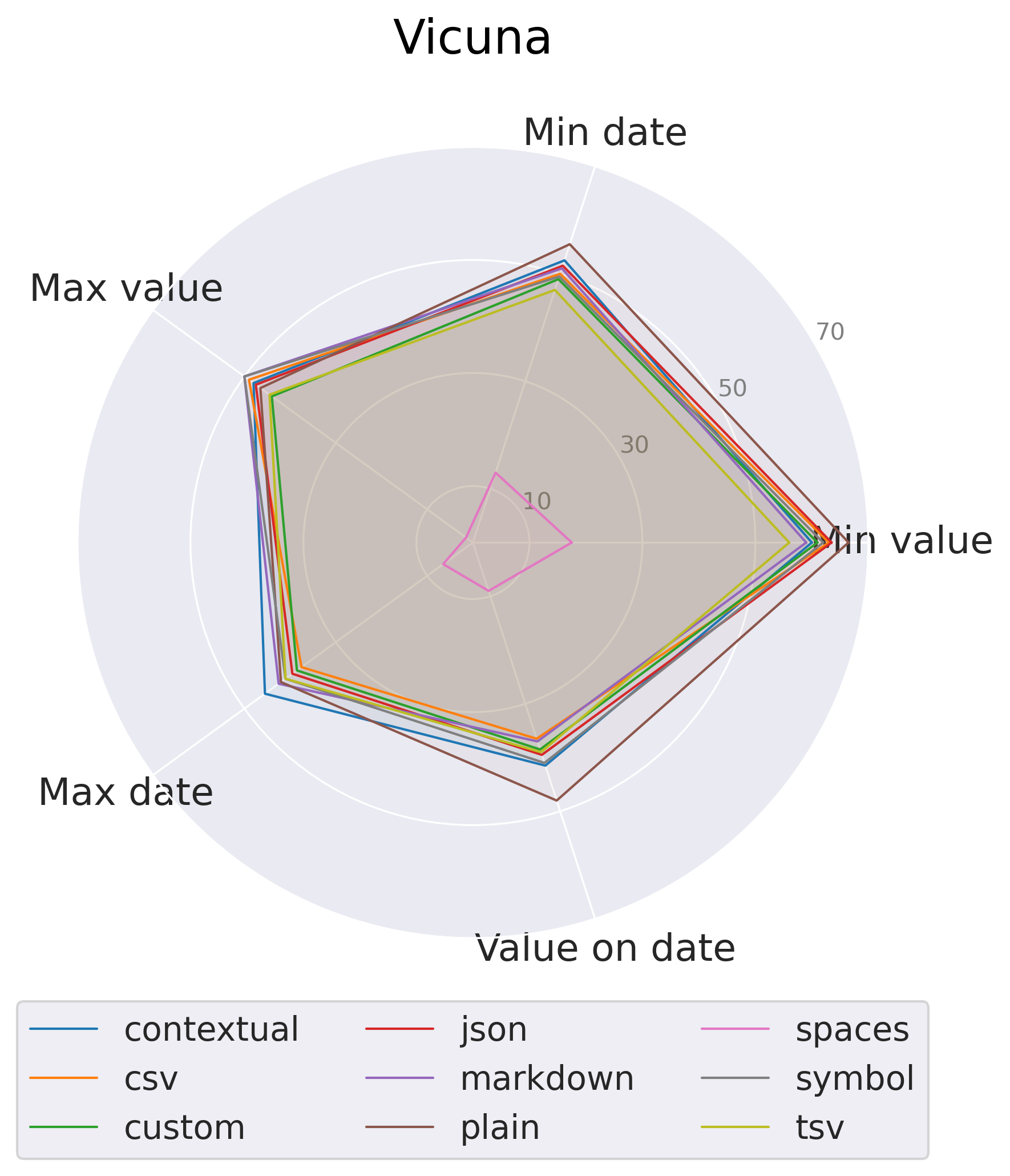
Figure 14: Accuracy for information retrieval and arithmetic reasoning tasks for different time series tokenization.

Appendix F Prompts

Appendix G Licenses

Table 12 lists the licenses for the assets used in the paper.

Asset	License
Llama2	Link
Vicuna1.5	Link

Table 12: License of assets used.

References

- Achiam et al. (2023) Josh Achiam, Steven Adler, Sandhini Agarwal, Lama Ahmad, Ilge Akkaya, Florencia Leoni Aleman, Diogo Almeida, Janko Altenschmidt, Sam Altman, Shyamal Anadkat, et al. 2023. Gpt-4 technical report. arXiv preprint arXiv:2303.08774.
- Azerbayev et al. (2023) Zhangir Azerbayev, Hailey Schoelkopf, Keiran Paster, Marco Dos Santos, Stephen McAleer, Albert Q. Jiang, Jia Deng, Stella Biderman, and Sean Welleck. 2023. Llemma: An open language model for mathematics.
- Brown et al. (2020) Tom Brown, Benjamin Mann, Nick Ryder, Melanie Subbiah, Jared D Kaplan, Prafulla Dhariwal, Arvind Neelakantan, Pranav Shyam, Girish Sastry, Amanda Askell, et al. 2020. Language models are few-shot learners. Advances in neural information processing systems, 33:1877–1901.
- Chen et al. (2023) Shengchao Chen, Guodong Long, Jing Jiang, Dikai Liu, and Chengqi Zhang. 2023. Foundation models for weather and climate data understanding: A comprehensive survey. arXiv preprint arXiv:2312.03014.
- Chen et al. (2024) Yuqi Chen, Kan Ren, Kaitao Song, Yansen Wang, Yifan Wang, Dongsheng Li, and Lili Qiu. 2024. Eegformer: Towards transferable and interpretable large-scale eeg foundation model.
- Chiang et al. (2023) Wei-Lin Chiang, Zhuohan Li, Zi Lin, Ying Sheng, Zhanghao Wu, Hao Zhang, Lianmin Zheng, Siyuan Zhuang, Yonghao Zhuang, Joseph E. Gonzalez, Ion Stoica, and Eric P. Xing. 2023. Vicuna: An open-source chatbot impressing gpt-4 with 90%* chatgpt quality.
- Chowdhery et al. (2023) Aakanksha Chowdhery, Sharan Narang, Jacob Devlin, Maarten Bosma, Gaurav Mishra, Adam Roberts, Paul Barham, Hyung Won Chung, Charles Sutton, Sebastian Gehrmann, et al. 2023. Palm: Scaling language modeling with pathways. Journal of Machine Learning Research, 24(240):1–113.
- Gruver et al. (2023) Nate Gruver, Marc Finzi, Shikai Qiu, and Andrew Gordon Wilson. 2023. Large language models are zero-shot time series forecasters.
- Jiang et al. (2024) Yushan Jiang, Zijie Pan, Xikun Zhang, Sahil Garg, Anderson Schneider, Yuriy Nevmyvaka, and Dongjin Song. 2024. Empowering time series analysis with large language models: A survey. ArXiv, abs/2402.03182.
- Kim et al. (2021) Jeonghwan Kim, Giwon Hong, Kyung min Kim, Junmo Kang, and Sung-Hyon Myaeng. 2021. Have you seen that number? investigating extrapolation in question answering models. In Conference on Empirical Methods in Natural Language Processing.
- Liu and Low (2023) Tiedong Liu and Bryan Kian Hsiang Low. 2023. Goat: Fine-tuned llama outperforms gpt-4 on arithmetic tasks.
- Nogueira et al. (2021) Rodrigo Nogueira, Zhiying Jiang, and Jimmy Lin. 2021. Investigating the limitations of transformers with simple arithmetic tasks.
- Qiu et al. (2023) Jielin Qiu, William Han, Jiacheng Zhu, Mengdi Xu, Michael Rosenberg, Emerson Liu, Douglas Weber, and Ding Zhao. 2023. Transfer knowledge from natural language to electrocardiography: Can we detect cardiovascular disease through language models?
- Touvron et al. (2023) Hugo Touvron, Louis Martin, Kevin Stone, Peter Albert, Amjad Almahairi, Yasmine Babaei, Nikolay Bashlykov, Soumya Batra, Prajjwal Bhargava, Shruti Bhosale, Dan Bikel, Lukas Blecher, Cristian Canton Ferrer, Moya Chen, Guillem Cucurull, David Esiobu, Jude Fernandes, Jeremy Fu, Wenyin Fu, Brian Fuller, Cynthia Gao, Vedanuj Goswami, Naman Goyal, Anthony Hartshorn, Saghar Hosseini, Rui Hou, Hakan Inan, Marcin Kardas, Viktor Kerkez, Madian Khabsa, Isabel Kloumann, Artem Korenev, Punit Singh Koura, Marie-Anne Lachaux, Thibaut Lavril, Jenya Lee, Diana Liskovich, Yinghai Lu, Yuning Mao, Xavier Martinet, Todor Mihaylov, Pushkar Mishra, Igor Molybog, Yixin Nie, Andrew Poulton, Jeremy Reizenstein, Rashi Rungta, Kalyan Saladi, Alan Schelten, Ruan Silva, Eric Michael Smith, Ranjan Subramanian, Xiaoqing Ellen Tan, Binh Tang, Ross Taylor, Adina Williams, Jian Xiang Kuan, Puxin Xu, Zheng Yan, Iliyan Zarov, Yuchen Zhang, Angela Fan, Melanie Kambadur, Sharan Narang, Aurelien Rodriguez, Robert Stojnic, Sergey Edunov, and Thomas Scialom. 2023. Llama 2: Open foundation and fine-tuned chat models.
- Vaswani et al. (2017) Ashish Vaswani, Noam Shazeer, Niki Parmar, Jakob Uszkoreit, Llion Jones, Aidan N Gomez, Ł ukasz Kaiser, and Illia Polosukhin. 2017. Attention is all you need. In Advances in Neural Information Processing Systems, volume 30. Curran Associates, Inc.
- Wang et al. (2024) Xinglei Wang, Meng Fang, Zichao Zeng, and Tao Cheng. 2024. Where would i go next? large language models as human mobility predictors.
- Xue and Salim (2023) Hao Xue and Flora D. Salim. 2023. Promptcast: A new prompt-based learning paradigm for time series forecasting. IEEE Transactions on Knowledge and Data Engineering, pages 1–14.
- Yu et al. (2023) Xinli Yu, Zheng Chen, Yuan Ling, Shujing Dong, Zongying Liu, and Yanbin Lu. 2023. Temporal data meets llm - explainable financial time series forecasting. ArXiv, abs/2306.11025.
- Yuan et al. (2023) Zheng Yuan, Hongyi Yuan, Chuanqi Tan, Wei Wang, and Songfang Huang. 2023. How well do large language models perform in arithmetic tasks?
- Zhang et al. (2024) Xiyuan Zhang, Ranak Roy Chowdhury, Rajesh K. Gupta, and Jingbo Shang. 2024. Large language models for time series: A survey. ArXiv, abs/2402.01801.
- Zhao et al. (2023) Wayne Xin Zhao, Kun Zhou, Junyi Li, Tianyi Tang, Xiaolei Wang, Yupeng Hou, Yingqian Min, Beichen Zhang, Junjie Zhang, Zican Dong, et al. 2023. A survey of large language models. arXiv preprint arXiv:2303.18223.
- Zhao et al. (2021) Zihao Zhao, Eric Wallace, Shi Feng, Dan Klein, and Sameer Singh. 2021. Calibrate before use: Improving few-shot performance of language models. In International Conference on Machine Learning, pages 12697–12706. PMLR.
- Zhou et al. (2023) Tian Zhou, Peisong Niu, Xue Wang, Liang Sun, and Rong Jin. 2023. One fits all: Power general time series analysis by pretrained lm. arXiv preprint arXiv:2302.11939.