Conductivity of lattice bosons at high temperatures
Abstract
Quantum simulations are quickly becoming an indispensable tool for studying particle transport in correlated lattice models. One of the central topics in the study of transport is the bad-metal behavior, characterized by the direct current (dc) resistivity linear in temperature. In the fermionic Hubbard model, optical conductivity has been studied extensively, and a recent optical lattice experiment has demonstrated bad metal behavior in qualitative agreement with theory. Far less is known about transport in the bosonic Hubbard model. We investigate the conductivity in the Bose-Hubbard model, and focus on the regime of strong interactions and high-temperatures. We use numerically exact calculations for small lattice sizes. At weak tunneling, we find multiple peaks in the optical conductivity that stem from the Hubbard bands present in the many-body spectrum. This feature slowly washes out as the tunneling rate gets stronger. At high temperature, we identify a regime of -linear resistivity, as expected. When the interactions are very strong, the leading inverse-temperature coefficient in conductivity is proportional to the tunneling amplitude. As the tunneling becomes stronger, this dependence takes quadratic form. At very strong coupling and half filling, we identify a separate linear resistivity regime at lower temperature, corresponding to the hard-core boson regime. Additionally, we unexpectedly observe that at half filling, in a big part of the phase diagram, conductivity is an increasing function of the coupling constant before it saturates at the hard-core-boson result. We explain this feature based on the analysis of the many-body energy spectrum and the contributions to conductivity of individual eigenstates of the system.
I Introduction
Cold atoms in optical lattices have provided a clean and tunable realization of the Hubbard model Bloch et al. (2008). The focus of early experiments was on studying phase transitions within the model, but various aspects of nonequilibrium dynamics have also been explored in this setup. In particular, a lot of effort is invested in performing transport measurements with cold atoms Chien et al. (2015); Krinner et al. (2017); Brown et al. (2019). Transport measurements in optical lattices are of great interest as they allow to isolate the effects of strong correlations from the effects of phonons and disorder, in a way that is not possible in real materials.
Particular attention is paid to linear-in-temperature resistivity, which is believed to be related to the superconducting phase and/or quantum critical points in the cuprates and more general strongly correlated systemsGrigera et al. (2001); Cooper et al. (2009); Cao et al. (2018); Legros et al. (2018); Licciardello et al. (2019); Cha et al. (2020). This phenomenon has been studied theoretically in different versions of the Fermi-Hubbard model and in different parameter regimesDeng et al. (2013); Vučičević et al. (2015); Perepelitsky et al. (2016); Vučičević et al. (2019); Vranić et al. (2020); Kiely and Mueller (2021); Vučičević et al. (2023). The onset of resistivity linear in temperature has been addressed in more general terms from the theoretical side in Refs. Mukerjee et al. (2006); Herman et al. (2019); Patel and Changlani (2022). In experiment with fermionic cold atoms in optical lattices, the -linear resistivity has also been observed to span a large range of temperature, in qualitative agreement with theoryBrown et al. (2019). However, the transport in bosonic lattice models has been less studied, from both theoretical and experimental perspectives.
Bosonic transport in the strongly interacting regime of the Bose-Hubbard model has been addressed in a cold-atom setup by investigating expansion dynamics induced by a harmonic-trap removal Vidmar et al. (2013); Ronzheimer et al. (2013) and by studying center-of-mass oscillations induced by a trap displacement Snoek and Hofstetter (2007); Dhar et al. (2019). However these studies do not focus on optical conductivity. Optical conductivity of bosons at zero and low temperature has been calculated in early papers Fisher et al. (1989); Cha et al. (1991); Kampf and Zimanyi (1993). Conductivity of two-dimensional hard-core bosons has been addressed in Refs. Lindner and Auerbach (2010); Bhattacharyya et al. (2023) and a large temperature range with linearly increasing resistivity has been found. Conductivity of strongly correlated bosons in optical lattices in a synthetic magnetic field was obtained in Ref. Sajna et al. (2014). The regime of resistivity linear temperature has been recently investigated for the Bose-Hubbard model at weak coupling Rizzatti and Mueller (2023). Dynamical response within the scaling regime of the quantum critical point and universal conductivity at the quantum phase transition have been investigated theoretically in an attempt to establish a clear connection with ADS-CFT mapping Chen et al. (2014); Lucas et al. (2017). In addition to cold atom studies, bosonic transport properties have been studied in the context of an emergent Bose liquid Zeng et al. (2021); Hegg et al. (2021); Yue et al. (2023). Transport properties of a nanopatterned YBCO film arrays have been analyzed in terms of bosonic strange metal featuring resistivity linear in temperature down to low temperatures Yang et al. (2022).
In this paper, we study conductivity in the Bose-Hubbard modelFisher et al. (1989); Bloch et al. (2008) as relevant for optical lattice experiments with bosonic atoms. We consider strongly-interacting regime and focus on high temperatures, away from any ordering instabilities. We consider small lattice sizes of up to lattice sites, and employ averaging over twisted boundary conditions to lessen the finite-size effects. We control our results by comparing different lattice sizes, as well as by checking sum rules to make sure that charge stiffness is negligible. We also use both the canonical and grand canonical ensemble, and compare results. To solve the model, we use exact diagonalization and finite-temperature Lanczos methodPrelovšek and Bonča (2013).
We compute and analyze the probability distribution of the eigenenergies (the many-body density of states), the spectral function, the optical and the dc conductivity, as well as some thermodynamic quantities. Where applicable, we compare results to the hard-core limit, the classical limit as well as to the results obtained by the bubble-diagram approximation. Our results show several expected features. First, the many-body density of states, spectral function and the optical conductivity, all simultaneously develop gaps and the corresponding Hubbard bands as the coupling is increased. Next, we clearly identify the linear dc resistivity regime at high temperature, and find the connection of the slope with the tunneling amplitude, along the lines of Ref. Patel and Changlani (2022). Furthermore, at lower temperatures and high coupling, we identify a separate linear resistivity regime corresponding to hard-core-like behavior, which can be expected on general grounds. We also find some unexpected features: we observe non-monotonic behavior in the dc conductivity as a function of the coupling constant, which we map out throughout the phase diagram.
The paper is organized as follows: In Sec. II, we briefly describe our method of choice. In Sec. III we present our results: in subsection III.1 we address the many-body density of states and in subsection III.2 we show some thermodynamic properties of the Bose-Hubbard model in the high-temperature regime. In subsection III.3 we calculate optical conductivity for a finite interaction strength and in subsection III.4 we investigate the dependence of the direct-current conductivity on microscopic parameters of the Bose-Hubbard model and temperature. In subsection III.5 we explain observed features using an analysis of the Kubo formula from Ref. Patel and Changlani (2022). Then in subsection III.6 we compare our results for half filling with the results for hard-core bosons Lindner and Auerbach (2010). We discuss finite-size effects in subsection III.7 and compare results obtained within the canonical ensemble with the results obtained within the grand-canonical ensemble in subsection III.8. In subsection III.9 we compare our results obtained for small lattices with the result of often used bubble-diagram approximation. Finally, we summarize our findings in Sec. IV.
II Model and Methods
Cold bosonic atoms in optical lattices are realistically described by the Bose-Hubbard model Bloch et al. (2008)
| (1) |
where is the tunneling amplitude between nearest-neighbor sites of a square lattice and is the on-site density-density interaction. Unless stated differently, our units are set by the choice . Throughout the paper, we set lattice constant , , . We also assume that effective charge of particles is .
The quantitative finite-temperature phase diagram of the model on a square lattice was obtained in Ref. Capogrosso-Sansone et al. (2008). At integer filling, a quantum phase transition between a Mott insulator state and a superfluid is found (in particular, for filling boson per site, the transition occurs at . At finite temperature a BKT transition describes the loss of superfluidity Prokof’ev et al. (2001). In this paper we work in the high-temperature regime where we expect only normal (non-condensed) state and short-range correlations.
We consider the retarded current-current correlation function at finite temperature
| (2) |
where the current operator is given by
| (3) |
with the summation only over nearest-neighbors along direction. The partition function is and averaging is performed as
| (4) |
In the linear response regime, the conductivity is given by the Kubo formulaMahan (2000); Scalapino et al. (1992)
| (5) |
where and is the average kinetic energy along direction. Note that for the real conductivity from Eq. (5), we need imaginary part of the correlation function . The direct-current (DC) conductivity is obtained as .
In the following we rely on numerically exact approaches for small lattice sizes. We use exact diagonalization to obtain the eigenenergies and eigenstates of the Hamiltonian and calculate
| (6) | |||||
For larger lattice sizes, we apply the finite-temperature Lanczos method Prelovšek and Bonča (2013). We employ averaging over twisted boundary conditions to lessen the finite-size effects Poilblanc (1991); Gros (1992).
Due to the expected onset of charge stiffness in finite systems and, more generally, longer range correlations at low temperature, we expect our method to be limited to the regime of high temperature and relatively strong interactions (corresponding to a smaller ratio ). For a crosscheck of the validity of our numerical approaches, we rely on the comparison of different lattice sizes (subsection III.7) and the sum rule
| (7) |
Indeed, we find that the sum rule is satisfied at temperatures and tunneling . In this regime we find that the results no longer significantly change with increasing lattice size (subsection III.7), thus our results are expected to be reasonably representative of the thermodynamic limit.
Finally, we control the results with respect to the choice of the statistical ensemble. A comparison of the results obtained with the grand-canonical and canonical ensembles is given in Sec. III.8. We do not find substantial difference in the results between the two statistical ensembles, thus we choose to work in the canonical ensemble, as it allows us to consider larger lattices. Unless stated differently, the results presented in the paper are for the canonical ensemble.
III Results
III.1 Eigenstate spectrum
We first consider the many-body density of states of the model (1) defined by
| (8) |
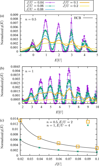
We show our numerical results for fillings and in Fig. 1(a).
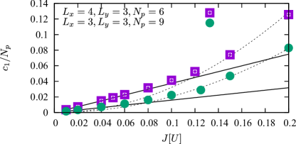
The classical limit is simple to understand. The many-body spectrum features energies with huge degeneracies. The Hilbert space dimension is , where is the number of lattice sites, and is the number of particles. For , there are states with zero energy, the states (a single-site occupied with two bosons) with energy , and so on. The number of different energy levels is set by the system size that we consider. As the ratio increases from zero, these macroscopic degeneracies are slowly resolved, and the bands obtain a finite width. This is precisely what we observe in the numerical data, as shown in Fig. 1(a), but we find that separate many-body bands do persist up to a finite value of , regardless of filling. Around this value, the peaks in (found around ) have heights roughly proportional to , see Fig. 1(c). As increases further, the density of states turns into a wide, bell-shaped curve, as shown in Fig. 1(b) for unit filling at . This particular feature of the spectrum has been considered for a related one-dimensional model in Ref. Kollath et al. (2010). We also observe that for , the lowest many-body band can be reasonably approximated by hard-core bosons.
III.2 Thermodynamic properties
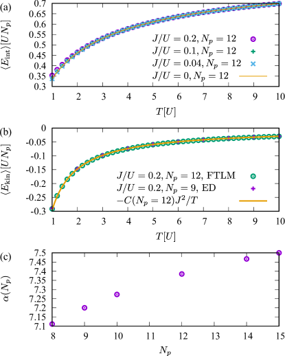
We investigate thermodynamical properties for , as this regime has not been discussed in much detail in literature. Interaction energy
| (9) |
is very weakly dependent on the tunneling as shown in Fig. 2(a), for the tunneling range that we consider . The average value of the kinetic energy
| (10) |
can be reasonably approximated by the leading order in the high-temperature expansion
| (11) | |||||
| (12) | |||||
| (13) | |||||
| (14) |
where is the number of particles in the system and is the dimension of the Hilbert space. The coefficient is size dependent, see Fig. 2(c).
III.3 Optical conductivity
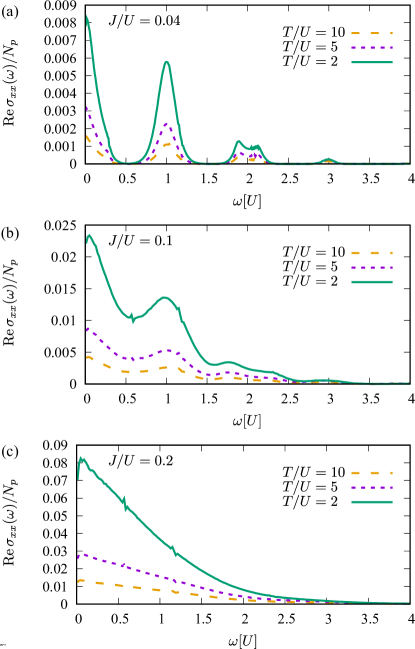
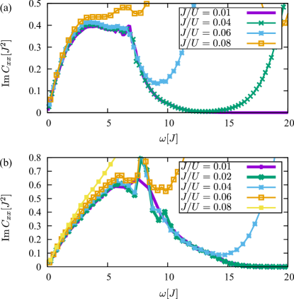
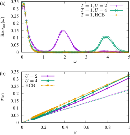
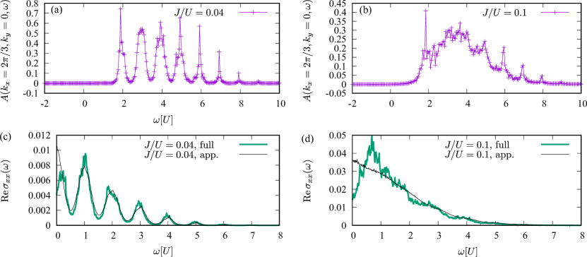
We present numerical results for the optical conductivity in Fig. 3 for bosons with and temperatures . We check that within this range of physical parameters the sum rule given in Eq. (7) is satisfied with accuracy better than one percent. For the weak tunneling amplitudes we observe that the conductivity exhibits multiple peaks at that stem from the energy bands of the Hubbard model, as shown in Fig. 1. As temperature is lowered, the higher-energy peaks become smaller relative to the low-energy peaks, which is clearly expected. However, in absolute terms, the optical conductivity gets smaller with increasing temperature, at all frequencies. As the tunneling gets stronger the peaks merge, but the multi-peak structure is still visible at intermediate hopping . Finally for the conductivity takes a simpler form, see Fig. 3 (c). In Fig. (4) we show that at low frequency, the current-current correlation function scales with temperature in a simple way, but the behavior is more complicated at higher frequencies.
III.4 DC limit and -linear resistivity
We now focus on the range of small . We have seen that the strong interaction introduces gaps in the many-body spectrum that translate into peaks in the optical conductivity. In order to address the role of tunneling in more detail, we replot numerical data in Fig. 5 by showing the current-current correlation as a function of . The rescaling by is motivated by the basic definition of the current-current correlation function from Eq. (2). We find that for up to numerical data overlap near and are very weakly dependent on . We further analyze and explain this feature in Sec. III.5.
In order to extract the DC conductivity from the current-current correlation function, we consider small but finite and perform a linear fit . For numerical purposes we perform the fitting in the range .
In Fig. 6 we plot DC conductivity as a function of inverse temperature . Overall, we find that the normalized conductivity decreases with filling from to in this strongly interacting regime. This is easily understood as, at integer fillings, the model is expected to have maximal resistivity (at integer filling, low temperature and strong enough coupling, the model is in the Mott insulating phase). More importantly, we observe at high temperature a clear linear regime , i.e. .
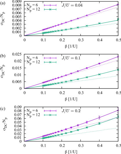
In general, it is expected that a finite-size system with a bounded spectrum exhibits resistivity linear in temperature in the limit (or linear in inverse temperature ) Mukerjee et al. (2006); Patel and Changlani (2022). When working within the canonical ensemble in the strongly interacting limit, the upper bound of the Bose-Hubbard model is close to , where is the number of particles, and all the bosons occupy the same site. Within the grand-canonical ensemble we control the average density by reducing the chemical potential and in this way we effectively limit the highest energy state.
The key question is how far down in the temperature range resistivity linear in temperature persists. In particular, for hard-core bosons it has been shown that higher-order corrections become strong only at low temperatures in the vicinity of the BKT phase transition Lindner and Auerbach (2010). To determine where quadratic corrections to start to play a role, we fit our result to
| (15) |
in the range . We find that this approximation works well even for a wider range . For weak hopping , in agreement with the observation from Fig. 5, we find that , or
| (16) |
A closely related result for the fermionic model has been derived using a high-temperature expansion in Ref. Perepelitsky et al. (2016). For the stronger hopping it holds that , as shown in Fig. 7. The sub-leading term becomes more prominent as the ratio gets stronger.
III.5 The analysis of the Kubo formula
We explain the numerically identified features of the conductivity using the framework introduced in Ref. Patel and Changlani (2022). Starting from the Kubo formula, Eq. (6), we consider small enough . Following the previous numerical analysis, in the following we use small but finite . We approximate the Dirac delta function from Eq. (6) as , where is the Heaviside function, and the bin width is chosen to accommodate a reasonably large number of energy levels of our finite size system. By rewriting Eq. (6) and taking the limit we obtain
| (17) | |||||
where
| (18) |
Using the high-temperature expansion in Eq. (17), we find approximate results for the coefficients and introduced in Eq. (15)
| (19) | |||||
| (20) |
where . By a numerical inspection, we find that estimates for the coefficients and obtained in this way do match numerical data. Based on the approximation in Eq. (19) we infer that behavior is related to the presence of bands in the many-body spectrum. The bands’ density of states is inversely proportional to , see Fig. 1, and consequently the number of available states within a frequency bin in Eq. (18) is inversely proportional to the tunneling . For stronger a quadratic dependence appears as the band structure is washed out, Fig. 7.
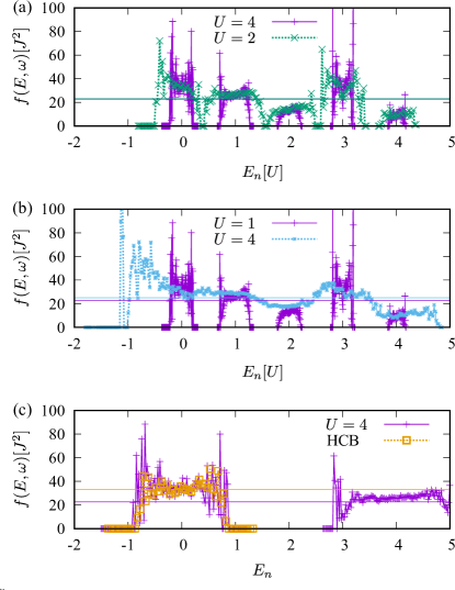
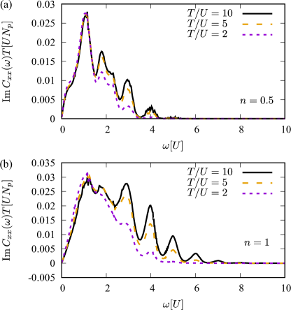
Following Ref. Patel and Changlani (2022) we perform coarse-graining of the coefficients from Eq. (18)
| (21) |
where is the many-body density of states, Eq. (8). An almost flat line, an indicator of the invariance of with energy , ensures resistivity linear in temperature far down in , as shown in Ref. Patel and Changlani (2022). In Fig. 8(a) we present the coarse-grained coefficients for and and . In both cases the many-body spectrum consists of the bands centered around . Within each band is roughly constant and weakly dependent on . As gets weaker, the gaps between bands are closed and the function acquires more features, see Fig. 8(b) for . Because the function deviates from an averaged flat line throughout the spectrum, at first glance the resistivity linear in temperature is found only at high-temperatures. This observation is in agreement with the data presented in Fig. 6 where the regime of linear resistivity is found roughly at (). However, in the next subsection we discuss another regime of linear resistivity found at lower temperatures when the hard-core description becomes relevant.
III.6 Comparison with hard-core bosons
Conductivity of hard-core bosons at half filling was investigated in Refs. Lindner and Auerbach (2010). It was found that a Gaussian function approximates well optical conductivity as a function of frequency. In order to reach the limit of hard-core bosons here we consider bosons at half filling ( bosons per lattice site). We keep fixed hopping rate and change the value of local interaction . In Fig. 9(a) we show that for the low enough ratio , for example for and , our results for the optical conductivity at half filling approach the result for hard-core bosons for as expected. The contribution of higher Hubbard bands is absent in the hard-core model.
The same applies to the DC conductivity as shown in Fig. 9(b). It was shown in Ref. Lindner and Auerbach (2010) that the resistivity of hard-core bosons is linear in temperature down to very low temperatures close to the BKT transition. Our considerations from the previous subsection are in line with this conclusion, as we find the hard-core bosons to exhibit nearly constant function , see Fig. 8(c), that closely corresponds to the function of the lowest band of the full model. As expected, when the temperature is low enough with respect to , only the lowest band of the full model is occupied and bosons can be described as hard-core particles. Consequently, the DC conductivity starts off as a linear function of the inverse temperature , exhibits a transitional behavior for a range of intermediate values, and changes into a linear function corresponding to hard-core boson behavior at large (low ).
Now we investigate in more detail how the DC conductivity of hard-core bosons is reached by varying parameter of the full model and temperature . We present data for the DC conductivity as a function of temperature and interaction in Fig. 10. As we plot the DC conductivity multiplied by temperature , for hard-core bosons we find an almost perfect constant within the considered temperature range, see Fig. 10(a). This constant is reached for at and for at . What we find surprising is the dependence of the conductivity: we find to exhibit a minimum at some finite before reaching the hard-core boson result, see Fig. 10(b).
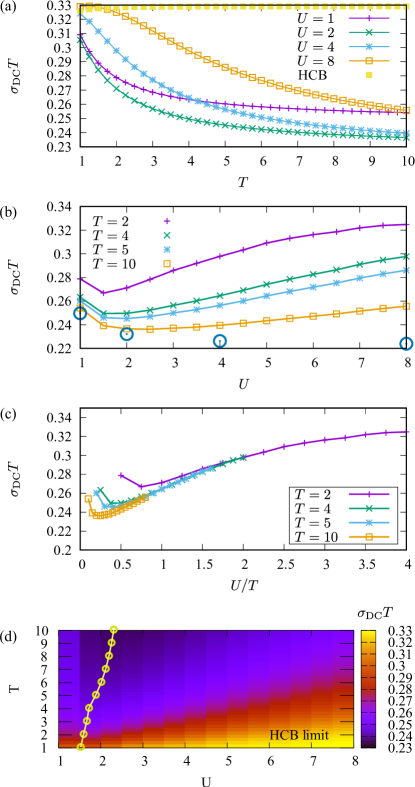
This behavior can be traced back to the result from Fig. 8(c) where we see that the averaged value of of hard-core bosons overestimates the result of the full model. We rewrite Eq. (17) as
| (22) |
and consider the strongly interacting limit where the function can be approximated by a sum of rectangular functions centered around , as presented in Fig. 8(a). From Fig. 8(a) we observe that from the several lowest Hubbard bands, it is the lowest band that has the highest value of . From Eq. (22) we infer that at fixed temperature, as we increase the interaction strength , both the nominator and the denominator of the last expression are reduced. Yet, the partition function decays faster, because each term in the numerator is multiplied with a factor (and getting smaller with increasing ), while in the denominator it is multiplied by one. Therefore, the conductivity increases with increasing U, and we reach the limit of hard-core-boson conductivity from below. This is a striking and highly counterintuitive observation. We have checked that this feature persists even when calculations are done in the grand canonical ensemble, and when the size of the lattice is changed, but it still might be an artifact of the finite size of the system.
III.7 Finite-size effects
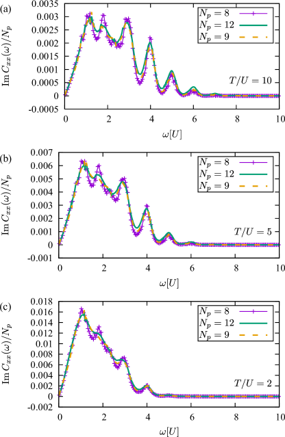
While lattice sizes that we consider are too small to quantitatively predict results in the thermodynamic limit, we expect that the main features of the optical conductivity that we observe remain valid. For example, at high temperature we do expect DC conductivity to take the from , yet the exact value of the tunneling and temperature where this behavior changes into a more-complex dependence is possibly system-size dependent. In Fig. 11 we compare the current-current correlation functions for three different lattice sizes at several values of temperatures. Overall, the results show good agreement and the main discrepancies are found close to .
III.8 The grand-canonical ensemble
Here we consider the grand-canonical ensemble and introduce chemical potential
| (23) |
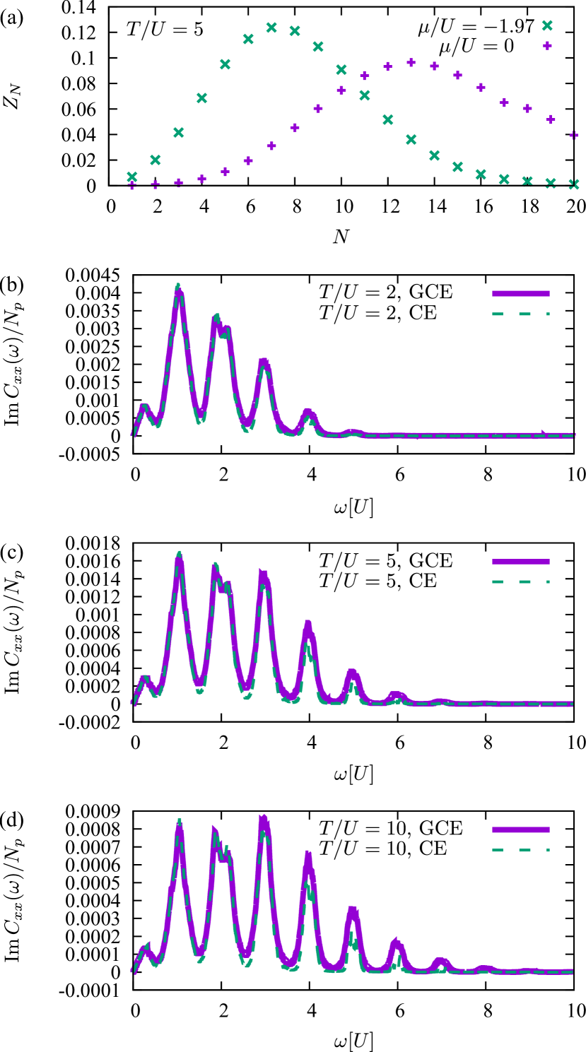
where is number of particles. The value of the chemical potential is set as usual, by requiring certain filling. In Fig. 12 we make a comparison of results obtained in this way with the results presented in the main text within the fixed particle-number sector. We consider small lattice and up to 20 particles. We find that there are some quantitative differences, while the main qualitative features of the correlation function remain unchanged. The contribution of conductivity peaks found at is stronger at high temperatures when we take into account particle-number fluctuations within the grand-canonical ensemble.
III.9 Comparison with bubble-diagram approximation
Here we use the bubble-diagram approximation, that has been extensively used for the calculation of the conductivity within the Fermi-Hubbard model Limelette et al. (2003); Terletska et al. (2011); Vučičević et al. (2013); Deng et al. (2013); Vučičević et al. (2015, 2019); Vranić et al. (2020); Vučičević and Žitko (2021a, b); Vučičević et al. (2023). We find that for small lattices the bubble approximation works well only at high frequencies. Similar relation between the full result and the bubble approximation has been observed in the fermionic Hubbard modelVučičević et al. (2019) and more recently even in the context of Holstein modelJanković et al. (2024). By contrast, however, here vertex corrections appear to reduce conductivity, rather than increase it.
Within the grand-canonical ensemble we first calculate the single-particle Green’s function
| (24) |
where , and are vectors labeling lattice sites. The eigenenergies and and eigenstates and are obtained in two different particle sectors with and particles. From here we obtain the spectral function:
| (25) |
By using the Wick theorem we obtain the bubble-diagram approximation for conductivity:
| (26) |
where is the Bose-Einstein distribution and is the non-interacting dispersion relation on a two dimensional lattice.
We perform numerical test of the accuracy of this approximation by comparing results obtained from Eq. (26) with the full result from Eq. (5). We find that for the small system sizes the approximation works well at higher frequencies , but it fails to reproduce numerical data in the limit as shown in Fig. 13. For we find that the spectral function features separate peaks close to , . From Eq. (26) it follows that the peaks in optical conductivity emerge when the two peaks in and overlap, as for , as discussed in subsection III.
IV Conclusion and discussion
In this paper we investigated optical conductivity of the Bose-Hubbard model in the high-temperature regime. Based on the numerically exact calculation for small lattice sizes, we identified multiple peaks in optical conductivity stemming from the Hubbard bands at weak tunneling . As the tunneling rate gets stronger, these peaks merge, and the conductivity takes simpler form. We analyzed the regime with resistivity linear in temperature and found that the proportionality constant is inversely proportional to the tunneling rate in the limit . Additionally, in some cases we observe two separate linear regimes of different slopes - one at lower temperature corresponding to hard-core boson behavior, and one at high temperature, corresponding to the leading order in -expansion. Finally, we find a striking and unexpected non-monotonic dependence of on the coupling constant. At half-filling and fixed temperature , above some value of , grows with the increasing and eventually it approaches the hard-core-boson conductivity. Further work is necessary to confirm that this feature of our results survives in the thermodynamic limit.
We expect that these results can be probed in cold-atom experiments, along the lines of Ref. Brown et al. (2019). For a quantitative comparison with experiments, it may turn out that additional Hamiltonian terms describing bosons in optical lattices should be taken into account in addition to the Bose-Hubbard model. Moreover, processes beyond the linear-response regime may play a role Roy et al. (2020). In order to extend these calculations to larger system sizes, beyond-mean-field approximations Snoek and Hofstetter (2013); He and Yi (2022); Pohl et al. (2022); Caleffi et al. (2020); Colussi et al. (2022) could be considered.
Computations were performed on the PARADOX supercomputing facility (Scientific Computing Laboratory, Center for the Study of Complex Systems, Institute of Physics Belgrade). We acknowledge funding provided by the Institute of Physics Belgrade, through the grant by the Ministry of Education, Science, and Technological Development of the Republic of Serbia, as well as by the Science Fund of the Republic of Serbia, under the Key2SM project (PROMIS program, Grant No. 6066160). J. V. acknowledges funding by the European Research Council, grant ERC-2022-StG: 101076100.
References
- Bloch et al. (2008) I. Bloch, J. Dalibard, and W. Zwerger, Rev. Mod. Phys. 80, 885 (2008).
- Chien et al. (2015) C.-C. Chien, S. Peotta, and M. di Ventra, Nat. Phys. 11, 998 (2015).
- Krinner et al. (2017) S. Krinner, T. Esslinger, and J.-P. Brantut, J. Phys. Condens. Matter 29, 343003 (2017).
- Brown et al. (2019) P. T. Brown, D. Mitra, E. Guardado-Sanchez, R. Nourafkan, A. Reymbaut, C.-D. Hébert, S. Bergeron, A.-M. S. Tremblay, J. Kokalj, D. A. Huse, P. Schauß, and W. S. Bakr, Science 363, 379– (2019).
- Grigera et al. (2001) S. A. Grigera, R. S. Perry, A. J. Schofield, M. Chiao, S. R. Julian, G. G. Lonzarich, S. I. Ikeda, Y. Maeno, A. J. Millis, and A. P. Mackenzie, Science 294, 329– (2001).
- Cooper et al. (2009) R. A. Cooper, Y. Wang, B. Vignolle, O. J. Lipscombe, S. M. Hayden, Y. Tanabe, T. Adachi, Y. Koike, M. Nohara, H. Takagi, C. Proust, and N. E. Hussey, Science 323, 603 (2009).
- Cao et al. (2018) Y. Cao, V. Fatemi, A. Demir, S. Fang, S. L. Tomarken, J. Y. Luo, J. D. Sanchez-Yamagishi, K. Watanabe, T. Taniguchi, E. Kaxiras, R. C. Ashoori, and P. Jarillo-Herrero, Nature (London) 556, 80 (2018).
- Legros et al. (2018) A. Legros, S. Benhabib, W. Tabis, F. Laliberté, M. Dion, M. Lizaire, B. Vignolle, D. Vignolles, H. Raffy, Z. Z. Li, P. Auban-Senzier, N. Doiron-Leyraud, P. Fournier, D. Colson, L. Taillefer, and C. Proust, Nat. Phys. 15, 142 (2018).
- Licciardello et al. (2019) S. Licciardello, J. Buhot, J. Lu, J. Ayres, S. Kasahara, Y. Matsuda, T. Shibauchi, and N. E. Hussey, Nature (London) 567, 213– (2019).
- Cha et al. (2020) P. Cha, N. Wentzell, O. Parcollet, A. Georges, and E.-A. Kim, Proc. Natl. Acad. Sci. U.S.A. 117, 18341 (2020).
- Deng et al. (2013) X. Deng, J. Mravlje, R. Žitko, M. Ferrero, G. Kotliar, and A. Georges, Phys. Rev. Lett. 110, 086401 (2013).
- Vučičević et al. (2015) J. Vučičević, D. Tanasković, M. J. Rozenberg, and V. Dobrosavljević, Phys. Rev. Lett. 114, 246402 (2015).
- Perepelitsky et al. (2016) E. Perepelitsky, A. Galatas, J. Mravlje, R. Žitko, E. Khatami, B. S. Shastry, and A. Georges, Phys. Rev. B 94, 235115 (2016).
- Vučičević et al. (2019) J. Vučičević, J. Kokalj, R. Žitko, N. Wentzell, D. Tanasković, and J. Mravlje, Phys. Rev. Lett. 123, 036601 (2019).
- Vranić et al. (2020) A. Vranić, J. Vučičević, J. Kokalj, J. Skolimowski, R. Žitko, J. Mravlje, and D. Tanasković, Phys. Rev. B 102, 115142 (2020).
- Kiely and Mueller (2021) T. G. Kiely and E. J. Mueller, Phys. Rev. B 104, 165143 (2021).
- Vučičević et al. (2023) J. Vučičević, S. Predin, and M. Ferrero, Phys. Rev. B 107, 155140 (2023).
- Mukerjee et al. (2006) S. Mukerjee, V. Oganesyan, and D. Huse, Phys. Rev. B 73, 035113 (2006).
- Herman et al. (2019) F. Herman, J. Buhmann, M. H. Fischer, and M. Sigrist, Phys. Rev. B 99, 184107 (2019).
- Patel and Changlani (2022) A. A. Patel and H. J. Changlani, Phys. Rev. B 105, L201108 (2022).
- Vidmar et al. (2013) L. Vidmar, S. Langer, I. P. McCulloch, U. Schneider, U. Schollwöck, and F. Heidrich-Meisner, Phys. Rev. B 88, 235117 (2013).
- Ronzheimer et al. (2013) J. P. Ronzheimer, M. Schreiber, S. Braun, S. S. Hodgman, S. Langer, I. P. McCulloch, F. Heidrich-Meisner, I. Bloch, and U. Schneider, Phys. Rev. Lett. 110, 205301 (2013).
- Snoek and Hofstetter (2007) M. Snoek and W. Hofstetter, Phys. Rev. A 76, 051603 (2007).
- Dhar et al. (2019) A. Dhar, C. Baals, B. Santra, A. Müllers, R. Labouvie, T. Mertz, I. Vasić, A. Cichy, H. Ott, and W. Hofstetter, Phys. Status Solidi B 256, 1800752 (2019).
- Fisher et al. (1989) M. P. A. Fisher, P. B. Weichman, G. Grinstein, and D. S. Fisher, Phys. Rev. B 40, 546 (1989).
- Cha et al. (1991) M.-C. Cha, M. P. A. Fisher, S. M. Girvin, M. Wallin, and A. P. Young, Phys. Rev. B 44, 6883 (1991).
- Kampf and Zimanyi (1993) A. P. Kampf and G. T. Zimanyi, Phys. Rev. B 47, 279 (1993).
- Lindner and Auerbach (2010) N. H. Lindner and A. Auerbach, Phys. Rev. B 81, 054512 (2010).
- Bhattacharyya et al. (2023) S. Bhattacharyya, A. De, S. Gazit, and A. Auerbach, arXiv e-prints , arXiv:2309.14479 (2023), arXiv:2309.14479 [cond-mat.str-el] .
- Sajna et al. (2014) A. S. Sajna, T. P. Polak, and R. Micnas, Phys. Rev. A 89, 023631 (2014).
- Rizzatti and Mueller (2023) E. O. Rizzatti and E. J. Mueller, arXiv e-prints , arXiv:2309.10782 (2023), arXiv:2309.10782 [cond-mat.quant-gas] .
- Chen et al. (2014) K. Chen, L. Liu, Y. Deng, L. Pollet, and N. Prokof’ev, Phys. Rev. Lett. 112, 030402 (2014).
- Lucas et al. (2017) A. Lucas, S. Gazit, D. Podolsky, and W. Witczak-Krempa, Phys. Rev. Lett. 118, 056601 (2017).
- Zeng et al. (2021) T. Zeng, A. Hegg, L. Zou, S. Jiang, and W. Ku, arXiv e-prints , arXiv:2112.05747 (2021), arXiv:2112.05747 [cond-mat.str-el] .
- Hegg et al. (2021) A. Hegg, J. Hou, and W. Ku, Proc. Natl. Acad. Sci. U.S.A. 118, e2100545118 (2021).
- Yue et al. (2023) X. Yue, A. Hegg, X. Li, and W. Ku, New J. Phys. 25, 053007 (2023).
- Yang et al. (2022) C. Yang, H. Liu, Y. Liu, J. Wang, D. Qiu, S. Wang, Y. Wang, Q. He, X. Li, P. Li, Y. Tang, J. Wang, X. C. Xie, J. M. Valles, J. Xiong, and Y. Li, Nature (London) 601, 205 (2022).
- Prelovšek and Bonča (2013) P. Prelovšek and J. Bonča, Springer Series in Solid–State Sciences 176 (2013).
- Capogrosso-Sansone et al. (2008) B. Capogrosso-Sansone, S. G. Söyler, N. Prokof’ev, and B. Svistunov, Phys. Rev. A 77, 015602 (2008).
- Prokof’ev et al. (2001) N. Prokof’ev, O. Ruebenacker, and B. Svistunov, Phys. Rev. Lett. 87, 270402 (2001).
- Mahan (2000) G. D. Mahan, Many Particle Physics, Third Edition (Plenum, New York, 2000).
- Scalapino et al. (1992) D. J. Scalapino, S. R. White, and S. C. Zhang, Phys. Rev. Lett. 68, 2830 (1992).
- Poilblanc (1991) D. Poilblanc, Phys. Rev. B 44, 9562 (1991).
- Gros (1992) C. Gros, Z. Phys. B: Condens. Matter 86, 359 (1992).
- Kollath et al. (2010) C. Kollath, G. Roux, G. Biroli, and A. M. Läuchli, J. Stat. Mech.: Theory Exp. 2010, 08011 (2010).
- Limelette et al. (2003) P. Limelette, P. Wzietek, S. Florens, A. Georges, T. A. Costi, C. Pasquier, D. Jérome, C. Mézière, and P. Batail, Phys. Rev. Lett. 91, 016401 (2003).
- Terletska et al. (2011) H. Terletska, J. Vučičević, D. Tanasković, and V. Dobrosavljević, Phys. Rev. Lett. 107, 026401 (2011).
- Vučičević et al. (2013) J. Vučičević, H. Terletska, D. Tanasković, and V. Dobrosavljević, Phys. Rev. B 88, 075143 (2013).
- Vučičević and Žitko (2021a) J. Vučičević and R. Žitko, Phys. Rev. B 104, 205101 (2021a).
- Vučičević and Žitko (2021b) J. Vučičević and R. Žitko, Phys. Rev. Lett. 127, 196601 (2021b).
- Janković et al. (2024) V. Janković, P. Mitrić, D. Tanasković, and N. Vukmirović, (2024), arXiv:2403.18394 .
- Roy et al. (2020) A. Roy, S. Bera, and K. Saha, Phys. Rev. Res. 2, 043133 (2020).
- Snoek and Hofstetter (2013) M. Snoek and W. Hofstetter, in Quantum Gases: Finite Temperature and Non-Equilibrium Dynamics. Edited by Proukakis Nick et al. Published by World Scientific Publishing Co. Pte. Ltd (2013) pp. 355–365.
- He and Yi (2022) L. He and S. Yi, New J. Phys. 24, 023035 (2022).
- Pohl et al. (2022) U. Pohl, S. Ray, and J. Kroha, Ann. Phys. 534, 2100581 (2022).
- Caleffi et al. (2020) F. Caleffi, M. Capone, C. Menotti, I. Carusotto, and A. Recati, Phys. Rev. Res. 2, 033276 (2020).
- Colussi et al. (2022) V. E. Colussi, F. Caleffi, C. Menotti, and A. Recati, SciPost Phys. 12, 111 (2022).