Generalized Multiscale Finite Element Method
for discrete network (graph) models

Abstract

In this paper, we consider a time-dependent discrete network model with highly varying connectivity. The approximation by time is performed using an implicit scheme. We propose the coarse scale approximation construction of network models based on the Generalized Multiscale Finite Element Method. An accurate coarse-scale approximation is generated by solving local spectral problems in sub-networks. Convergence analysis of the proposed method is presented for semi-discrete and discrete network models. We establish the stability of the multiscale discrete network. Numerical results are presented for structured and random heterogeneous networks.

1 Introduction

Multiphysics models on large networks are used in many applications, for example, pore network models in reservoir simulation, epidemiological models of disease spread, ecological models on multispecies interaction, medical applications such as multiscale multidimensional simulations of blood flow, fibrous materials, electric power systems, and many others [1]. In porous media flow simulation, instead of direct numerical simulation of the flow in the exact pore geometry-based Navier-Stokes flow models, one can be approximated by a simplified network model of throats and pores [2]. This technique reduces the computational complexity and allows for simulation using larger computational domains. In simulations of the class of insulation materials that are composed of a large number of fibers, the network models are used to represent the high-conductive fibrous [3, 4] The application of the discrete network model to river network simulations is presented in [5]. The implementation of the model is based on the PETSc library for high-performance computing systems (HPC). The application of the network models to transient hydraulic simulations is considered in [6, 7] and performed for problems such as water distribution in urban distribution systems, oil distribution, and hydraulic generation. In [8], the authors present a graph-based computational framework that facilitates the construction and analysis of large-scale optimization and simulation applications of coupled infrastructure networks. The dynamic optimal electric power flow is simulated using network models in [9, 10]. In [11], traffic flows are considered in complex networks, where the model is based on a graph or network of streets in which vehicles can move. The application of the spatial networks for disease transmission in epidemiological models is considered in [12]. In [13], a cerebral blood flow is modeled as fluid flow driven through a network of resistors by pressure gradients. The authors introduce a vascular graph modeling framework based on these principles to compute blood pressure, flow, and scalar transport in realistic vascular networks. The simulation of blood flow in microvascular networks and the surrounding tissue is considered in [14]. To reduce the computational complexity of this issue, the network structures are modeled by a one-dimensional graph whose location in space is determined by the centerlines of the three-dimensional vessels. Despite eliminating a significant portion of complexity through this approach, efficiently solving the resulting model remains a common challenge. Homogenization and multiscale methods are commonly used techniques for implementing upscaling to manage the extensive computational complexity associated with large network models.

Multiscale problems arise in many areas of science and engineering and typically involve multiple spacial length scales. Traditional numerical methods, such as finite element or finite volume methods, can become prohibitively expensive when the number of degrees of freedom required to capture all relevant scales becomes large. To address this issue, multiscale and homogenization methods have been developed that seek to efficiently capture the essential features of the problem at each length scale. In homogenization methods, the fine-scale problem is replaced by an equivalent coarse-scale problem that captures the essential features of the original problem at a lower computational cost [15, 16, 17, 18]. The effective properties for the coarse grid approximation are computed by analyzing the behavior of unit cells. The most common homogenization method is based on periodicity, which assumes that the fine-scale problem can be represented as a periodic array of repeating unit cells. Compared to the homogenization techniques, a multiscale methods form a broader class of numerical techniques, for example, the Multiscale Finite Element Method [19, 20], the Heterogeneous Multiscale Method [21], the Local Orthogonal Decomposition method [22], the Variational Multiscale Method [23], the Generalized Multiscale Finite Element Method [24, 25], the Multiscale Finite Volume Method [26, 27] and many others. Most multiscale methods are based on constructing the multiscale basis functions in the local domains to capture fine-scale behavior.

There are various applications of multiscale and upscaling methods for network problems that have been studied extensively. Upscaling traffic flows in complex networks is considered in [11]. The problem is considered in two-dimensional regions whose size (macroscale) is much greater than the characteristic size of the network arcs (microscale). The numerical upscaling method is presented in [28], where a finite element approximation with a localized orthogonal decomposition method represents the macroscale model. Moreover, the application to a two-dimensional network model of paper-based materials in the form of fiber networks is considered [4, 29]. In [1], the nodal displacement in a fiber network model is analyzed using a multiscale method based on the LOD. In [30, 31], the heterogeneous multiscale method (HMM) is proposed to couple a network model on the microscale with a continuum scale over the same physical domain. The coarsening procedures for graph Laplacian problems written in a mixed saddle point form were presented in [32, 33]. The numerical methods for computing the effective heat conductivity of fibrous insulation materials are presented in [3]. The fast algorithm is constructed based on the upscaling procedure. It contains the solution of the auxiliary boundary value problems of the steady-state heat equation in a representative elementary volume occupied by fibers and air. The presented approach ignores air and is further simplified by taking advantage of the slender shape of the fibers and assuming that they form a network. A multiscale method for networks representing flows in a porous medium is presented in [30, 31]. In [34], the mortar coupling is presented to couple pore-scale network models to additional pore-scale or continuum-scale models using mortars. Mortars are finite-element spaces in two dimensions connecting distinct subdomains by ensuring pressure and flux continuity at their shared interfaces. In [13], a cerebral blood flow is modeled as fluid flow in a complex network. The authors construct an upscaling algorithm that significantly reduces the computational cost. Furthermore, the upscaled model no longer requires extensive information regarding the topology of the capillary bed. The reduction of the computational complexity of the simulation of blood flow in microvascular networks and the surrounding tissue is considered in [14]. The authors employ homogenization to the microvascular network’s fine-scale structures in the study, leading to a new hybrid approach. This approach models the fine-scale structures as a heterogeneous porous medium, while the larger vessels’ flow is modeled using one-dimensional flow equations.

This paper introduces the novel approach for upscaling the complex network model based on the Generalized Multiscale Finite Element Method [24, 25]. The GMsFEM has a significant advantage in incorporating small-scale features from heterogeneities into coarse-grid basis functions. The multiscale basis functions are constructed by solving local eigenvalue problems. The online solutions can be calculated for any suitable boundary condition or forcing by these greatly reduced-dimension multiscale basis functions. In this work, we present the construction of the reduced-order model for complex, highly heterogeneous networks. The network model represents the fine-scale model. In contrast, the coarse-scale approximation is represented by a much coarser finite element mesh than the fine-scale network. We design multiscale basis functions to account for the networks’ microscale features by solving the local spectral problems in the primary local network cluster. The constructed multiscale approximation can handle highly varying connectivity and random network structure with a huge system size reduction. Convergence analysis of the proposed method is presented for semi-discrete and discrete network models. We establish the stability of the multiscale discrete network for implicit approximation. Numerical implementation of the network model is performed based on the DMNetwork framework. DMNetwork is a part of PETSc library [35] for high-resolution multiphysics simulations on the large-scale complex network [6, 7]. DMNetwork provides data and topology management, parallelization for multiphysics systems over a network, and hierarchical solvers. We present the main components of the multiscale method for constructing the coarse-scale system. To test the presented upscaling approach, we consider regular cubic lattice networks with and without random elimination processes and random networks [36, 37]. We show that the multiscale method can provide an accurate solution with a huge system size reduction with fine-scale solution reconstruction.

The paper is organized as follows. In Section 2, we consider the fine-scale model of the complex network in semi-discrete and discrete forms with stability analysis. In Section 3, we present the construction of the coarse-scale model using the multiscale method and provide a priory estimate. The numerical results are presented in Section 4 for structured and random heterogeneous three-dimensional network models. The conclusion and future works discussion are given in Section 5.

2 Problem formulation

We consider network represented as a undirected graph $G=(P,E)$, where $P=\{v_{1},v_{2},...,v_{N_{v}}\}$ is a set of vertices (nodes $v_{i}\in\mathcal{R}^{d}$, $d=2,3$) and $E$ is a set of two-elements subsets of $P$ (connections or edges $e_{ij}=\{v_{i},v_{j}\}$ that connect vertices $v_{i}$ (head) and $v_{j}$(tail) and $i\neq j$). Here $N_{v}$ is the total number of vertices/nodes, and $N_{e}$ is the total number of edges/connections [38]. We suppose that the graph is connected and weighted. Furthermore, we assume that the network is embedded into the rectangular cuboid

$$\Omega=[0,L_{1}]\times...\times[0,L_{d}].$$

In Figures 1, we illustrate the two and three-dimensional networks embedded into the square and cube. For network generation, we use OpenPNM library [36]. We note that the method can be constructed for a general case without embedding it into a hyper-rectangle. However, it will affect the coarse-grid construction, and a more general way should be considered based on the graph partitioning.

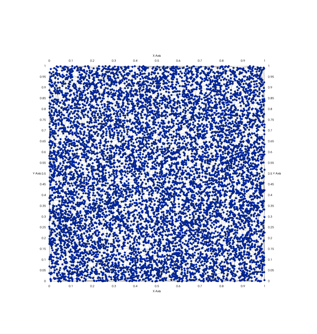
(a) 2D

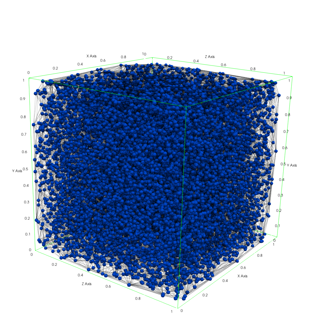
(b) 3D

Figure 1: Illustration of two and three-dimensional networks embedded into the cube

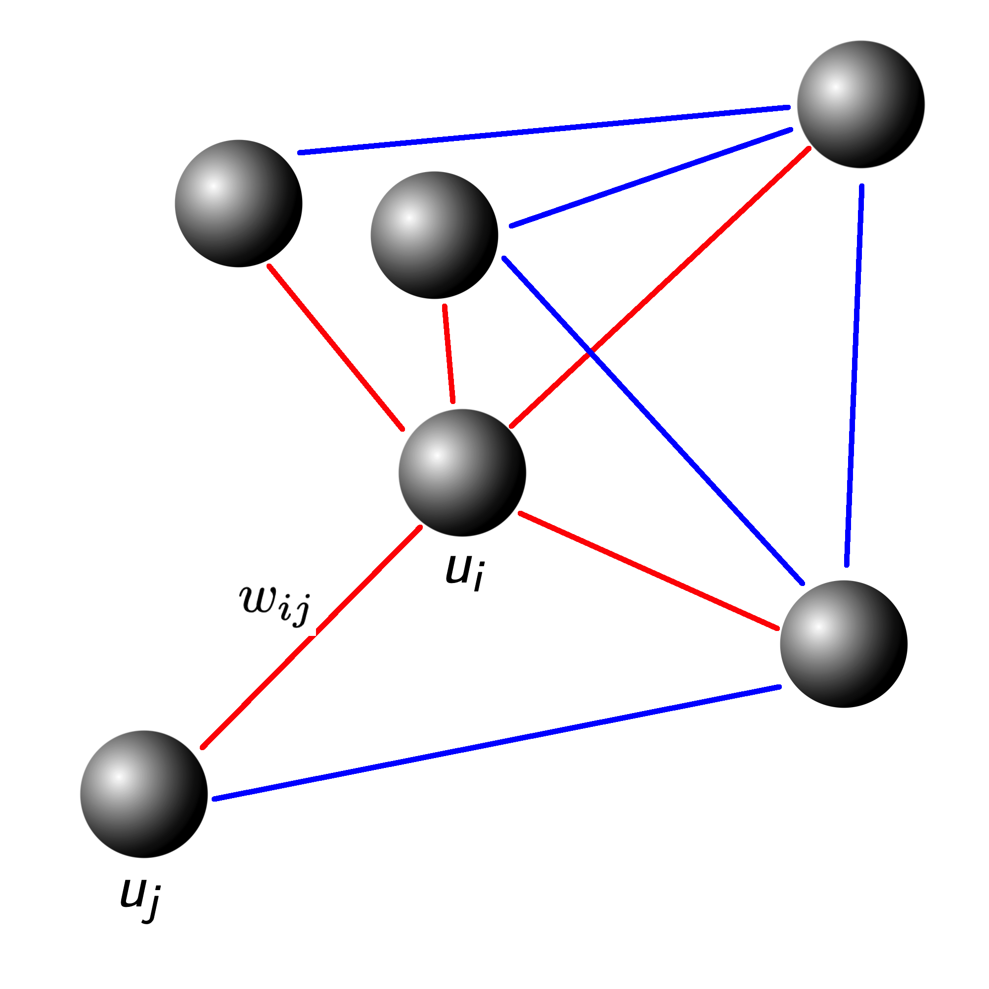
Figure 2: Nodes and connections (edges)

We assign a heterogeneous property $c_{i}$ for each vertex $v_{i}$ that can be associated with the volume in the pore-network model [39]. Then, we associate a weight $w_{ij}$ to each edge proportional to the area of the edge and inversely proportional to the distance between nodes [36] (Figure 2). Additionally, we label nodes associated with the top and bottom boundaries ($\Gamma\subset\partial\Omega$) to set Dirichlet boundary conditions.

Let $D(G)$ be a degree matrix, $W=\{w_{ij}\}_{i,j=1}^{N_{v}}$ be a symmetric weight matrix ($w_{ij}\geq 0$, $w_{ii}=0$ and $w_{ij}>0$ if $e_{ij}$ is an edge) and $L(G)=D(G)-W$ be a graph Laplacian of $G$, where $D(G)=\text{diag}(d_{1},\ldots,d_{N_{v}})$ with $d_{i}=\sum_{j=1}^{N_{v}}w_{ij}$ [38]. Note that we will write $L$ instead of $L(G)$ for simplicity.

For all $u\in\mathcal{R}^{N_{v}}$, we have

$$(Lu)_{i}=\sum_{j\sim i}w_{ij}(u_{i}-u_{j}),$$

where we write $j\sim i$ if nodes $x_{i}$ and $x_{j}$ are connected.

We suppose that $w_{ij}$ are bounded weights ($0<\underline{w}\leq w_{ij}\leq\overline{w}<\infty$) then

$$\begin{split}u^{T}Lu&=u^{T}Du-u^{T}Wu=\sum_{i=1}^{N_{v}}d_{i}u_{i}^{2}-\sum_{i,j=1}^{N_{v}}w_{ij}u_{i}u_{j}\\ &=\frac{1}{2}\left(\sum_{i=1}^{N_{v}}d_{i}u_{i}^{2}-2\sum_{i,j=1}^{N_{v}}w_{ij}u_{i}u_{j}+\sum_{i=1}^{N_{v}}d_{i}u_{i}^{2}\right)=\frac{1}{2}\sum_{i,j=1}^{N_{v}}w_{ij}(u_{i}-u_{j})^{2}\geq 0,\end{split}$$

and operator $L$ is positive semidefinite.

Furthermore, we can write the following representation of the graph Laplacian $L$

$$L=BMB^{T},$$

where matrix $M=\{m_{ij}\}_{i,j=1}^{N_{e}}$ is the diagonal matrix filled with the edge weights and $B=\{b_{ij}\}$ is the vertex-edge incident matrix with size $N_{v}\times N_{e}$ and element $b_{ij}=1$ if $v_{i}$ is a head of edge $e_{j}$, $b_{ij}=-1$ if $v_{i}$ is a tail of edge $e_{j}$ and zero otherwise. Them, we have $(Lu,u)=u^{T}Lu=(B^{T}u)^{T}M(B^{T}u)=\frac{1}{2}\sum_{i,j=1}^{N_{v}}w_{ij}(u_{i}-u_{j})^{2}$.

2.1 Semi-discrete network model

On the weighted undirected graph $G$, we consider the following time-dependent problem

$$c_{i}\frac{\partial u_{i}}{\partial t}+\sum_{j}w_{ij}(u_{i}-u_{j})=f_{i},\quad\forall i\in\mathcal{N},\quad 0<t\leq T,$$ (1)

where $\mathcal{N}=\{1,\ldots,N_{v}\}$ is the set of indexes, $u_{i}$ is defined on on the node $x_{i}$, $f_{i}$ is the given nodal source term and $c_{i}$ is the bounded coefficient, $0<\underline{c}\leq c_{i}\leq\overline{c}<\infty$.

We consider equations (1) with initial conditions

$$u_{i}=u_{i,0},\quad\forall i\in\mathcal{N},\quad t=0,$$

and boundary conditions

$$u_{i}=g_{i},\quad i\in\mathcal{N}_{D},\quad 0<t\leq T,$$

where $\mathcal{N}_{D}$ is the set of node corresponded to the boundary [28].

Let $u=(u_{1},\ldots,u_{N_{v}})^{T}\in\mathcal{R}^{N_{v}}$ be the vector defined on the set of nodes, $f=(f_{1},\ldots,f_{N_{v}})^{T}\in\mathcal{R}^{N_{v}}$ be the given source term vector, and $C$ be the diagonal matrix, $C=\text{diag}(c_{1},\ldots,c_{N_{v}})$. Then we can write problem (2) in the following matrix form

$$C\frac{\partial u}{\partial t}+Lu=f,\quad 0<t\leq T.$$ (2)

with initial conditions $u=u_{0}$ for $t=0$. Note that, in this formulation, the matrices and right-hand side vector are modified to incorporate boundary conditions. For instance, to have a symmetric matrix, we do not include boundary nodes and impose boundary conditions by setting flux on the nodes connected to the boundary.

Let $V\subset\mathcal{R}^{N_{v}}$ be the subspace of real-valued functions defined on the set of nodes satisfying Dirichlet boundary conditions [40]. Then we can write problem formulation in the following equivalent form: find $u\in V$ such that

$$\left(C\frac{\partial u}{\partial t},v\right)+(Lu,v)=(f,v),\quad\forall v\in V,\quad 0<t\leq T,$$ (3)

where $(u,v)=u^{T}v$ and $(Lu,v)=u^{T}Lv$ is scalar products.

Next, we introduce the following two norms $||u||=\sqrt{(u,u)}$ and $||u||_{L}=\sqrt{(Lu,u)}$ and show a stability estimate for a semi-discrete fine-scale scheme (3) [41, 42, 43, 44].

Lemma 1.

The solution of the problem (3) satisfies the following a priory estimate

$$||u(t)||_{L}^{2}\preceq||u_{0}||_{L}^{2}+\int_{0}^{t}||f||^{2}_{C^{-1}}ds.$$ (4)

Proof.

Let $v=\frac{du}{dt}$ in (3) then we have

$$\left(C\frac{du}{dt},\frac{du}{dt}\right)+\left(Lu,\frac{du}{dt}\right)=\left(f,\frac{du}{dt}\right).$$

Using Young’s inequality and $\frac{1}{2}\frac{d}{dt}\left(Lu,u\right)=\left(Lu,\frac{du}{dt}\right)$, we obtain the following estimate

$$\left\|\frac{du}{dt}\right\|^{2}_{C}+\frac{1}{2}\frac{d}{dt}\left(Lu,u\right)=\left(f,\frac{du}{dt}\right)\leq\left\|\frac{du}{dt}\right\|^{2}_{C}+\frac{1}{4}\left\|f\right\|^{2}_{C^{-1}},$$

or

$$\frac{d}{dt}\left\|u\right\|_{L}^{2}\leq\frac{1}{2}\left\|f\right\|^{2}_{C^{-1}}.$$

Finally, after integration by time, we obtain inequality (4) . ∎

2.2 Time-approximation and discrete network model

Let $u^{n}=u(t_{n})$ and $u^{n-1}=u(t_{n-1})$, where $t_{n}=n\tau$, $n=1,2,...$ and $\tau>0$ be the uniform time step size. For approximation by time, we use backward Euler’s to obtain an implicit fully discrete scheme: find $u^{n}\in V$ such that

$$\left(C\frac{u^{n}-u^{n-1}}{\tau},v\right)+(Lu^{n},v)=(f^{n},v),\quad\forall v\in V,\quad n=1,2,...$$ (5)

with initial conditions $u^{0}=u_{0}$. Similarly to the semi-discrete problem (3), we have the following stability estimate [41, 42].

Lemma 2.

The solution of the problem (5) is unconditionally stable and satisfies the following estimate

$$||u^{n}||_{L}^{2}\preceq||u_{0}||_{L}^{2}+\tau\sum_{k=1}^{n}||f^{k}||^{2}_{\left(C+\frac{\tau}{2}L\right)^{-1}}.$$ (6)

Proof.

The equation (5) can be written as follows

$$\left(C\frac{u^{n}-u^{n-1}}{\tau},v\right)+(Lu^{n},v)=\left(\left(C+\frac{\tau}{2}L\right)\frac{u^{n}-u^{n-1}}{\tau},v\right)+\frac{1}{2}(L(u^{n}+u^{n-1}),v)=(f^{n},v).$$

Let $v=\frac{u^{n}-u^{n-1}}{\tau}$ then we have

$$\left(\left(C+\frac{\tau}{2}L\right)\frac{u^{n}-u^{n-1}}{\tau},\frac{u^{n}-u^{n-1}}{\tau}\right)+\frac{1}{2}\left(L(u^{n}+u^{n-1}),\frac{u^{n}-u^{n-1}}{\tau}\right)=\left(f^{n},\frac{u^{n}-u^{n-1}}{\tau}\right).$$

Using the following inequality for the right-hand side

$$\left(f^{n},\frac{u^{n}-u^{n-1}}{\tau}\right)\leq\left\|\frac{u^{n}-u^{n-1}}{\tau}\right\|_{\left(C+\frac{\tau}{2}L\right)}^{2}+\frac{1}{4}\left\|f^{n}\right\|_{\left(C+\frac{\tau}{2}L\right)^{-1}}^{2},$$

we obtain the following estimate for $L=L^{T}$

$$\frac{1}{2\tau}\left(L(u^{n}+u^{n-1}),(u^{n}-u^{n-1})\right)=\frac{1}{2\tau}(Lu^{n},u^{n})+\frac{1}{2\tau}(Lu^{n-1},u^{n-1})\leq\frac{1}{4}\left\|f^{n}\right\|_{\left(C+\frac{\tau}{2}L\right)^{-1}}^{2},$$

or

$$||u^{n}||^{2}_{L}\leq||u^{n-1}||^{2}_{L}+\frac{\tau}{2}\left\|f^{n}\right\|_{\left(C+\frac{\tau}{2}L\right)^{-1}}^{2}.$$

∎

We note that the presented discrete network model with implicit approximation by time leads to solving the large system of equations on each time step. To reduce the size of the system, we use a homogenization approach and construct a coarse-scale approximation by introducing local spectral multiscale basis functions.

3 Multiscale model order reduction

Multiscale methods form a broad class of numerical techniques where most multiscale methods are based on constructing the multiscale basis functions in the local domains to capture fine-scale behavior. In this work, we construct a local spectral multiscale basis function for the network model described above and follow the procedure defined in the Generalized Multiscale Finite Element Method (GMsFEM) [45, 25, 46].

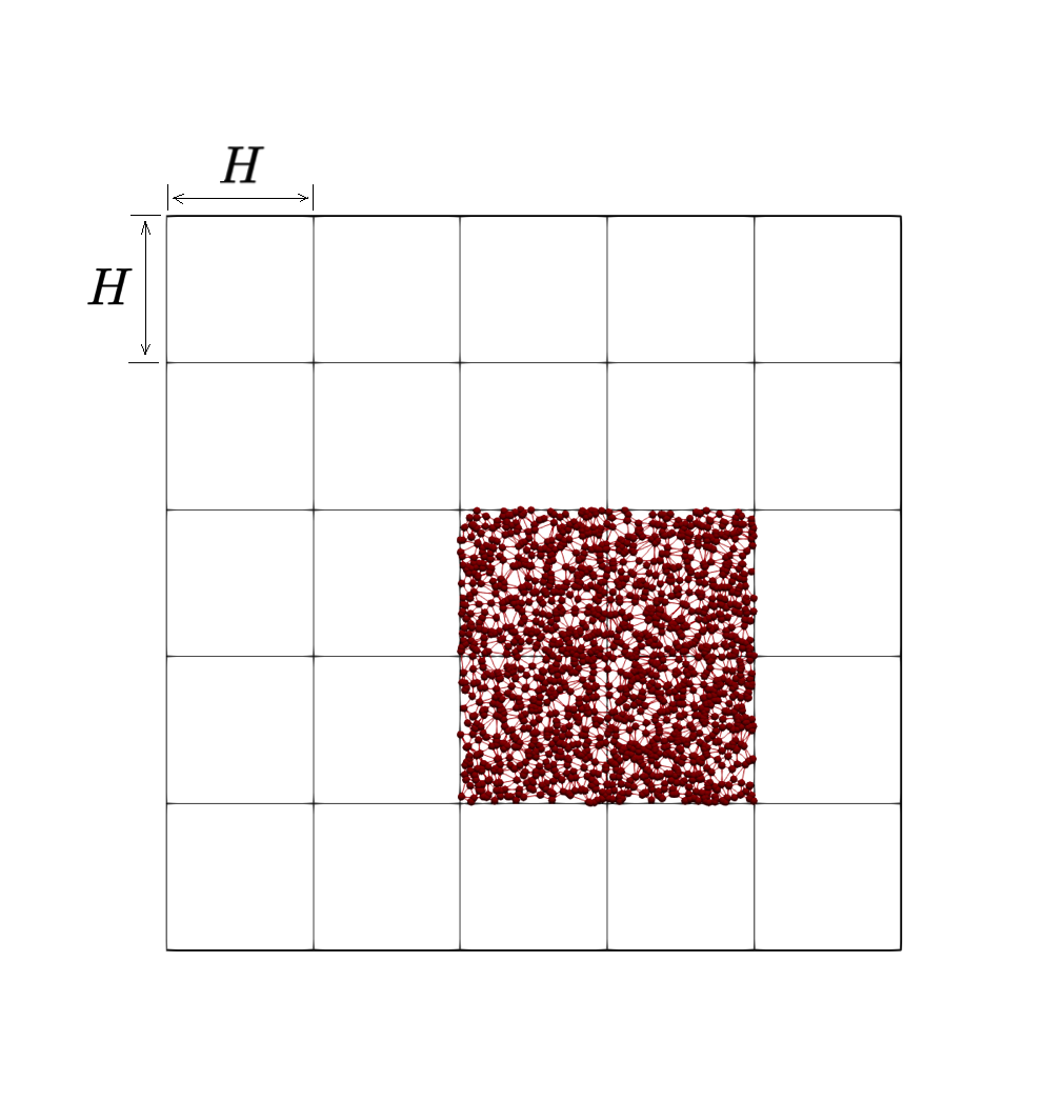
(a) 2D

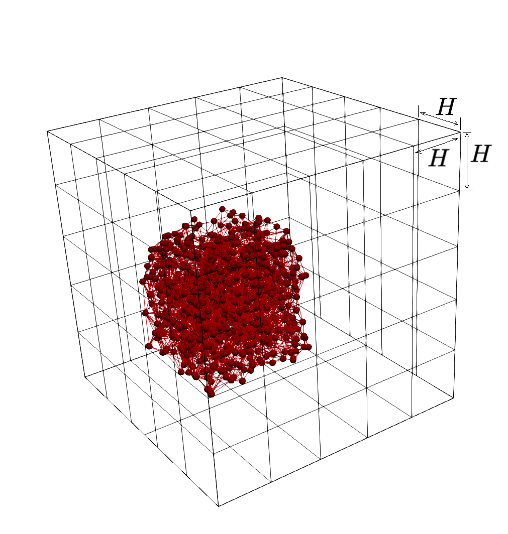
(b) 3D

Figure 3: Illustration of coarse grid $\mathcal{T}_{H}$ and local domain $\omega_{i}$ with sub-network $G^{\omega_{i}}$

Let $\mathcal{T}_{H}$ be a coarse mesh in $\Omega$

$$\mathcal{T}_{H}=\bigcup_{i=1}^{N_{c}}K_{i},$$

where $K_{i}$ is the coarse cell, and $N_{c}$ is the number of coarse cells. We denote $\{y_{i}\}_{i=1}^{N}$ the nodes of the coarse mesh $\mathcal{T}_{H}$, where $N$ is the number of coarse grid nodes [47]. We define $\omega_{i}$ as a neighborhood of the node $y_{i}$

$$\omega_{i}=\bigcup\{K_{j}\in\mathcal{T}_{H}:\ y_{i}\in\bar{K_{j}}\},$$

and $\omega^{K_{j}}$ as a the neighborhood of the element ${K_{j}}$

$$\omega^{K_{j}}=\bigcup\{\omega_{i}:K_{j}\in\omega_{i}\}.$$

In this work we suppose that $\Omega=[0,L_{1}]\times...\times[0,L_{d}]$, where $d=2,3$ is the dimension. Furthermore, we consider a uniform mesh with square and cubic cells for simplicity

$$K_{i}=[y_{i},y_{i}+He_{1}]\times...\times[y_{i},y_{i}+He_{d}],$$

where $H$ is the coarse grid size.

Next, we associate a sub-network $G^{\omega_{i}}$ to each $\omega_{i}$. In Figure 3, we depict a coarse $5\times 5$ mesh for 2D network and $5\times 5\times 5$ coarse grid for 3D network with local domain $\omega_{i}$ and corresponded sub-network $G^{\omega_{i}}$. Note that in implementing the sub-network extraction, we ensure that any node from the global graph $G$ is contained on exactly one coarse element.

The objective of this paper is to develop and analyze a multiscale finite element method for discrete network models defined above. The main idea of the multiscale method is in construction of the coarse-scale approximation of the network by construction of the accurate multiscale basis functions $\{\psi^{ms}_{r,i}\}_{r=1}^{M_{i}}$ in each local domain $G^{\omega_{i}}$ (sub-network), where $M_{i}$ is the number of local basis functions. In the multiscale method, we define offline and online stages:

• Offline stage:

  • Coarse grid ($\mathcal{T}_{H}$) and local domains construction (sub-network, $G^{\omega_{i}}$).

  • Multiscale space construction by the solution of the local eigenvalue in each $G^{\omega_{i}}$

    $$V_{ms}=\text{span}\{\psi^{ms}_{r,i}:1\leq i\leq N,\ 1\leq r\leq M_{i}\}.$$

• Online stage:

  • Solution of the coarse-scale problem (Galerkin approximation): find $u\in V_{ms}$ such that

    $$\left(C\frac{\partial u_{ms}}{\partial t},v_{ms}\right)+(Lu_{ms},v_{ms})=(f,v_{ms}),\quad\forall v_{ms}\in V_{ms}.$$ (7)

We use a same-time approximation as for fine-scale problem with $u_{ms}^{n}=u_{ms}(t_{n})$, where $t_{n}=n\tau$, $n=1,2,...$ and $\tau>0$. By backward Euler’s scheme, we obtain a fully discrete scheme: find $u_{ms}^{n}\in V_{ms}$ such that

$$\left(C\frac{u_{ms}^{n}-u_{ms}^{n-1}}{\tau},v_{ms}\right)+(Lu_{ms}^{n},v_{ms})=(f^{n},v_{ms}),\quad\forall v_{ms}\in V_{ms},\quad n=1,2,...$$ (8)

Next, we discuss details of the multiscale space construction and coarse-scale model generation with some implementation aspects.

3.1 Multiscale basis functions and algorithm

In this work, we use the OpenPNM [36] to construct a network and assign properties. The constructed network is saved in the text files with the corresponding properties. To implement the numerical solution of the fine-scale discrete network model, we use a PETSc library with DMNetwork framework [6, 7]. DMNetwork provides data and topology management, parallelization for multiphysics systems over a large network, and hierarchical solvers.

For the local network $G^{\omega_{i}}$, we have

$$L(\omega_{i})=D(\omega_{i})-W(\omega_{i}),\quad D(\omega_{i})=\text{diag}(d_{1},\ldots,d_{N_{v}^{\omega_{i}}}),\quad d_{i}=\sum_{j=1}^{N_{v}^{\omega_{i}}}w_{ij},$$

where $W(\omega_{i})$ is the local weight matrix and $N_{v}^{\omega_{i}}$ is the number of nodes of local network $G^{\omega_{i}}$ associated with the local domain $\omega_{i}$.

For the sub-network $G^{\omega_{i}}$, the local matrix $L^{\omega_{i}}$ is positive semidefinite for $w_{ij}>0$. Therefore (1) the eigenvalues $0=\lambda^{\omega_{i}}_{1}\leq\lambda^{\omega_{i}}_{2}\leq\ldots\leq\lambda^{\omega_{i}}_{N_{v}^{\omega_{i}}}$ of $L^{\omega_{i}}$ are real and nonnegative, and there is an orthonormal basis of eigenvectors of $L^{\omega_{i}}$; and (2) the smallest eigenvalue $\lambda^{\omega_{i}}_{1}=0$ and corresponded eigenvector is one [38]. Therefore the dimension of the nullspace of $L^{\omega_{i}}$ (dimension of the multiplicity of the eigenvalue 0) is equal to the number of connected components $C_{1},\ldots,C_{C}$ (clusters) of the local network $G^{\omega_{i}}$. Therefore the vectors $f_{l}$ ($f_{l}=(f_{l,1},\ldots,f_{l,N_{v}^{\omega_{i}}})$ such that $f_{l,j}=1$ if $x_{j}\in C_{l}$ and $f_{j}=0$ otherwise, $l=1,\ldots,C$) are form a basis of the nullspace. In the numerical implementation of the eigenvalue problem solution, we use the SLEPc library [48]. We preprocess the local network $G^{\omega_{i}}$ by extracting the primary cluster on which we solve a local eigenvalue problem. We suppose that the size of the primary cluster is much larger than the others. In order to incorporate disconnected clusters into the local multiscale space, we use indicator vectors $f_{l}$. Note that we can solve an eigenvalue problem in each sufficiently big cluster to incorporate local fine-scale behavior and construct an accurate approximation for the general case. For network preprocessing, we use existing tools from the OpenPNM library [36]. Then, we suppose that $G^{\omega_{i}}$ has no isolated vertices, and therefore the local degree matrix $D^{\omega_{i}}$ contains positive entities and is invertible. Then similarly to the GMsFEM for standard finite element-based definition, we use a generalized eigenvalue problem that gives a good approximation space [25, 47].

To construct a multiscale basis functions in each sub-network $G^{\omega_{i}}$, we solve a local generalized eigenvalue problem

$$L^{\omega_{i}}{\phi}_{r}^{\omega_{i}}=\lambda_{r}^{\omega_{i}}D^{\omega_{i}}{\phi}_{r}^{\omega_{i}}$$ (9)

where $L^{\omega_{i}}=L(\omega_{i})$ and $D^{\omega_{i}}=D(\omega_{i})$ are the matrices defined on the sub-network $G^{\omega_{i}}$.

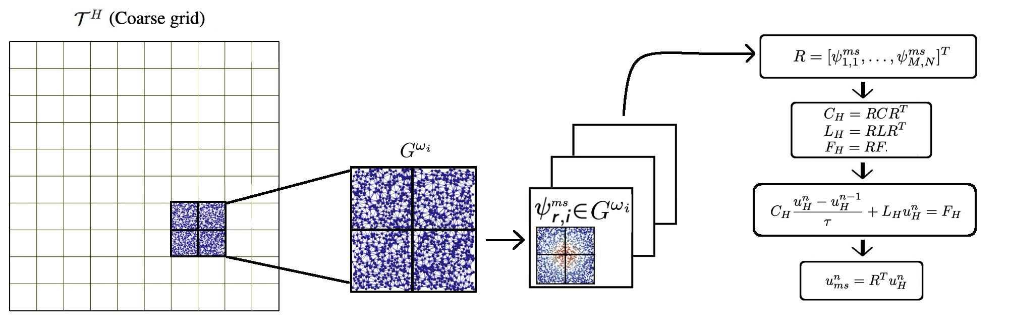
Figure 4: Illustration of steps in the multiscale method

Next, we choose first $M_{i}$ eigenvectors corresponded to the smallest eigenvalues, $\phi_{r}^{\omega_{i}}$, $r=1,\ldots,M_{i}$ in each $G^{\omega_{i}}$ with $i=1,\ldots,N$. In order to form a continuous space, we multiply eigenvalues to the linear partition of unity functions and form a multiscale space

$$V_{ms}=\text{span}\{\psi^{ms}_{r,i}:1\leq i\leq N,\ 1\leq r\leq M_{i}\}.$$

where $\psi^{ms}_{r,i}=\chi_{i}\phi_{r}^{\omega_{i}}$ and $\chi_{i}$ is the projection of the linear partition of unity functions in $\omega_{i}$ to the nodes of corresponded sub-network $G^{\omega_{i}}$.

We implement the presented multiscale algorithm based on the algebraic way by forming the projection matrix

$$R=[\psi^{ms}_{1,1},\ldots,\psi^{ms}_{M_{1},1},\ldots,\psi^{ms}_{1,N},\ldots,\psi^{ms}_{M_{N},N}]^{T}.$$

To define a coarse grid approximation, we use a projection matrix and form a coarse-scale matrix and right-hand side vector

$$C_{H}=RCR^{T},\quad L_{H}=RLR^{T},\quad F_{H}=RF.$$

Finally, we solve a coarse-scale system each time $t_{n}$

$$C_{H}\frac{u_{H}^{n}-u_{H}^{n-1}}{\tau}+L_{H}u_{H}^{n}=F_{H},$$

and reconstruction of the fine-scale solution $u^{n}_{ms}=R^{T}u^{n}_{H}$. The illustration of the main steps of the algorithm is depicted in Figure 4. We note that all offline calculations are independent for each local domain $\omega_{i}$ and can be done entirely parallelly. All coupling is done on the coarse level and generally does not require parallelization. However, for large systems, the size of the coarse-scale approximation can still lead to the large system, and further parallelization of the linear system solution at time $t_{n}$ can be done based on the PETSc implementation of the parallel linear or nonlinear solvers (KSP and SNES classes). Furthermore, the more advanced models can be upscaled similarly with advanced time-stepping techniques available in the TS framework of PETSc. We will consider such advanced coupling in future works.

3.2 Convergence analysis

In this part of the work, we present a priory error estimate of the multiscale method for network models. We note that the analysis presented below is closely related to the analysis in [24, 47, 49, 50, 51]. We start with the definition of global norms used in the presented analysis.

Let $d(u,u)=(Du,u)=u^{T}Du$ and $A=D^{-1}L$ then

$$\begin{split}&d(u,u)=||u||^{2}_{D},\\ &d(Au,u)=(Au)^{T}Du=u^{T}A^{T}Du=u^{T}(D^{-1}L)^{T}Du=u^{T}Lu=a(u,u)=||u||^{2}_{L},\\ &d(Au,Au)=(Au)^{T}D(Au)=u^{T}(D^{-1}L)^{T}D(D^{-1}L)u=u^{T}(L^{T}D^{-1}L)u=||Au||^{2}_{D},\end{split}$$

for $D=D^{T}$ and $L=L^{T}$ [47].

For each $\omega_{i}$ ($i=1,\ldots,N$) we define the local projection

$$P_{M_{i}}^{\omega_{i}}v=\sum_{r=1}^{M_{i}}(v^{T}D^{\omega_{i}}{\phi}_{r}^{\omega_{i}}){\phi}_{r}^{\omega_{i}},$$ (10)

for $v\in V$ and given $M_{i}$ in the local eigenvalue problem (9).

For $P_{M_{i}}^{\omega_{i}}$ the following inequalities holds [47, 50]

$$\begin{split}&||v-P_{M_{i}}^{\omega_{i}}v||^{2}_{D^{\omega_{i}}}\leq\frac{1}{\lambda_{M_{i}+1}^{\omega_{i}}}||v-P_{M_{i}}^{\omega_{i}}v||^{2}_{L^{\omega_{i}}}\leq\frac{1}{\lambda_{M_{i}+1}^{\omega_{i}}}||v||^{2}_{L^{\omega_{i}}},\\ &||v-P_{M_{i}}^{\omega_{i}}v||^{2}_{D^{\omega_{i}}}\leq\frac{1}{(\lambda_{M_{i}+1}^{\omega_{i}})^{2}}||A(v-P_{M_{i}}^{\omega_{i}}v)||^{2}_{D^{\omega_{i}}}\leq\frac{1}{(\lambda_{M_{i}+1}^{\omega_{i}})^{2}}||Av||^{2}_{D^{\omega_{i}}},\\ &||v-P_{M_{i}}^{\omega_{i}}v||^{2}_{L^{\omega_{i}}}\leq\frac{1}{\lambda_{M_{i}+1}^{\omega_{i}}}||A(v-P_{M_{i}}^{\omega_{i}}v)||^{2}_{D^{\omega_{i}}}\leq\frac{1}{\lambda_{M_{i}+1}^{\omega_{i}}}||Av||^{2}_{D^{\omega_{i}}}.\end{split}$$ (11)

Next, we define the coarse projection $\Pi:V\rightarrow V_{ms}$ by

$$\Pi v=\sum_{l=1}^{N}\chi_{l}(P_{M_{l}}^{\omega_{l}}v).$$ (12)

and $v-\Pi v=\sum_{l=1}^{N}\chi_{l}(v-P_{M_{l}}^{\omega_{l}}v)$.

Lemma 3.

Assume that $u\in V$ is the fine scale solution of (3) then the following estimate holds

$$\begin{split}||u-\Pi u||_{D}^{2}\leq\frac{1}{\lambda_{M+1}^{2}}||Au||^{2}_{D}\end{split}$$

where $\lambda_{M+1}=\min_{K}\lambda_{K,M+1}$ and $\lambda_{K,M+1}=\min_{y_{l}\in K}\lambda_{M_{l}+1}^{\omega_{l}}$.

Proof.

Using that $\chi_{l}\leq 1$ we have

$$||u-\Pi u||_{D^{K}}^{2}\leq\sum_{y_{l}\in K}||\chi_{l}(v-P_{M_{l}}^{\omega_{l}}u)||^{2}_{D^{K}}\leq\sum_{y_{l}\in K}||u-P_{M_{l}}^{\omega_{l}}u||_{D^{\omega_{l}}}^{2}.$$

By combing with estimate (11), we obtain the result. ∎

Lemma 4.

Assume that $u\in V$ is the fine scale solution of (3) then the following estimate holds

$$||u-\Pi u||_{L}^{2}\leq\left(\frac{1}{H^{2}\lambda_{M+1}^{2}}+\frac{1}{\lambda_{M+1}}\right)||Au||^{2}_{D}$$

where $\lambda_{M+1}=\min_{K}\lambda_{K,M+1}$ and $\lambda_{K,M+1}=\min_{y_{l}\in K}\lambda_{M_{l}+1}^{\omega_{l}}$.

Proof.

For $z=\{z_{j}\}_{j=1}^{N_{v}}$ with $z_{j}=\chi_{l,j}v_{j}$, we have

$$\begin{split}||z||^{2}_{L^{\omega_{l}}}&=z^{T}L^{\omega_{l}}z=\frac{1}{2}\sum_{i,j=1}^{N^{\omega_{l}}_{v}}w_{ij}(z_{i}-z_{j})^{2}=\frac{1}{2}\sum_{i,j=1}^{N^{\omega_{l}}_{v}}w_{ij}(\chi_{l,i}v_{i}-\chi_{l,j}v_{j})^{2}\\ &=\frac{1}{2}\sum_{i,j=1}^{N^{\omega_{l}}_{v}}w_{ij}(\chi_{l,i}(v_{i}-v_{j})-v_{j}(\chi_{l,j}-\chi_{l,i}))^{2}\leq\frac{1}{2}\sum_{i,j=1}^{N^{\omega_{l}}_{v}}w_{ij}\chi_{l,i}^{2}(v_{i}-v_{j})^{2}+\frac{1}{2}\sum_{i,j=1}^{N^{\omega_{l}}_{v}}w_{ij}v_{j}^{2}(\chi_{l,i}-\chi_{l,j})^{2}.\end{split}$$

Then for $z=\chi_{l}(v-P_{M_{l}}^{\omega_{l}}v)$ using properties of partition of unity function [52], we have

$$||u-\Pi u||_{L^{K}}^{2}\leq\sum_{y_{l}\in K}||\chi_{l}(v-P_{M_{l}}^{\omega_{l}}u)||^{2}_{L^{\omega_{l}}}\leq\sum_{y_{l}\in K}\frac{1}{H^{2}}||u-P_{M_{l}}^{\omega_{l}}u||_{D^{\omega_{l}}}^{2}+\sum_{y_{l}\in K}||u-P_{M_{l}}^{\omega_{l}}u||_{L^{\omega_{l}}}^{2}.$$

By combing with estimate (11), we obtain

$$||u-\Pi u||_{L^{K}}^{2}\leq\left(\frac{1}{H^{2}\lambda_{K,M+1}^{2}}+\frac{1}{\lambda_{K,M+1}}\right)\sum_{y_{l}\in K}||Au||^{2}_{D^{\omega_{l}}}$$

with $\lambda_{K,M+1}=\min_{y_{l}\in K}\lambda_{M_{l}+1}^{\omega_{l}}$.

Then, we have

$$\begin{split}||u-\Pi u||_{L}^{2}=\sum_{K\in\mathcal{T}_{H}}||u-\Pi u||_{L^{K}}^{2}&\leq\sum_{K\in\mathcal{T}_{H}}\left(\frac{1}{H^{2}\lambda_{K,M+1}^{2}}+\frac{1}{\lambda_{K,M+1}}\right)\sum_{y_{l}\in K}||A(u-P_{M_{l}}^{\omega_{l}}u)||^{2}_{D^{\omega_{l}}}\\ &\leq\left(\frac{1}{H^{2}\lambda_{M+1}^{2}}+\frac{1}{\lambda_{M+1}}\right)\sum_{y_{l}\in K}||Au||_{D^{\omega_{l}}}^{2},\end{split}$$

with $\lambda_{M+1}=\min_{K}\lambda_{K,M+1}$. ∎

3.2.1 Multiscale semi-discrete network

In this subsection, we consider semi-discrete network (7) and give a priory estimates for multiscale approximation.

Stability estimate derivation is similar to 4. We let $v_{ms}=\frac{du_{ms}}{dt}=(u_{ms})_{t}$ in (7) then we have

$$\left(C(u_{ms})_{t},(u_{ms})_{t}\right)+\left(Lu_{ms},(u_{ms})_{t}\right)=\left(f,(u_{ms})_{t}\right).$$

Then by Young’s inequality, we obtain the following estimate

$$\left\|(u_{ms})_{t}\right\|^{2}_{C}+\frac{1}{2}\frac{d}{dt}\left(Lu_{ms},u_{ms}\right)\leq\left\|(u_{ms})_{t}\right\|^{2}_{C}+\frac{1}{4}\left\|f\right\|^{2}_{C^{-1}}.$$

Then after integration by time, we obtain the following lemma.

Lemma 5.

The solution of the problem (7) satisfies the following a priory estimate

$$||u_{ms}(t)||_{L}^{2}\leq||u_{ms}(0)||_{L}^{2}+\frac{1}{2}\int_{0}^{t}||f||^{2}_{C^{-1}}ds.$$ (13)

Next, we can obtain the error estimate of the GMsFEM for the semi-discrete network model.

Theorem 1.

Assume that $u\in V$ is the fine scale solution of (3) and $u_{ms}\in V_{ms}$ is the multiscale solution of (7) then the following error estimate holds

$$\begin{split}||(u-u_{ms})(t)||_{C}^{2}+\int_{0}^{t}||u-u_{ms}||_{L}^{2}ds&\preceq||(w-u_{ms})(0)||_{C}^{2}+\frac{1}{\lambda_{M+1}^{2}}||Au||^{2}_{D}\\ &+\int_{0}^{t}\left(\left(\frac{1}{H^{2}\lambda_{M+1}^{2}}+\frac{1}{\lambda_{M+1}}\right)||Au||^{2}_{D}+\frac{1}{\lambda_{M+1}^{2}}||(Au)_{t}||^{2}_{D}\right)ds\end{split}$$

Proof.

Subtracting (3) from (7) , we have

$$\left(C(u-u_{ms})_{t},v\right)+(L(u-u_{ms}),v)=0\quad\forall v\in V_{ms}.$$

We write $u-u_{ms}=(u-w)+(w-u_{ms})$ with $w=\Pi u$ and since $w\in V_{ms}$ we take $v=w-u_{ms}$ and obtain

$$\left(C(w-u_{ms})_{t},w-u_{ms}\right)+(L(w-u_{ms}),w-u_{ms})=\left(C(w-u)_{t},w-u_{ms}\right)+(L(w-u),w-u_{ms}).$$ (14)

For the left part of (14), we have

$$\left(C(w-u_{ms})_{t},w-u_{ms}\right)=\frac{1}{2}\frac{d}{dt}||w-u_{ms}||_{C}^{2},\quad(L(w-u_{ms}),w-u_{ms})=||w-u_{ms}||^{2}_{L}.$$

For the right part of (14) by Young’s inequality, we obtain

$$\left(C(w-u)_{t},w-u_{ms}\right)\leq\frac{1}{4\delta_{1}}||(w-u)_{t}||^{2}_{C}+\delta_{1}||w-u_{ms}||^{2}_{C},$$

and

$$(L(w-u),w-u_{ms})\leq\frac{1}{4\delta_{2}}||w-u||^{2}_{L}+\delta_{2}||w-u_{ms}||^{2}_{L}.$$

Combing estimates for right and left parts of (14) with $\delta_{1}=\delta_{2}=1/2$, we can obtain

$$\frac{d}{dt}||w-u_{ms}||_{C}^{2}+||w-u_{ms}||^{2}_{L}\leq||(w-u)_{t}||^{2}_{C}+||w-u_{ms}||^{2}_{C}+||w-u||^{2}_{L}.$$

By the Gronwall Lemma we obtain

$$||(w-u_{ms})(t)||_{C}^{2}+\int_{0}^{t}||w-u_{ms}||^{2}_{L}ds\leq||(w-u_{ms})(0)||_{C}^{2}+\int_{0}^{t}\left(||(w-u)_{t}||^{2}_{C}+||w-u||^{2}_{L}\right)ds.$$

Then using triangle inequality we have

$$\begin{split}||(u-u_{ms})(t)||_{C}^{2}+\int_{0}^{t}||u-u_{ms}||^{2}_{L}ds&\leq||(w-u_{ms})(0)||_{C}^{2}+||(w-u)(t)||_{C}^{2}\\ &+\int_{0}^{t}\left(||(w-u)_{t}||^{2}_{C}+||w-u||^{2}_{L}\right)ds\end{split}$$

Finally with $||u-v||^{2}_{C}\preceq||u-v||^{2}_{D}$ and using Lemmas 3 and 4, we obtain the result. ∎

Note that, we have $Au=D^{-1}Lu=D^{-1}(f-Cu_{t})$ then

$$||Au||_{D}^{2}=||f-Cu_{t}||^{2}_{D^{-1}}.$$ (15)

Therefore the error estimate in Theorem 1 can be written as follows

$$\begin{split}||(u-u_{ms})(t)||_{C}^{2}+\int_{0}^{t}||u-u_{ms}||_{L}^{2}ds&\preceq||(w-u_{ms})(0)||_{C}^{2}+\frac{1}{\lambda_{M+1}^{2}}||f-Cu_{t}||^{2}_{D^{-1}}\\ &+\int_{0}^{t}\left(\left(\frac{1}{H^{2}\lambda_{M+1}^{2}}+\frac{1}{\lambda_{M+1}}\right)||f-Cu_{t}||^{2}_{D^{-1}}+\frac{1}{\lambda_{M+1}^{2}}||(f-Cu_{t})_{t}||^{2}_{D^{-1}}\right)ds\end{split}$$ (16)

If we map the local eigenvalue problem to size one domain [47], then the eigenvalues scale with $H^{-2}$ and we obtain

$$||(u-u_{ms})(t)||_{C}^{2}+\int_{0}^{t}||u-u_{ms}||_{L}^{2}ds\preceq H^{2}\lambda_{M+1}^{-1}$$ (17)

with accurate choose of $u_{ms}(0)$.

3.2.2 Multiscale discrete network

Finally, we present a priory estimate for a fully discrete problem (8).

Stability estimate derivation is similar to Lemma 18. We let $v_{ms}=(u_{ms}^{n}-u_{ms}^{n-1})/\tau$ then

$$\begin{split}\left(C\frac{u_{ms}^{n}-u_{ms}^{n-1}}{\tau},\frac{u_{ms}^{n}-u_{ms}^{n-1}}{\tau}\right)&+(Lu_{ms}^{n},\frac{u_{ms}^{n}-u_{ms}^{n-1}}{\tau})\\ &=\left(\left(C+\frac{\tau}{2}L\right)\frac{u_{ms}^{n}-u_{ms}^{n-1}}{\tau},\frac{u_{ms}^{n}-u_{ms}^{n-1}}{\tau}\right)+\frac{1}{2}\left(L(u_{ms}^{n}+u_{ms}^{n-1}),\frac{u_{ms}^{n}-u_{ms}^{n-1}}{\tau}\right)\\ &=\left(f^{n},\frac{u_{ms}^{n}-u_{ms}^{n-1}}{\tau}\right)\leq\left\|\frac{u_{ms}^{n}-u_{ms}^{n-1}}{\tau}\right\|_{\left(C+\frac{\tau}{2}L\right)}^{2}+\frac{1}{4}\left\|f^{n}\right\|_{\left(C+\frac{\tau}{2}L\right)^{-1}}^{2},\end{split}$$

Then we have

$$\frac{1}{2\tau}\left(L(u_{ms}^{n}+u_{ms}^{n-1}),(u_{ms}^{n}-u_{ms}^{n-1})\right)=\frac{1}{2\tau}(Lu_{ms}^{n},u_{ms}^{n})+\frac{1}{2\tau}(Lu_{ms}^{n-1},u_{ms}^{n-1})\leq\frac{1}{4}\left\|f^{n}\right\|_{\left(C+\frac{\tau}{2}L\right)^{-1}}^{2},$$

or

$$||u_{ms}^{n}||^{2}_{L}\leq||u_{ms}^{n-1}||^{2}_{L}+\frac{\tau}{2}\left\|f^{n}\right\|_{\left(C+\frac{\tau}{2}L\right)^{-1}}^{2}.$$

Lemma 6.

The solution of the problem (8) is unconditionally stable and satisfies the following estimate

$$||u_{ms}^{n}||_{L}^{2}\preceq||u_{ms}^{0}||_{L}^{2}+\tau\sum_{k=1}^{n}||f^{k}||^{2}_{\left(C+\frac{\tau}{2}L\right)^{-1}}.$$ (18)

Next, we present the error estimate of the multiscale method for the discrete network model.

Theorem 2.

Assume that $u^{n}\in V$ is the fine scale solution of (5) and $u^{n}_{ms}\in V_{ms}$ is the multiscale solution of (8) then the following error estimate holds

$$\begin{split}||u^{n}-u^{n}_{ms}||_{C}^{2}+\tau\sum_{k=1}^{n}||u^{k}-u^{k}_{ms}||_{L}^{2}&\preceq||u^{0}-u_{ms}^{0}||_{C}^{2}\\ +&\sum_{k=1}^{n}\left(\tau\left(\frac{1}{H^{2}\lambda_{M+1}^{2}}+\frac{1}{\lambda_{M+1}}\right)||Au^{k}||^{2}_{D}+\frac{1}{\lambda_{M+1}^{2}}||Au^{k}||^{2}_{D}\right).\end{split}$$

Proof.

Subtracting (5) from (8) , we have

$$\left(C\frac{(u^{n}-u^{n}_{ms})}{\tau},v\right)-\left(C\frac{(u^{n-1}-u^{n-1}_{ms})}{\tau},v\right)+(L(u^{n}-u^{n}_{ms}),v)=0\quad\forall v\in V_{ms}.$$

For $u^{n}-u^{n}_{ms}=(w^{n}-u^{n}_{ms})+(u^{n}-w^{n})$ with $w^{n}=\Pi u^{n}$ and $v=w^{n}-u^{n}_{ms}$, we have

$$\begin{split}&\left(C\frac{(w^{n}-u^{n}_{ms})}{\tau},w^{n}-u^{n}_{ms}\right)+(L(w^{n}-u^{n}_{ms}),w^{n}-u^{n}_{ms})\\ &=\left(C\frac{(w^{n}-u^{n})}{\tau},w^{n}-u^{n}_{ms}\right)+\left(C\frac{(u^{n-1}-u_{ms}^{n-1})}{\tau},w^{n}-u^{n}_{ms}\right)+(L(w^{n}-u^{n}),w^{n}-u^{n}_{ms}).\end{split}$$ (19)

For the left part of (19), we have

$$\left(C(w^{n}-u^{n}_{ms}),w^{n}-u^{n}_{ms}\right)=||w^{n}-u^{n}_{ms}||_{C}^{2},\quad(L(w^{n}-u^{n}_{ms}),w^{n}-u^{n}_{ms})=||w^{n}-u^{n}_{ms}||^{2}_{L}.$$

For the right part of (19) by Young’s inequality, we have

$$\left(C(w^{n}-u^{n}),w^{n}-u^{n}_{ms}\right)\leq\frac{1}{4\delta_{1}}||w^{n}-u^{n}||^{2}_{C}+\delta_{1}||w^{n}-u^{n}_{ms}||^{2}_{C},$$

$$\left(C(u^{n-1}-u_{ms}^{n-1}),w^{n}-u^{n}_{ms}\right)\leq\frac{1}{4\delta_{2}}||u^{n-1}-u_{ms}^{n-1}||^{2}_{C}+\delta_{2}||w^{n}-u^{n}_{ms}||^{2}_{C},$$

and

$$(L(w^{n}-u^{n}),w^{n}-u^{n}_{ms})\leq\frac{1}{4\delta_{3}}||w^{n}-u^{n}||^{2}_{L}+\delta_{3}||w^{n}-u^{n}_{ms}||^{2}_{L}.$$

Then with $\delta_{1}=\delta_{2}=1/4$ and $\delta_{3}=1/2$, we obtain

$$||w^{n}-u^{n}_{ms}||_{C}^{2}+\tau||w^{n}-u^{n}_{ms}||^{2}_{L}\preceq||u^{n-1}-u_{ms}^{n-1}||^{2}_{C}+||w^{n}-u^{n}||^{2}_{C}+\tau||w^{n}-u^{n}||^{2}_{L}.$$

Using triangle inequality we have

$$||u^{n}-u^{n}_{ms}||_{C}^{2}+\tau||u^{n}-u^{n}_{ms}||^{2}_{L}\preceq||u^{n-1}-u_{ms}^{n-1}||^{2}_{C}+||w^{n}-u^{n}||^{2}_{C}+\tau||w^{n}-u^{n}||^{2}_{L}.$$

Therefore

$$||u^{n}-u^{n}_{ms}||_{C}^{2}+\tau\sum_{k=1}^{n}||u^{n}-u^{n}_{ms}||^{2}_{L}\preceq||u^{0}-u_{ms}^{0}||^{2}_{C}+\sum_{k=1}^{n}\left(||w^{n}-u^{n}||^{2}_{C}+\tau||w^{n}-u^{n}||^{2}_{L}\right).$$

Finally using Lemmas 3 and 4, we obtain the result. ∎

4 Numerical results

In this section, we present numerical results for the proposed multiscale method.

To test our approach, we consider three networks:

• Network-1: Structured network with 15625 nodes and 45000 edges. This network is related to the finite volume approximation in the heterogeneous domain on the $25\times 25\times 25$ structured grid.

• Network-2: Structured network with dropping out of 12765 nodes and 24718 edges. This network is related to the previous $25\times 25\times 25$ structured grid with an additional dropout procedure, where we randomly remove approximately 20% of nodes and connections with the additional removal of disconnected pores and broken connections to make a ’healthy’ network.

• Network-3: Unstructured network with 15625 nodes and 119713 edges. This random network is formed by the Delaunay tessellation of arbitrary base points implemented in openpnm.

In OpenPNM, we use a Cubic with and without throats, nodes dropping, and random structures (from left to right in Figure 5). Random elimination is applied for some nodes and throats in the second network. After that, the isolated elements and clusters are removed to prevent numerical problems in simulating flow within the network [37]. Next, to generate a heterogeneous property, we randomly assign node volumes, and throat area, find the length of each throat, and calculate the connectivity coefficient based on the area and length of the throat. Additionally, we set labels for nodes on the top and bottom boundaries.

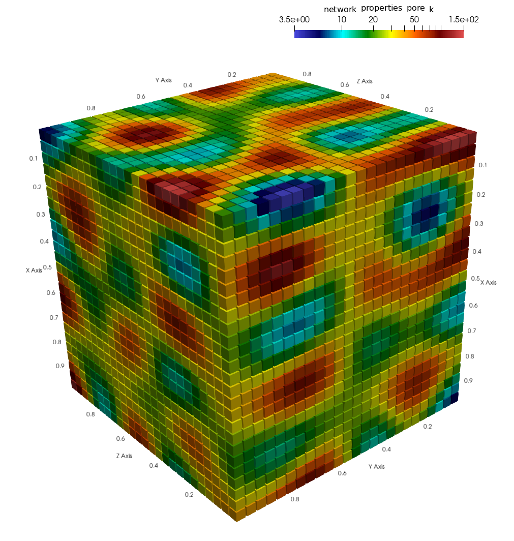
(a) Network-1: Structured (FVM in heterogeneous domain)

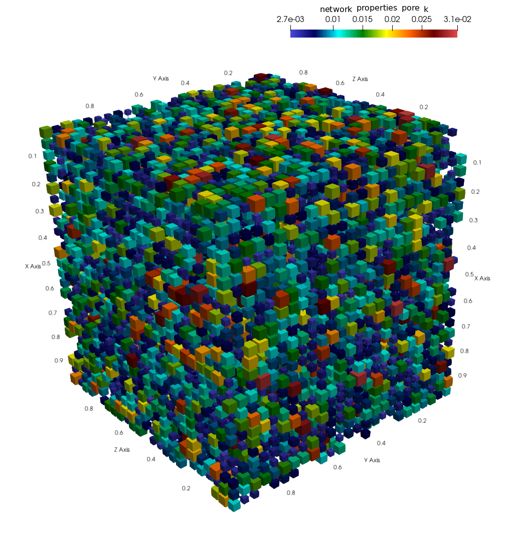
(b) Network-2: Structured with dropout

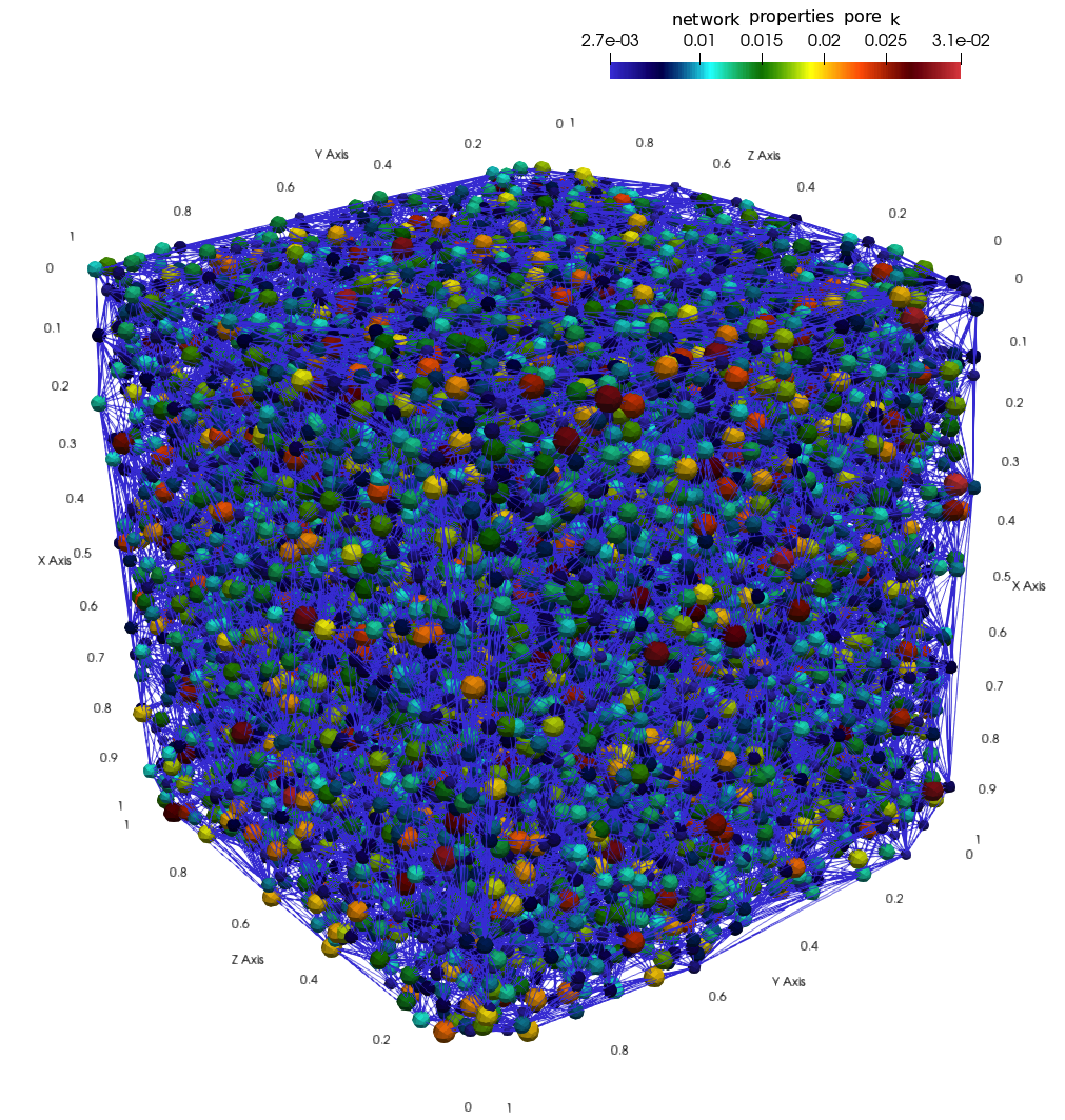
(c) Network-3: Unstructured

Figure 5: Computational domains: Network-1, Network-2, and Network-3

The first network is related to the convenient finite volume approximation of the parabolic equation in the heterogeneous domain. In this network, we assign a heterogeneous diffusion coefficient to each node (cell) and calculate connection weight as a harmonic average of the cell’s coefficients that it connect. For the Network-1, we have $k_{min}=3.49$ and $k_{max}=148.41$ as minimum and maximum for the diffusion coefficient. We have $c_{min}=0.05$ and $c_{max}=0.2$ as minimum and maximum values for the time derivative coefficient. To set heterogeneous properties on the second and third networks, we randomly assign node (pore) size diameters, assign edge (throat) diameters based on the pores it connects, and calculate connection weight based on the throat diameter and distance between pores. This algorithm is convenient in pore-scale simulations using pore network models. For the Network-2, we have $k_{min}=0.0055$ and $k_{max}=0.116$ as minimum and maximum for the connection’s coefficients. For the time derivative coefficient, we have $c_{min}=0.0027$ and $c_{max}=0.03$ as a minimum and maximum for the node’s coefficients. For the Network-3, we have $k_{min}=0.00029$ and $k_{max}=1.45$ as minimum and maximum for the connection’s coefficients. For the time derivative coefficient, we have $c_{min}=0.0027$ and $c_{max}=0.03$ as a minimum and maximum for the node’s coefficients.

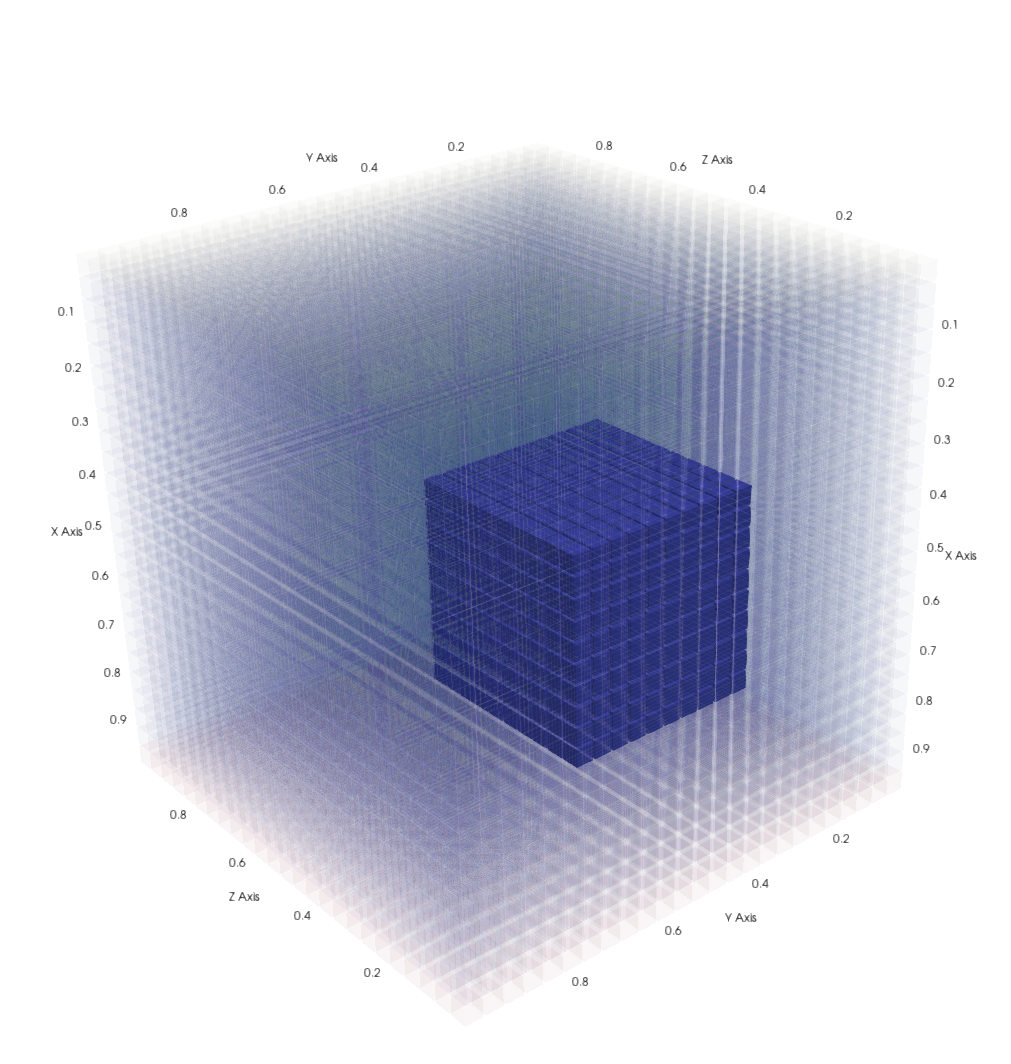
(a) Local domain and Network-1

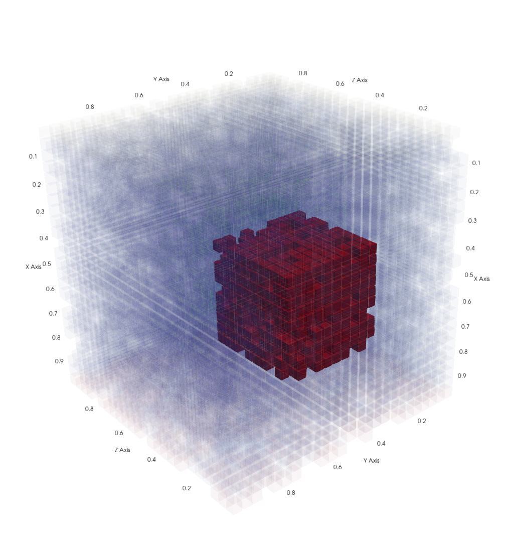
(b) Local domain and Network-2

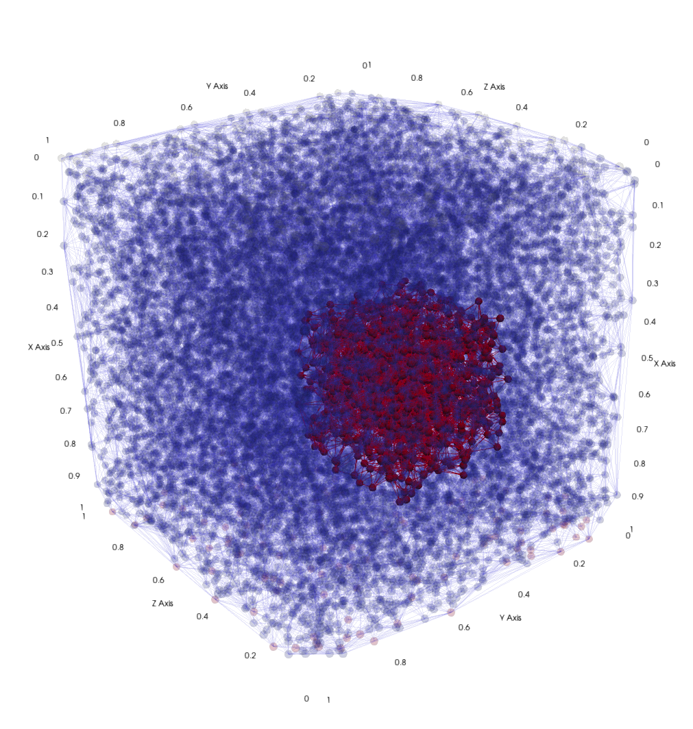
(c) Local domain and Network-3

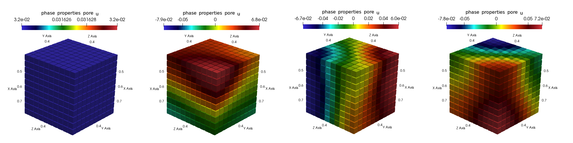
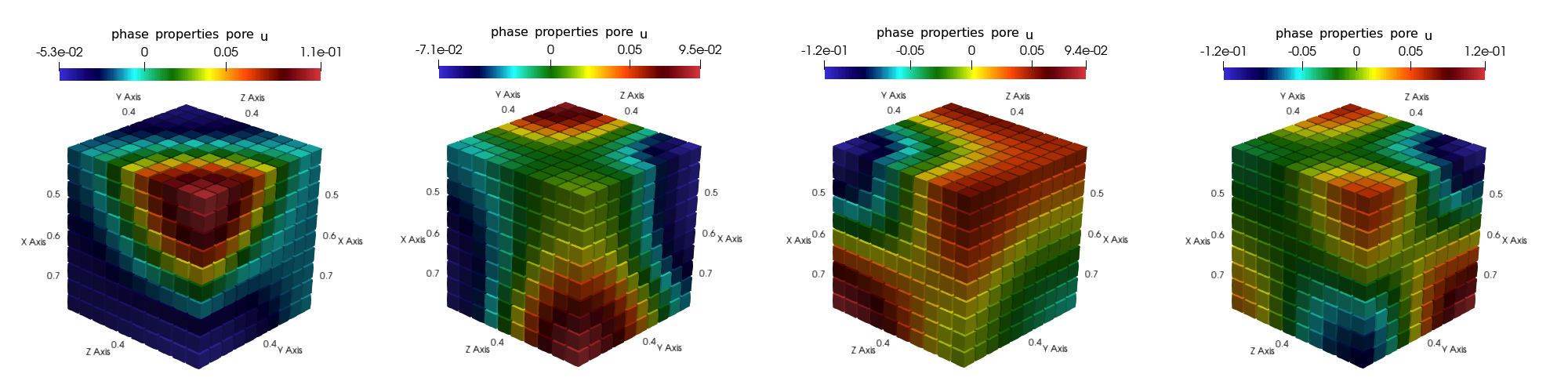
(d) Local eigenvectors for Network-1

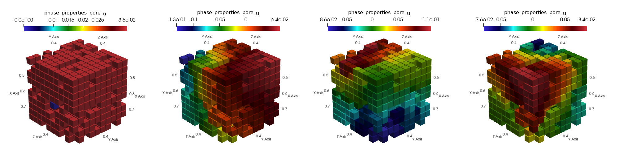
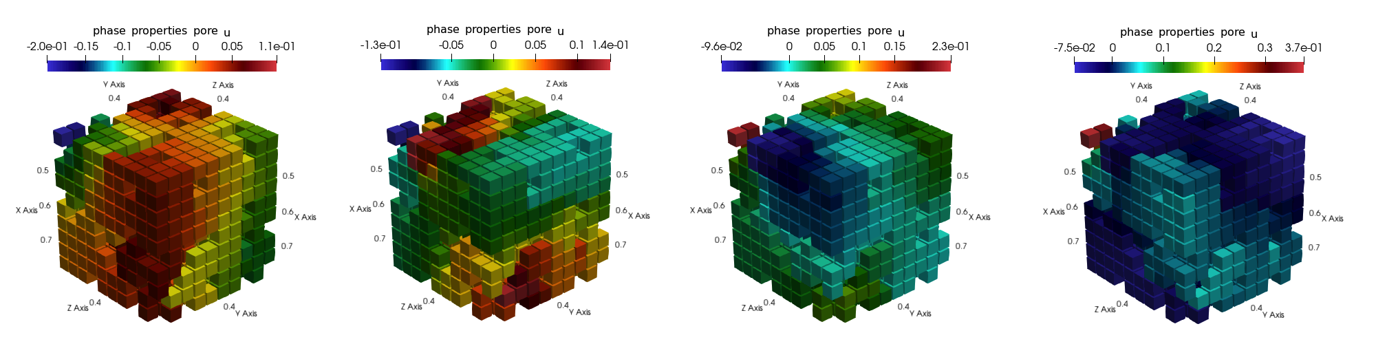
(e) Local eigenvectors for Network-2

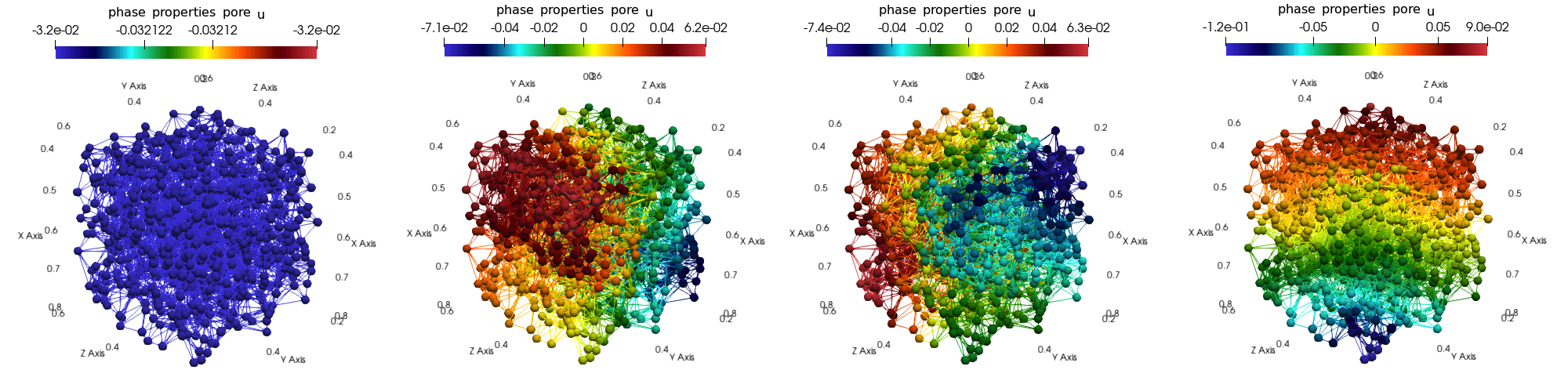
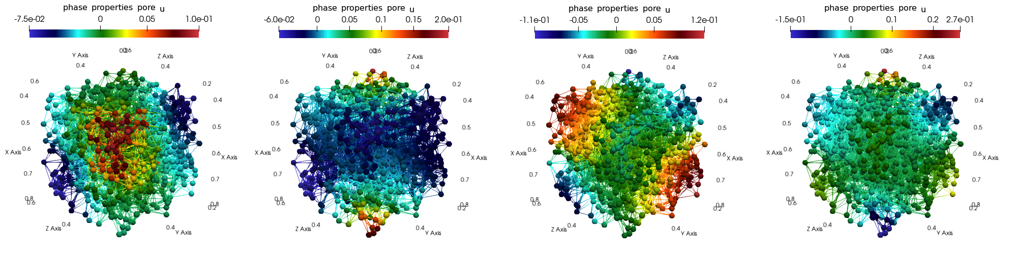
(f) Local eigenvectors for Network-3

Figure 6: Illustration of the local domains with first eight eigenvectors.

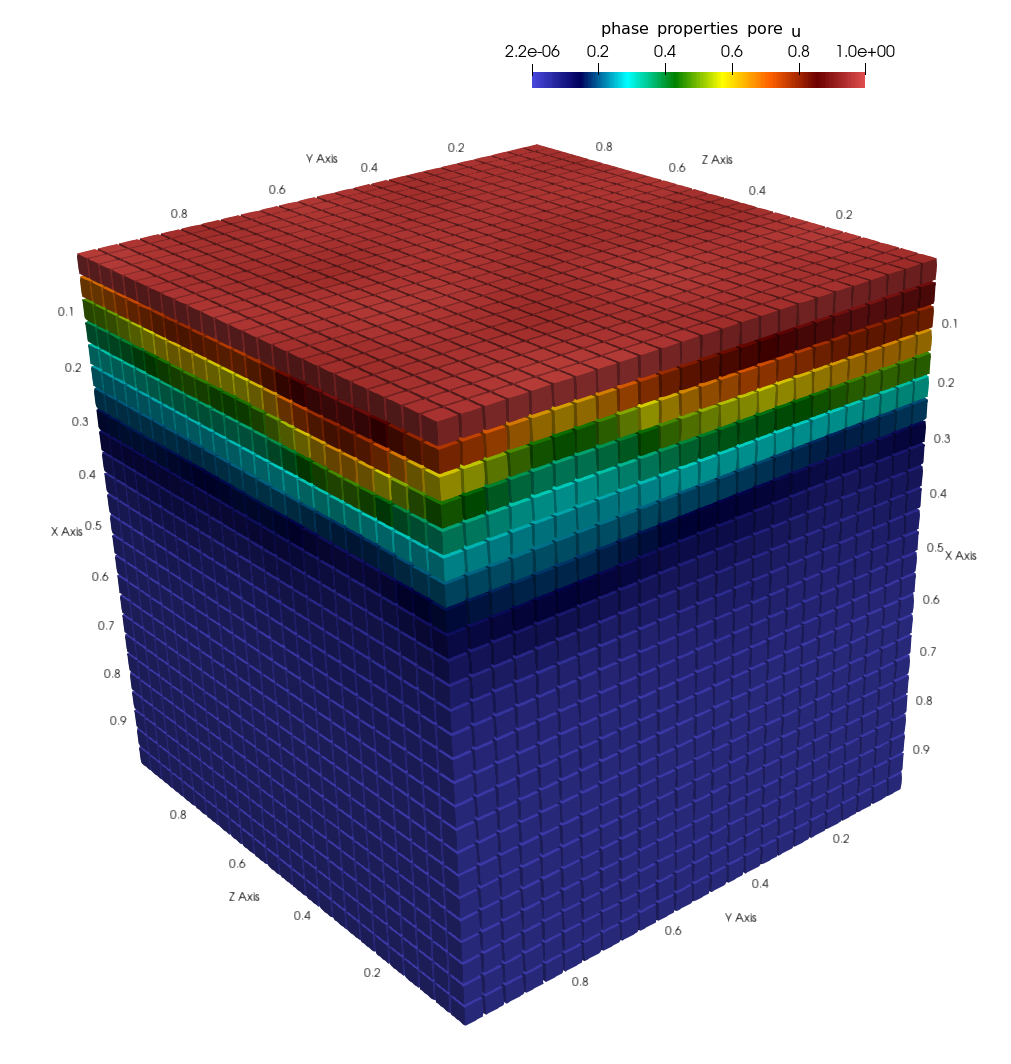
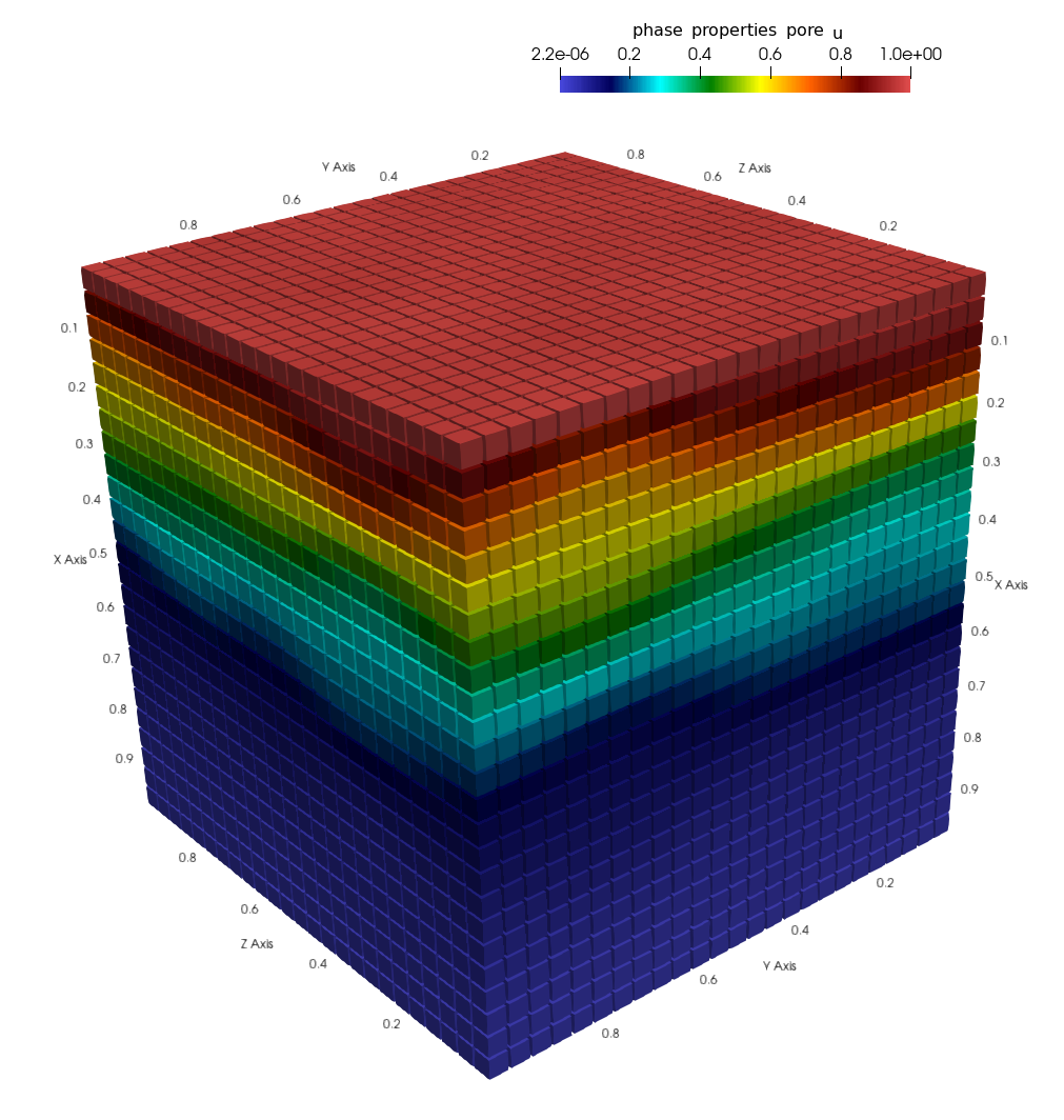
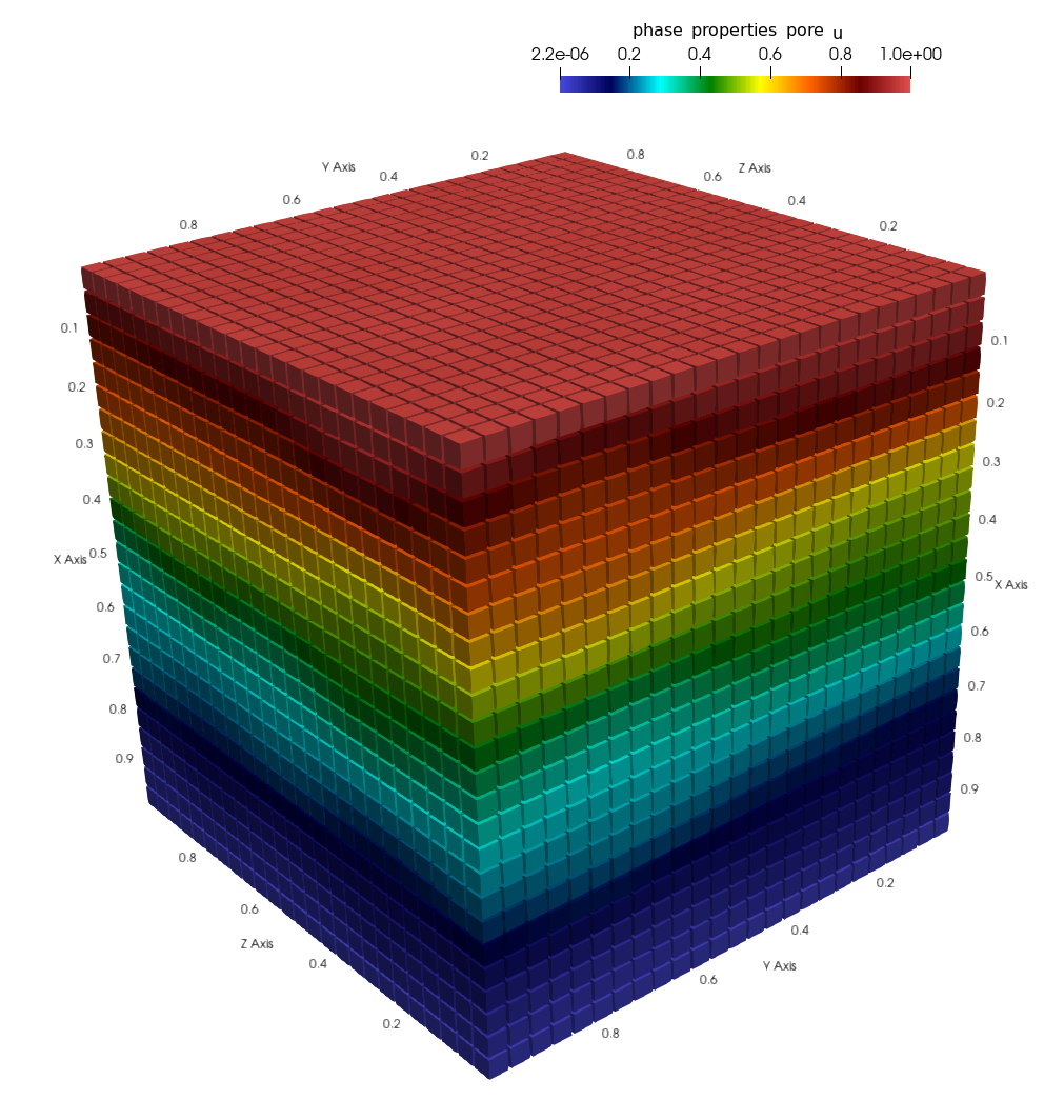
(a) Fine-scale solution: $u^{5}$, $u^{20}$ and $u^{50}$

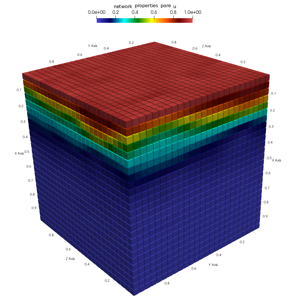
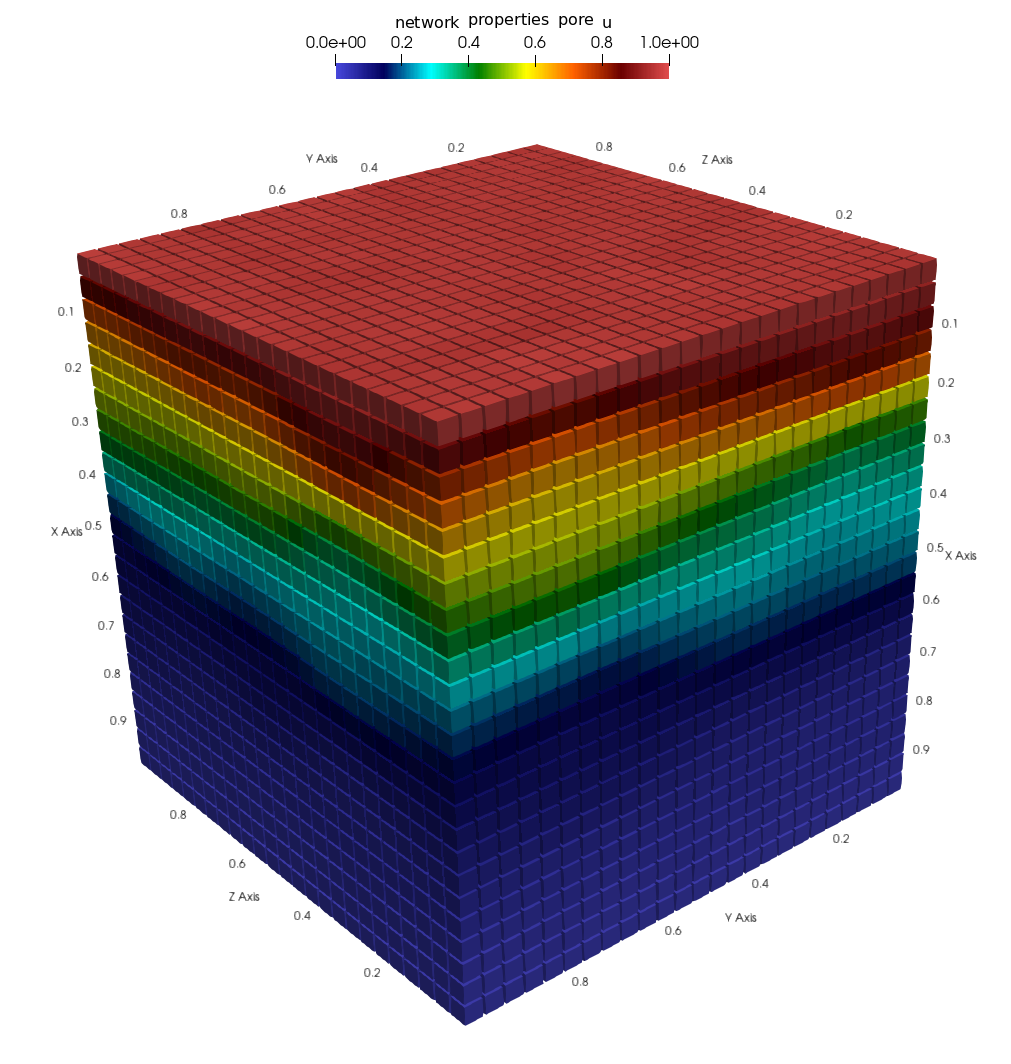
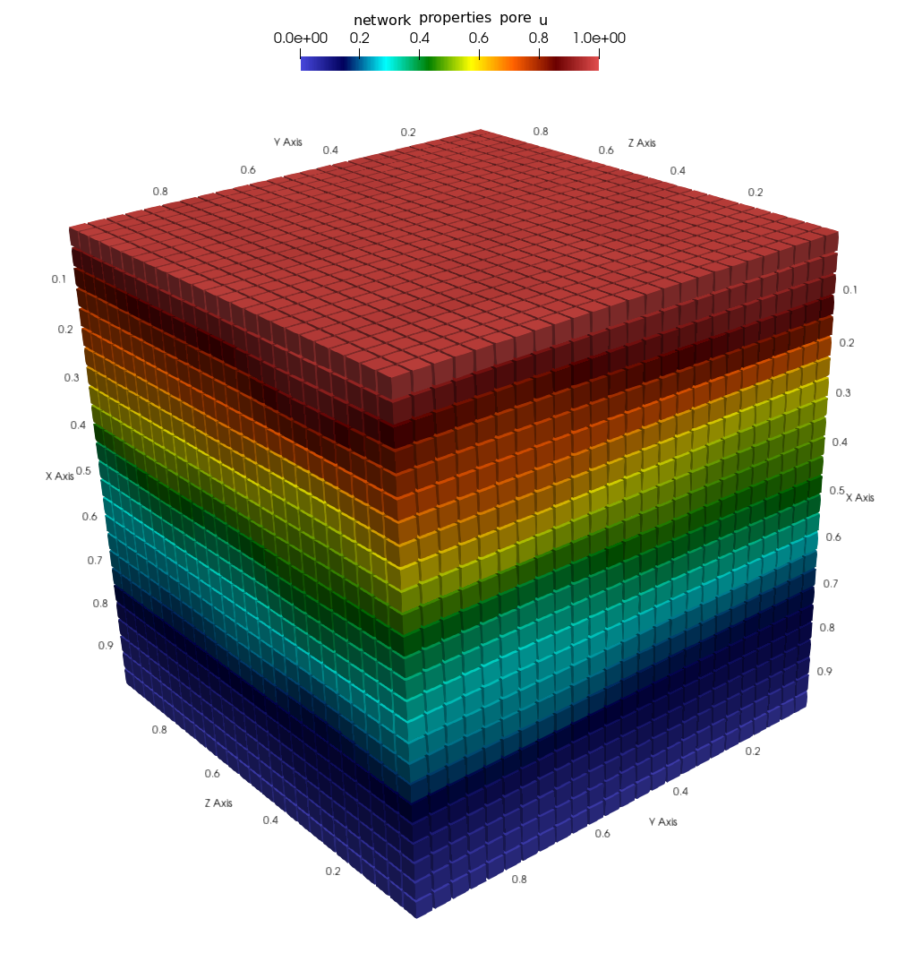
(b) Multiscale solution: $u_{ms}^{5}$, $u_{ms}^{20}$ and $u_{ms}^{50}$

Figure 7: Numerical solution for Network-1.

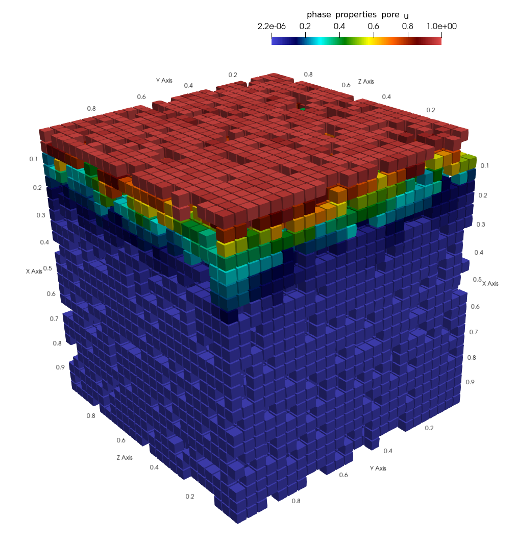
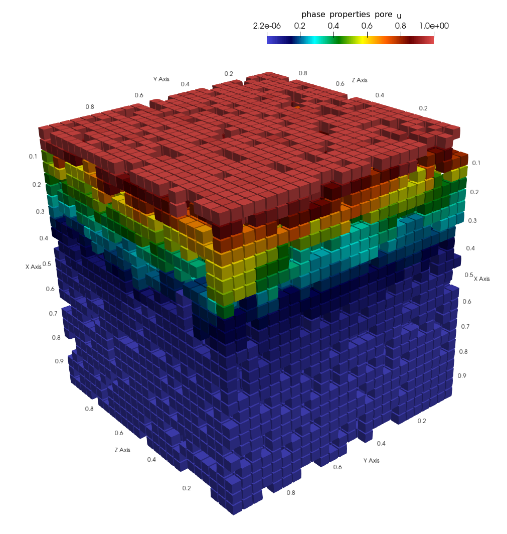
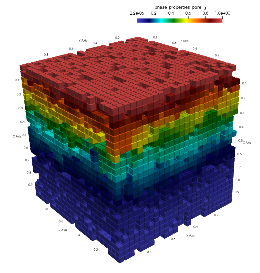
(a) Fine-scale solution: $u^{5}$, $u^{20}$ and $u^{50}$

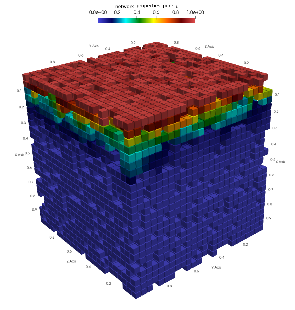
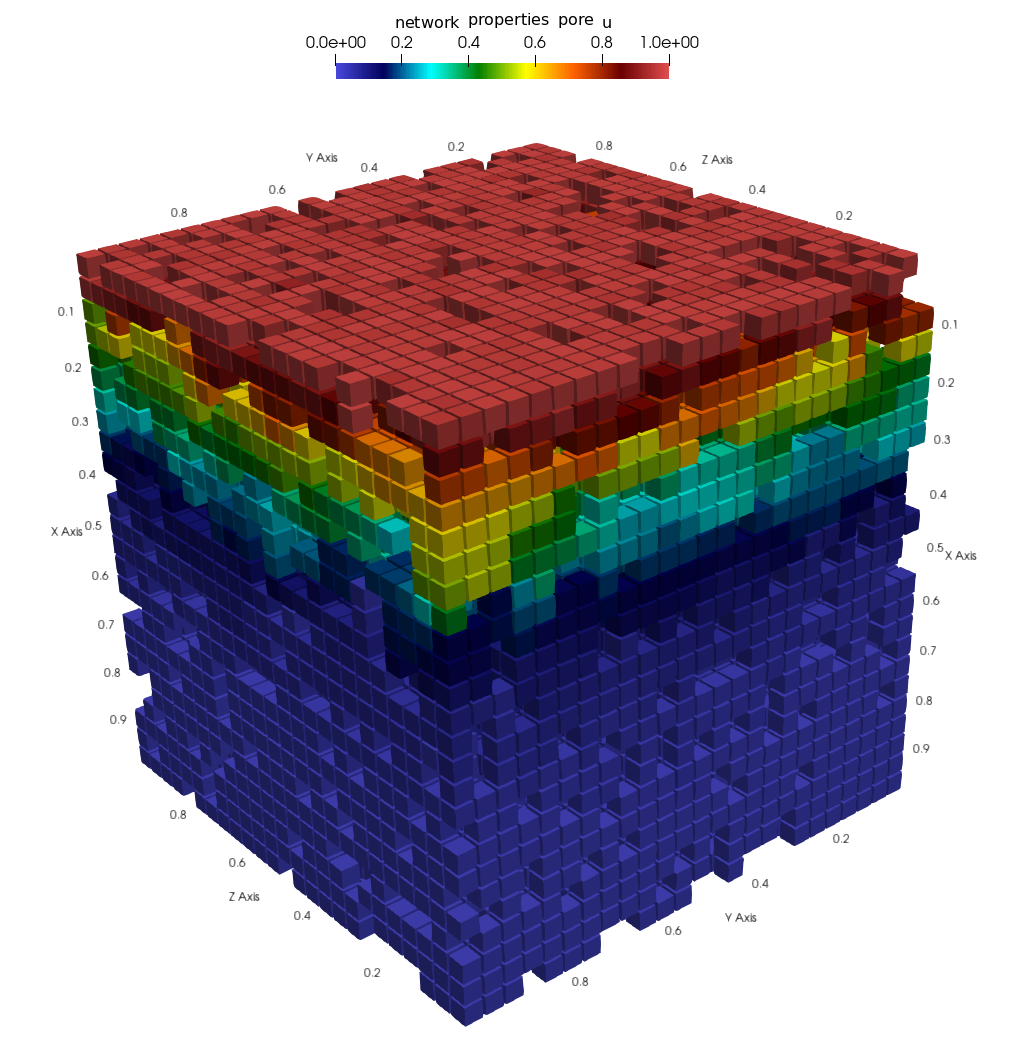
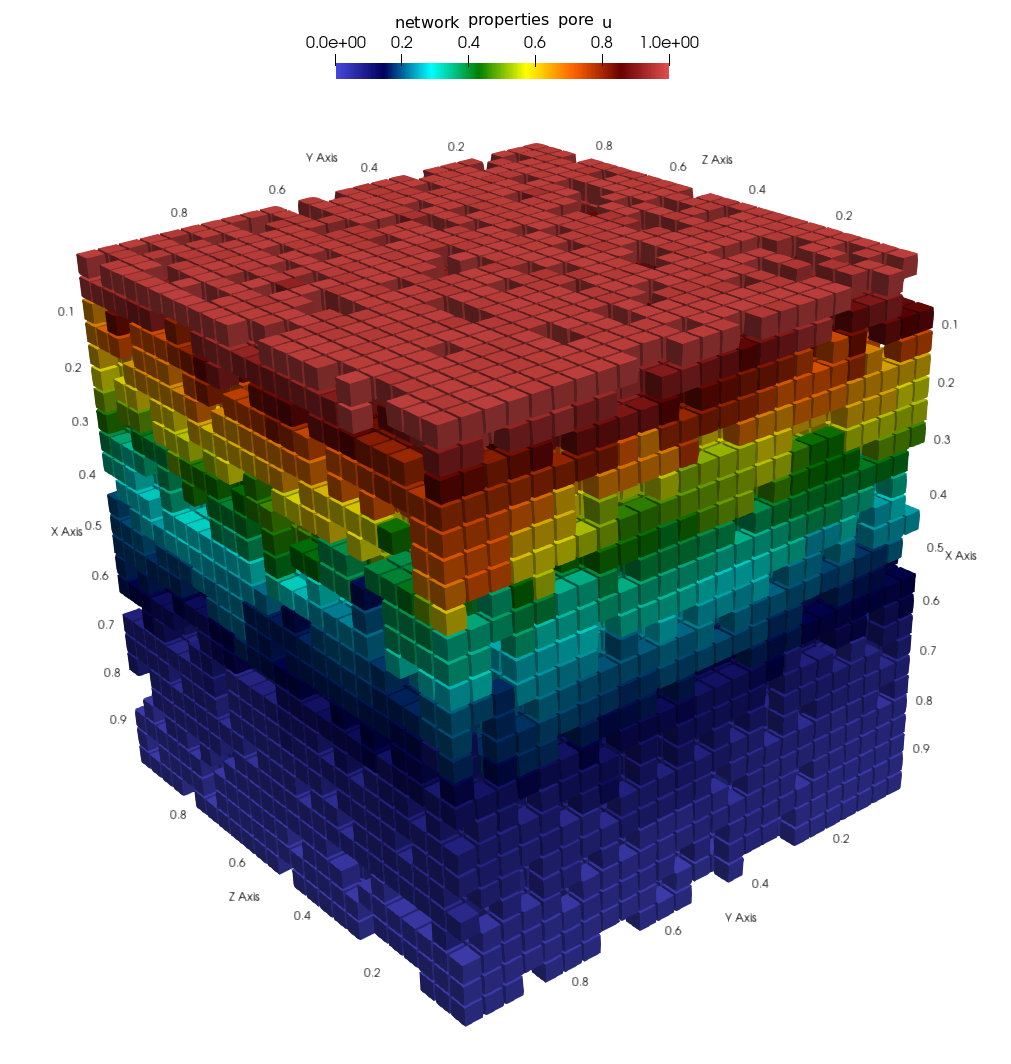
(b) Multiscale solution: $u_{ms}^{5}$, $u_{ms}^{20}$ and $u_{ms}^{50}$

Figure 8: Numerical solution for Network-2.

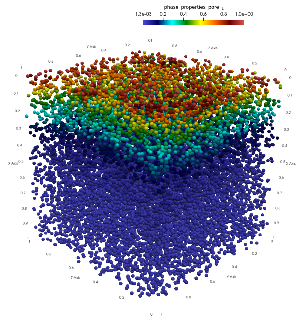
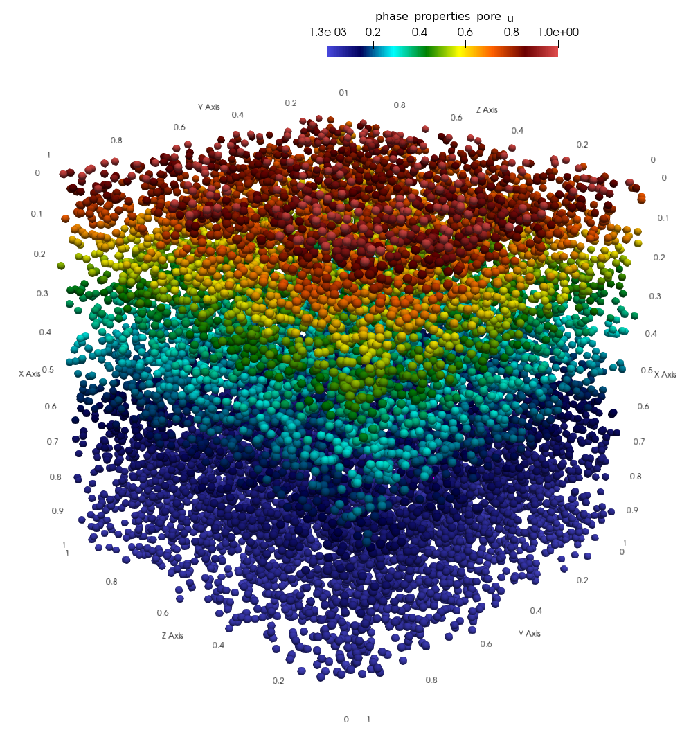
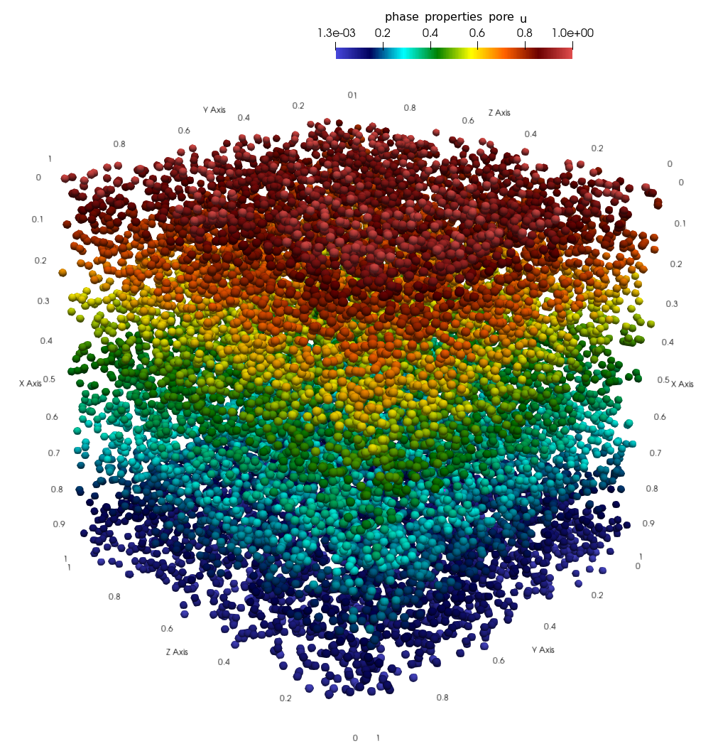
(a) Fine-scale solution: $u^{5}$, $u^{20}$ and $u^{50}$

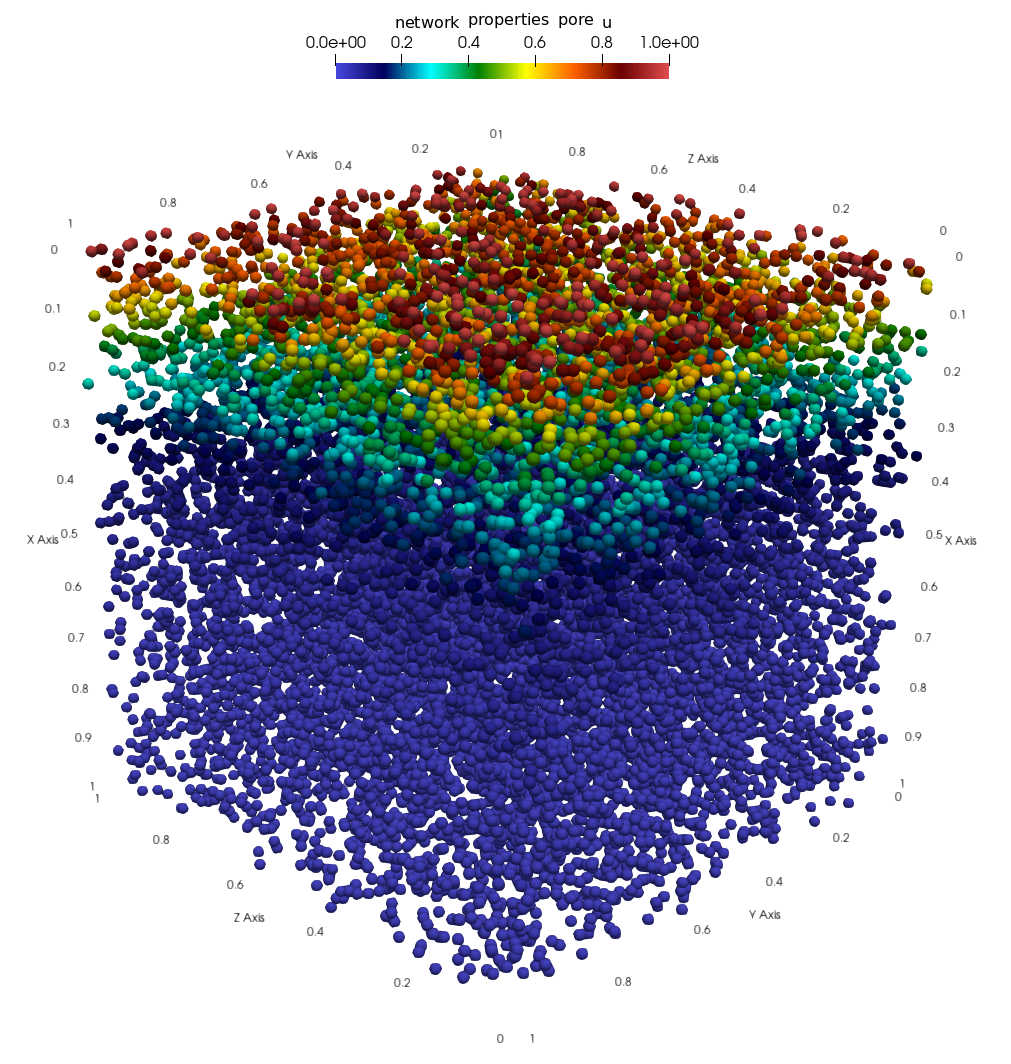
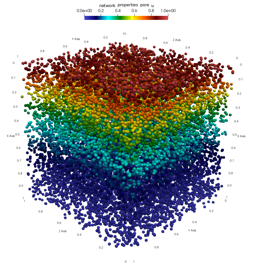
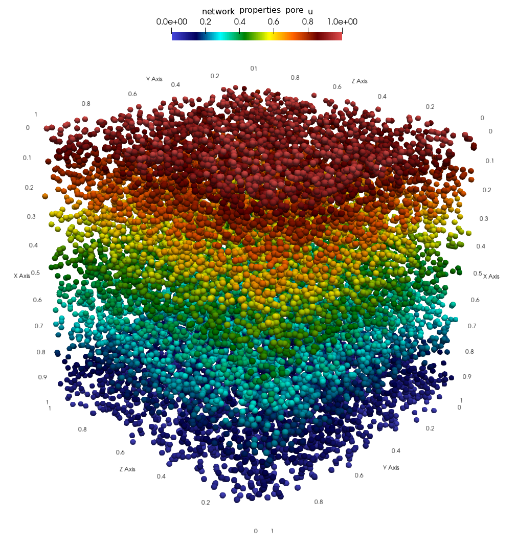
(b) Multiscale solution: $u_{ms}^{5}$, $u_{ms}^{20}$ and $u_{ms}^{50}$

Figure 9: Numerical solution for Network-3.

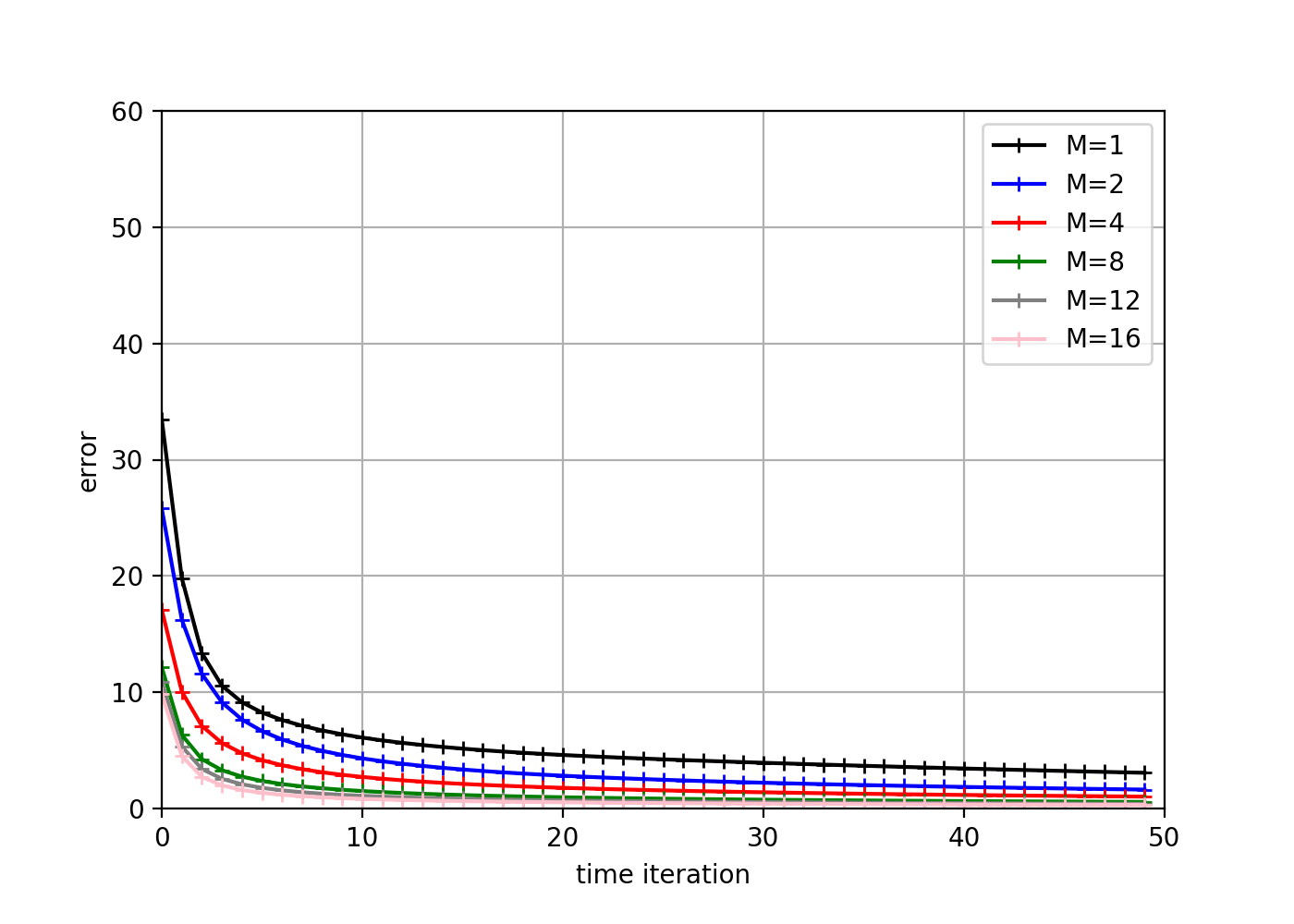
(a) Network-1

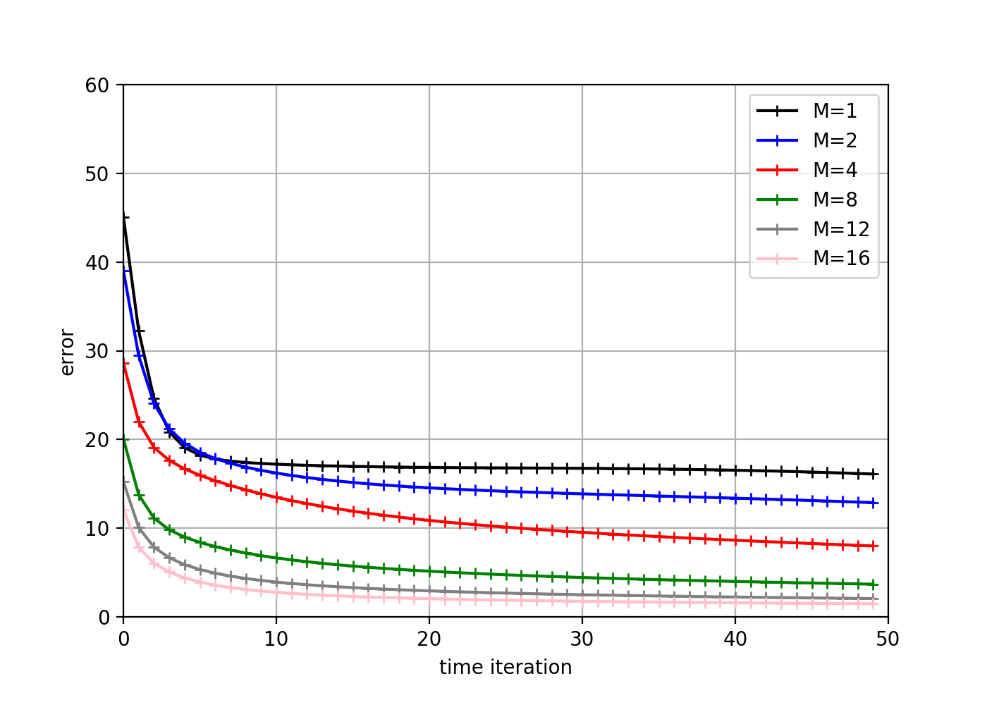
(b) Network-2

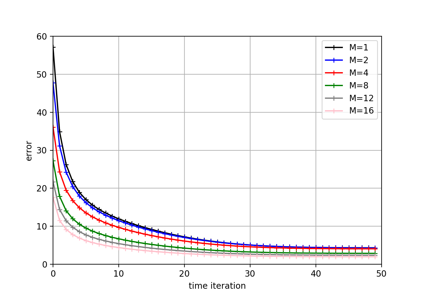
(c) Network-3

Figure 10: Dynamic of error for Network-1, Network-2 and Network-3

Nodes	M	Network-1	Network-2	Network-3
216	1	3.071	16.102	4.329
432	2	1.628	12.880	4.278
864	4	1.023	7.996	4.066
1728	8	0.410	3.688	2.868
2592	12	0.349	2.064	2.376
3456	16	0.207	1.479	1.976

Table 1: Numerical results. The number of unknowns on the fine-scale model is 15625 for Network 1, 12765 for Network-2, and 15625 for Network-3

We apply the presented multiscale method for each network and investigate accuracy for different number numbers of basis functions. The networks are embedded into domain ($\Omega=[0,1]\times[0,1]\times[0,1]$. We set zero source terms and set Dirichlet boundary conditions on top and bottom boundaries with one and zero values, respectively. The time used in simulation was $T=0.5$ (Network-1) and $T=50$ (Network-2 and 3) with 50 time steps. The coarse grid is $5\times 5\times 5$. In Figure 6, we represent eigenvectors corresponding to the first eight smallest eigenvalues for each network. Numerical implementation of the network model is performed based on the PETSc DMNetwork framework [35, 7, 5]. The basis functions are constructed using a generalized eigenvalue solver from SLEPc [48].

To compare the accuracy of the presented multiscale method, we use the relative $L_{2}$ error in percentage. The errors are calculated using the following formula on the fine grid:

$$e^{n}=\frac{||u^{n}-u_{ms}^{n}||_{L_{2}}}{||u^{n}||_{L_{2}}}\times 100\%,$$

where $n$ is the time layer, $u^{n}$ are the reference (fine grid) solution and $u_{ms}^{n}$ are the solution using the multiscale method. We use the corresponding fine-grid solution for each test problem as a reference solution.

In Figures 7,8, and 9, we depict the reference (fine grid) and multiscale solution for Network-1, Network-2, and Network-3, respectively. The simulation results are presented for three time layers $t_{5}$, $t_{20}$ and $t_{50}$ (from left to right). The reference solution is presented on the first row, and a multiscale solution using 16 multiscale basis functions on the second row. From the fine-scale solution, we observe a significant influence of the heterogeneity properties and network structure on the solution. The fine-scale network model leads to the system of equations with $DOF_{h}=15625$ for Network-1, $DOF_{h}=12765$ for Network-2 and $DOF_{h}=15625$ for Network-3. By the multiscale method, we reduce the size of the system to $DOF_{H}=1728$ for eight multiscale basis functions with 0.4 %, 2.06 %, and 2.8 % of errors for Network-1, Network-2, and Network-3. We have $DOF_{H}=3456$ for 16 multiscale basis functions with 0.2 %, 1.4 % and 1.9 % of errors for Network-1, Network-2 and Network-3.

In Table 1, we present errors at the final time for Network-1, Network-2, and Network-3. We have good accuracy for the multiscale method with a sufficient number of multiscale basis functions. For example, we have 3.07 %, 16.1 %, and 4.3 % of relative error for one basis function per local domain for Network-1, Network-2, and Network-3, respectively. When we use eight multiscale basis functions, errors reduce to 0.4 %, 2.06 %, and 2.8 %. We observe a significant influence of the network structure on the multiscale method solution, where for the first structure network, we obtain a better accuracy for a multiscale method using a smaller number of basis functions. Unstructured networks give a more significant error using one basis function, but accurate approximation can be performed with a larger number of basis functions. The dynamic of the errors is presented in Figure 10 for Network-1, Network-2, and Network-3. We observe that the errors reduce over time and give an accurate solution for structured and unstructured networks.

5 Conclusion

We considered a time-dependent model on structured and random networks. The time approximation was performed using an implicit scheme. The stability of the semi-discrete and discrete networks was presented. The multiscale method for the network model was developed and analyzed for network models. The proposed approach is based on the generalized multiscale finite element method. To find a multiscale basis function, we solve local eigenvalue problems in sub-networks. Convergence analysis of the proposed method was presented for semi-discrete and discrete network models with stability estimates. Numerical results were presented for structured and random heterogeneous networks to confirm the theory.

References

- [1] Morgan Görtz, Gustav Kettil, Axel Målqvist, Andreas Mark, and Fredrik Edelvik. A numerical multiscale method for fiber networks. arXiv preprint arXiv:2004.13348, 2020.
- [2] Martin J Blunt. Flow in porous media—pore-network models and multiphase flow. Current opinion in colloid & interface science, 6(3):197–207, 2001.
- [3] Oleg Iliev, Raytcho Lazarov, and Joerg Willems. Fast numerical upscaling of heat equation for fibrous materials. Computing and visualization in science, 13(6):275, 2010.
- [4] Morgan Görtz, Fredrik Hellman, and Axel Målqvist. Iterative solution of spatial network models by subspace decomposition. arXiv preprint arXiv:2207.07488, 2022.
- [5] Getnet Betrie, Hong Zhang, Barry F Smith, and Eugene Yan. A scalable river network simulator for extreme scale computers using the petsc library. In AGU Fall Meeting Abstracts, volume 2018, pages DI23A–07, 2018.
- [6] Shrirang Abhyankar, Getnet Betrie, Daniel Adrian Maldonado, Lois C Mcinnes, Barry Smith, and Hong Zhang. Petsc dmnetwork: A library for scalable network pde-based multiphysics simulations. ACM Transactions on Mathematical Software (TOMS), 46(1):1–24, 2020.
- [7] DANIEL A Maldonado, SHRIRANG Abhyankar, BARRY Smith, and HONG Zhang. Scalable multiphysics network simulation using petsc dmnetwork. Argonne National Laboratory: Lemont, IL, USA, 2017.
- [8] Jordan Jalving, Shrirang Abhyankar, Kibaek Kim, Mark Hereld, and Victor M Zavala. A graph-based computational framework for simulation and optimisation of coupled infrastructure networks. IET Generation, Transmission & Distribution, 11(12):3163–3176, 2017.
- [9] Rylee Sundermann, Shrirang G Abhyankar, Hong Zhang, Jung-Han Kimn, and Timothy M Hansen. Parallel primal-dual interior point method for the solution of dynamic optimal power flow. IET Generation, Transmission & Distribution, 17(4):811–820, 2023.
- [10] Rylee Sundermann. Efficient Numerical Optimization for Parallel Dynamic Optimal Power Flow Simulation Using Network Geometry. South Dakota State University, 2022.
- [11] Fabio Della Rossa, Carlo D’Angelo, Alfio Quarteroni, et al. A distributed model of traffic flows on extended regions. Networks Heterog. Media, 5(3):525–544, 2010.
- [12] Matt J Keeling and Ken TD Eames. Networks and epidemic models. Journal of the royal society interface, 2(4):295–307, 2005.
- [13] Johannes Reichold, Marco Stampanoni, Anna Lena Keller, Alfred Buck, Patrick Jenny, and Bruno Weber. Vascular graph model to simulate the cerebral blood flow in realistic vascular networks. Journal of Cerebral Blood Flow & Metabolism, 29(8):1429–1443, 2009.
- [14] Ettore Vidotto, Timo Koch, Tobias Koppl, Rainer Helmig, and Barbara Wohlmuth. Hybrid models for simulating blood flow in microvascular networks. Multiscale Modeling & Simulation, 17(3):1076–1102, 2019.
- [15] Enrique Sánchez-Palencia. Non-homogeneous media and vibration theory. Lecture Note in Physics, Springer-Verlag, 320:57–65, 1980.
- [16] Vasili Vasilievitch Jikov, Sergei M Kozlov, and Olga Arsenievna Oleinik. Homogenization of differential operators and integral functionals. Springer Science & Business Media, 2012.
- [17] Nikolai Sergeevich Bakhvalov and Grigory Panasenko. Homogenisation: averaging processes in periodic media: mathematical problems in the mechanics of composite materials, volume 36. Springer Science & Business Media, 2012.
- [18] Grégoire Allaire. Homogenization and two-scale convergence. SIAM Journal on Mathematical Analysis, 23(6):1482–1518, 1992.
- [19] Thomas Y Hou and Xiao-Hui Wu. A multiscale finite element method for elliptic problems in composite materials and porous media. Journal of computational physics, 134(1):169–189, 1997.
- [20] Yalchin Efendiev and Thomas Y Hou. Multiscale finite element methods: theory and applications, volume 4. Springer Science & Business Media, 2009.
- [21] Assyr Abdulle, E Weinan, Björn Engquist, and Eric Vanden-Eijnden. The heterogeneous multiscale method. Acta Numerica, 21:1–87, 2012.
- [22] Patrick Henning and Axel Målqvist. Localized orthogonal decomposition techniques for boundary value problems. SIAM Journal on Scientific Computing, 36(4):A1609–A1634, 2014.
- [23] Thomas JR Hughes, Gonzalo R Feijóo, Luca Mazzei, and Jean-Baptiste Quincy. The variational multiscale method—a paradigm for computational mechanics. Computer methods in applied mechanics and engineering, 166(1-2):3–24, 1998.
- [24] Yalchin Efendiev, Juan Galvis, and Xiao-Hui Wu. Multiscale finite element methods for high-contrast problems using local spectral basis functions. Journal of Computational Physics, 230(4):937–955, 2011.
- [25] Yalchin Efendiev, Juan Galvis, and Thomas Y Hou. Generalized multiscale finite element methods (gmsfem). Journal of computational physics, 251:116–135, 2013.
- [26] Ivan Lunati and Patrick Jenny. Multiscale finite-volume method for compressible multiphase flow in porous media. Journal of Computational Physics, 216(2):616–636, 2006.
- [27] Hadi Hajibeygi, Giuseppe Bonfigli, Marc Andre Hesse, and Patrick Jenny. Iterative multiscale finite-volume method. Journal of Computational Physics, 227(19):8604–8621, 2008.
- [28] Gustav Kettil, Axel Målqvist, Andreas Mark, Mats Fredlund, Kenneth Wester, and Fredrik Edelvik. Numerical upscaling of discrete network models. BIT Numerical Mathematics, 60:67–92, 2020.
- [29] Artem Kulachenko and Tetsu Uesaka. Direct simulations of fiber network deformation and failure. Mechanics of Materials, 51:1–14, 2012.
- [30] Jay Chu, Björn Engquist, Maša Prodanović, and Richard Tsai. A multiscale method coupling network and continuum models in porous media i: steady-state single phase flow. Multiscale Modeling & Simulation, 10(2):515–549, 2012.
- [31] Jay Chu, Björn Engquist, Maša Prodanović, and Richard Tsai. A multiscale method coupling network and continuum models in porous media ii—single-and two-phase flows. Advances in Applied Mathematics, Modeling, and Computational Science, pages 161–185, 2013.
- [32] Andrew T Barker, Chak S Lee, and Panayot S Vassilevski. Spectral upscaling for graph laplacian problems with application to reservoir simulation. SIAM Journal on Scientific Computing, 39(5):S323–S346, 2017.
- [33] Andrew T Barker, Stephan V Gelever, Chak S Lee, Sarah V Osborn, and Panayot S Vassilevski. Multilevel spectral coarsening for graph laplacian problems with application to reservoir simulation. SIAM Journal on Scientific Computing, 43(4):A2737–A2765, 2021.
- [34] Matthew T Balhoff, Sunil G Thomas, and Mary F Wheeler. Mortar coupling and upscaling of pore-scale models. Computational Geosciences, 12:15–27, 2008.
- [35] Satish Balay, Shrirang Abhyankar, Mark Adams, Jed Brown, Peter Brune, Kris Buschelman, Lisandro Dalcin, Alp Dener, Victor Eijkhout, W Gropp, et al. Petsc users manual. 2019.
- [36] Jeff Gostick, Mahmoudreza Aghighi, James Hinebaugh, Tom Tranter, Michael A Hoeh, Harold Day, Brennan Spellacy, Mostafa H Sharqawy, Aimy Bazylak, Alan Burns, et al. Openpnm: a pore network modeling package. Computing in Science & Engineering, 18(4):60–74, 2016.
- [37] Amir Raoof and S Majid Hassanizadeh. A new method for generating pore-network models of porous media. Transport in porous media, 81:391–407, 2010.
- [38] Jean Gallier. Spectral theory of unsigned and signed graphs. applications to graph clustering: a survey, 2016.
- [39] Martin J. Blunt. Flow in porous media — pore-network models and multiphase flow. Current Opinion in Colloid & Interface Science, 6(3):197–207, 2001.
- [40] Moritz Hauck and Axel Målqvist. Super-localization of spatial network models. arXiv preprint arXiv:2210.07860, 2022.
- [41] Alexander A Samarskii. The theory of difference schemes, volume 240. CRC Press, 2001.
- [42] Petr N Vabishchevich. Additive operator-difference schemes. In Additive Operator-Difference Schemes. de Gruyter, 2013.
- [43] Maria Vasilyeva. Efficient decoupling schemes for multiscale multicontinuum problems in fractured porous media. Journal of Computational Physics, 487:112134, 2023.
- [44] Splitting schemes for poroelasticity and thermoelasticity problems. Computers & Mathematics with Applications, 67(12):2185–2198, 2014.
- [45] Yalchin Efendiev and Maria Vasilyeva. Multiscale model reduction for shale gas transport in fractured media. Computational Geosciences, 20:953–973, 2016.
- [46] Eric T Chung, Yalchin Efendiev, Guanglian Li, and Maria Vasilyeva. Generalized multiscale finite element methods for problems in perforated heterogeneous domains. Applicable Analysis, 95(10):2254–2279, 2016.
- [47] Eduardo Abreu, Ciro Díaz, and Juan Galvis. A convergence analysis of generalized multiscale finite element methods. Journal of Computational Physics, 396:303–324, 2019.
- [48] Vicente Hernandez, Jose E Roman, and Vicente Vidal. Slepc: A scalable and flexible toolkit for the solution of eigenvalue problems. ACM Transactions on Mathematical Software (TOMS), 31(3):351–362, 2005.
- [49] Shubin Fu, Eric Chung, and Lina Zhao. Generalized multiscale finite element method for highly heterogeneous compressible flow. Multiscale Modeling & Simulation, 20(4):1437–1467, 2022.
- [50] Xiaofei Guan, Lijian Jiang, Yajun Wang, and Zihao Yang. A coupling generalized multiscale finite element method for coupled thermomechanical problems. arXiv preprint arXiv:2302.01674, 2023.
- [51] Leonardo A Poveda, Shubin Fu, Eric T Chung, and Lina Zhao. Convergence of the cem-gmsfem for compressible flow in highly heterogeneous media. arXiv preprint arXiv:2303.17157, 2023.
- [52] Jens M Melenk and Ivo Babuška. The partition of unity finite element method: basic theory and applications. Computer methods in applied mechanics and engineering, 139(1-4):289–314, 1996.