Efficient Solution of Point-Line Absolute Pose

Abstract

We revisit certain problems of pose estimation based on 3D–2D correspondences between features which may be points or lines. Specifically, we address the two previously-studied minimal problems of estimating camera extrinsics from $p\in\{1,2\}$ point–point correspondences and $l=3-p$ line–line correspondences. To the best of our knowledge, all of the previously-known practical solutions to these problems required computing the roots of degree $\geq 4$ (univariate) polynomials when $p=2$, or degree $\geq 8$ polynomials when $p=1.$ We describe and implement two elementary solutions which reduce the degrees of the needed polynomials from $4$ to $2$ and from $8$ to $4$, respectively. We show experimentally that the resulting solvers are numerically stable and fast: when compared to the previous state-of-the art, we may obtain nearly an order of magnitude speedup. The code is available at https://github.com/petrhruby97/efficient_absolute

1 Introduction

1.1 Motivation

The problem of registering images to a known 3D coordinate system plays a crucial role in applications such as visual localization [26], autonomous driving [12], and augmented reality [28], as well as in general paradigms like SLAM [15] and SfM [27]. Robust estimators based on RANSAC [11], or one of its many refinements [24, 3], are among the most successful tools for solving these problems. Such an estimator traditionally relies on a minimal P3P solver [23, 8, 13, 16] to efficiently hypothesize poses from putative matches between 3D and 2D points.

The literature on P3P and other purely point-based methods for absolute pose estimation is vast. Absolute pose estimation from non-point features such as lines [7, 25, 30, 5, 29, 2], point-line incidences [10], and affine correspondences [28], has received comparatively less attention, but remains an active research area. In particular, solutions relying on both points and lines are of increasing importance, due to the prevalence of both types of feature in man-made environments, as well as several recent advances in the components of 3D reconstruction systems responsible for line detection [21], matching [22], and bundle adjustment [19].

Figure 1: The P2P1L (Top) and P1P2L (Bottom) problems.

1.2 Contribution

In this paper, we revisit the two minimal problems of absolute pose estimation that combine both points and lines: the Perspective-2-Point-1-Line Problem (or P2P1L, Section 2.1), and the Perspective-1-Point-2-Line Problem (P1P2L, Section 2.2.) See Figure 1 for illustrations.

In contrast to the purely point or line based minimal problems P3P and P3L, we observe that the existing solutions for the “mixed cases” considered here are suboptimal from both a theoretical and practical point of view. Consequently, we develop novel solutions to both problems, which optimally exploit their underlying algebraic structure, and exhibit comparable or better performance than the state of the art on simulated and real data—see Section 3. On the other hand, these solvers are simple to implement, and no knowledge of mathematics beyond elementary algebra is needed to understand them.

To provide further context for our work, we include the following quotation from [25]: Although we do not theoretically prove that our solutions are of the lowest possible degrees, we believe so because of the following argument. The best existing solutions for pose estimation using three points and three lines use 4th and 8th degree solutions respectively. Since mixed cases are in the middle, our solutions for (2 points, 1 line) and (1 point, 2 lines) cases use 4th and 8th degree solutions respectively. Recently, it was shown using Galois theory that the solutions that use the lowest possible degrees are the optimal ones [[20]].

Contrary to the informal reasoning presented above, we claim that the existing solutions to the mixed point–line cases are not optimal. As far as we know, the only support for this claim appearing in the literature prior to our work occurs in [9, §3]. This previous work showed, on the basis of Galois group computation, that the P2P1L and P1P2L problems decompose into simpler subproblems. However, this theoretical observation was not accompanied by a practical solution method for either problem. In this paper, we rectify the situation by devising practical solvers for both problems that incorporate these recent insights.

To complete our discussion of what makes a solution algebraically optimal, we recall one proposal of such a notion from work of Nistér et al. [20]. In this work, a restricted class of algorithms $\mathcal{P}_{n}$ is considered for each natural number $n\geq 1$: an algorithm in $\mathcal{P}_{n}$ consists of a finite sequence of steps, each of which extracts the roots of some polynomial equation $p(x)=0$, with either $p(x)=x^{m}-a$ (where $a\in\mathbb{Q}$ and $\deg(p)=m$ can be arbitrary), or with $\deg(p)\leq n$ and the coefficients of $p$ belonging to a field containing $\mathbb{Q}$ and any previously-computed roots. In this setting, a solution is optimal if it leads to solving a polynomial system of the lowest possible degree. Our proposed solutions immediately establish that P2P1L is $\mathcal{P}_{2}$-solvable and P1P2L is $\mathcal{P}_{4}$-solvable. It should be of little surprise that P2P1L is not $\mathcal{P}_{1}$-solvable; therefore, we may say that our solution to P2P1L is algebraically optimal. On the other hand, the problem P1P2L is also $\mathcal{P}_{3}$-solvable. This is because any quartic equation can be solved by the standard method which reduces the problem to computing the roots of the associated resolvent cubic. Thus, our solution, which computes the roots of a quartic with this same method, is also algebraically optimal in the sense of [20]. The same observation, of course, holds for the classical quartic-based methods for solving P3P. Alternative P3P solvers that directly employ a cubic [23, 8], despite being superior in practical terms, are not distinguished by the complexity classes $\mathcal{P}_{n}.$ Table 1 provides a summary of the algebraic complexities, based on the Galois groups computed in [9, §3].

problem	P3P	P2P1L	P1P2L	P3L
class	$\mathcal{P}_{3}$	$\mathcal{P}_{2}$	$\mathcal{P}_{3}$	$\mathcal{P}_{8}$

Table 1: For each minimal absolute pose problem with points and line features, the class of polynomial root finding algorithms $\mathcal{P}_{n}$ that solve the problem with $n$ as small as possible [20, §2.1].

1.3 Related work

The first solutions to P2P1L and P1P2L were presented by Ramalingam et al. [25], reducing the problems to computing the roots of polynomials of degree $4$ and $8$ via careful choices of special reference frames in the world and image. Although we obtain polynomials of lower degree, these special reference frames are also an ingredient in our approach.

In work subsequent to [25], it was observed that both of these problems could be solved using the E3Q3 solver [17]. This is a highly optimized method for computing the points where three quadric surfaces in $\mathbb{R}^{3}$ intersect. Typically, there are $2^{3}=8$ such points, by Bézout’s theorem; however, EQ3Q also handles degenerate cases where the number of solutions may drop. In the follow-up work [30], a stabilization scheme for E3Q3 was applied to these problems, and experimentally shown to be more accurate than the solvers in [25]. Efficient solvers for both problems based on this stabilized E3Q3 are implemented in PoseLib [18].

The idea of using Galois groups to study minimal problems originates from [20]. The main takeaway from this paper is that a problem with $n$ solutions whose Galois group is the full symmetric group $S_{n}$ cannot be solved by an algorithm in $\mathcal{P}_{n-1}.$ In the other direction, the main takeaway from [9] is that if the Galois group is contained in the wreath product $S_{n_{1}}\wr S_{n_{2}},$ where $n=n_{1}n_{2},$ then the problem can be solved with an algorithm in $\mathcal{P}_{\max(n_{1},n_{2})}.$ A recent work using such an insight to guide the more efficient solution of a relative pose estimation problem may be found in [14].

2 Minimal solvers

In this section, we introduce our algebraically optimal solutions to the P2P1L and P1P2L problems. These problems are depicted in Figure 1. As revealed by the Galois group computed in [9, §3], the problem P2P1L can be reduced to computing the roots of a quadratic equation, and the problem P1P2L can be reduced to a quartic equation. In Sections 2.1 and 2.2, we turn these insights into explicit solutions to the P2P1L and P12PL problems, respectively. These solutions work generically—they are valid outside of a measure-zero subset of the space of input point-point/line-line correspondences. In Section 2.3, we describe a method that stabilizes the P1P2L solver of Section 2.2 in a common but non-generic case. Finally, Section 2.4 for a discussion when the point-line configuration is coplanar.

&

Figure 2: Special reference frame for P2P1L. Camera frame $\mathcal{C}_{0}$ is transformed to $\mathcal{C}_{1}$, world frame $\mathcal{W}_{0}$ to $\mathcal{W}_{1}$. See text for details.

2.1 P2P1L

Here, we provide the algebraically optimal solution to the P2P1L problem. We mostly follow the notation of [25].

Problem Statement: Consider $P_{1}^{0},P_{2}^{0}\in\mathbb{R}^{3}$, two 3D points, and their 2D projections under an unknown calibrated camera. Consider also a 3D line spanned by points $L_{3}^{0},L_{4}^{0}\in\mathbb{R}^{3}$ and its projection. The goal is to recover the unknown camera matrix, whose center we denote by $C^{0}$.

Our first step is to rigidly transform the input into the special reference frame introduced in [25]. Transforming to this special frame simplifies the equations and helps to reveal the algebraically optimal solution. Section 2 illustrates the input reference frame $\mathcal{C}_{0}$ / $\mathcal{W}_{0}$ (top), and the special frame $\mathcal{C}_{1}$ / $\mathcal{W}_{1}$ (bottom), which are related as follows:

• In the world frame $\mathcal{W}_{1}$, the 3D points take the form

  $$P_{1}=\begin{pmatrix}0&0&0\end{pmatrix}^{T},\quad P_{2}=\begin{pmatrix}X_{2}&0&0\end{pmatrix}^{T},$$ (1)

  and the 3D line is spanned by two points of the form

  $$L_{3}=\begin{pmatrix}X_{3}&Y_{3}&0\end{pmatrix}^{T},\quad L_{4}=\begin{pmatrix}X_{4}&Y_{4}&Z_{4}\end{pmatrix}^{T}.$$ (2)

• To find the transformation $\mathcal{W}_{0}\rightarrow\mathcal{W}_{1}$, we set P_1 = (0 0 0 )^T, P_2 = (∥P10- P22∥0 0 )^T, L_3 = (X3Y30 )^T, w/   X_3 = (L_3^0-P_1)^T P2-P1∥P2-P1∥, Y_3 = ∥L_3^0 - P_1 - X_3⋅P2-P1∥P2-P1∥ ∥. We transform the rays $\overrightarrow{P_{1}^{0}P_{2}^{0}}$ and $\overrightarrow{P_{1}^{0}L_{3}^{0}}$ to $\overrightarrow{P_{1}P_{2}}$ and $\overrightarrow{P_{1}L_{3}},$ respectively, via suitable translation and rotation.

• In the camera frame, the camera center is fixed at

  $$C=\begin{pmatrix}0&0&-1\end{pmatrix}^{T},$$ (3)

  the 2D points are projections of points of the form

  $$D_{1}=\begin{pmatrix}a_{1}&b_{1}&0\end{pmatrix}^{T},\quad D_{2}=\begin{pmatrix}a_{2}&b_{2}&0\end{pmatrix}^{T},$$ (4)

  and the 2D line is the projection of $\overline{D_{3}D_{4}},$ where

  $$D_{3}=\begin{pmatrix}0&0&0\end{pmatrix}^{T},\quad D_{4}=\begin{pmatrix}1&0&0\end{pmatrix}^{T}.$$ (5)

• To find the transformation $\mathcal{C}_{0}\rightarrow\mathcal{C}_{1}$, let $D_{3}^{0}$ and $D_{4}^{0}$ be the homogeneous coordinates of two distinct points along the given line. Independently of $C^{0},$ we may rigidly transform the rays $d_{3}:=\overrightarrow{C^{0}D_{3}^{0}}$, and $d_{4}:=\overrightarrow{C^{0}D_{3}^{0}}$ to $\overrightarrow{CD_{3}}$ and $\overrightarrow{CD_{4}},$ by suitable rotation and translation.

Let us now write $R=(R_{ij})_{1\leq i,j\leq 3}$, $T=(T_{i})_{1\leq i\leq 3}$ for the unknown camera pose in this special reference frame. Our projection constraints can then be written as

$$(D_{i}-C)\times(RP_{i}+T)=0,\quad i\in\{1,2\},$$ (6)

$$(D_{3}\times D_{4})^{T}(RL_{i}+T)=0,\quad i\in\{3,4\}.$$ (7)

This gives a system of equations in $12$ unknowns. However, in what follows, we consider a system of equations in a smaller set of unknowns, namely

$$\mathbf{x}^{T}=\begin{pmatrix}R_{11}&R_{21}&R_{31}&R_{22}&R_{23}&T_{1}&T_{2}&T_{3}\end{pmatrix}.$$ (8)

The entries of $\mathbf{x}$ are constrained by

$$R_{11}^{2}+R_{21}^{2}+R_{31}^{2}=R_{21}^{2}+R_{22}^{2}+R_{23}^{2} =1.$$ (9)

Thus, the entries of $\mathbf{x}$ specify a translation vector and a partially-filled rotation matrix, which can be uniquely completed to a rotation matrix using the formulae

$$\begin{pmatrix}R_{12}\\ R_{13}\\ R_{32}\\ R_{33}\end{pmatrix}=(R_{22}^{2}+R_{23}^{2})^{-1}\cdot\begin{pmatrix}-R_{11}R_{21}R_{22}+R_{23}R_{31}\\ -R_{11}R_{21}R_{23}-R_{22}R_{31}\\ -R_{21}R_{22}R_{31}-R_{11}R_{23}\\ -R_{21}R_{23}R_{31}+R_{11}R_{22}\end{pmatrix},$$ (10)

subject to the genericity condition $R_{22}^{2}+R_{23}^{2}\neq 0$, ie. when $R$ is not a rotation in the $xz$-plane. Hence, we focus on recovering the entries of $\mathbf{x}$. From 2 out of the 3 redundant constraints from (6) together with (7), we obtain linear constraints on $\mathbf{x}$ ([25, eq. (4)–(5)]),

$$A\mathbf{x} =\mathbf{b},\quad\text{where}$$

$$A =\begin{pmatrix}0&0&0&0&0&-b_{1}&a_{1}&0\\ 0&0&0&0&0&0&-1&b_{1}\\ -b_{2}X_{2}&a_{2}X_{2}&0&0&0&-b_{2}&a_{2}&0\\ 0&-X_{2}&b_{2}X_{2}&0&0&0&-1&b_{2}\\ 0&X_{3}&0&Y_{3}&0&0&1&0\\ 0&X_{4}&0&Y_{4}&Z_{4}&0&1&0\end{pmatrix},$$

$$\mathbf{b}^{T} =\begin{pmatrix}0&-b_{1}&0&-b_{2}&0&0\end{pmatrix}.$$ (11)

We may use these linear equations to solve for the translation $T$ in terms of $R$ and the problem data as follows:

$$T_{1} =a_{1}B,\quad T_{2}=b_{1}B,\quad T_{3}=-1+B,\quad\text{where}$$

$$B =\displaystyle\frac{X_{2}(a_{2}R_{21}-b_{2}R_{11})}{b_{2}a_{1}-b_{1}a_{2}}.$$ (12)

Moreover, from (2.1) we may use $R_{11}$ and $R_{21}$, to express the remaining entries of $R$ as

$$R_{31} =\displaystyle\frac{(a_{1}-a_{2})R_{21}+(b_{2}-b_{1})R_{11})}{b_{2}a_{1}-b_{1}a_{2}},$$

$$R_{22} =\displaystyle\frac{b_{1}b_{2}X_{2}R_{11}+(b_{1}a_{2}X_{2}-b_{1}a_{2}X_{2}-b_{2}a_{1}X_{3})R_{21}}{Y_{3}(b_{2}a_{1}-b_{1}a_{2})},$$

$$R_{23} =\displaystyle\frac{b_{1}b_{2}X_{2}(Y_{3}-Y_{4})R_{11}}{Y_{3}Z_{4}(b_{2}a_{1}-b_{1}a_{2})}$$

$$+\left(\displaystyle\frac{X_{3}Y_{4}-X_{4}Y_{3}}{Y_{3}Z_{4}}+\displaystyle\frac{b_{2}a_{1}X_{3}Y_{4}-b_{1}a_{2}X_{2}Y_{3}}{Y_{3}Z_{4}(b_{2}a_{1}-b_{1}a_{2})}\right)R_{21}.$$ (13)

Substituting (2.1) into (9), we obtain two bivariate quadratic constraints in $R_{11}$ and $R_{21}$. In matrix form,

$$\begin{pmatrix}c_{1}&c_{2}&c_{3}\\ d_{1}&d_{2}&d_{3}\end{pmatrix}\cdot\begin{pmatrix}R_{11}^{2}\\ R_{11}R_{21}\\ R_{21}^{2}\end{pmatrix}=\begin{pmatrix}1\\ 1\end{pmatrix},$$ (14)

where the coefficients $c_{1},c_{2},c_{3},d_{1},d_{2},d_{3}$ are rational functions of the problem data. Applying the change of variables

$$u=R_{11}^{2},\quad v=R_{21}/R_{11},$$ (15)

and subtracting the two equations in (14), we obtain

$$(c_{1}-d_{1})u+(c_{2}-d_{2})uv+(c_{3}-d_{3})uv^{2}=0.$$

Assuming $u\neq 0,$ we therefore have the univariate quadratic equation in $v$

$$(c_{1}-d_{1})+(c_{2}-d_{2})v+(c_{3}-d_{3})v^{2}=0.$$ (16)

If $v$ is one of the roots of (16), we may recover a corresponding value for $u$ using one of the equations in (14), eg.

$$u=(c_{1}+c_{2}v+c_{3}v^{2})^{-1},\quad\text{or}\quad u=(d_{1}+d_{2}v+d_{3}v^{2})^{-1}.$$ (17)

To summarize, we provide the outline of steps for solving the P2P1L absolute pose problem in Figure 3.

1. Transform data in world and camera frames to the special reference frames satisfying (1), (2), (3), (4), (5).

2. Compute up to 2 solutions in $v$ to the quadratic (16).

3. For each root $v$ in step (2), recover a corresponding value of $u$ using either of the linear expressions in (46).

4. Recover up to $4$ solutions in $\{R_{11},R_{21}\}$ using (15).

5. Recover $R$ and $T$ using (2.1), (2.1), (10).

6. Reverse the transformation applied in step (1).

Figure 3: Generic P2P1L solver. See Sec. 2.1 for details.

Algebraically, the nontrivial steps in Figure 3 are the second and fourth, which require solving a univariate quadratic equation and computing square roots, respectively.

&

Figure 4: Special reference frame for P1P2L. Camera frame $\mathcal{C}_{0}$ is transformed to $\mathcal{C}_{1}$, world frame $\mathcal{W}_{0}$ to $\mathcal{W}_{1}$. See text for details.

2.2 P1P2L

Here, we provide the algebraically optimal solution to the P1P2L problem. We mostly follow the notation of [25].

Problem Statement: Let us consider a 3D point $P_{1}^{0}\in\mathbb{R}^{3}$, and its homogeneous 2D projection $D_{1}\in\mathbb{R}^{3}$ under an unknown calibrated camera matrix. Let us also consider two 3D lines—the first spanned by points $L_{1},L_{2}\in\mathbb{R}^{3}$, and the second one is spanned by $L_{3},L_{4}\in\mathbb{R}^{3}$—and both of their corresponding projections. Our task is to recover the camera matrix from the given point-point correspondence and line-line correspondences.

Much like the P2P1L solver, our P1P2L solver begins by transforming the input data into a special reference frame, as illustrated in Section 2. Specifically,

• In the world frame, the 3D point takes the form

  $$P_{1}=\begin{pmatrix}0&0&0\end{pmatrix}^{T}.$$ (18)

  The first line is spanned by points

  $$L_{1}=\begin{pmatrix}X_{1}&Y_{1}&Z_{1}\end{pmatrix}^{T},\quad L_{2}=\begin{pmatrix}X_{2}&Y_{2}&Z_{2}\end{pmatrix}^{T},$$ (19)

  and the second line is spanned by points

  $$L_{3}=\begin{pmatrix}X_{3}&Y_{3}&Z_{3}\end{pmatrix}^{T},\quad L_{4}=\begin{pmatrix}X_{4}&Y_{4}&Z_{4}\end{pmatrix}^{T}.$$ (20)

• For $\mathcal{W}_{0}\rightarrow\mathcal{W}_{1}$, we simply translate $P_{1}^{0}$ to $P_{1}$.

• The world frame may still be rotated freely. We may use the strategy of Section 2.3, which makes the solver stable for a larger class of non-coplanar scenes. However, if $P_{1},\overline{L_{1}L_{2}},$ and $\overline{L_{3}L_{4}}$ are coplanar, no rotation is recommended.

• In the camera frame, the camera center is fixed at

  $$C=\begin{pmatrix}0&0&-1\end{pmatrix}^{T}.$$ (21)

  The image point is the projection of a point of the form

  $$D_{1}=\begin{pmatrix}a_{1}&b_{1}&0\end{pmatrix}^{T},$$ (22)

  the first line in the image is the projection of a line spanned by points of the form

  $$D_{2}=\begin{pmatrix}a_{2}&0&0\end{pmatrix}^{T},\quad D_{3}=\begin{pmatrix}0&0&0\end{pmatrix}^{T},$$ (23)

  and the second line in the image is the projection of a line spanned by points of the form

  $$D_{4}=\begin{pmatrix}a_{4}&b_{4}&0\end{pmatrix}^{T},\quad D_{5}=\begin{pmatrix}a_{5}&b_{5}&0\end{pmatrix}^{T}.$$ (24)

• The homogeneous coordinates of the lines in the camera frame are $n_{1}=d_{2}\times d_{3}$, $n_{2}=d_{4}\times d_{5}$, where the rays $d_{2}\neq d_{3},d_{4}\neq d_{5}$ to meet the lines in distinct points.

• To find the transformation $\mathcal{C}_{0}\rightarrow\mathcal{C}_{1}$, we define d_12 = n_1 ×n_2,  D_2^0 = C^0 + d2d2Td12,  D_3^0 = C^0 + d_3, D_2 = (tan(cos-1(d2Td12)) 0 0 )^T,  D_3 = (0 0 0 )^T, and, independently of $C^{0}$, rigidly transform the rays $d_{2}:=\overrightarrow{C^{0}D_{2}^{0}}$ and $d_{3}:=\overrightarrow{C^{0}D_{3}^{0}}$ to $\overrightarrow{C^{0}D_{2}^{0}}$ and $\overrightarrow{CD_{3}}.$

In the special reference frame, we now write the pose as $(R_{ij})_{1\leq i,j\leq 3}$, $(T_{i})_{1\leq i\leq 3}$. The projection constraints can be formulated as:

$$(D_{1}-C)\times(RP_{1}+T)=0,$$ (25)

$$(D_{2}\times D_{3})^{T}(RL_{i}+T)=0,i\in\{1,2\},$$ (26)

$$(D_{4}\times D_{5})^{T}(RL_{i}+T)=0,i\in\{3,4\}.$$ (27)

Analagously to (2.1), we have a system of linear equations $A\mathbf{x}=\mathbf{b},$ obtained by picking 2 out of the 3 redundant constraints from (25) together with (26), (27) , where now (cf. [25, eq. 7–8])

$$A =\begin{pmatrix}0&0&0&0&0&0&-b_{1}&a_{1}&0\\ 0&0&0&0&0&0&0&-1&b_{1}\\ 0&0&X_{1}&Y_{1}&Y_{1}&Z_{1}&0&1&0\\ 0&0&X_{2}&Y_{2}&Y_{2}&Z_{2}&0&1&0\\ -b_{4}X_{3}&-b_{4}Y_{3}&a_{4}X_{3}&a_{4}Y_{3}&a_{4}Y_{3}&a_{4}Z_{3}&-b_{4}&a_{4}&0\\ -b_{4}X_{4}&-b_{4}Z_{4}&a_{4}X_{4}&a_{4}Y_{4}&a_{4}Y_{4}&a_{4}Z_{4}&-b_{4}&a_{4}&0\\ \end{pmatrix},$$

$$\mathbf{x} =\begin{pmatrix}R_{11}&R_{12}&R_{13}&R_{21}&R_{22}&R_{23}&T_{1}&T_{2}&T_{3}\end{pmatrix}^{T},$$

$$\mathbf{b} =\begin{pmatrix}0&-b_{1}&0&0&0&0\end{pmatrix}^{T}.$$

Solving for translation as in (2.1), we have

$$\begin{split}T_{1}&=\frac{a_{1}}{b_{1}}(-R_{21}X_{1}-R_{22}Y_{1}-R_{23}Z_{1}),\\ T_{2}&=-R_{21}X_{1}-R_{22}Y_{1}-R_{23}Z_{1},\\ T_{3}&=-1+\frac{1}{b_{1}}(-R_{21}X_{1}-R_{22}Y_{1}-R_{23}Z_{1}).\end{split}$$ (28)

Furthermore, we express $R_{23}$ from the fourth equation as

$$R_{23}=\frac{1}{Z_{1}-Z_{2}}(R_{21}(X_{2}-X_{1})+R_{22}(Y_{2}-Y_{1})),$$ (29)

and we solve for $R_{11}$, $R_{12}$ using the last two equations.

Now, we can express $R_{23}$, $T_{2}$, $T_{1}$, $R_{12}$, $R_{11}$ as linear combinations of $R_{13}$, $R_{21}$, $R_{22}$ in the following form:

$$\begin{split}R_{23}&=c_{1}R_{21}+c_{2}R_{22},\\ T_{2}&=c_{3}R_{21}+c_{4}R_{22},\\ T_{1}&=c_{5}R_{21}+c_{6}R_{22},\\ R_{12}&=c_{7}R_{13}+c_{8}R_{21}+c_{9}R_{22},\\ R_{11}&=c_{10}R_{13}+c_{11}R_{21}+c_{12}R_{22}.\end{split}$$ (30)

The non-linear internal constraints imposed on the elements of $R$ have the form:

$$\begin{split}R_{11}^{2}+R_{12}^{2}+R_{13}^{2}&=1,\\ R_{21}^{2}+R_{22}^{2}+R_{23}^{2}&=1,\\ R_{11}R_{21}+R_{12}R_{22}+R_{13}R_{23}&=0.\end{split}$$ (31)

We substitute (30) into (31), obtaining equations of the form

$$\begin{pmatrix}d_{1}&d_{2}&d_{3}&d_{4}&d_{5}&d_{6}\end{pmatrix}\nu(R) =1,$$ (32)

$$\begin{pmatrix}0&0&0&d_{7}&d_{8}&d_{9}\end{pmatrix}\nu(R) =1,$$ (33)

$$\begin{pmatrix}0&d_{10}&d_{11}&d_{12}&d_{13}&d_{14}\end{pmatrix}\nu(R) =0,$$ (34)

where

$$\nu(R)=\begin{pmatrix}R_{13}^{2}&R_{13}R_{21}&R_{13}R_{22}&R_{21}^{2}R_{21}R_{22}&R_{22}^{2}\end{pmatrix}^{T}.$$ (35)

We express $R_{13}$ from (34) as

$$R_{13}=-\frac{d_{12}R_{21}^{2}+d_{13}R_{21}R_{22}+d_{14}R_{22}^{2}}{d_{10}R_{21}+d_{11}R_{22}}.$$ (36)

Substituting (36) into (32), we obtain

$$d_{1}\frac{(d_{12}R_{21}^{2}+d_{13}R_{21}R_{22}+d_{14}R_{22}^{2})^{2}}{(d_{10}R_{21}+d_{11}R_{22})^{2}}\,-$$

$$d_{2}\frac{d_{12}R_{21}^{3}+d_{13}R_{21}^{2}R_{22}+d_{14}R_{21}R_{22}^{2}}{d_{10}R_{21}+d_{11}R_{22}}\,-$$

$$d_{3}\frac{d_{12}R_{21}^{2}R_{22}+d_{13}R_{21}R_{22}^{2}+d_{14}R_{22}^{3}}{d_{10}R_{21}+d_{11}R_{22}}\,+$$

$$d_{4}R_{21}^{2}+d_{5}R_{21}R_{22}+d_{6}R_{22}^{2}=1.$$ (37)

Subtracting (33) from (37),

$$d_{1}\frac{(d_{12}R_{21}^{2}+d_{13}R_{21}R_{22}+d_{14}R_{22}^{2})^{2}}{(d_{10}R_{21}+d_{11}R_{22})^{2}}\,-$$

$$d_{2}\frac{d_{12}R_{21}^{3}+d_{13}R_{21}^{2}R_{22}+d_{14}R_{21}R_{22}^{2}}{d_{10}R_{21}+d_{11}R_{22}}\,-$$

$$d_{3}\frac{d_{12}R_{21}^{2}R_{22}+d_{13}R_{21}R_{22}^{2}+d_{14}R_{22}^{3}}{d_{10}R_{21}+d_{11}R_{22}}\,+$$

$$(d_{4}-d_{7})R_{21}^{2}+(d_{5}-d_{8})R_{21}R_{22}+(d_{6}-d_{9})R_{22}^{2}=0.$$ (38)

We then clear denominators in (38), multiplying by $(d_{10}R_{21}+d_{11}R_{22})^{2}$ to get a polynomial equation

$$\begin{split}&d_{1}(d_{12}R_{21}^{2}+d_{13}R_{21}R_{22}+d_{14}R_{22}^{2})^{2}\,-\\ \bigg{(}\Big{(}&d_{2}(d_{12}R_{21}^{3}+d_{13}R_{21}^{2}R_{22}+d_{14}R_{21}R_{22}^{2})\,-\\ &d_{3}(d_{12}R_{21}^{2}R_{22}+d_{13}R_{21}R_{22}^{2}+d_{14}R_{22}^{3})\Big{)}\,\cdot\\ (&d_{10}R_{21}+d_{11}R_{22})+((d_{4}-d_{7})R_{21}^{2}+\\ (&d_{5}-d_{8})R_{21}R_{22}\,+(d_{6}-d_{9})R_{22}^{2})\bigg{)}\cdot\\ (&d_{10}R_{21}+d_{11}R_{22})=0.\end{split}$$ (39)

Upon expanding equation (39), we find that it takes the form

$$\alpha_{1}R_{21}^{4}+\alpha_{2}R_{21}^{3}R_{22}+\alpha_{3}R_{21}^{2}R_{22}^{2}+\alpha_{4}R_{21}R_{22}^{3}+\alpha_{5}2R_{22}^{4}=0$$ (40)

Similarly to (16), we divide (40) by $R_{22}^{4}$ and define a new variable $v=\frac{R_{21}}{R_{22}}$, and thereby deduce the univariate quartic

$$\alpha_{1}v^{4}+\alpha_{2}v^{3}+\alpha_{3}v^{2}+\alpha_{4}v+\alpha_{5}=0.$$ (41)

After solving for $v$, we can solve for $R_{21},R_{22}$ using (33), and for the other equations using (34), and (30).

To summarize, we provide the outline of steps for solving the P1P2L absolute pose problem in Figure 5. Algebraically, the nontrivial steps in Figure 5 are second and third, which require solving a univariate quartic equation and computing square roots, respectively.

1. Transform data in world and camera frames to the special reference frames satisfying (18), (19), (20), (21), (22), (23), (24).

2. Compute up to 4 solutions in $v$ to the quartic (41).

3. For each root $v$ in step (2), recover $2$ solutions in $\{R_{21},R_{22}\}$ using $R_{21}=R_{22}v$ and (33).

4. Recover remaining coordinates for each solution using (34),(30).

5. Reverse the transformation applied in step (1).

Figure 5: Generic P1P2L solver. See Sec. 2.2 for details.

&

Figure 6: Stabilization of P1P2L solver. The frame is rotated to align the line $\overline{L_{1}L_{2}}$ with the z-axis. See Sec. 2.3 for details.

2.3 Stabilizing the P1P2L Solver

In this section, we outline a method to increase the stability of the P1P2L solver (Sec. 2.2).

Our proposed P1P2L solution faces a degeneracy when $Z_{1}-Z_{2}=0$, since this leads to a division by zero in equation (29). Furthermore, our observations indicate that the result of the solver is unstable if the value of $Z_{1}-Z_{2}$ is close to zero. Note, that this instability is specific to our solver and not inherent to the P1P2L problem.

This degeneracy may be interpreted geometrically as follows: the values of $Z_{1}$ and $Z_{2}$ are the last coordinates of the points $L_{1}$, $L_{2}$, which span the first 3D line. Therefore, the vector $L_{1}-L_{2}$ represents the direction of the line, and $Z_{1}-Z_{2}$ represents the last coordinate of this direction.

Since the special reference frame used in Section 2.2 is independent of the rotation of the world frame, we can remove the source of instability by rotating the world frame such that the first line $\overline{L_{1}L_{2}}$ aligns with the z-axis. See Section 2 for an illustration.

Generic	Mean R	Med. R	Mean T	Med. T
P1P2L no fix	0.00050	1.0e-14	0.00065	1.8e-13
P1P2L fix	9.0e-09	4.2e-15	3.4e-07	7.0e-14
P2P1L no fix	7.1e-11	1.4e-15	1.2e-09	2.1e-14
P2P1L fix	3.2e-09	2.6e-15	7.4e-08	4.3e-14
Coplanar	Mean R	Med. R	Mean T	Med. T
P1P2L no fix	0.00022	9.6e-15	0.00030	1.75e-13
P1P2L fix	1.1	0.79	1.2	0.96
P2P1L no fix	2.4	3.14	2.2	3.14
P2P1L fix	1.2e-12	4.0e-15	7.9e-11	6.3e-14

Table 2: The mean and median of the rot.(R) and tran.(T) errors over $1e5$ noiseless generic (top) and coplanar (bottom) samples. In radians. The best results are marked bold.

2.4 Resolving the coplanar case

In this section, we discuss the performance of the P2P1L (Sec. 2.1) and P1P2L (Sec. 2.2) solvers in the case, where all 3D points and 3D lines are coplanar.

P2P1L. The P2P1L solver presented in Sec. 2.1 (P2P1L no fix) is degenerate in coplanar situations, since then $Z_{4}=0$ (2), causing a division by zero issue in equation (2.1). To resolve this issue, we propose a modified solver (P2P1L fix), which handles the coplanar case. See SM A for a description of this modified solver.

P1P2L. The original version of the P1P2L solver (P1P2L no fix, Sec. 2.2) is able to handle the coplanar case. However, the stabilized P1P2L solver (P1P2L fix, Sec. 2.3) fails due to a degeneracy for coplanar input.

We conducted a synthetic experiment to evaluate the impact of the proposed stablization scheme. In this experiment, we used the same setting as in Section 3.1. The results, presented in Table 2 demonstrate that solvers P2P1L no fix and P1P2L fix achieve superior numerical stability in the generic case, while solvers P2P1L fix and P1P2L no fix handle the coplanar case. Since it is simple to detect the coplanar case, we recommend to use solvers P2P1L fix and P1P2L no fix in the coplanar case and solvers P2P1L no fix and P1P2L fix in the generic case.

3 Experiments

In this section, we experimentally compare the proposed solvers with the state-of-the-art methods, specifically 3Q3 [17] and Ramalingam [25]. For 3Q3, we employ the publicly available implementation from Poselib. As the implementation of Ramalingam is not publicly accessible, we have created our own implementation. Since it is not explicitly specified which method should be used for solving the linear equations, we compare with two variants: SVD and LU decomposition. All the solvers have been implemented in C++, and the experiments are conducted on a desktop computer with an AMD Ryzen 9 CPU with 3.9 GHz.

In Sec. 3.1, we provide an analysis of the numerical stability and runtime performance of the solvers on synthetic data. Subsequently, in Section 3.2, we present an evaluation of the solvers within the RANSAC scheme.

Figure 7: Stability test. Histogram of rotation (l.), and translation (r.) errors computed over $1e5$ noiseless samples.

Method	Mean	Med.	Min	Max
P2P1L Ours	313.8	324.9	230.8	3061.0
P2P1L 3Q3	1860.6	1909.9	1439.1	10102.1
P2P1L R.+S	8897.5	9491.2	5805.1	49984.1
P2P1L R.+L	4720.8	5239.5	2763.3	15362.6
P1P2L Ours	504.0	521.0	364.0	4554.4
P1P2L 3Q3	1967.1	2008.2	1483.9	12931.1

Table 3: Runtime The mean, median and max values of the runtime. In nanoseconds. Best values for each problem are bold.

Method	Mean R	Median R	Max R	Mean T	Median T	Max T
P2P1L Ours	5.3e-12	1.4e-15	1.2e-07	3.7e-10	2.1e-14	2.2e-05
P2P1L 3Q3	2.8e-05	6.5e-15	2.7	2.0e-05	1.2e-13	1.04
P2P1L Ramalingam (SVD)	4.9e-09	1.5e-14	0.00041	1.6e-07	2.7e-13	0.0099
P2P1L Ramalingam (LU)	4.7e-07	1.3e-14	0.040	2.3e-05	2.4e-13	0.10
PP1P2L Ours (fix 2)	1.2e-07	4.4e-15	0.010	2.0e-06	7.1e-14	0.13
P1P2L 3Q3	3.3e-05	7.2e-15	2.60	3.4e-05	1.5e-13	1.01

Table 4: The mean, median and max values of the rot.(R) and tran.(T) errors over $1e5$ noiseless samples. The best results are marked bold.

3.1 Synthetic experiments

In this section, we present an analysis of the numerical stability and runtime performance of the minimal solvers on synthetic data.

We generate instances of each minimal problem (either P2P1L or P1P2L), according to the following procedure:

• Rotation Matrix ($R$): An axis $v\in\mathbb{R}^{3}$ is sampled from the uniform distribution on the unit sphere, and an angle $\alpha$ is sampled from the normal distribution $\mathcal{N}(0,1).$ The rotation matrix $R$ is then constructed using the angle-axis formula, $R=I+\sin(\alpha)[v]_{\times}+(1-\cos(\alpha))[v]_{\times}^{2}$.

• Translation ($T$): The camera center $C$ is sampled uniformly at random from the unit sphere. The translation vector $T$ is computed as $T=-RC$.

• Point correspondence: A 3D point $X_{i}$ is sampled from the trivariate normal distribution with mean vector $\mu=[0,0,5]^{T}$ and standard deviation $\sigma=1$ in each component. The corresponding 2D point $D_{i}$ is obtained by projecting $X_{i}$ onto a pinhole camera with the pose $(R,T)$.

• Line correspondence: Two 3D points, $L_{i}$ and $L_{i+1}$, are sampled as described in the previous bullet-point. These points define the 3D line $L$. Two 2D points, $D_{i}$ and $D_{i+1}$, are obtained by sampling two points on the 3D line $L$ and projecting them onto the camera with the pose $(R,T)$.

In the case of P2P1L, two points and one line are sampled, while in the case of P1P2L, one point and two lines are sampled. Let $(R_{est},T_{est})$ be the pose obtained by the minimal solver. We measure the rotation error as the angle $\xi_{R}=\arccos((1+\operatorname{trace}(R_{est}^{T}R))/2)$. We calculate the translation error $\xi_{T}$ as $\xi_{T}=\frac{|T_{est}-T|}{|T|}$. The histograms of rotation errors ($\xi_{R}$) and translation errors ($\xi_{T}$) for all considered solvers are depicted in Figure 7. Furthermore, summary statistics including the median, mean, and maximum errors are provided in Table 4. The results indicate that all minimal solvers are stable. Our algebraically optimal solvers demonstrate superior stability compared to the previous solvers.

The runtime evaluation for all considered solvers is shown in Table. 3. Our P2P1L solver requires $313.8ns$ on average, which is about 6x faster than the 3Q3 solver [17]. Similarly, our P1P2L solver requires on average $504.0ns$, which is about 4x faster than the 3Q3 solver. These results show a significant speedup achieved by our solvers in comparison to the previous methods.

	P2P1L				P1P2L
Dataset	OUR	3Q3	Ram. SVD	Ram. LU	OUR	3Q3
Model House	7.72 (0.85x)	9.09 (1x)	20.69 (2.28x)	17.30 (1.90x)	8.06 (0.85x)	9.52 (1x)
Corridor	11.32 (0.91x)	12.46 (1x)	26.56 (2.13x)	23.54 (1.89x)	13.3 (0.90x)	14.76 (1x)
Merton I	35.93 (0.98x)	36.83 (1x)	77.96 (2.12x)	74.87 (2.03x)	28.85 (0.64x)	45.41 (1x)
Merton II	33.30 (0.97x)	34.27 (1x)	74.37 (2.17x)	71.35 (2.08x)	26.7 (0.67x)	39.64 (1x)
Merton III	24.04 (0.96x)	25.07 (1x)	52.07 (2.08x)	48.97 (1.95x)	10.91 (0.37x)	29.67 (1x)
Library	32.42 (0.97x)	33.31 (1x)	69.29 (2.08x)	66.23 (1.99x)	10.04 (0.28x)	35.98 (1x)
Wadham	39.60 (0.98x)	40.51 (1x)	86.10 (2.13x)	83.00 (2.05x)	22.96 (0.45x)	50.79 (1x)
Avg. Speed-up	0.94x	1x	2.14x	1.99x	0.59x	1x

Table 5: RANSAC timing, on Oxford Multi-view dataset [1], in milliseconds. Speed-up compared to the 3Q3 in the bracket.

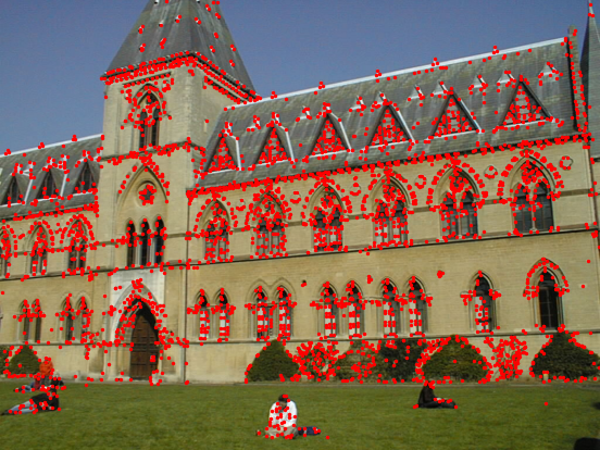
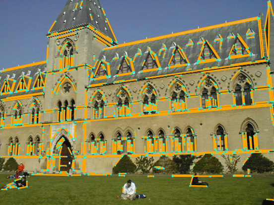
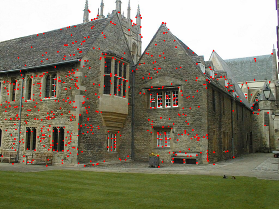
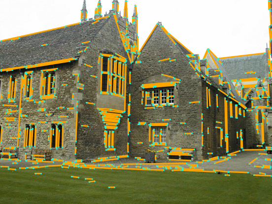
Figure 8: Example images of University Library (top) and Merton College III (bottom), from [1].

3.2 Experiments in RANSAC

Here, we provide an analysis of the minimal solvers within the RANSAC scheme [4], using the Oxford Multi-view Data [1]. This dataset includes a variety of indoor and outdoor scenes, some of which contain both point and line matches. An example of images from this dataset is illustrated in Figure 8.

We utilize the Poselib [18] implementation of LO-RANSAC [6]. In this implementation, local optimization is applied both when the new solution surpasses the currently best one and at the end of the entire procedure. The RANSAC parameters used include a maximum number of iterations set to 100000, a minimum number of iterations set to 1000, a success probability of 0.9999, and an inlier threshold of 1 pixel. To ensure a fair comparison between the solvers, we use a fixed random seed.

Since all the solvers are stable, we do not expect any significant difference in the estimated pose when using different solvers. Therefore, our primary focus is on comparing the runtime of the RANSAC scheme. The runtime comparison is presented in Table 5, which displays the average runtime for each scene in the Oxford multiview dataset and for each considered solver. Additionally, the table includes a speedup value compared to the 3Q3 solver of [18]. The results show that our solvers consistently outperform the 3Q3 [17] and Ramalingam [25] solvers in terms of runtime. However, there is a notable variation in the speed-up among the scenes, which ranges from 0.85 to 0.98 for the P2P1L problem and from 0.28 to 0.90 for the P1P2L solver. This variation can be attributed to the fact that different scenes require varying proportions of time spent by RANSAC on scoring hypothesized models and local optimization. The more time is dedicated to these tasks, the less significant speedup can be reached. In cases with fewer matches or a lower inlier ratio, more substantial speedups are possible.

The final pose estimation errors in RANSAC are shown in the Supplementary. As expected, the errors are the same for all solvers. This demonstrates that we can achieve improved runtimes without sacrificing any accuracy.

4 Conclusion

In revisiting absolute pose from mixed point-line corresopondences, we have developed new solvers, which have the merit of being both algebraically optimal and elementary in nature. Moreover, our solvers outperform the state-of-the-art in terms of both runtime and numerical stability. Despite the simplicity of many minimal absolute pose problems, our findings suggest that their continued investigation remains worthwhile. The code is available at https://github.com/petrhruby97/efficient_absolute

Acknowledgements: TD was supported by NSF DMS 2103310.

Supplementary Material

	P2P1L				P1P2L
Dataset	OUR	3Q3	Ram. SVD	Ram. LU	OUR	3Q3
Model House	0.251, 0.429	0.251, 0.429	0.251, 0.429	0.251, 0.429	0.251, 0.429	0.251, 0.429
Corridor	0.573, 0.580	0.573, 0.580	0.573, 0.580	0.573, 0.580	0.573, 0.580	0.573, 0.580
Merton I	0.005, 3.2e-4	0.005, 3.2e-4	0.005, 3.2e-4	0.005, 3.2e-4	0.005, 3.2e-4	0.005, 3.2e-4
Merton II	0.003, 4.6e-4	0.003, 4.6e-4	0.003, 4.6e-4	0.003, 4.6e-4	0.003, 4.6e-4	0.003, 4.6e-4
Merton III	0.007, 0.001	0.007, 0.001	0.007, 0.001	0.007, 0.001	0.007, 0.001	0.007, 0.001
Library	0.011, 0.002	0.011, 0.002	0.011, 0.002	0.011, 0.002	0.011, 0.002	0.011, 0.002
Wadham	0.007, 0.001	0.007, 0.001	0.007, 0.001	0.007, 0.001	0.007, 0.001	0.007, 0.001

Table 6: RANSAC error, on Oxford Multi-view dataset [1], in degrees. Every cell shows rotation and translation error.

Appendix A P2P1L in the coplanar case

Here, we describe the modified version of the P2P1L solver (Sec. 2.1) capable of handling the coplanar case. The input and output to this solver are the same as those of the original P2P1L solver.

The solver is identical to the original P2P1L solver until Equation (2.1). Then, we express values $R_{11},R_{31},R_{22}$ in terms of $R_{21},R_{23}$ as

$$\normalsize\begin{split}R_{11}=\frac{b_{2}a_{1}-b_{1}a_{2}}{b_{1}b_{2}X_{2}(Y_{3}-Y_{4})}\\ \cdot\Bigg{(}\bigg{(}Y_{3}X_{4}-Y_{4}X_{3}+\frac{b_{1}a_{2}(X_{2}Y_{3}-X_{1})}{b_{2}a_{1}-b_{1}a_{2}}\bigg{)}R_{21}\\ +Z_{4}Y_{3}R_{23}\Bigg{)}\\[5.0pt] R_{31}=\Bigg{(}\frac{b_{2}-b_{1}}{b_{1}b_{2}X_{2}(Y_{3}-Y_{4})}\bigg{(}Y_{3}X_{4}-Y_{4}X_{3}+\vphantom{\int_{1}^{2}}\\ \frac{b_{1}a_{2}(X_{2}Y_{3}-X_{1})}{b_{2}a_{1}-b_{1}a_{2}}\bigg{)}+\frac{a_{1}-a_{2}}{b_{2}a_{1}-b_{1}a_{2}}\Bigg{)}R_{21}\\ +\frac{(b_{2}-b_{1})Z_{4}Y_{3}}{b_{1}b_{2}X_{2}(Y_{3}-Y_{4})}R_{23},\\[5.0pt] R_{22}=\Bigg{(}\frac{1}{Y_{3}(Y_{3}-Y_{4})}\bigg{(}Y_{3}X_{4}-Y_{4}X_{3}\vphantom{\int_{1}^{2}}+\\ \frac{b_{1}a_{2}(X_{2}Y_{3}-X_{1})}{b_{2}a_{1}-b_{1}a_{2}}\bigg{)}-\frac{X_{3}}{Y_{3}}-\frac{b_{1}a_{2}X_{2}}{Y_{3}(b_{2}a_{1}-b_{1}a_{2})}\Bigg{)}R_{21}\\ +\frac{Z_{4}}{Y_{3}-Y_{4}}R_{23}\end{split}\normalsize$$ (42)

Then, we substitute (42) into (9), to obtain two bivariate quadratic constraints in $R_{21}$ and $R_{23}$. We can write them in matrix form as

$$\begin{pmatrix}c_{1}&c_{2}&c_{3}\\ d_{1}&d_{2}&d_{3}\end{pmatrix}\cdot\begin{pmatrix}R_{21}^{2}\\ R_{21}R_{23}\\ R_{23}^{2}\end{pmatrix}=\begin{pmatrix}1\\ 1\end{pmatrix},$$ (43)

where the coefficients $c_{1},c_{2},c_{3},d_{1},d_{2},d_{3}$ are rational functions of the problem data. Similarly to the original solver, we apply the change of variables

$$u=R_{21}^{2},\quad v=R_{23}/R_{21}$$ (44)

Subtracting the two equations in (43), we obtain

$$(c_{1}-d_{1})u+(c_{2}-d_{2})uv+(c_{3}-d_{3})uv^{2}=0.$$

Assuming $u\neq 0,$ we therefore have the univariate quadratic equation in $v$

$$(c_{1}-d_{1})+(c_{2}-d_{2})v+(c_{3}-d_{3})v^{2}=0.$$ (45)

We recover value $v$ as one of the roots of (45) and $u$ as

$$u=(c_{1}+c_{2}v+c_{3}v^{2})^{-1},\quad\text{or}\quad u=(d_{1}+d_{2}v+d_{3}v^{2})^{-1}.$$ (46)

After the values $u$, $v$ are recovered, we obtain $R_{21},R_{23}$ according to (43) and $R_{11},R_{31},R_{22}$ according to (42). The rest of the solver is identical to the original solver.

Appendix B Evaluation of the pose error.

In this section, we show the pose estimation errors obtained in the RANSAC experiment, following the same experimental setup as in Sec. 3.2. The results are presented in Table 6. As expected, the errors are the same for all solvers. This demonstrates that our solvers can achieve improved runtimes without sacrificing any accuracy.

References

- [1] Multi-view data, oxford visual geometry group. https://www.robots.ox.ac.uk/ vgg/data/mview/. Accessed: Nov 8 2023.
- Agostinho et al. [2023] Sérgio Agostinho, João Gomes, and Alessio Del Bue. CvxPnPL: A unified convex solution to the absolute pose estimation problem from point and line correspondences. Journal of Mathematical Imaging and Vision, 65(3):492–512, 2023.
- Barath and Matas [2022] Daniel Barath and Jiri Matas. Graph-cut RANSAC: local optimization on spatially coherent structures. IEEE Trans. Pattern Anal. Mach. Intell., 44(9):4961–4974, 2022.
- Bolles and Fischler [1981] Robert C. Bolles and Martin A. Fischler. A ransac-based approach to model fitting and its application to finding cylinders in range data. In Proceedings of the 7th International Joint Conference on Artificial Intelligence, IJCAI ’81, Vancouver, BC, Canada, August 24-28, 1981, pages 637–643. William Kaufmann, 1981.
- Chen [1991] Homer H. Chen. Pose determination from line-to-plane correspondences: Existence condition and closed-form solutions. IEEE Trans. Pattern Anal. Mach. Intell., 13(6):530–541, 1991.
- Chum et al. [2003] Ondrej Chum, Jiri Matas, and Josef Kittler. Locally optimized RANSAC. In Pattern Recognition, 25th DAGM Symposium, Magdeburg, Germany, September 10-12, 2003, Proceedings, pages 236–243. Springer, 2003.
- Dhome et al. [1989] Michel Dhome, Marc Richetin, Jean-Thierry Lapresté, and Gérard Rives. Determination of the attitude of 3d objects from a single perspective view. IEEE Trans. Pattern Anal. Mach. Intell., 11(12):1265–1278, 1989.
- Ding et al. [2023] Yaqing Ding, Jian Yang, Viktor Larsson, Carl Olsson, and Kalle Åström. Revisiting the P3P problem. In IEEE/CVF Conference on Computer Vision and Pattern Recognition, CVPR 2023, Vancouver, BC, Canada, June 17-24, 2023, pages 4872–4880. IEEE, 2023.
- Duff et al. [2022] Timothy Duff, Viktor Korotynskiy, Tomas Pajdla, and Margaret H. Regan. Galois/monodromy groups for decomposing minimal problems in 3d reconstruction. SIAM Journal on Applied Algebra and Geometry, 6(4):740–772, 2022.
- Fabbri et al. [2021] Ricardo Fabbri, Peter J. Giblin, and Benjamin B. Kimia. Camera pose estimation using first-order curve differential geometry. IEEE Trans. Pattern Anal. Mach. Intell., 43(10):3321–3332, 2021.
- Fischler and Bolles [1981] Martin A. Fischler and Robert C. Bolles. Random sample consensus: A paradigm for model fitting with applications to image analysis and automated cartography. Commun. ACM, 24(6):381–395, 1981.
- Häne et al. [2017] Christian Häne, Lionel Heng, Gim Hee Lee, Friedrich Fraundorfer, Paul Furgale, Torsten Sattler, and Marc Pollefeys. 3d visual perception for self-driving cars using a multi-camera system: Calibration, mapping, localization, and obstacle detection. Image Vis. Comput., 68:14–27, 2017.
- Haralick et al. [1994] Robert M. Haralick, Chung-Nan Lee, Karsten Ottenberg, and Michael Nölle. Review and analysis of solutions of the three point perspective pose estimation problem. Int. J. Comput. Vis., 13(3):331–356, 1994.
- Hruby et al. [2023] Petr Hruby, Viktor Korotynskiy, Timothy Duff, Luke Oeding, Marc Pollefeys, Tomás Pajdla, and Viktor Larsson. Four-view geometry with unknown radial distortion. In IEEE/CVF Conference on Computer Vision and Pattern Recognition, CVPR 2023, Vancouver, BC, Canada, June 17-24, 2023, pages 8990–9000. IEEE, 2023.
- Hu et al. [2023] Xiaomei Hu, Luying Zhu, Ping Wang, Haili Yang, and Xuan Li. Improved ORB-SLAM2 mobile robot vision algorithm based on multiple feature fusion. IEEE Access, 11:100659–100671, 2023.
- Kneip et al. [2011] Laurent Kneip, Davide Scaramuzza, and Roland Siegwart. A novel parametrization of the perspective-three-point problem for a direct computation of absolute camera position and orientation. In The 24th IEEE Conference on Computer Vision and Pattern Recognition, CVPR 2011, Colorado Springs, CO, USA, 20-25 June 2011, pages 2969–2976. IEEE Computer Society, 2011.
- Kukelova et al. [2016] Zuzana Kukelova, Jan Heller, and Andrew W. Fitzgibbon. Efficient intersection of three quadrics and applications in computer vision. In 2016 IEEE Conference on Computer Vision and Pattern Recognition, CVPR 2016, Las Vegas, NV, USA, June 27-30, 2016, pages 1799–1808. IEEE Computer Society, 2016.
- Larsson and contributors [2020] Viktor Larsson and contributors. PoseLib - Minimal Solvers for Camera Pose Estimation, 2020.
- Liu et al. [2023] Shaohui Liu, Yifan Yu, Rémi Pautrat, Marc Pollefeys, and Viktor Larsson. 3d line mapping revisited. In IEEE/CVF Conference on Computer Vision and Pattern Recognition, CVPR 2023, Vancouver, BC, Canada, June 17-24, 2023, pages 21445–21455. IEEE, 2023.
- Nistér et al. [2007] David Nistér, Richard I. Hartley, and Henrik Stewénius. Using galois theory to prove structure from motion algorithms are optimal. In 2007 IEEE Computer Society Conference on Computer Vision and Pattern Recognition (CVPR 2007), 18-23 June 2007, Minneapolis, Minnesota, USA. IEEE Computer Society, 2007.
- Pautrat et al. [2023a] Rémi Pautrat, Daniel Barath, Viktor Larsson, Martin R. Oswald, and Marc Pollefeys. Deeplsd: Line segment detection and refinement with deep image gradients. In IEEE/CVF Conference on Computer Vision and Pattern Recognition, CVPR 2023, Vancouver, BC, Canada, June 17-24, 2023, pages 17327–17336. IEEE, 2023a.
- Pautrat et al. [2023b] Rémi Pautrat, Iago Suárez, Yifan Yu, Marc Pollefeys, and Viktor Larsson. Gluestick: Robust image matching by sticking points and lines together. In Proceedings of the IEEE/CVF International Conference on Computer Vision, pages 9706–9716, 2023b.
- Persson and Nordberg [2018] Mikael Persson and Klas Nordberg. Lambda twist: An accurate fast robust perspective three point (P3P) solver. In Computer Vision - ECCV 2018 - 15th European Conference, Munich, Germany, September 8-14, 2018, Proceedings, Part IV, pages 334–349. Springer, 2018.
- Raguram et al. [2013] Rahul Raguram, Ondrej Chum, Marc Pollefeys, Jiri Matas, and Jan-Michael Frahm. USAC: A universal framework for random sample consensus. IEEE Trans. Pattern Anal. Mach. Intell., 35(8):2022–2038, 2013.
- Ramalingam et al. [2011] Srikumar Ramalingam, Sofien Bouaziz, and Peter F. Sturm. Pose estimation using both points and lines for geo-localization. In IEEE International Conference on Robotics and Automation, ICRA 2011, Shanghai, China, 9-13 May 2011, pages 4716–4723. IEEE, 2011.
- Sattler et al. [2017] Torsten Sattler, Bastian Leibe, and Leif Kobbelt. Efficient & effective prioritized matching for large-scale image-based localization. IEEE Trans. Pattern Anal. Mach. Intell., 39(9):1744–1756, 2017.
- Schönberger and Frahm [2016] Johannes L. Schönberger and Jan-Michael Frahm. Structure-from-motion revisited. In 2016 IEEE Conference on Computer Vision and Pattern Recognition, CVPR 2016, Las Vegas, NV, USA, June 27-30, 2016, pages 4104–4113. IEEE Computer Society, 2016.
- Ventura et al. [2014] Jonathan Ventura, Clemens Arth, Gerhard Reitmayr, and Dieter Schmalstieg. Global localization from monocular SLAM on a mobile phone. IEEE Trans. Vis. Comput. Graph., 20(4):531–539, 2014.
- Xu et al. [2017] Chi Xu, Lilian Zhang, Li Cheng, and Reinhard Koch. Pose estimation from line correspondences: A complete analysis and a series of solutions. IEEE Trans. Pattern Anal. Mach. Intell., 39(6):1209–1222, 2017.
- Zhou et al. [2018] Lipu Zhou, Jiamin Ye, and Michael Kaess. A stable algebraic camera pose estimation for minimal configurations of 2d/3d point and line correspondences. In Computer Vision - ACCV 2018 - 14th Asian Conference on Computer Vision, Perth, Australia, December 2-6, 2018, Revised Selected Papers, Part IV, pages 273–288. Springer, 2018.