Gauged Q-ball dark matter through a cosmological first-order phase transition

Abstract

As a new type of dynamical dark matter mechanism, we discuss the stability of the gauged Q-ball dark matter and its production mechanism through a cosmological first-order phase transition. This work delves into the study of gauged Q-ball dark matter generated during the cosmic phase transition. We demonstrate detailed discussions on the stability of gauged Q-balls to rigorously constrain their charge and mass ranges. Additionally, employing analytic approximations and the mapping method, we provide qualitative insights of gauged Q-ball. We establish an upper limit on the gauge coupling constant and give the relic density of stable gauged Q-ball dark matter formed during a first-order phase transition. Furthermore, we discuss potential observational signatures or constraints of gauged Q-ball dark matter, including astronomical observations and gravitational wave signals.

1 Introduction

Exploring the nature of dark matter (DM) is one of the central issues in (astro)particle physics and cosmology Bertone:2016nfn . So far, there are no expected signals of conventional DM candidates like Weakly Interacting Massive Particles (WIMPs) in the DM direct detection and collider search experiments Boveia:2022adi ; Boveia:2022syt ; Cooley:2022ufh . Then simple WIMP scenarios are strongly disfavored. There are a number of ways to save WIMP scenarios. For example, DM may have substantial couplings only to the 3rd generation fermions Baek:2016lnv ; Baek:2017ykw ; Abe:2016wck , or dark sectors may consists of two or more stable DM species (see, for example, Khan:2023uii ). Or one can discard WIMP scenarios and consider other possibilities for DM productions and annihilations or decays in the early Universe. This status motivates us to study ultralight or ultra heavy DM candidate (for reviews, see Refs. Baer:2014eja ; Lin:2019uvt ).

Solitons produced in the early Universe are natural candidates of heavy DM (see, for example, Baek:2013dwa for hidden sector monopole DM accompanied by stable spin-1 vector DM and massless dark radiation, and Ref. Derevianko:2013oaa for hunting for topological DM using atomic clocks). These solitons are specific field configurations which are classified into two classes, namely, the topological solitons and the non-topological solitions. Recently, as renaissance of the quark nuggets DM proposed by Witten Witten:1984rs , various new ideas on the non-topological solition DM are proposed, where the DM relic density can be produced by the dynamical process of cosmological first-order phase transition (FOPT), such as the Q-ball DM Krylov:2013qe ; Huang:2017kzu ; Jiang:2023qbm ; Hong:2020est . These new mechanisms can naturally avoid the unitarity problem for heavy DM Griest:1989wd . Dynamical DM mechanisms are specified by the DM penetration behavior into the bubble which depends on the DM mass and bubble wall velocity Baker:2019ndr ; Chway:2019kft .

There are extensive discussions on the non-topological solitons in a theory of complex scalar field with global $U(1)$ symmetry, proposed in Rosen:1968mfz and known as Q-balls Coleman:1985ki . And it is natural to study the Q-balls in the gauged case Coleman:1985ki ; Lee:1988ag ; Rosen:1968zwl ; Lee:1991bn ; Friedberg:1976me ; Arodz:2008nm ; Benci:2010cs ; Benci:2012fra ; Dzhunushaliev:2012zb , by promoting the global $U(1)$ symmetry to the local gauge $U(1)$ symmetry. For reviews of $U(1)$ gauged Q-balls, see Gulamov:2013cra ; Gulamov:2015fya ; Nugaev:2019vru . Q-balls have been proposed as a potential DM candidate in supersymmetric theories Kusenko:1997zq ; Kusenko:1997si . They can also explain the baryon asymmetry of the Universe Kasuya:2012mh . The gauged Q-ball DM in supersymmetry model has also been studied in several papers Hong:2017qvx ; Hong:2016ict . It is meaningful to search for other production mechanisms without supersymmetry of Q-ball or gauged Q-ball DM. In this paper, we study whether the $U(1)$ gauged Q-balls produced during cosmic phase transition could be a viable DM candidate. If the gauged Q-ball can be stable under certain circumstances, we still need some mechanism to (1) produce the charge asymmetry (i.e. locally produce lots of same charge particles to form Q-ball ) (2) and packet the same sign charges in the small size after overcoming the Coulomb repulsive interaction. For the first condition, the primordial charge asymmetry could be produced by some early Universe processes such as decays of heavier particles. Cosmological FOPT can naturally realize the second condition and can produce phase transition gravitational wave (GW) which can be detected by future GW experiments, such as LISA LISA:2017pwj , TianQin TianQin:2015yph ; Liang:2022ufy , Taiji Hu:2017mde , BBO Corbin:2005ny , DECIGO Seto:2001qf , and Ultimate-DECIGO Kudoh:2005as .

In this work, for the first time, we study the natural production mechanism of gauged Q-ball DM through a cosmological FOPT. The paper is organised as follows. We describe the basic model that can produce the gauged Q-balls and the numerical solutions of the Q-ball profiles in section 2. Basic properties and the stable parameter space of gauged Q-balls are discussed in section 3. Thin-wall approximation and the corresponding analytic evaluations are given in section 4. Phase transition dynamics in the Standard Model (SM) plus an extra singlet and the relic density of gauged Q-ball DM are elucidated in section 5. Signals and constraints of gauged Q-ball DM are given in section 6. Concise conclusions and discussions are given in section 7.

2 Gauged Q-ball

2.1 Friedberg-Lee-Sirlin–Maxwell model

In this work, we adopt the Friedberg-Lee-Sirlin two-component model Friedberg:1976me plus gauge component, which is called Friedberg-Lee-Sirlin-Maxwell (FLSM) model Lee:1991bn . This model and the corresponding stability of $U(1)$ gauged Q-ball have been discussed in Lee:1988ag ; Lee:1991bn ; Loiko:2019gwk ; Loiko:2022noq ; Kinach:2022jdx . We begin our discussions with the following Lagrangian density

$$\mathcal{L}=\left(D_{\mu}\phi\right)^{\dagger}\left(D^{\mu}\phi\right)+\frac{1}{2}\partial_{\mu}h\partial^{\mu}h-\frac{1}{4}\tilde{A}_{\mu\nu}\tilde{A}^{\mu\nu}-V(\phi,h)\,\,,$$ (1)

where the potential $V(\phi,h)$ reads

$$V(\phi,h)=\frac{\lambda_{\phi h}}{2}h^{2}|\phi|^{2}+\frac{\lambda_{h}}{4}\left(h^{2}-v_{0}^{2}\right)^{2}\,\,.$$ (2)

$\phi$ and $h$ are the complex scalar field and (real) Higgs field respectively. $D_{\mu}=\partial_{\mu}+i\tilde{g}\tilde{A}_{\mu}$ and $\tilde{A}_{\mu\nu}=\partial_{\mu}\tilde{A}_{\nu}-\partial_{\nu}\tilde{A}_{\mu}$ where $\tilde{A}_{\mu}$ is a dark $U(1)$ gauge field and $\tilde{g}$ is the corresponding gauge coupling constant. $\tilde{A}_{\mu}$ can be identified as the dark electromagnetic field. We fix the Higgs mass $m_{h}=125~{}\mathrm{GeV}$ and vacuum expectation value $v_{0}=246~{}\mathrm{GeV}$ at zero temperature then $\lambda_{h}=m_{h}^{2}/(2v_{0}^{2})\approx 0.13$. The complex scalar $\phi$ gains mass through the portal coupling with the Higgs. In the true vacuum, $m_{\phi}=\sqrt{\frac{\lambda_{\phi h}}{2}}v_{0}$. We assume $\lambda_{\phi h}>0$, and thus the Lagrangian density is symmetric under the dark $U(1)$ symmetry which remains unbroken when the Universe goes through the electroweak phase transition. The local $U(1)$ gauge symmetry leads to the conserved current,

$$J_{\mu}=i\left(\phi^{\dagger}\overleftrightarrow{\partial}_{\mu}\phi+2i\tilde{g}\tilde{A}_{\mu}|\phi|^{2}\right)\,\,,$$ (3)

and the corresponding conserved charge,

$$Q=\int d^{3}xJ^{0}\,\,.$$ (4)

Once the gauged Q-balls are formed in this FLSM model, one could consider a coherent configuration of $\phi$, $h$, and $\tilde{A}_{\mu}$ at a given charge $Q$. The lowest energy state will have no “magnetic field” so the space component $\tilde{A}_{i}=0$ Lee:1988ag ; Lee:1991bn . We assume spherical symmetry for the lowest energy configuration. Scaling away the physical dimensions, we introduce dimensionless field variables $\mathcal{A},\Phi$, and $\mathcal{H}$ defined in the convention of Ref. Lee:1991bn .

$$\tilde{A}_{t}(r)=v_{0}\frac{\tilde{g}}{\sqrt{2\lambda_{h}}}\mathcal{\mathcal{A}}(\rho),\quad\phi(r)=\frac{v_{0}}{\sqrt{2}}\Phi(\rho)e^{-i\omega t},\quad h(r)=v_{0}\mathcal{H}(\rho)\,\,,$$ (5)

where $\rho\equiv\sqrt{2\lambda_{h}}v_{0}r=m_{h}r$. The Lagrangian, with the substitution of the field variables defined above, becomes

$$L= -4\pi\frac{v_{0}}{\sqrt{2\lambda_{h}}}\int d\rho\rho^{2}\left[\frac{1}{2}\left(\nu-\alpha^{2}\mathcal{A}\right)^{2}\Phi^{2}-\frac{1}{8}\left(\mathcal{H}^{2}-1\right)^{2}-\frac{k^{2}}{2}\mathcal{H}^{2}\Phi^{2}-\frac{1}{2}\left(\partial_{\rho}\Phi\right)^{2}\right.$$ (6)

$$\left.-\frac{1}{2}\left(\partial_{\rho}\mathcal{H}\right)^{2}+\frac{\alpha^{2}}{2}\left(\partial_{\rho}\mathcal{A}\right)^{2}\right],$$

where $\alpha\equiv\frac{|\tilde{g}|}{\sqrt{2\lambda_{h}}},k\equiv\frac{\sqrt{\lambda_{\phi h}}}{2\sqrt{\lambda_{h}}}=\frac{m_{\phi}}{m_{h}}$, and $\nu\equiv\frac{\omega}{\sqrt{2\lambda_{h}}v_{0}}$. By varying $L$ with respect to $\mathcal{A},\Phi$, and $\mathcal{H}$, we find the equations of motion (EoM) for the three fields,

$$\frac{1}{\rho^{2}}\partial_{\rho}\left(\rho^{2}\partial_{\rho}\mathcal{A}\right)+(\nu-\alpha^{2}\mathcal{A})\Phi^{2}=0\,\,,$$ (7)

$$\frac{1}{\rho^{2}}\partial_{\rho}\left(\rho^{2}\partial_{\rho}\Phi\right)+\left[(\nu-\alpha^{2}\mathcal{A})^{2}-k^{2}\mathcal{H}^{2}\right]\Phi=0\,\,,$$ (8)

and

$$\frac{1}{\rho^{2}}\partial_{\rho}\left(\rho^{2}\partial_{\rho}\mathcal{H}\right)-k^{2}\mathcal{H}\Phi^{2}-\frac{1}{2}\mathcal{H}\left(\mathcal{H}^{2}-1\right)=0\,\,.$$ (9)

The total energy is given by

$$E=\frac{4\pi v_{0}}{\sqrt{2\lambda_{h}}}\int d\rho\rho^{2}\mathcal{E}\,\,,$$ (10)

where $\mathcal{E}=\frac{\alpha^{2}}{2}\left(\partial_{\rho}\mathcal{A}\right)^{2}+\frac{1}{2}\left(\partial_{\rho}\Phi\right)^{2}+\frac{1}{2}\left(\partial_{\rho}\mathcal{H}\right)^{2}+\frac{1}{2}\left[(\nu-\alpha^{2}\mathcal{A})^{2}+k^{2}\mathcal{H}^{2}\right]\Phi^{2}+\frac{1}{8}\left(\mathcal{H}^{2}-1\right)^{2}$. And the total charge is given by

$$Q=\frac{2\pi}{\lambda_{h}}\int d\rho\rho^{2}(\nu-\alpha^{2}\mathcal{A})\Phi^{2}\,\,.$$ (11)

From Eqs. (7) and (11) we see that

$$\frac{\lambda_{h}Q}{2\pi}=-\lim_{\rho\rightarrow\infty}4\pi\rho^{2}\partial_{\rho}\mathcal{A}\,\,.$$ (12)

Therefore we get, for large $\rho$, $\mathcal{A}\rightarrow\frac{\lambda_{h}Q}{2\pi\rho}$ or $\tilde{A}_{t}\rightarrow\frac{\tilde{g}Q}{4\pi r}$. Then Eq. (8) at large $\rho$ becomes

$$\frac{1}{\rho^{2}}\partial_{\rho}\left(\rho^{2}\partial_{\rho}\Phi\right)-\frac{2\nu\tilde{g}^{2}Q}{4\pi\rho}\Phi+\left(\nu^{2}-k^{2}\right)\Phi=0\,\,.$$ (13)

It has been shown in Ref. Gulamov:2015fya for $\nu<k$ that this equation at $\rho\rightarrow\infty$ has the solution of the form,

$$\Phi(\rho)=C_{U}\mathrm{e}^{-\sqrt{k^{2}-\nu^{2}}\rho}~{}U\left(1+\frac{\nu\tilde{g}^{2}Q}{4\pi\sqrt{k^{2}-\nu^{2}}},2,2\sqrt{k^{2}-\nu^{2}}\rho\right)\,\,,$$ (14)

where $C_{U}$ is a constant and $U(a,b,z)$ is the confluent hypergeometric function of the second kind. For $\sqrt{k^{2}-\nu^{2}}\rho\gg 1$ we get

$$\Phi(\rho)\sim\rho^{-1-\frac{\nu\tilde{g}^{2}Q}{4\pi\sqrt{k^{2}-\nu^{2}}}}\mathrm{e}^{-\sqrt{k^{2}-\nu^{2}}\rho}\,\,.$$ (15)

We can see that in the limit $\tilde{g}\rightarrow 0$ this form coincides with the nongauged global Q-ball, $\Phi(\rho)\sim\rho^{-1}\mathrm{e}^{-\sqrt{k^{2}-\nu^{2}}\rho}$. The difference is caused by taking into account the dark electromagnetic potential $\mathcal{A}(\rho)$. For $\omega=m_{\phi}$ or $\nu=k$, Eq. (13) takes the form of

$$\frac{1}{\rho^{2}}\partial_{\rho}\left(\rho^{2}\partial_{\rho}\Phi\right)-\frac{2k\tilde{g}^{2}Q}{4\pi\rho}\Phi=0\,\,.$$ (16)

The solution to this equation reads $\Phi(\rho)=C_{K}\frac{K_{1}\left(\sqrt{\frac{2k\tilde{g}^{2}Q}{\pi}\rho}\right)}{\sqrt{\rho}},$ where $C_{K}$ is a constant and $K_{1}(z)$ is the modified Bessel function of the second kind. For large $\rho$ this solution has the form of $\Phi(\rho)\sim{\rho^{-\frac{3}{4}}}\mathrm{e}^{-\sqrt{\frac{2k\tilde{g}^{2}Q}{\pi}\rho}}.$ This also differs from the global case, in which one expects $\Phi(\rho)\sim\frac{1}{\rho}$ for $\nu=k$. For the case $\nu>k$, it can be seen from Eq. (13) that the corresponding solutions for the complex scalar field are oscillatory at $\rho\rightarrow\infty$, leading to unexpected infinite charge and energy. We think these solutions are unphysical and should be discarded.

It is convenient to write Eq. (7) in the form

$$\partial_{\rho}\left(\rho^{2}\partial_{\rho}\mathcal{A}\right)=-(\nu-\alpha^{2}\mathcal{A})\Phi^{2}\rho^{2}\,\,.$$ (17)

Suppose that $\mathcal{A}(0)>\nu/\alpha^{2}$. Eq. (17) then implies that $\rho^{2}\partial_{\rho}\mathcal{A}$ is an increasing function of $\rho$ such that $\partial_{\rho}\mathcal{A}>0$ and $\mathcal{A}(\rho)>\nu/\alpha^{2}$ for all $\rho>0$. This possibility is not acceptable, given that $\nu>0$ and $\mathcal{A}(\rho)\rightarrow 0$ at $\rho\rightarrow\infty$. The only acceptable possibility is that $\mathcal{A}(0)\leq\nu/\alpha^{2}$. Then $\partial_{\rho}\mathcal{A}<0$ and therefore $\mathcal{A}(\rho)$ is a monotonically decreasing function of $\rho$. We can then say that $\mathcal{A}(\rho)$ obeys the inequalities

$$0\leq\alpha^{2}\mathcal{A}(\infty)\leq\alpha^{2}\mathcal{A}(\rho)\leq\alpha^{2}\mathcal{A}(0)\leq\nu\leq k\,\,.$$ (18)

The energy integral Eq. (10) can be written in a different form. Demanding that the Lagrangian (6) is stationary at $\epsilon=1$ under the rescaling of the form $\rho\rightarrow\epsilon\rho$, leads to the relation $dL(\rho\rightarrow\epsilon\rho)/d\epsilon|_{\epsilon=1}=0$, this gives the relation:

$$3\int d\rho\rho^{2}\left[\frac{1}{2}(\nu-\alpha^{2}\mathcal{A})^{2}\Phi^{2}-\frac{1}{8}\left(\mathcal{H}^{2}-1\right)^{2}-\frac{1}{2}\mathcal{H}^{2}\Phi^{2}k^{2}\right]$$ (19)

$$= \int d\rho\rho^{2}\left[\frac{1}{2}\left(\partial_{\rho}\Phi\right)^{2}+\frac{1}{2}\left(\partial_{\rho}\mathcal{H}\right)^{2}-\frac{\alpha^{2}}{2}\left(\partial_{\rho}\mathcal{A}\right)^{2}\right]\,\,.$$

Substituting Eqs. (19) and (7) into Eq. (10), one obtains

$$E =\frac{4\pi v_{0}}{\sqrt{2\lambda_{h}}}\int d\rho\left[(\nu-\alpha^{2}\mathcal{A})^{2}\Phi^{2}+\frac{1}{3}\left(\partial_{\rho}\Phi\right)^{2}+\frac{1}{3}\left(\partial_{\rho}\mathcal{H}\right)^{2}+\frac{2\alpha^{2}}{3}\left(\partial_{\rho}\mathcal{A}\right)^{2}\right]$$

$$=\frac{4\pi v_{0}}{\sqrt{2\lambda_{h}}}\int d\rho\left[-(\nu-\alpha^{2}\mathcal{A})\partial_{\rho}\left(\rho^{2}\partial_{\rho}\mathcal{A}\right)+\rho^{2}\left\{\frac{1}{3}\left(\partial_{\rho}\Phi\right)^{2}+\frac{1}{3}\left(\partial_{\rho}\mathcal{H}\right)^{2}+\frac{2\alpha^{2}}{3}\left(\partial_{\rho}\mathcal{A}\right)^{2}\right\}\right]$$

$$=\omega Q+\frac{4\pi}{3}\frac{v_{0}}{\sqrt{2\lambda_{h}}}\int d\rho\rho^{2}\left[\left(\partial_{\rho}\Phi\right)^{2}+\left(\partial_{\rho}\mathcal{H}\right)^{2}-{\alpha^{2}}\left(\partial_{\rho}\mathcal{A}\right)^{2}\right]\,\,,$$ (20)

where in the third line we have integrated by part and use the fact that $\rho^{2}\partial_{\rho}\mathcal{A}\rightarrow-\frac{\tilde{g}^{2}Q}{4\pi\alpha^{2}}$ and $\mathcal{A}\rightarrow 0$ at large $\rho$. We can see that the energy for the free field solution when we neglect the variation of $\Phi$ and $\mathcal{H}$ takes the form

$$E_{\text{free }}=m_{\phi}Q+\text{ ``dark electrostatic energy" }\,\,.$$ (21)

The “dark electrostatic energy” is roughly proportional to $\frac{\tilde{g}^{2}Q^{2}}{R}$ for charges uniformly distributed on scale $R$.

2.2 Numerical results of the field configuration, energy, and charge

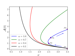
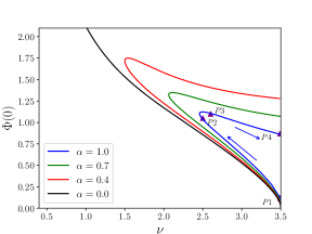
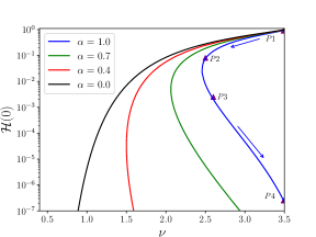
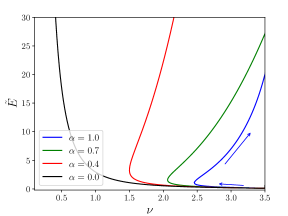
Figure 1: Values of the three fields at the Q-ball center and the total energy $\tilde{E}$ for different values of gauge coupling $\alpha$. The arrows represent the evolution of the frequency $\nu$. We choose $k=3.5$ which corresponds to $\lambda_{\phi h}\approx 6$. Four specific solutions $P1,P2,P3,P4$ for $\alpha=1.0$ are marked by the triangles and the corresponding profiles are shown in figure 2.

After qualitative analysis of the gauged Q-ball solution, we begin to numerically solve Eqs. (7), (8), and (9) with the following boundary conditions,

$$\frac{\partial\mathcal{A}}{\partial\rho}=\frac{\partial\Phi}{\partial\rho}=\frac{\partial\mathcal{H}}{\partial\rho}=0\text{ at }\rho=0,\quad\mathcal{A}=\Phi=0\text{ and }\mathcal{H}=1\text{ at }\rho=\infty\,\,.$$ (22)

The first boundary condition is necessary so that the terms $\frac{2}{\rho}\left(\frac{\partial\mathcal{A}}{\partial\rho}\right),\frac{2}{\rho}\left(\frac{\partial\Phi}{\partial\rho}\right)$, and $\frac{2}{\rho}\left(\frac{\partial\mathcal{H}}{\partial\rho}\right)$ do not become singular at $\rho=0$, and the latter is necessary because the energy density $\mathcal{E}$ and charge density $(\nu-\alpha^{2}\mathcal{A})\Phi^{2}$ should be integrable over the infinite spatial volume and the integral should be finite.

It is convenient to introduce the dimensionless quantities for the total energy and charge of the gauged Q-ball,

$$\tilde{E} \equiv\frac{\lambda_{h}}{2\pi m_{\phi}}E=\frac{1}{k}\int_{0}^{\infty}d\rho\rho^{2}\mathcal{E}\,\,,$$ (23)

$$\tilde{Q} \equiv\frac{\lambda_{h}Q}{2\pi}=\int_{0}^{\infty}d\rho\rho^{2}(\nu-\alpha^{2}\mathcal{A})\Phi^{2}\,\,,$$

which can be calculated directly once the numerical solutions of the corresponding differential equations are found.

We use the relaxation method NumericalRecipes ; Guo:2020tla to solve coupled 2nd order ordinary differential equations, Eqs. (7), (8) and (9), with boundary conditions, Eq. (22). The relaxation method solves the boundary value problems by updating the trial functions on the grid in an iterative way. As an example, we fix $k=3.5$ and we scan over all of the solutions at a given value of $\alpha$. The results can be seen from figure 1. The frequency $\nu$ firstly decreases in the direction of the arrow. We call this the “first branch” where the back reaction of gauge field is small. Then the solutions turn on the “second branch” where $\nu$ increases and the gauge field dominates. Contrary to the global Q-ball, the parameter $\nu$ does not uniquely determine the charge and energy of the gauged Q-ball. For the global case, the energy and charge increase as the $\nu$ approaches zero. However, in the case of gauged Q-ball, the $\nu$ is replaced by $\nu-\alpha^{2}\mathcal{A}$. Then on the second branch where the gauge field $\mathcal{A}$ dominates, $\nu$ has to increase in order to satisfy $\nu-\alpha^{2}\mathcal{A}>0$.

We choose four specific solutions $P1,P2,P3,P4$ in figure 1 for $\alpha=1.0$ which are marked by the purple triangles and the corresponding numerical profiles of $\mathcal{A}$, $\Phi$ and $\mathcal{H}$ are shown in figure 2. We can see that as the value of $\mathcal{A}(0)$ of the gauged Q-ball becomes larger, the Higgs field value inside the Q-ball is closer to zero. Actually, when the value of $\mathcal{A}(0)$ becomes larger, the radius, charge and energy also increase, so we can say that the Higgs value is effectively zero inside large gauged Q-balls.

The total charge of gauged Q-ball for different values of gauge coupling $\alpha$ is shown in the left panel of figure 3. It can seen that the charge for the gauged Q-ball is also finite at a nonzero $\alpha$. However, for the global Q-ball the charge is unbounded from above. In order to obtain a gauged Q-ball with relatively large charge, the gauge coupling has to be small enough.

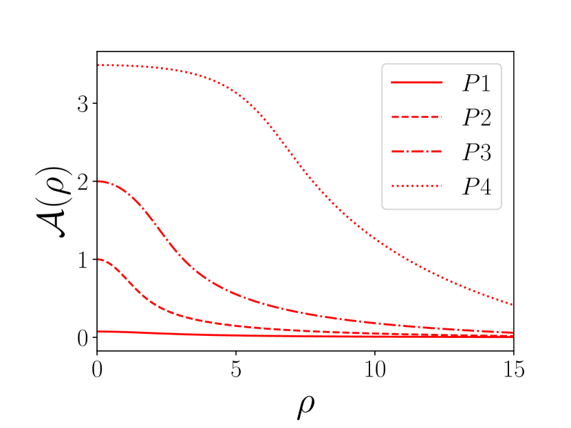
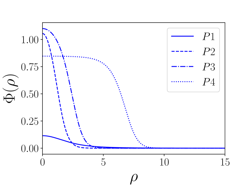
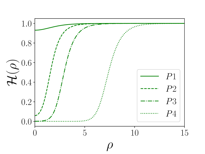
Figure 2: Profiles of the dark gauge field, complex scalar field, Higgs field of the gauged Q-ball. Here we choose the marked points $P1,P2,P3,P4$ in figure 1 where $k=3.5$ and $\alpha=1.0$.

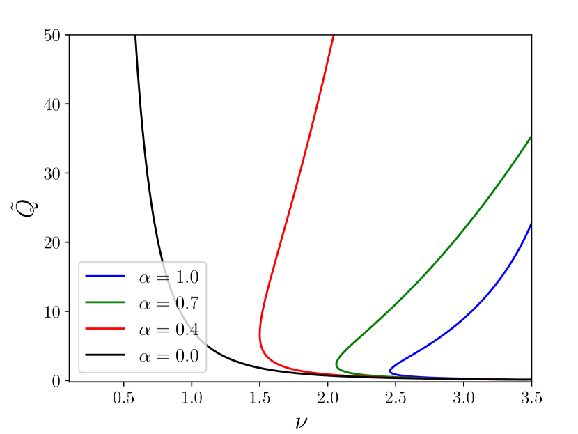
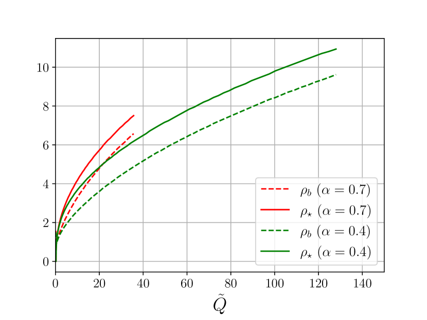
Figure 3: Left: total charge $\tilde{Q}$ for different values of $\alpha$ for $U(1)$ gauged Q-balls. Right: the two typical radius for the Q-ball field $\Phi(\rho)$ and Higgs field $\mathcal{H}(\rho)$.

We can define two typical radius for the Higgs field $\mathcal{H}(\rho)$ and the Q-ball field $\Phi(\rho)$ respectively. The $\rho_{\star}$ is defined by $\mathcal{H}(\rho_{\star})=1/2$ and $\rho_{b}$ is defined by $\Phi(\rho_{b})=\Phi(0)/2$. These two radius are shown in the right panel of figure 3. It can be seen that $\rho_{\star}$ is generally larger than $\rho_{b}$. One may prefer to call $\rho_{\star}$ the radius of the “Higgs ball”. Hereafter, we use $\rho_{\star}$ to represent the Q-ball radius which defines the charge and energy of gauged Q-balls.

3 Basic properties of gauged Q-balls

3.1 $dE/dQ$ for gauged Q-balls

It is well known that for non-gauged Q-balls the relations $dE/dQ=\omega$ holds. Here we will show that this also holds for gauged Q-balls in FLSM model. From Eq. (10), we have

$$\frac{dE}{d\nu} =\frac{4\pi v_{0}}{\sqrt{2\lambda_{h}}}\int d\rho\rho^{2}\left\{\alpha^{2}\left(\partial_{\rho}\mathcal{A}\right)\left(\partial_{\rho}\frac{d\mathcal{A}}{d\nu}\right)+\left(\partial_{\rho}\Phi\right)\left(\partial_{\rho}\frac{d\Phi}{d\nu}\right)+\left(\partial_{\rho}\mathcal{H}\right)\left(\partial_{\rho}\frac{d\mathcal{H}}{d\nu}\right)\right.$$

$$+\left[\left(1-\alpha^{2}\frac{d\mathcal{A}}{d\nu}\right)(\nu-\alpha^{2}\mathcal{A})+k^{2}\mathcal{H}\frac{d\mathcal{H}}{d\nu}\right]\Phi^{2}+\left[(\nu-\alpha^{2}\mathcal{A})^{2}+k^{2}\mathcal{H}^{2}\right]\Phi\frac{d\Phi}{d\nu}$$

$$\left.+\frac{1}{2}\left(\mathcal{H}^{2}-1\right)\mathcal{H}\frac{d\mathcal{H}}{d\nu}\right\}\,\,.$$ (24)

After integrating $\partial_{\rho}\Phi$ and $\partial_{\rho}\mathcal{H}$ by part and using Eqs. (8) and (9), we can get

$$\frac{dE}{d\nu} =\frac{4\pi v_{0}}{\sqrt{2\lambda_{h}}}\int d\rho\rho^{2}\left[\alpha^{2}\left(\partial_{\rho}\mathcal{A}\right)\left(\partial_{\rho}\frac{d\mathcal{A}}{d\nu}\right)+(\nu-\alpha^{2}\mathcal{A})\left(1-\alpha^{2}\frac{d\mathcal{A}}{d\nu}\right)\Phi^{2}+2(\nu-\alpha^{2}\mathcal{A})^{2}\Phi\frac{d\Phi}{d\nu}\right]$$ (25)

$$=\frac{4\pi v_{0}}{\sqrt{2\lambda_{h}}}\int d\rho\rho^{2}\left\{(\nu-\alpha^{2}\mathcal{A})\frac{d}{d\nu}\left[(\nu-\alpha^{2}\mathcal{A})\Phi^{2}\right]+\alpha^{2}\left(\partial_{\rho}\mathcal{A}\right)\left(\partial_{\rho}\frac{d\mathcal{A}}{d\nu}\right)\right\}$$

$$=\sqrt{2\lambda_{h}}v_{0}\nu\frac{dQ}{d\nu}+\underbrace{\frac{4\pi v_{0}}{\sqrt{2\lambda_{h}}}\int d\rho\rho^{2}\left\{-\alpha^{2}\mathcal{A}\frac{d}{d\nu}\left[(\nu-\alpha^{2}\mathcal{A})\Phi^{2}\right]+\alpha^{2}\left(\partial_{\rho}\mathcal{A}\right)\left(\partial_{\rho}\frac{d\mathcal{A}}{d\nu}\right)\right\}}_{=0}\,\,.$$

In the third line we have integrated $\partial_{\rho}\mathcal{A}$ by part and used Eq. (7), then the integral vanishes. Finally,

$$\frac{dE}{d\omega}=\frac{dE}{d\nu}\frac{d\nu}{d\omega}=\left(\sqrt{2\lambda_{h}}v_{0}\omega\frac{dQ}{d\omega}\right)\left(\frac{1}{\sqrt{2\lambda_{h}}v_{0}}\right)=\omega\frac{dQ}{d\omega}\,\,,$$ (26)

which leads to

$$\frac{dE}{dQ}=\omega$$ (27)

for $\frac{dQ}{d\omega}\neq 0$. The existence of $\frac{dQ}{d\omega}=0$ indicates the locally minimal or locally maximal charge.

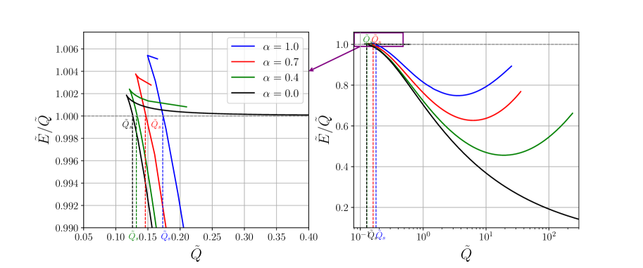
Figure 4: The energy over charge $\tilde{E}/\tilde{Q}$ for different values of $\alpha$. The $\tilde{Q}_{s}$ represents the value of charge which satisfies $\tilde{E}/\tilde{Q}=1$.

3.2 Stability of gauged Q-balls

The stability of the Q-ball is an important criterion to judge whether it can serve as the DM candidate. Unlike the global Q-balls, the stability of gauged Q-balls is still being discussed. In this subsection, we will systematically analyze four stability criteria of gauged Q-balls and show the viable parameter space of stable gauged Q-balls.

3.2.1 Quantum mechanical stability

The quantum mechanical stability is satisfied if

$$E<m_{\phi}Q\quad\text{or}\quad\tilde{E}/\tilde{Q}<1\,\,.$$ (28)

This means that the gauged Q-ball is stable against decay to free scalar particles. It should be noted that if the Q-ball has decay channels into other fundamental scalar particles which have the mass $m_{i}$ that are smaller than $m_{\phi}$, we need to replace $m_{\phi}$ by $m_{i}$ in Eq. (28). The decay of global Q-balls or gauged Q-balls has been discussed in several works Cohen:1986ct ; Kawasaki:2012gk ; Hong:2017uhi ; Kasuya:2012mh . When the effective energy of DM particles inside the gauged Q-balls $\pi/r_{\star}\propto(\omega-\tilde{g}\tilde{A}_{t})$ is larger than the masses of decay products, the decay process is kinetically allowed. In our case, the gauged Q-balls decay mainly through the process $\phi^{\dagger}\phi\rightarrow hh$. However, as the Q-ball radius $r_{\star}$ is large enough or $(\omega-\tilde{g}\tilde{A}_{t})$ is small, the gauged Q-balls are stable against decaying into 125 GeV Higgs particles.

The ratio $\tilde{E}/\tilde{Q}$ is shown in the figure 4. As the frequency $\nu\rightarrow k$ on the first branch, there is a region of parameter space where $\tilde{E}/\tilde{Q}>1$. It implies the existence of a minimal Q-ball charge $\tilde{Q}_{s}$ defined as $\tilde{E}(Q_{s})/\tilde{Q}_{s}=1$ of the quantum mechanically stable gauged Q-ball. We can see from figure 4 that for the global Q-balls the $\tilde{E}/\tilde{Q}$ decreases with growing $\tilde{Q}$ when $\tilde{E}/\tilde{Q}<1$. The branch of $\tilde{E}/\tilde{Q}>1$ corresponds to $\nu\rightarrow k$. So the global Q-balls are quantum mechanically stable as $\nu\ll k$ and $\tilde{Q}>\tilde{Q}_{s}$. One would wonder that the gauged Q-ball will destroy the quantum mechanical stability at large charge because the dark electrostatic energy is proportional to $\tilde{Q}^{2}$ and thus the $\tilde{E}/\tilde{Q}$ is proportional to $\tilde{Q}$. However, we found the gauged Q-balls is always quantum mechanically stable on the second branch where the gauge field dominates because of the charge of the gauged Q-balls must be finite.

3.2.2 Stress stability

Now we investigate the effect of the electrostatic repulsion on the stability of the gauged Q-balls. In Ref. Loiko:2022noq , the authors pointed out that, just like the hadrons, a necessary condition for stability of the configuration of gauged Q-balls is the balance of the internal forces, called von Laue condition Laue:1911lrk ; Bialynicki-Birula:1993shm

$$\int_{0}^{\infty}drr^{2}p(r)=0\,\,.$$ (29)

Here $p(r)$ is the radial distribution of the pressure inside the Q-ball, which can be extracted from the energy-momentum tensor by using the following parametrization Polyakov:2002yz ; Mai:2012yc :

$$T_{ij}=\left(\hat{r}_{i}\hat{r}_{j}-\frac{1}{3}\delta_{ij}\right)s(r)+\delta_{ij}p(r)\,\,.$$ (30)

$s(r)$ is the traceless part which yields the anisotropy of pressure (shear forces). This kind of stability has also been studied on global Q-balls Mai:2012yc ; Polyakov:2018zvc .

One stronger local constraint is that the normal force per unit area acting on an infinitesimal area element at a distance $r$, must be directed outward Perevalova:2016dln ; Polyakov:2018zvc ,

$$F(r)=\frac{2}{3}s(r)+p(r)>0\,\,.$$ (31)

This is a necessary but not sufficient condition for stability. By using the rescaled parameters, we have the expressions of $p(\rho)$ and $s(\rho)$ in the FLSM model:

$$p(\rho) =2\lambda_{h}v_{0}^{4}\left[-\frac{1}{6}(\partial_{\rho}\Phi)^{2}-\frac{1}{6}(\partial_{\rho}\mathcal{H})^{2}+\frac{\alpha^{2}}{6}(\partial_{\rho}\mathcal{A})^{2}+\frac{1}{2}(\nu-\alpha^{2}\mathcal{A})^{2}\Phi^{2}-\frac{k^{2}}{2}\Phi^{2}\mathcal{H}^{2}-\frac{1}{8}(\mathcal{H}^{2}-1)^{2}\right]\,\,,$$ (32)

$$s(\rho) =2\lambda_{h}v_{0}^{4}\left[(\partial_{\rho}\Phi)^{2}+(\partial_{\rho}\mathcal{H})^{2}-\alpha^{2}(\partial_{\rho}\mathcal{A})^{2}\right]\,\,,$$

from which we get

$$F(\rho)=2\lambda_{h}v_{0}^{4}\left[\frac{1}{2}(\partial_{\rho}\Phi)^{2}+\frac{1}{2}(\partial_{\rho}\mathcal{H})^{2}-\frac{\alpha^{2}}{2}(\partial_{\rho}\mathcal{A})^{2}+\frac{1}{2}(\nu-\alpha^{2}\mathcal{A})^{2}\Phi^{2}-\frac{k^{2}}{2}\Phi^{2}\mathcal{H}^{2}-\frac{1}{8}(\mathcal{H}^{2}-1)^{2}\right]\,\,.$$ (33)

In figure 5, we show the profile of $F(\rho)$ for four marked points in figure 1. We can see that the $F(\rho)$ has no nodes for $P1$ and $P2$ on the first branch. $F(\rho)$ has negative values on the second branch so the gauged Q-balls on the second branch where gauge potential dominates are unstable. It should be noted that the inequality (31) takes a approximation that Q-balls behave as a continuous media , which needs more discussions.

The stress-stability is the most stringent stability criterion in this work. We are not sure if the gauged Q-ball on the second branch would decay into free particles or smaller Q-balls. And it is meaningful to explore that how we can get rid of the strong constraints from stress-stability, in other words, how to get large gauged Q-balls with large gauge coupling. Maybe we can consider an example where two scalar case where the two scalars $\phi$ and $\psi$ possess opposite charges. If the electrostatic field produced by the two scalars cancels with each other, which implies

$$\tilde{g}Q_{\phi}+\tilde{g}^{\prime}Q_{\psi}=0\,\,,$$ (34)

where $\tilde{g}$ and $\tilde{g}^{\prime}$ are the gauge couplings of $\phi$ and $\psi$ respectively, this guarantees the electric neutrality of the interior of the gauged Q-balls Anagnostopoulos:2001dh ; Ishihara:2018rxg . The gauged Q-balls will avoid the electric repulsion which leads to the stress-instability even the gauge coupling is large. We expect these Q-balls can also be the DM candidate because they will behave as the ordinary global Q-balls.

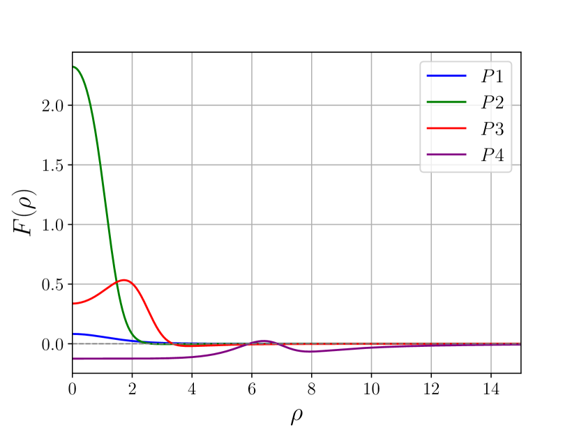
Figure 5: Profile of $F(\rho)$ defined by Eq. (33) for the four marked points in figure 1.

3.2.3 Stability against fission

For global (i.e., nongauged) Q-balls the corresponding stability criterion against fission takes the form

$$d^{2}E/dQ^{2}<0\,\,.$$ (35)

This clearly leads to $E(Q_{1})+E(Q_{2})>E(Q_{1}+Q_{2})$ when $E(0)=0$. However, this may not hold everywhere for the gauged Q-balls due to the presence of the gauge potential. In Ref. Gulamov:2013cra the authors gave a detailed discussion on the stability against fission of $U(1)$ gauged Q-balls. They pointed out that we could not make any conclusion about the stability against fission for gauged Q-balls on the second branch. Nevertheless, it has been shown that the gauged Q-balls on the first branch are generally stable because the back-reaction of the gauge field is generally small.

3.2.4 Classical stability

The problem of classical stability of $U(1)$ gauged Q-balls is discussed in detail in Ref. Panin:2016ooo . The classical stability criterion was firstly derived in Lee:1991ax for one-field Q-balls and was discussed for the model with two scalar fields in Friedberg:1976me . The proof of Refs. Friedberg:1976me ; Lee:1991ax was based on examining the properties of the energy functional of the system. Instead, the examination of Ref. Panin:2016ooo is based on the Vakhitov-Kolokolov method 1973Stationary ; 1978Dynamics which utilized linearized EoM for the perturbations above the background solution.

We only consider the spherical perturbations on the gauged Q-ball. We adopt the following ansatz:

$$\phi(t,r) =e^{-i\omega t}f(r)+e^{-i\omega t}e^{\gamma t}(u(r)+il(r))\,\,,$$ (36)

$$\tilde{A}_{t}(t,r) =\tilde{A}_{t}(r)+e^{\gamma t}a_{0}(r)\,\,,$$

$$h(t,r) =h(r)+e^{\gamma t}\sigma(r)\,\,,$$

where $f(r)$, $\tilde{A}_{t}(r)$ and $h(r)$ are the background solutions. $u(r)$, $l(r)$, $a_{0}(r)$ and $\sigma(r)$ are the perturbations on the background. Then we obtain the linearized EoM as below,

$$\Delta u+(\omega-\tilde{g}\tilde{A}_{t})^{2}u-\gamma^{2}u-2(\omega-\tilde{g}\tilde{A}_{t})\gamma l-2\tilde{g}(\omega-\tilde{g}\tilde{A}_{t})fa_{0}-Uu-2Su-Y\sigma=0\,\,,$$ (37)

$$\Delta l+(\omega-\tilde{g}\tilde{A}_{t})^{2}l-\gamma^{2}l+2(\omega-\tilde{g}\tilde{A}_{t})\gamma u-\tilde{g}\gamma fa_{0}-Ul=0\,\,,$$

$$\Delta a_{0}-2\tilde{g}^{2}f^{2}a_{0}+4\tilde{g}(\omega-\tilde{g}\tilde{A}_{t})fu-2\tilde{g}\gamma fl=0\,\,,$$

$$\Delta\sigma-\gamma^{2}\sigma-W\sigma-2Yu=0\,\,.$$

where $\Delta=\sum_{i=1}^{3}\partial_{i}\partial_{i}$ is the 3-dim Laplacian operator and

$$U(r)=\left.\frac{\partial V}{\partial(\phi^{*}\phi)}\right|_{\begin{subarray}{c}\phi^{*}\phi=f^{2}(r)\\ h=h(r)\end{subarray}},\quad S(r)=\left.\frac{\partial^{2}V}{\partial(\phi^{*}\phi)^{2}}\right|_{\begin{subarray}{c}\phi^{*}\phi=f^{2}(r)\\ h=h(r)\end{subarray}}f^{2}(r)\,\,,$$ (38)

$$W(r)=\left.\frac{1}{2}\frac{\partial^{2}V}{\partial h^{2}}\right|_{\begin{subarray}{c}\phi^{*}\phi=f^{2}(r)\\ h=h(r)\end{subarray}},\quad Y(r)=\left.\frac{\partial^{2}V}{\partial\left(\phi^{*}\phi\right)\partial h}\right|_{\begin{subarray}{c}\phi^{*}\phi=f^{2}(r)\\ h=h(r)\end{subarray}}f(r)\,\,.$$

The boundary conditions are

$$u^{\prime}(0)=l^{\prime}(0)=a_{0}^{\prime}(0)=\sigma^{\prime}(0)=0,\quad u(\infty)=l(\infty)=a_{0}(\infty)=\sigma(\infty)=0\,\,.$$ (39)

We want to obtain the parameter $\gamma$ of perturbations $u,l,a_{0},\sigma$. The classically unstable mode correspond to $\gamma>0$. We can do this by using the shooting method in Ref. Levkov:2017paj . We introduce four basis solutions $\Psi^{(i=1,2,3,4)}(r)=(u^{(i)},l^{(i)},a_{0}^{(i)},\sigma^{(i)})$ which satisfy the Neumann boundary conditions $d\Psi^{(i)}/dr|_{r=0}=0$ and Dirichlet boundary conditions $\Psi^{(1)}(0)=(1,0,0,0)$, $\Psi^{(2)}(0)=(0,1,0,0)$, $\Psi^{(3)}(0)=(0,0,1,0)$ and $\Psi^{(4)}(0)=(0,0,0,1)$. Then we integrate the Eqs. (37) numerically to find the values of $\Psi^{(i)}$ at large $r=r_{\infty}$. Now, recall that we are searching for a specific solution $\Psi(r)=c_{1}\Psi^{(1)}(r)+c_{2}\Psi^{(2)}(r)+c_{3}\Psi^{(3)}(r)+c_{4}\Psi^{(4)}(r)$ which satisfies $\Psi(r_{\infty})=0$. This gives the system of linear equations,

$$\hat{D}_{c}(c_{1},c_{2},c_{3},c_{4})^{T}=0,\quad\hat{D}_{c}=(\Psi^{(1)T},\Psi^{(2)T},\Psi^{(3)T},\Psi^{(4)T})\,\,.$$ (40)

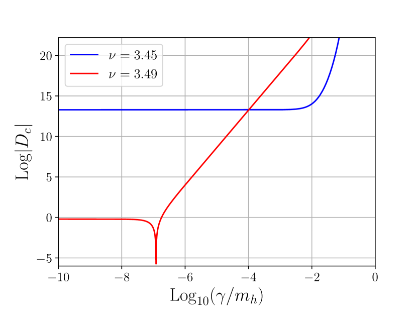
Figure 6: Determinant of matrix for $\nu=3.45$ and $\nu=3.49$ on the first branch respectively. We choose $\alpha^{2}=10^{-5}$, $k=3.5$.

Equation (40) has nontrivial solutions only if $D_{c}\equiv\det\hat{D}_{c}=0$. In figure 6 we plot $\mathrm{Log}|D_{c}|$ as a function of $\mathrm{Log}_{10}\gamma$ where we choose $\alpha^{2}=10^{-5}$ and $k=3.5$. We found that there is no classically unstable mode for $\nu=3.45$ as there is no solution for $\gamma>0$. This also hold for other solutions of $U(1)$ gauged Q-balls except for $\nu\rightarrow k$ on the first branch. We found there is one unstable mode for $\nu=3.49$. Actually, in the limit $\nu\rightarrow k$, the contribution of gauged field can be neglected and one expects that the case is similar to the non-gauged Q-ball where $\frac{dQ}{d\omega}>0$ indicates there exists classically unstable mode. This is also discussed in Refs. Friedberg:1976me ; Panin:2016ooo . However, we usually do not have to worry about this because the region already has been excluded by the quantum instability. In Ref. Kinach:2022jdx , the authors have shown that the gauged Q-balls on the second branch with small gauge coupling are classically unstable with respect to axisymmetric perturbations. This enhances our confidence that the gauged Q-ball on the second branch is unstable. The region is almost covered by the stress stability criterion.

In summary, the parameter space of gauged Q-balls are shown in figure 7. The red line represents the region where the gauged Q-ball is dominated by the gauge field such that it is unstable under stress stability criterion. The green line represents the region where the gauged Q-ball is unstable under quantum stability criterion. We only plot the quantum mechanical stability and the stress stability criterion because they cover the space which is classically unstable and is unstable against fission respectively. The gauged Q-ball is stable only in the region of $\nu\in[\nu_{\mathrm{min}},\nu_{\mathrm{max}}]$. The $\nu_{\mathrm{min}}$ corresponds to the maximal charge of gauged Q-balls. In order to form a gauged Q-ball of given charge at given gauge coupling, the charge has to be smaller than the maximal charge. It should also be noted that, if the dark gauge boson of gauged Q-ball kinetically mixes with SM photons or $Z$ bosons, this would produce distinct experimental signatures which can constrain Q-ball charge and couplings.

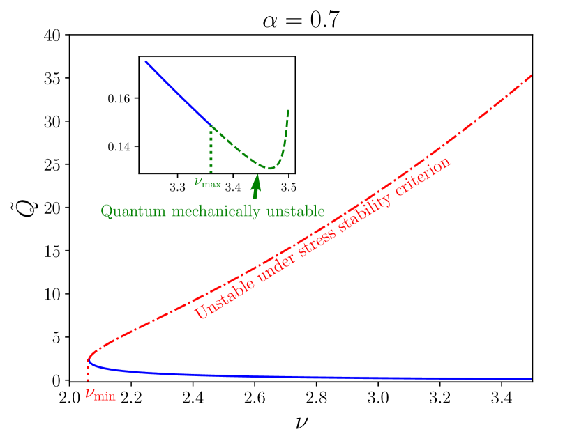
Figure 7: Viable space of $\nu$ of gauged Q-balls for $\alpha=0.7$. The red line represents the region where the gauged Q-ball is dominated by gauge field such that it is unstable under stress stability criterion. The green line represents the region where the gauged Q-ball is unstable under quantum stability criterion. Gauged Q-balls in the blue region between $\nu_{\mathrm{min}}$ and $\nu_{\mathrm{max}}$ are stable.

4 Thin-wall approximation

As the radius of gauged Q-ball becomes large, the width of profile can be neglected and the gauged Q-balls can be depicted by the thin-wall approximation. The Higgs profile can be approximately viewed as a step function, the vacuum value is zero and $v_{0}$ inside and outside the Q-ball, respectively. The derivative of the Higgs field only contributes to the surface term of gauged Q-ball which is negligible when the radius of the ball is large. Then the problems are reduced to those or ones with two fields, $\phi$ and $\tilde{A}_{\mu}$. We will discuss the simplified piecewise model and show that it behaves closely to the FLSM model. By using the mapping method introduced by Ref. Heeck:2021zvk , we give some semi-analytic results and some analytic evaluations of the maximal charge of gauged Q-balls.

4.1 Piecewise model

If the Higgs field is approximately $h(\rho)=v_{0}\Theta(\rho-\rho_{\star})$, then we can approximately view the complex scalar moving in the piecewise parabolic potential Rosen:1968mfz ; Gulamov:2013ema ; Kim:2023zvf . The Lagrangian density can be further approximated as

$$\mathcal{L}_{\mathrm{piecewise}}=\left(D_{\mu}\phi\right)^{\dagger}\left(D^{\mu}\phi\right)-\frac{1}{4}\tilde{A}_{\mu\nu}\tilde{A}^{\mu\nu}-m_{\phi}^{2}\phi^{\dagger}\phi\Theta\left(1-\frac{\phi^{\dagger}\phi}{v^{2}}\right)-m_{\phi}^{2}v^{2}\Theta\left(\frac{\phi^{\dagger}\phi}{v^{2}}-1\right)\,\,,$$ (41)

where $\Theta(x)$ is the Heaviside step function. In our case,

$$m_{\phi}=v_{0}\sqrt{\frac{\lambda_{\phi h}}{2}},\quad v=v_{0}\sqrt{\frac{\lambda_{h}}{2\lambda_{\phi h}}}\,\,.$$ (42)

Note that $v$ is chosen so that $V(\phi)$ is continuous at $\phi^{\dagger}\phi=v^{2}$. This can be understood from the EoM of the Higgs field in the FLSM model,

$$h^{\prime\prime}(r)+\frac{2}{r}h^{\prime}(r)+\left[\frac{m_{h}^{2}}{2}-\lambda_{h}h(r)^{2}-\lambda_{\phi h}f(r)^{2}\right]h(r)=0\,\,,$$ (43)

where we use the definition $\phi(r,t)=f(r)e^{-i\omega t}$ and the prime denotes a derivative with respect to $r$. If the Higgs field is approximately a step function, we can neglect the derivatives, then we have

$$h^{2}\approx\begin{cases}\frac{m_{h}^{2}}{2\lambda_{h}}-\frac{\lambda_{\phi h}}{\lambda_{h}}f^{2}\quad\text{for}\quad 2\lambda_{\phi h}f^{2}<m_{h}^{2}\,\,,\\ 0\quad\text{for}\quad 2\lambda_{\phi h}f^{2}>m_{h}^{2}\,\,,\end{cases}$$ (44)

and we could assume $f(r)\approx 0$ outside the bubble, for which $h^{2}\approx\frac{m_{h}^{2}}{2\lambda_{h}}=v_{0}^{2}$. Therefore $V(\phi,h)\approx m_{\phi}^{2}\phi^{\dagger}\phi$ outside the Q-ball and $V(\phi,h)\approx\frac{\lambda_{h}}{4}v_{0}^{4}$ inside the Q-ball. The consistency between the piecewise model and the Friedberg-Lee-Sirlin model has been discussed in Ref. Kim:2023zvf and the classical stability of gauged Q-balls in piecewise model has been studied in Ref. Panin:2016ooo ; Gulamov:2013ema . The EoM of gauged Q-balls in the piecewise model after the rescaling of Eq. (19) are

$$\frac{1}{\rho^{2}}\partial_{\rho}\left(\rho^{2}\partial_{\rho}\mathcal{A}\right)+(\nu-\alpha^{2}\mathcal{A})\Phi^{2}=0\,\,,$$ (45)

$$\frac{1}{\rho^{2}}\partial_{\rho}\left(\rho^{2}\partial_{\rho}\Phi\right)+\left[(\nu-\alpha^{2}\mathcal{A})^{2}-k^{2}\Theta\left(1-4k^{2}\Phi^{2}\right)\right]\Phi=0\,\,.$$ (46)

These equations are easier to solve than the FLSM model by using undershooting/overshooting method. The Q-ball energy and charge reads,

$$\tilde{E}=\frac{1}{k}\int_{0}^{\infty}d\rho\rho^{2}\mathcal{E},\quad\tilde{Q}=\int_{0}^{\infty}d\rho\rho^{2}(\nu-\alpha^{2}\mathcal{A})\Phi^{2}\,\,.$$ (47)

Here, $\mathcal{E}=\frac{\alpha^{2}}{2}\left(\partial_{\rho}\mathcal{A}\right)^{2}+\frac{1}{2}\left(\partial_{\rho}\Phi\right)^{2}+\frac{1}{2}\left[(\nu-\alpha^{2}\mathcal{A})^{2}+k^{2}\Theta(1-4k^{2}\Phi^{2})\right]\Phi^{2}+\frac{1}{8}\Theta(4k^{2}\Phi^{2}-1)$ which has a different form form the FLSM model.

We solve Eqs. (45) and (46) numerically to get the profiles of the complex field and the gauge field. Then we can get the charge and energy of gauged Q-balls by substituting them into Eqs. (47). These numerical results are shown in figure 8. We can see that the piecewise model fits the FLSM model well when the gauged Q-ball radius is large. The distinctions appear at small $\rho_{\star}$ at which the Higgs field value inside is not approximately zero.

4.2 Mapping gauged Q-balls

We make a further assumption that the complex scalar field is also a step function, $\Phi(\rho)=\Phi_{0}(1-\Theta(\rho-\rho_{b}))$, where we denote $\Phi_{0}=\Phi(0)$ and $\rho_{b}$ is defined by $\Phi(\rho_{b})=\Phi_{0}/2$. Then the profile of gauged field is Lee:1988ag

$$\mathcal{A}(\rho)=\frac{\nu}{\alpha^{2}}\begin{cases}1-\frac{\sinh(\alpha\Phi_{0}\rho)}{\cosh(\alpha\Phi_{0}\rho_{b})\alpha\Phi_{0}\rho},&\rho<\rho_{b}\\ \frac{\alpha\Phi_{0}\rho_{b}-\tanh(\alpha\Phi_{0}\rho_{b})}{\alpha\Phi_{0}\rho},&\rho>\rho_{b}\,\,.\end{cases}$$ (48)

The Q-ball radius is defined by $\Phi(\rho_{\star})=\frac{1}{2k}$.

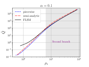
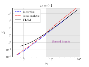
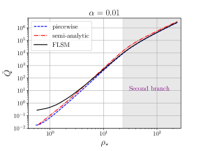
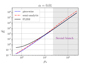
Figure 8: Charge and Energy as functions of Gauged Q-ball radius. The blue lines are the numerical results in piecewise model; red lines are the semi-analytic results Eq. (52) and Eq. (55), black lines come from the numerical results in FLSM model.

In Ref. Heeck:2021zvk , the authors propose a mapping between the gauged Q-ball and the global Q-ball. Specifically,

$$\nu=\nu_{g}\alpha\Phi_{0}\rho_{b}\coth(\alpha\Phi_{0}\rho_{b})\,\,,$$ (49)

where $\nu_{g}$ is the value of frequency for the global Q-ball with the same $\rho_{b}$. Then the profile of $\mathcal{A}$ is given by Eq. (48). This relation holds even for cases beyond the thin-wall approximation. Interestingly, the global cases in the piecewise model have analytic solutions Gulamov:2013ema :

$$\Phi_{g}(\rho)=\begin{cases}\frac{1}{2k}\frac{\rho_{\star}\sin(\nu_{g}\rho)}{\rho\sin(\nu_{g}\rho_{\star})},&\rho<\rho_{\star}\\ \frac{1}{2k}\frac{\rho_{\star}e^{-\sqrt{k^{2}-\nu_{g}^{2}}\rho}}{\rho e^{-\sqrt{k^{2}-\nu_{g}^{2}}\rho_{\star}}},&\rho>\rho_{\star}\,\,.\end{cases}$$ (50)

This gives us $\Phi_{0}=\frac{1}{2k}\frac{\nu_{g}\rho_{\star}}{\sin(\nu_{g}\rho_{\star})}$ and $2\sin(\nu_{g}\rho_{b})=\nu_{g}\rho_{b}$. Then we have $\nu_{g}\rho_{b}=C_{1}$ where $C_{1}\approx 1.89549$. The Q-ball radius is defined as

$$\rho_{\star}(\nu_{g})=\frac{1}{\nu_{g}}\left(\pi-\arctan\left(\frac{\nu_{g}}{\sqrt{k^{2}-\nu_{g}^{2}}}\right)\right)\,\,.$$ (51)

If we use $\Phi(\rho)=\Phi_{0}(1-\Theta(\rho-\rho_{b}))$ and $\mathcal{A}(\rho)$ from Eq. (48), we have further semi-analytic results for charge:

$$\tilde{Q}=\frac{\nu_{g}\rho_{b}}{\alpha^{2}}\left(\alpha\Phi_{0}\rho_{b}\coth(\alpha\Phi_{0}\rho_{b})-1\right)=\frac{\rho_{b}}{\alpha^{2}}(\nu-\nu_{g})\,\,.$$ (52)

In the limit $\alpha\rightarrow 0$ and $\alpha\Phi_{0}\rho_{b}\rightarrow 0$, because $x\coth x\sim 1+\frac{x^{2}}{3}+\mathcal{O}(x^{3})$ for $x\rightarrow 0$. Then we have $\tilde{Q}\sim\nu_{g}\Phi_{0}^{2}\rho_{b}^{3}$. And in this case, when $\nu_{g}\rightarrow 0$, from Eq. (51) we have $\nu_{g}\rho_{\star}\simeq\pi$ and $\sin(\nu_{g}\rho_{\star})\simeq\nu_{g}/k$, which lead to

$$\Phi_{0}\simeq\frac{1}{2k}\frac{\pi}{\nu_{g}/k}=\frac{\pi}{2\nu_{g}}\,\,.$$ (53)

From $2\sin(\nu_{g}\rho_{b})=\nu_{g}\rho_{b}$, we have $\nu_{g}\sim\frac{C_{1}}{\rho_{b}}$, and

$$\tilde{Q}\propto\rho_{b}^{4}\,\,,$$ (54)

which is consistent with the global Q-ball case. Using the same procedure that derives Eq. (2.1), we have analytic results for total energy:

$$\tilde{E} =\frac{\nu\tilde{Q}}{k}+\frac{1}{3k}\int d\rho\rho^{2}\left[\left(\partial_{\rho}\Phi\right)^{2}-{\alpha^{2}}\left(\partial_{\rho}\mathcal{A}\right)^{2}\right]$$ (55)

$$\simeq\frac{\nu\tilde{Q}}{k}+\frac{\Phi_{0}\rho_{b}^{2}}{12k}-\frac{1}{3k}\frac{\nu^{2}\left[\alpha\Phi_{0}\rho_{b}(2+\mathrm{sech}^{2}(\alpha\Phi_{0}\rho_{b}))-3\tanh(\alpha\Phi_{0}\rho_{b})\right]}{2\alpha^{3}\Phi_{0}}\,\,.$$

The second term comes from the integration over discontinuous $(\partial_{\rho}\Phi)^{2}$ by using the approximation of energy conservation Heeck:2020bau .

In the first limit of $\alpha\Phi_{0}\rho_{b}\rightarrow 0$ and large $\rho_{b}$, the last term of Eq. (55) vanishes. We have $\nu\simeq\nu_{g}$, $\Phi_{0}\simeq\frac{\pi}{2\nu_{g}}\simeq\frac{\rho_{\star}}{2}$ and $\rho_{\star}\simeq\rho_{b}$, then

$$\tilde{E}\simeq\frac{\pi\tilde{Q}}{k\rho_{b}}+\frac{\rho_{b}^{3}}{24k}\,\,,$$ (56)

which is just the energy of global Q-ball.

In the opposite limit $\alpha\Phi_{0}\rho_{b}\rightarrow\infty$, because $\mathcal{A}\rightarrow\tilde{Q}/\rho$, then from Eq. (48),

$$\nu=\frac{\alpha^{2}\tilde{Q}}{\rho_{b}}\left(1-\frac{\tanh(\alpha\Phi_{0}\rho_{b})}{\alpha\Phi_{0}\rho_{b}}\right)^{-1}\simeq\frac{\alpha^{2}\tilde{Q}}{\rho_{b}}\,\,.$$ (57)

Thus from Eq. (55) the energy of gauged Q-ball is

$$\tilde{E}\simeq\frac{\nu\tilde{Q}}{k}+\frac{\Phi_{0}\rho_{b}^{2}}{12k}-\frac{1}{3k}\frac{\nu^{2}\rho_{b}}{\alpha^{2}}\simeq\frac{2\alpha^{2}\tilde{Q}^{2}}{3k\rho_{b}}+\frac{\Phi_{0}\rho_{b}^{2}}{12k}\,\,.$$ (58)

The first term is the Coulomb energy and the second term is the potential energy difference between inside and outside of the Q-ball. The second term is proportional to $\rho_{b}^{2}$ because in this case the Compton wavelength of the gauge field $\frac{1}{\tilde{g}v_{0}\Phi_{0}}$ inside the Q-ball is much smaller than Q-ball radius, $r_{b}=\rho_{b}/m_{h}$. So the Q ball is superconducting. The potential energy is therefore zero inside as well as outside of the Q ball and is nonzero only in the shell around $\rho_{b}$ Lee:1988ag .

For a given $\rho_{\star}$, we can solve the Eq. (51) to get the corresponding $\nu_{g}$. After using $\Phi_{0}=\frac{1}{2k}\frac{\nu_{g}\rho_{\star}}{\sin(\nu_{g}\rho_{\star})}$, $2\sin(\nu_{g}\rho_{b})=\nu_{g}\rho_{b}$ and Eq. (49) we can get $\Phi_{0}$, $\rho_{b}$ and $\nu$ of gauged Q-balls. Substitute them into Eqs. (52) and (55) to get the charge and energy of gauged Q-balls. These semi-analytic results are shown by the red lines in figure 8. We find the mapping works well for $\rho_{\star}\gg 1$ on the first branch where the profiles of scalar fields $\phi$ and $h$ can be safely viewed as step function. The semi-analytic results of energy doesn’t work well for the second branch because the $\Phi_{0}\neq\frac{1}{2k}\frac{\nu_{g}\rho_{\star}}{\sin(\nu_{g}\rho_{\star})}$ which is the value in the global case. The value of $\Phi_{0}$ is lower because the gauge potential dominates. This can be seen from figure 1. At the turning point between first branch and second branch, the discrepancy between semi-analytic results and numerical results is about a factor of $\mathcal{O}(1)$.

4.3 Maximal charge and energy of gauged Q-balls: analytic approximations

We give analytic evaluations of maximal charge and maximal energy of gauged Q-balls for a given gauge coupling. Because the gauged Q-balls should be unstable under stress stability criterion on the second branch where the gauge potential dominates, the maximal charge is approximately defined by $\left.\frac{d\nu}{d\rho_{\star}}\right|_{\rho_{\star}=\rho_{\mathrm{max}}}=0$. In the limit at large Q-ball with $\nu_{g}\rightarrow 0$, we have $\rho_{b}=C_{1}/\nu_{g}$ and $\Phi_{0}\simeq\frac{\rho_{\star}}{2}$. Then, from (49) we get

$$\nu=\frac{C_{1}\alpha\rho_{\star}}{2}\coth\left(\frac{C_{1}\alpha\rho_{\star}}{2\nu_{g}}\right)=\frac{C_{1}\alpha\rho_{\star}}{2}\coth\left(\frac{C_{1}\alpha\rho_{\star}^{2}}{2\pi}\right)\,\,,$$ (59)

where we used $\rho_{\star}\simeq\pi/\nu_{g}$ when $\nu_{g}\rightarrow 0$. Then we have when the charge is maximal $\left.\frac{d\nu}{d\rho_{\star}}\right|_{\rho_{\star}=\rho_{\mathrm{max}}}=0$,

$$\sinh\left(\frac{C_{1}\alpha\rho_{\mathrm{max}}^{2}}{2\pi}\right)\cosh\left(\frac{C_{1}\alpha\rho_{\mathrm{max}}^{2}}{2\pi}\right)=\frac{C_{1}\alpha\rho_{\mathrm{max}}^{2}}{\pi}\,\,,$$ (60)

then we get $\frac{C_{1}\alpha\rho_{\mathrm{max}}^{2}}{2\pi}=C_{2}$ with $C_{2}\approx 1.08866$. So in this case $\alpha\Phi_{0}\rho_{b}\simeq C_{2}$ which is somewhere in the middle of Eq. (56) and Eq. (58). We can also get the minimal frequency

$$\nu_{\mathrm{min}}=\frac{C_{1}\alpha\rho_{\mathrm{max}}}{2}\coth\left(\frac{C_{1}\alpha\rho_{\mathrm{max}}^{2}}{2\pi}\right)=\sqrt{\frac{\pi C_{1}C_{2}\alpha}{2}}\coth(C_{2})\approx 2.26\sqrt{\alpha}\,\,,$$ (61)

and the corresponding frequency for the global case $\nu_{g\mathrm{min}}=\frac{\pi}{\rho_{\mathrm{max}}}=\sqrt{\frac{\pi C_{1}\alpha}{2C_{2}}}$. We can see that $\frac{\nu_{\mathrm{min}}}{\nu_{g\mathrm{min}}}=C_{2}\coth(C_{2})\approx 1.367$ which is independent of the Q-ball size. This implies that as the solutions on the second branch are unstable, the gauged Q-ball lives on the first branch and is close to the global case.

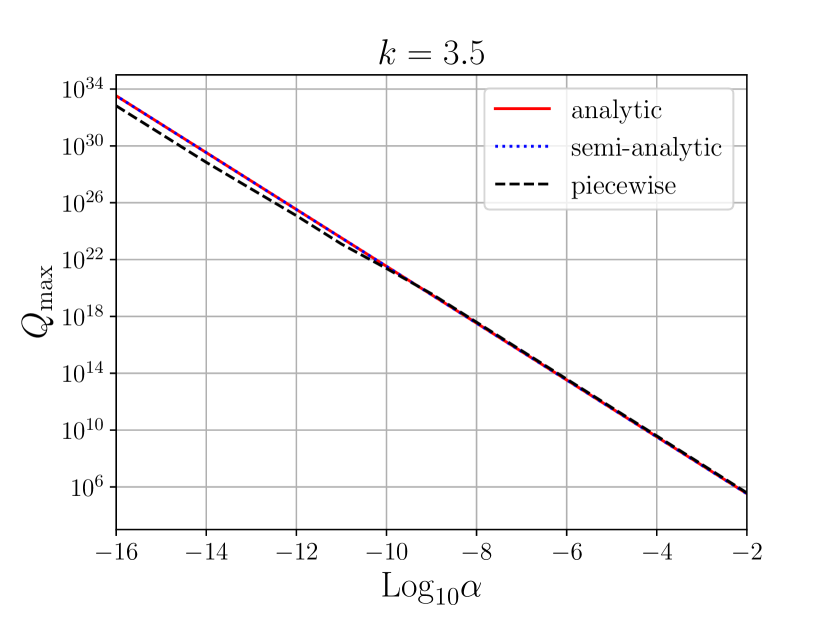
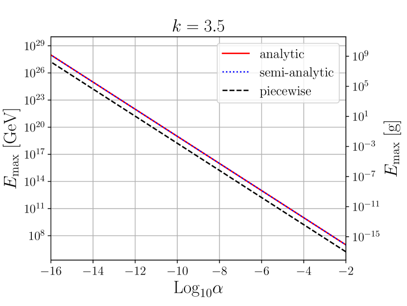
Figure 9: Maximal charge $Q_{\mathrm{max}}=\frac{2\pi}{\lambda_{h}}\tilde{Q}_{\mathrm{max}}$ (left panel) and energy $E_{\mathrm{max}}=\frac{2\pi m_{\phi}}{\lambda_{h}}\tilde{E}_{\mathrm{max}}$ (right panel) of gauged Q-ball for different $\alpha$ and $k$. The red lines are analytic evaluations Eq. (62) and (64); the blue dotted lines are the semi-analytic results and the black dashed lines represent the numerical results for piecewise model.

Finally, we get the maximal charge,

$$\tilde{Q}_{\mathrm{max}}=\frac{C_{1}}{\alpha^{2}}(C_{2}\coth C_{2}-1)\approx 0.7\alpha^{-2}\,\,,$$ (62)

from which we can see the charge is unbounded from above in the global case where $\alpha=0$. The maximal energy reads

$$\tilde{E}_{\mathrm{max}} =\frac{\nu_{\mathrm{min}}\tilde{Q}_{\mathrm{max}}}{k}+\frac{C_{1}^{2}\rho_{\mathrm{max}}^{3}}{24\pi^{2}k}-\frac{1}{3k}\frac{\nu_{\mathrm{min}}^{2}[C_{2}(2+\mathrm{sech}^{2}C_{2})-3\tanh C_{2}]}{\alpha^{3}\rho_{\mathrm{max}}}$$ (63)

$$=\frac{\pi C_{2}\coth C_{2}\tilde{Q}_{\mathrm{max}}}{k\rho_{\mathrm{max}}}+\frac{C_{1}^{2}\rho_{\mathrm{max}}^{3}}{24\pi^{2}k}-\frac{1}{3k}\frac{\pi C_{1}C_{2}\coth^{2}C_{2}[C_{2}(2+\mathrm{sech}^{2}C_{2})-3\tanh C_{2}]}{2\alpha^{2}\rho_{\mathrm{max}}}\,\,.$$

By using $\nu_{\mathrm{min}}=\sqrt{\frac{\pi C_{1}C_{2}\alpha}{2}}\coth C_{2}$ and $\rho_{\mathrm{max}}=\sqrt{\frac{2\pi C_{2}}{C_{1}\alpha}}$, we have

$$\tilde{E}_{\mathrm{max}} =\frac{1}{k\alpha^{3/2}}\sqrt{\frac{\pi C_{1}C_{2}}{72}}\left[-3C_{1}\coth C_{2}+C_{2}\left(\frac{1}{\pi}+4C_{1}+3C_{1}\mathrm{csch}^{2}C_{2}\right)\right]$$ (64)

$$\approx 1.51k^{-1}\alpha^{-3/2}\,\,.$$

This also gives us $\tilde{E}_{\mathrm{max}}\propto\rho_{\mathrm{max}}^{3}\propto\tilde{Q}_{\mathrm{max}}^{3/4}$ which is expected in the global case.

The analytic results of $Q_{\mathrm{max}}=\frac{2\pi}{\lambda_{h}}\tilde{Q}_{\mathrm{max}}$ and $E_{\mathrm{max}}=\frac{2\pi m_{\phi}}{\lambda_{h}}\tilde{E}_{\mathrm{max}}$ are shown in terms of the red lines in figure 9 and we can see that the maximal charge $Q_{\mathrm{max}}$ fits well with the semi-analytic and numerical results. However, the analytic and semi-analytic $E_{\mathrm{max}}$ is about 5-6 times larger than the numerical results due to the uncertainties of values of $\Phi_{0}$.

5 Gauged Q-ball DM from electroweak FOPT

In the above discussions, we have shown that the gauged Q-ball could be stable and hence can make a possible DM candidate. In this section, we begin to discuss the detailed production mechanism of the gauged Q-ball DM that is formed during the electroweak FOPT in the early Universe. We consider the minimal Higss extended model with a singlet scalar field which could trigger a FOPT Espinosa:1993bs ; Ponton:2019hux ; Bandyopadhyay:2021ipw . The phase transition dynamics can also be modified by introducing some new freedoms beyond the standard model.

5.1 Electroweak FOPT

The electroweak FOPT dynamics is determined by the finite temperature effective potential $V_{\text{eff }}(h,T)$ where $h$ is the real component of the SM Higgs doublet as defined in Eq. (1),

$$V_{\text{eff }}(h,T)\equiv V_{\text{tree }}(h)+V_{\mathrm{CW}}\left(h\right)+V_{\mathrm{T}}\left(h,T\right)\,\,.$$ (65)

The first term $V_{\text{tree }}(h)=\lambda_{h}\left(h^{2}-v_{0}^{2}\right)^{2}/4$ is the tree-level SM Higgs potential. $V_{\mathrm{CW}}(h)$ is the one-loop quantum correction to the effective potential, i.e., Coleman-Weinberg potential. Using the on-shell renormalization scheme, we have

$$V_{\mathrm{CW}}(h)=\sum_{i}(-1)^{F_{i}}\frac{g_{i}}{64\pi^{2}}\left[m_{i}^{4}(h)\left(\log\frac{m_{i}^{2}(h)}{m_{i}^{2}(v_{0})}-\frac{3}{2}\right)+2m_{i}^{2}(h)m_{i}^{2}(v_{0})\right],$$ (66)

where $g_{i}$ is the degree of freedom for each particle, $F_{i}=1(0)$ for fermions(bosons), $m_{i}(h)$ are masses for $=t,W,Z,h,\phi$. The finite-temperature correction term is given by

$$V_{\mathrm{T}}(h,T)=\sum_{i}(-1)^{F_{i}}\frac{g_{i}T^{4}}{2\pi^{2}}\int_{0}^{\infty}dxx^{2}\log\left[1\mp e^{\left(-\sqrt{x^{2}+\left(m_{i}^{2}(h)+\Pi_{i}\right)/T^{2}}\right)}\right],$$ (67)

where the integral with “$-/+$ ” sign denotes the contribution of bosons/fermions. $\Pi_{i}$ is thermal masses of species $i$. Here, we use the daisy resummation scheme proposed by Dolan and Jackiw Dolan:1973qd . It is worth noticing that only the scalar fields and the longitudinal components of the gauge fields have nonzero $\Pi_{i}$. For the scalar fields

$$\Pi_{h} =\left(\frac{\lambda_{h}}{2}+\frac{\lambda_{\phi h}}{12}+\frac{3g^{2}+g^{\prime 2}}{16}+\frac{y_{t}^{2}}{4}\right)T^{2},\quad\Pi_{\phi} =\frac{\lambda_{\phi h}}{6}T^{2}\,\,,$$ (68)

where $g$ and $g^{\prime}$ are the gauge coupling of $SU(2)_{L}$ and $U(1)_{Y}$, respectively. For the longitudinal components of the gauge bosons, we have

$$\Pi_{W_{L}}=\Pi_{Z_{L}}=\frac{11g^{2}}{6}T^{2},\quad\Pi_{B_{L}}=\frac{11g^{\prime 2}}{6}T^{2}\,\,.$$ (69)

Hence, for the longitudinal components of the gauge bosons, their physical masses are eigenvalues of the following matrix

$${M}_{L}^{2}=\left(\begin{array}[]{cccc}m_{1}^{2}+\Pi_{W_{L}}&0&0&0\\ 0&m_{1}^{2}+\Pi_{W_{L}}&0&0\\ 0&0&m_{1}^{2}+\Pi_{Z_{L}}&m_{12}^{2}\\ 0&0&m_{12}^{2}&m_{2}^{2}+\Pi_{B_{L}}\\ \end{array}\right)\,\,,$$ (70)

where $m_{1}^{2}=g^{2}h^{2}/4$, $m_{2}^{2}=g^{\prime 2}h^{2}/4$ and $m_{12}^{2}=-gg^{\prime}h^{2}/4$.

Requiring the ordinary electroweak vacuum with $h=v_{0}=246~{}\mathrm{GeV}$ as the global vacuum at $T=0$ or $V_{\text{eff }}(v_{0},0)<V_{\text{eff }}(0,0)$ leads to

$$\lambda_{\phi h}\lesssim\frac{4\sqrt{2}\pi m_{h}}{v_{0}}\approx 9.0.$$ (71)

The phase transition is the process of symmetry breaking in the early Universe. Through a process of bubble nucleation, growth and merger, the Universe transits from a metastable state into a stable state. The critical temperature $T_{c}$ is defined by the time when the two minima of effective potential is degenerate, $V_{\mathrm{eff}}(v(T_{c}),T_{c})=V_{\mathrm{eff}}(0,T_{c})$ with $v(T_{c})$ being the vacuum value in the true vacuum at $T=T_{c}$. Bubbles begin to nucleate when the temperature drops to the nucleation temperature $T_{n}$. The nucleation rate of bubbles is given by

$$\Gamma(T)\approx T^{4}\left(\frac{S_{3}(T)}{2\pi T}\right)^{3/2}e^{-S_{3}(T)/T}\,\,,$$ (72)

with $S_{3}(T)$ being the action of the $\mathcal{O}(3)$ symmetric bounce solution Salvio:2016mvj . The nucleation temperature $T_{n}$ is typically defined by

$$\Gamma\left(T_{n}\right)H^{-4}\left(T_{n}\right)\approx 1\,\,,$$ (73)

where $H(T)$ is the Hubble expansion rate,

$$H^{2}(T)=\frac{8\pi}{3M_{\mathrm{pl}}^{2}}\left(\frac{\pi^{2}}{30}g_{\star}T^{4}+\Delta V_{\mathrm{eff}}(T)\right)\,\,.$$ (74)

where $M_{\mathrm{pl}}=1.22\times 10^{19}\,\,\mathrm{GeV}$ is the Planck mass and $g_{\star}$ is the number of relativistic degrees of freedom at temperature $T$. $\Delta V_{\mathrm{eff}}(T)$ is the potential energy difference between false and true vacuum $\Delta V_{\mathrm{eff}}(T)=V_{\mathrm{eff}}(0,T)-V_{\mathrm{eff}}(v(T),T)$. The potential difference between the inside and outside the bubbles will cause the bubbles expanding in the Universe so that the volume of the false vacuum diminishes with time. The probability of finding a point in the false vacuum reads,

$$p(T)=e^{-I(T)}\,\,,$$ (75)

where $I(T)$ is the fraction of vacuum converted to the true vacuum Turner:1992tz ; Ellis:2018mja ,

$$I(T)=\frac{4\pi}{3}\int_{T}^{T_{c}}dT^{\prime}\frac{\Gamma\left(T^{\prime}\right)}{T^{\prime 4}H\left(T^{\prime}\right)}\left[\int_{T}^{T^{\prime}}d\tilde{T}\frac{v_{w}}{H(\tilde{T})}\right]^{3}\,\,.$$ (76)

In the radiation dominated Universe Ellis:2018mja ,

$$I(T)=\frac{675M_{\mathrm{pl}}^{4}}{4\pi^{5}g_{\star}^{2}}\int_{T}^{T_{c}}\frac{dT^{\prime}\Gamma(T^{\prime})}{T^{\prime 6}}\left(\frac{1}{T}-\frac{1}{T^{\prime}}\right)^{3}\,\,.$$ (77)

The percolation temperature $T_{p}$, is defined by $I(T_{p})=0.34$ Turner:1992tz . This means that $34\%$ of the false vacuum has been converted to the true vacuum at $T_{p}$. The percolation temperature $T_{p}$ is also the temperature at which the GW is produced from the FOPT Megevand:2016lpr ; Kobakhidze:2017mru ; Ellis:2020awk ; Wang:2020jrd ; Ellis:2018mja .

We use the following definition of the phase transition strength:

$$\alpha(T)\equiv\frac{\left(1-\frac{T}{4}\frac{\partial}{\partial T}\right)\Delta V_{\mathrm{eff}}}{\rho_{r}},$$ (78)

where $\rho_{r}=\pi^{2}g_{\star}T^{4}/30$ represents radiation energy density and $\Delta V_{\text{eff }}$ is the potential difference between the false and the true vacua. The inverse time duration $\beta$ at fixed temperature $T_{i}$ is defined as

$$\beta=H(T)\left.T\frac{d}{dT}\left(\frac{S_{3}}{T}\right)\right|_{T=T_{i}}\,\,.$$ (79)

We use CosmoTransitions Wainwright:2011kj to calculate the phase transition dynamics. In the left panel of figure 10, we show the three typical temperatures of the FOPT process in the minimal SM plus singlet model. And in the right panel of figure 10, we show the wash-out parameter $v(T)/T$ at these different temperatures.

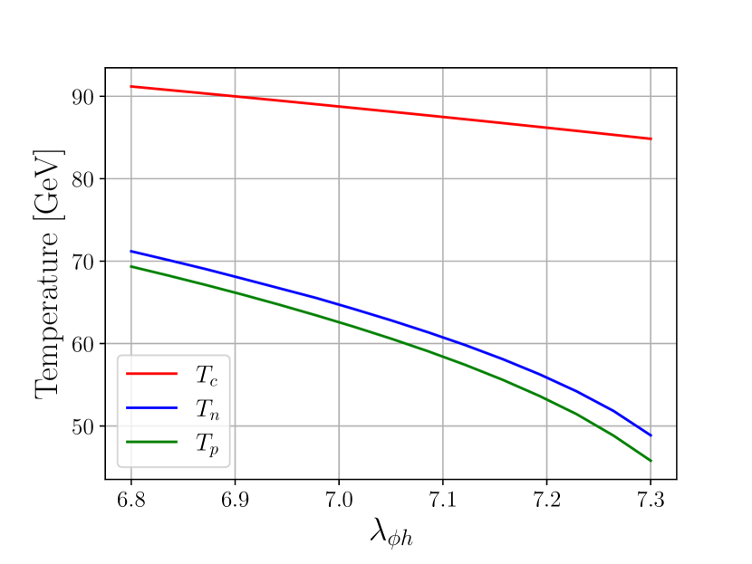
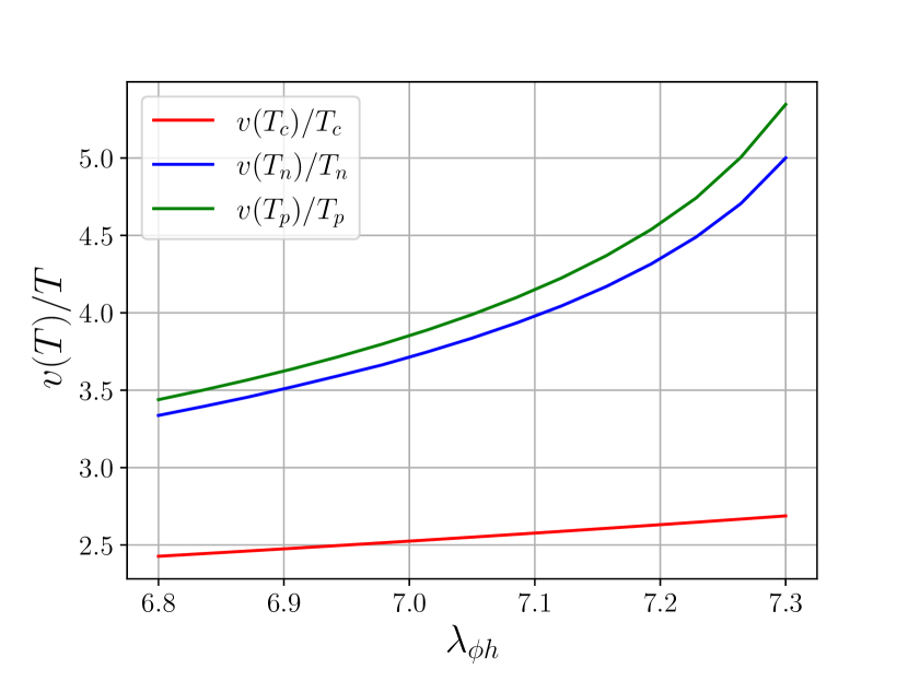
Figure 10: Phase transition parameters as functions of $\lambda_{\phi h}$. Left: the critical, nucleation and percolation temperatures for different values of $\lambda_{\phi h}$. For the percolation temperature we choose $v_{w}=0.1$. Right: the wash-out parameters $v(T)/T$ for various temperatures as functions of $\lambda_{\phi h}$.

5.2 Bubble wall filtering during FOPT

As the particles gain mass inside the bubble, due to the energy conservation, only high-energy particles can pass through the bubbles walls and the others are reflected. The condition of penetration in the bubble wall frame reads Baker:2019ndr ; Chway:2019kft :

$$p_{z}^{w}>\sqrt{\Delta m_{i}^{2}}\,\,,$$ (80)

where $p_{z}^{w}$ is the particle $z$-direction momentum in the bubble wall frame, $\Delta m_{i}^{2}=(m_{i}^{\mathrm{in}})^{2}-(m_{i}^{\mathrm{out}})^{2}$ is the mass difference between the true and false vacuum where $m_{i}^{\mathrm{in}}$ is the particle mass in the true vacuum and $m_{i}^{\mathrm{out}}$ is the mass in the false vacuum Chao:2020adk which we will set to zero in this work.

The particle flux coming from the false vacuum per unit area and unit time can be written as Baker:2019ndr ; Chway:2019kft

$${J}_{i}^{w}=g_{i}\int\frac{d^{3}{p^{w}}}{(2\pi)^{3}}\frac{{p}_{z}^{w}}{\sqrt{({{p}^{w}})^{2}+(m_{i}^{\mathrm{out}})^{2}}}f_{i}^{\rm eq}\Theta\left({p}_{z}^{w}-\sqrt{\Delta m^{2}}\right)\,\,,$$ (81)

where $g_{i}$ is degrees of freedom of the particle. $p^{w}$ is the magnitude of the three-momentum of the particles. $f_{i}^{\rm eq}$ is the equilibrium distribution outside the bubble in the bubble wall frame,

$$f_{i}^{\rm eq}=\frac{1}{e^{\gamma_{w}\left(\sqrt{({{p}^{w}})^{2}+(m_{i}^{\mathrm{out}})^{2}}-v_{w}{p}_{z}^{w}\right)/T}\mp 1}\,\,,$$ (82)

where $\mp$ is for bosons and fermions respectively. $v_{w}$ is the bubble wall velocity and $\gamma_{w}=1/\sqrt{1-v_{w}^{2}}$ is its Lorentz boost factor. The particle number density inside the bubble $n_{i}^{\text{in }}$ in the bubble center frame can be written as

$$n_{i}^{\text{in }}=\frac{{J}_{i}^{w}}{\gamma_{w}v_{w}}\,\,.$$ (83)

Assuming the particles are massless in the false vacuum, we can integrate Eq. (81) analytically and get Chway:2019kft ; Jiang:2023nkj

$$n_{i}^{\text{in }}\simeq\frac{g_{i}T^{3}}{\gamma_{w}v_{w}}\left(\frac{\gamma_{w}\left(1-v_{w}\right)m_{i}^{\mathrm{in}}/T+1}{4\pi^{2}\gamma_{w}^{3}\left(1-v_{w}\right)^{2}}\right)e^{-\frac{\gamma_{w}\left(1-v_{w}\right)m_{i}^{\mathrm{in}}}{T}}\,\,,$$ (84)

where we have used Maxwell-Boltzmann approximation of DM distribution. One can see that as ${v}_{w}\rightarrow 1$, Eq. (84) approaches $n_{i}^{\mathrm{out}}=g_{i}T^{3}/\pi^{2}$, which is approximately the equilibrium number density for Boltzmann distribution outside the bubble. The fraction of particles $i$ that are trapped into the false vacuum is defined by

$$F_{i}^{\mathrm{trap}}=1-\frac{n_{i}^{\mathrm{in}}}{n_{i}^{\mathrm{out}}}\,\,.$$ (85)

In our case, complex scalars $\phi$ and $\phi^{\dagger}$ are trapped into the false vacuum due to the filtering effect. The symmetric part would annihilate away in terms of the process $\phi+\phi^{\dagger}\rightarrow h+h$, then the asymmetric part survives and composes the charge of gauged Q-balls. It can be easily seen that the penetrated particle number density is sensitive to the bubble wall velocity as it appears in the exponent of Eq. (84). The precise calculation of bubble wall velocity Moore:1995si ; Laurent:2022jrs ; Lewicki:2021pgr ; Wang:2020zlf ; Jiang:2022btc ; Dorsch:2021nje ; DeCurtis:2022hlx ; Ai:2023see is beyond the scope of this work and we set it as a free parameter.

5.3 Charge of Q-ball in the electroweak FOPT

We can define $T_{\star}$ as the temperature at which the false vacuum or old phase remnants can still form an infinitely connected “cluster”, just like the definition of percolation temperature Hong:2020est . The $T_{\star}$ satisfies $p(T_{\star})=1-p(T_{p})=0.29$ which corresponds to $I(T_{\star})=1.24$. $T_{\star}$ is the temperature when Q-balls start to form. Below the temperature $T_{\star}$, the false vacuum remnants formed during FOPT may further fragment into smaller pieces. Ultimately, these pieces would shrink into Q-balls if there exists a non-zero primordial charge asymmetry. We can define the critical radius, $r_{c}$, at which the remnant shrinks to an insignificant size before another true vacuum bubble form within it Krylov:2013qe . This means Hong:2020est

$$\Gamma\left(T_{*}\right)\left(\frac{4\pi}{3}r_{c}^{3}\right)\Delta t\sim 1\,\,.$$ (86)

where $\Delta t=r_{c}/v_{w}$ is the time cost for shrinking. The number density of the remnants $n_{\mathrm{Q}}^{\star}$ can be expressed as:

$$n_{\mathrm{Q}}^{\star}\simeq 0.29\left(\frac{3}{4\pi}\right)^{1/4}\left(\frac{\Gamma\left(T_{\star}\right)}{v_{w}}\right)^{3/4}\,\,,$$ (87)

since the condition $n_{\mathrm{Q}}^{\star}\left(\frac{4\pi}{3}r_{c}^{3}\right)=p(T_{\star})\simeq 0.29$.

The formation of Q-balls requires a nonzero conserved primordial charge which comes from the primordial DM asymmetry $\eta_{\phi}=(n_{\phi}-n_{\phi^{\dagger}})/s$. The entropy density $s=2\pi^{2}g_{\star}T^{3}/45$. If the DM asymmetry is produced by thermal freeze-out in the early Universe, it is bounded from above by the equilibrium value,

$$\eta_{\phi}\lesssim\eta_{\phi}^{\mathrm{eq}}=\frac{n_{\phi}^{\mathrm{eq}}(T)}{s(T)}\simeq 5.1\times 10^{-3}\times\left(\frac{108.75}{g_{\star}}\right)\,\,,$$ (88)

where we have used $n_{\phi}^{\mathrm{eq}}(T)=2\zeta(3)T^{3}/\pi^{2}$ with $\zeta(3)=1.20206$ being the value of Riemann zeta function $\zeta(s)$ at $s=3$. In order to overcome this constraint, we assume the DM is produced by some non-thermal processes like decay. In this work, we do not specify the origin of primordial charge of the complex scalar $\phi$. In the early Universe at higher temperature, new physical processes beyond the standard model may have occurred. The would-be Q-ball DM particles $\phi$ may have their own conserved charge and be created in asymmetric decays of heavier particles Kaplan:2009ag . For example, heavy Majorana neutrino could decay into a light fermion and a scalar, like $N\rightarrow\bar{\chi}+\phi$ and $N\rightarrow\chi+\phi^{\dagger}$ where $\chi$ is a fermion Falkowski:2011xh . Assuming the process is CP-violating, the decay rates of these two channels differentiate from each other at loop level (when the $\phi$ is the standard model Higgs and $\chi$ is leptons, this is the process of leptogenesis.). So the asymmetry between $\phi$ and $\phi^{\dagger}$ appears and is retained until the phase transition in this work. The large DM asymmetry can be discussed in a similar manner to the large lepton asymmetry in the leptogenesis scenarios. Recent measurement of ${}^{4}\mathrm{He}$ abundance coming from the EMPRESS experiment suggests a large degeneracy parameter of the electron neutrino Matsumoto:2022tlr ,

$$\xi_{e}=0.05_{-0.02}^{+0.03}\,\,.$$ (89)

Since the neutrino oscillations among three flavors, the neutrinos with three flavors have the same amount of asymmetry, and then the total lepton asymmetry reads,

$$\eta_{L}\equiv 3\frac{n_{\nu_{e}}-n_{\bar{\nu}_{e}}}{s}=3\frac{T^{3}\xi_{e}/6}{2\pi^{2}g_{BBN}T^{3}/45}\simeq 5.3\times 10^{-3}\,\,,$$ (90)

where $g_{BBN}=10.75$ is the relativistic degree of freedom at the epoch of big bang nucleosynthesis. The large lepton asymmetry may comes from the low scale leptogenesis Borah:2022uos ; ChoeJo:2023cnx , Affleck-Dine mechanism McDonald:1999in or L-ball decay Kawasaki:2022hvx .

In a remnant, the trapped Q-charge is given by $Q_{\star}=F_{\phi}^{\mathrm{trap}}\eta_{\phi}s_{\star}/{n_{\mathrm{Q}}^{\star}}$. In figure 11, we show the charge of the gauged Q-ball DM formed during the FOPT for different values of bubble wall velocities. We have chosen $\eta_{\phi}=\eta_{L}$. When $\lambda_{\phi h}$ is larger, both the $\Gamma(T_{\star})$ and the Q-ball number density are suppressed, so that the charge is larger at a given $\eta_{\phi}$.

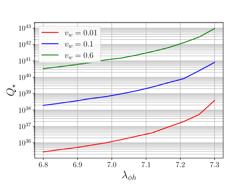
Figure 11: Charge of gauged Q-ball in electroweak FOPT. Here we choose $\eta_{\phi}=\eta_{L}$.

Since $n_{\mathrm{Q}}/s$ and $Q$ does not change in the adiabatic Universe, at present they are

$$n_{\mathrm{Q}}=\frac{n_{\mathrm{Q}}^{\star}}{s_{\star}}s_{0},\quad Q=Q_{\star}\,\,,$$ (91)

with $s_{0}=2891.2~{}\mathrm{cm}^{-3}$ being the entropy density in current time ParticleDataGroup:2018ovx .

We take the approximation $T_{\star}\approx T_{p}$ then the bounce action can be approximated written as Huber:2007vva

$$\frac{S_{3}(T_{\star})}{T_{\star}}\simeq 131-4\ln\left(\frac{T_{\star}}{100~{}\mathrm{GeV}}\right)-4\ln\left(\frac{\beta/H_{\star}}{100}\right)+3\ln v_{w}-2\ln\left(\frac{g_{\star}}{100}\right)\,\,,$$ (92)

where $\beta/H_{\star}=\left.\beta/H\right|_{T=T_{\star}}$. By approximately using $\Gamma(T_{\star})\approx T_{\star}^{4}e^{-S_{3}(T_{\star})/T_{\star}}$, then we get

$$Q=5.35\times 10^{36}F_{\phi}^{\mathrm{trap}}\left(\frac{v_{w}}{0.01}\right)^{3}\left(\frac{\eta_{\phi}}{\eta_{L}}\right)\left(\frac{100~{}\mathrm{GeV}}{T_{\star}}\right)^{3}\left(\frac{100}{\beta/H_{\star}}\right)^{3}\left(\frac{100}{g_{\star}}\right)^{1/2}\,\,.$$ (93)

In order to get stable gauged Q-ball with a given value of charge, we must impose $Q_{\mathrm{max}}>Q$, so the gauge coupling $\tilde{g}$ has to satisfy

$$\tilde{g}<1.28\times 10^{-18}\left(\frac{1}{F_{\phi}^{\mathrm{trap}}}\right)^{1/2}\left(\frac{0.01}{v_{w}}\right)^{3/2}\left(\frac{\eta_{L}}{\eta_{\phi}}\right)^{1/2}\left(\frac{T_{\star}}{100~{}\mathrm{GeV}}\right)^{3/2}\left(\frac{\beta/H_{\star}}{100}\right)^{3/2}\left(\frac{g_{\star}}{100}\right)^{1/4}\,\,.$$ (94)

5.4 Relic density of gauged Q-ball DM

The DM relic density can also have the contribution from the standard freeze-out, through the process $\phi+\phi^{\dagger}\leftrightarrow h+h$. The relic abundance reads,

$$\Omega_{\mathrm{freeze-out}}h_{100}^{2}\approx\frac{2.58\times 10^{-10}~{}\mathrm{GeV}^{-2}}{\langle\sigma_{\mathrm{anni}}v_{\mathrm{rel}}\rangle}\,\,,$$ (95)

where $\langle\sigma_{\mathrm{anni}}v_{\mathrm{rel}}\rangle$ is the annihilation cross section. $h_{100}=H_{0}/\left(100\mathrm{~{}km}\cdot\mathrm{s}^{-1}\cdot\mathrm{Mpc}^{-1}\right)=0.67$ where $H_{0}$ is the Hubble constant today Planck:2018vyg . The cross section of process $\phi+\phi^{\dagger}\leftrightarrow h+h$ reads $\frac{\lambda_{\phi h}^{2}}{64\pi m_{\phi}^{2}}\left(1-\frac{m_{h}^{2}}{m_{\phi}^{2}}\right)^{1/2}$ McDonald:1993ex . In our parameter space, where the $\lambda_{\phi h}$ is around 7, the relic abundance from freeze-out is approximately $\Omega_{\mathrm{freeze-out}}h_{100}^{2}\approx 2.35\times 10^{-4}$. So we can omit the DM produced from thermal freeze-out.

The DM relic density also receives the contribution from penetrated asymmetric components of DM particles which is given by the excess of $\phi$ over $\phi^{\dagger}$,

$$\Omega_{\mathrm{asymmetric}}h_{100}^{2}=(1-F_{\phi}^{\mathrm{trap}})\eta_{\phi}s_{0}m_{\phi}\,\,.$$ (96)

The relic density of Q-balls at present is

$$\Omega_{\mathrm{Q}}h_{100}^{2}=\frac{n_{\mathrm{Q}}E_{\mathrm{Q}}}{\rho_{\mathrm{c}}}h_{100}^{2}\,\,,$$ (97)

where $\rho_{\mathrm{c}}=3H_{0}^{2}M_{\mathrm{pl}}^{2}/(8\pi)$ is the critical energy density. We have found that, the gauged Q-ball is generally a mixed state of Eq. (56) and Eq. (58) as $0\leq\alpha B_{0}\rho_{b}\leq C_{2}$. So we can write down the energy of gauged Q-ball at a given charge,

$$E_{Q}\simeq\frac{\pi Q}{r_{\star}}+\frac{4\pi}{3}r_{\star}^{3}V_{0}+\frac{3}{20\pi}\frac{\tilde{g}^{2}Q^{2}}{r_{\star}}\,\,,$$ (98)

where $V_{0}=\frac{\lambda_{h}}{4}v_{0}^{4}$ is the potential difference between inside and outside of the gauged Q-balls at zero temperature. The first term on the right-side is the zero-point energy of the scalar particles, the second term is the vacuum volume energy inside the Q-ball and the third term is the electrostatic self energy. By minimizing this expression respect to $r_{\star}$, we obtain,

$$E_{Q}=\frac{4\pi}{3}\left(4V_{0}\right)^{1/4}Q^{3/4}\left(1+\frac{3\tilde{g}^{2}Q}{20\pi^{2}}\right)^{3/4}\,\,.$$ (99)

We can see that in the limit of zero gauge coupling

$$E_{Q}=\frac{4\pi}{3}\left(4V_{0}\right)^{1/4}Q^{3/4}=\frac{4\pi}{3}Q^{3/4}\lambda_{h}^{1/4}v_{0}\,\,,$$ (100)

which is just the energy of global Q-ball. By using $n_{\mathrm{Q}}=n_{\mathrm{Q}}^{\star}s_{0}/s_{\star}$ and $Q=Q_{\star}=F_{\phi}^{\mathrm{trap}}\eta_{\phi}s_{\star}/{n_{\mathrm{Q}}^{\star}}$, we finally arrive at the expression:

$$\Omega_{\mathrm{Q}}h_{100}^{2}$$ (101)

$$\simeq 2.81\times\left(\frac{s_{0}h_{100}^{2}}{\rho_{c}}\right)\left(\frac{\Gamma(T_{\star})}{v_{w}}\right)^{3/16}s_{\star}^{-1/4}(F_{\phi}^{\mathrm{trap}}\eta_{\phi})^{3/4}\lambda_{h}^{1/4}v_{0}\left(1+\frac{108^{1/4}\tilde{g}^{2}F_{\phi}^{\mathrm{trap}}\eta_{\phi}s_{\star}v_{w}^{3/4}}{5.4\pi^{7/4}\Gamma(T_{\star})^{3/4}}\right)\,\,,$$

the $\Gamma(T_{\star})$ can also be expanded by using $\Gamma(T_{\star})\approx T_{\star}^{4}e^{-S_{3}(T_{\star})/T_{\star}}$ and Eq. (92), but we keep the expression here to give more accurate results.

Although the expression hitherto is general, we apply these to the minimal SM plus singlet model. We choose $\lambda_{\phi h}=6.8$ for which $T_{n}=71.65~{}\mathrm{GeV}$ and $T_{p}=68.9~{}\mathrm{GeV}$. The number density of gauged Q-balls at production is $n_{Q}^{\star}\simeq 3.0\times 10^{-31}~{}\mathrm{GeV}^{-3}$. In this case, the value of $v(T_{p})/T_{p}$ is approximately 3.5 and there are still 50% of the DM particles trapping inside the false vacuum even at $v_{w}=0.6$. But it should be noted that in this case, the contribution from penetrated asymmetric DM will dominate, as can be seen in Eq. (96). This can be avoided in two ways. One way is to increase the phase transition strength and the corresponding $v(T)/T$ so there are little DM particles penetrating into the true vacuum, resulting $F_{\phi}^{\mathrm{trap}}\approx 1$. This can be achieved by introducing new freedoms beyond the standard model or considering dark FOPT instead of electroweak FOPT. The other way is model dependent: one can introduce new decay channels that penetrated $\phi$ could decay into dark radiation or SM leptons which can account for the lepton asymmetry. The decay process does not destroy the stability of Q-balls as long as $\pi/r_{\star}<m_{d}$ where $m_{d}$ is the mass of decay products. In this work we focus on the gauged Q-ball DM so we do not consider the penetrated asymmetric DM in details.

A strong FOPT requires large portal coupling $\lambda_{\phi h}=6.8$, and the validity of the perturbative analysis should be roughly smaller than 10 Curtin:2014jma . The condition of a strong FOPT leads to large deviation of triple Higgs coupling, which might be detected by the loop-induced $e^{+}e^{-}\to hZ$ process Huang:2015izx ; Huang:2016odd at future lepton colliders, such as FCC-ee, CEPC, and ILC.

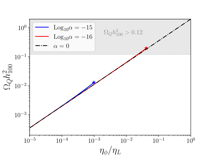
Figure 12: Q-ball relic density as function of DM asymmetry $\eta_{\phi}/\eta_{L}$ in the SM plus singlet model where $\lambda_{\phi h}=6.8$. We choose $v_{w}=0.01$. The star represents the value for the gauged Q-ball with maximal charge. The gray region represents the region where the DM is overproduced.

We show the gauged Q-ball DM relic density in figure 12. The colored star represents the value for the gauged Q-ball with maximal charge. The gray region represents the region where the DM is overproduced. We can see that due to the finiteness of the charge of gauged Q-balls, the gauged Q-balls can explain the whole DM at $v_{w}=0.01$ only when the rescaled gauge coupling $\alpha\lesssim 10^{-16}$. The DM relic density is slightly enhanced due to the extra electrostatic energy.

In table 1 we choose four benchmark points that satisfy the correct DM relic density and show the corresponding $F_{\phi}^{\mathrm{trap}}$ and $\eta_{\phi}/\eta_{L}$. Besides, we also show the fractional change in $Zh$ production relative to the SM prediction at one loop, $\delta\sigma_{Zh}$. We can see that the value of the required DM asymmetry $\eta_{\phi}$ is close to the lepton asymmetry $\eta_{L}$. This prompts us to speculate that they have the same origin. Actually, if the DM asymmetry comes from the process $N\rightarrow\bar{\chi}+\phi$ and $N\rightarrow\chi+\phi^{\dagger}$. We could assume the dark fermion $\chi$ is long-lived and decay suddenly into leptons after electroweak phase transition in order to avoid the electroweak sphaleron process. Then we expect the $\eta_{\phi}$ and $\eta_{L}$ is at the same order. The detailed model building is beyond the scope of this work and we leave this in our future studies.

	$\lambda_{\phi h}$	$T_{p}$ [GeV]	$\alpha_{p}$	$\beta/H_{p}$	$v_{w}$	$F_{\phi}^{\mathrm{trap}}$	$\eta_{\phi}/\eta_{L}$	$\delta\sigma_{Zh}$	GW
$BP_{1}$	6.8	69.8	0.12	540	$0.1$	0.932	0.48	-0.36%	${\color[rgb]{0,1,1}\bullet}$
$BP_{2}$	6.8	70.4	0.12	578	$0.6$	0.805	3.0	-0.36%	${\color[rgb]{1,0,1}\bullet}$
$BP_{3}$	7.0	63.0	0.15	372	$0.1$	0.965	3.4	-0.37%	${\color[rgb]{0,0,0}\bullet}$
$BP_{4}$	7.0	63.9	0.15	403	$0.6$	0.858	20.8	-0.37%	${\color[rgb]{1,0,0}\bullet}$

Table 1: Parameters of the model and phase transitions that satisfy $\Omega_{\mathrm{Q}}h_{100}^{2}\equiv 0.12$. We choose $\alpha=\tilde{g}/\sqrt{2\lambda_{h}}=10^{-18}$. $F_{\phi}^{\mathrm{trap}}$ is the fraction of DM particles which are trapped inside the false vacuum and $\eta_{\phi}/\eta_{L}$ is the DM asymmetry compared with the lepton asymmetry. $\delta\sigma_{Zh}$ is the fractional change in $Zh$ production relative to the SM prediction at one loop. GW represents the corresponding GW spectra in figure 14.

6 Constraints and detection of gauged Q-ball DM

6.1 Direct detection and astronomical constraints

We keep the gauged Q-ball DM mass and radius as free parameters to discuss its detection potential or constraints. The variation of gauged Q-ball DM mass and radius can be easily realize by varying the primordial DM asymmetry or the phase transition dynamics. The combined constraints of gauged Q-ball are shown in figure 13. As we have discussed in the previous sections, the size of the gauged Q-ball is restricted to be finite. The maximal charges or the maximal mass of gauged Q-ball DM at given gauge coupling are marked by the stars in figure 13. The gray region denotes the constraints from cosmic microwave background (CMB) which is affected by DM-baryon scattering Dvorkin:2013cea ; Jacobs:2014yca . DM cross sections have been probed by a variety of shallow and deep underground DM or repurposed experiments: XENON1T (orange) XENON:2018voc ; Clark:2020mna , Mica (purple) Price:1986ky ; Price:1988ge , Ohya (green) Bhoonah:2020fys . The Q-ball DM would transfer energy with other objects primarily through elastic scattering, approximately utilizing their geometric cross-section. When these cross-sections are sufficiently large, the resultant linear energy transfer might trigger observable phenomena. For example, if a macroscopic DM traverses compact objects such as white dwarfs or neutron stars and triggers thermonuclear runaway, this could potentially lead to a type IA supernova or superburst, respectively Graham:2018efk . The brown region represents constraints from superbursts in neutron stars SinghSidhu:2019tbr and the blue region from white dwarf becoming supernovae Graham:2018efk ; SinghSidhu:2019tbr . Combined all constraints in figure 13, one can see that the gauged Q-balls could be the DM candidate in a wide region of parameter space.

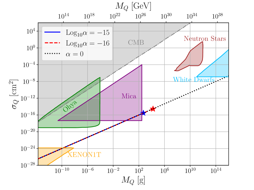
Figure 13: Combined constraints of direct detection and astronomical experiments on gauged Q-ball DM in the SM plus singlet model where $\lambda_{\phi h}=6.8$. The value corresponding to maximal charge is marked by a star.

6.2 Phase transition GW

The phase transition GW spectra comes from three sources of a strong FOPT: bubble collision, sound wave, and turbulence.

• Bubble collision
  The formula of phase transition GW from bubble collisions Huber:2008hg ; Caprini:2015zlo at the percolation temperature $T_{p}$ , reads:

  $$\Omega_{\mathrm{co}}h_{100}^{2}\simeq 1.67\times 10^{-5}\left(\frac{H_{p}}{\beta}\right)^{2}\left(\frac{\kappa_{h}\alpha_{p}}{1+\alpha_{p}}\right)^{2}\left(\frac{100}{g_{\star}}\right)^{1/3}\frac{0.11v_{w}^{3}}{0.42+v_{w}^{2}}\frac{3.8\left(f/f_{\mathrm{co}}\right)^{2.8}}{1+2.8\left(f/f_{\mathrm{co}}\right)^{3.8}}\,\,,$$ (102)

  where $\beta/H_{p}$ and $\alpha_{p}$ are defined at percolation temperature, respectively. $\kappa_{h}$ represents the fraction of vacuum energy converted into the scalar field’s gradient energy. $f_{\mathrm{co}}$ is the peak frequency of bubble collision:

  $$f_{\mathrm{co}}\simeq 1.65\times 10^{-5}\mathrm{~{}Hz}\left(\frac{\beta}{H_{p}}\right)\left(\frac{0.62}{1.8-0.1v_{w}+v_{w}^{2}}\right)\left(\frac{T_{p}}{100~{}\mathrm{GeV}}\right)\left(\frac{g_{\star}}{100}\right)^{1/6}\,\,.$$ (103)

• Sound wave
  The contribution from sound waves could be more significant. The formula GW spectrum from sound waves is Hindmarsh:2017gnf :

  $$\Omega_{\mathrm{sw}}h_{100}^{2}\simeq 2.65\times 10^{-6}\Upsilon_{\mathrm{sw}}\left(\frac{H_{p}}{\beta}\right)\left(\frac{\kappa_{v}\alpha_{p}}{1+\alpha_{p}}\right)^{2}\left(\frac{100}{g_{\star}}\right)^{1/3}v_{w}\left(f/f_{\mathrm{sw}}\right)^{3}\left(\frac{7}{4+3\left(f/f_{\mathrm{sw}}\right)^{2}}\right)^{7/2}\,\,,$$ (104)

  where $\kappa_{v}$ reflects the fraction of vacuum energy that transfers into the fluid’s bulk motion. The peak frequency of sound waves processes is:

  $$f_{\mathrm{sw}}\simeq 1.9\times 10^{-5}\mathrm{~{}Hz}\frac{1}{v_{w}}\left(\frac{\beta}{H_{p}}\right)\left(\frac{T_{p}}{100~{}\mathrm{GeV}}\right)\left(\frac{g_{\star}}{100}\right)^{1/6}\,\,.$$ (105)

  $\Upsilon_{\mathrm{sw}}$ is the suppression factor of the short period of the sound wave,

  $$\Upsilon_{\mathrm{sw}}=\left(1-\frac{1}{\sqrt{1+2\tau_{\mathrm{sw}}H_{p}}}\right)\,\,,$$ (106)

  where

  $$\tau_{\mathrm{sw}}H_{p}\approx(8\pi)^{\frac{1}{3}}\frac{v_{w}(H_{p}/\beta)}{\sqrt{3\kappa_{v}\alpha_{p}/(4+4\alpha_{p})}}\,\,.$$ (107)

• Turbulence
  The formula of the GW spectrum from turbulence is Binetruy:2012ze :

  $$\Omega_{\mathrm{turb}}h_{100}^{2}\simeq 3.35\times 10^{-4}\left(\frac{H_{p}v_{w}}{\beta}\right)\left(\frac{\kappa_{\mathrm{turb}}\alpha_{p}}{1+\alpha_{p}}\right)^{3/2}\left(\frac{100}{g_{\star}}\right)^{1/3}\frac{\left(f/f_{\text{turb }}\right)^{3}}{\left(1+f/f_{\text{turb }}\right)^{11/3}\left(1+8\pi f/H_{p}\right)}\,\,,$$ (108)

  note that $H_{p}$ is the Hubble rate at $T_{p}$:

  $$H_{p}=1.65\times 10^{-5}~{}\mathrm{Hz}\left(\frac{T_{p}}{100~{}\mathrm{GeV}}\right)\left(\frac{g_{\star}}{100}\right)^{1/6}\,\,,$$ (109)

  and the peak frequency of turbulence processes is :

  $$f_{\text{turb }}\simeq 2.7\times 10^{-5}\mathrm{~{}Hz}\frac{1}{v_{w}}\left(\frac{\beta}{H_{p}}\right)\left(\frac{T_{p}}{100~{}\mathrm{GeV}}\right)\left(\frac{g_{\star}}{100}\right)^{1/6}\,\,.$$ (110)

  $\kappa_{\mathrm{turb}}$ represents the efficiency of vacuum energy being converted into turbulent flow:

  $$\kappa_{\text{turb }}=\tilde{\epsilon}\kappa_{v}\,\,,$$ (111)

  where the $\tilde{\epsilon}$ is set to $0.1$.

The total contribution to the GW spectra can be calculated by summing these individual contributions:

$$\Omega_{\mathrm{GW}}h_{100}^{2}=\Omega_{\mathrm{co}}h_{100}^{2}+\Omega_{\mathrm{sw}}h_{100}^{2}+\Omega_{\mathrm{turb}}h_{100}^{2}\,\,.$$ (112)

We show the GW spectra $\Omega_{\mathrm{GW}}h_{100}^{2}$ for four benchmark points in figure 14. These four benchmark points are shown in Table 1. We choose $\lambda_{\phi h}=6.8$ and $7.0$ and for each value of $\lambda_{\phi h}$ we choose two bubble wall velocities $v_{w}=0.1,0.6$. The colored regions represent the sensitivity curves for future GW detectors LISA LISA:2017pwj and TianQin TianQin:2015yph ; Liang:2022ufy with the signal-to-noise ratio (SNR) about 5. We can see that the LISA and TianQin could detect this new DM mechanism when the bubble wall velocity is relatively large. Taiji Hu:2017mde , BBO Corbin:2005ny , DECIGO Seto:2001qf , Ultimate-DECIGO Kudoh:2005as could also detect this new DM mechanism by GW signals.

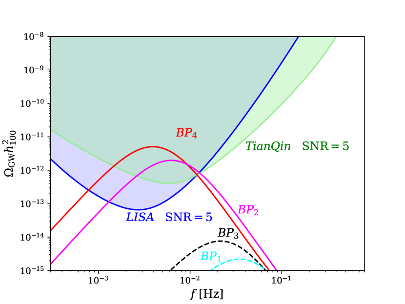
Figure 14: GW spectra for four benchmark points in Table 1. The future GW detectors LISA LISA:2017pwj , TianQin TianQin:2015yph ; Liang:2022ufy could detect $BP_{2}$ and $BP_{4}$ whose bubble wall velocities are relatively large.

7 Discussion and conclusion

In this work, we have systematically discussed the gauged Q-ball DM formed during a FOPT. We have investigated the stability of gauged Q-balls, including quantum stability, stress stability, fission stability, and classical stability. Different from the global Q-balls, the gauge interaction restricts the size of the stable gauged Q-balls. For a given value of the gauge coupling, the stable gauged Q-balls can only be realized in the region of charge $Q_{s}<Q<Q_{\mathrm{max}}$. The upper limit $Q_{\mathrm{max}}$ and lower limit $Q_{s}$ mainly comes from the stress stability and quantum stability criterion respectively. By using the thin-wall approximation, we show that the piecewise model can describe the basic properties of gauged Q-balls in FLSM model well. Based on this, we further give an approximately analytic evaluation of $Q_{\mathrm{max}}$ by using the mapping method. We find the maximal charge is approximately $Q_{\mathrm{max}}\propto\tilde{g}^{-2}$ where $\tilde{g}$ is the gauge coupling of the dark $U(1)$ symmetry. The constraint on the value of gauge coupling $\tilde{g}$ is given by Eq. (94) if the gauged Q-balls are produced by the FOPT. We discuss the relic density of gauged Q-ball DM formed during electroweak FOPT. Even in the minimal SM plus singlet electroweak FOPT model, the gauged Q-balls can comprise all the observed DM. And we have found that in order to satisfy the relic abundance of DM, the original DM asymmetry surprisingly coincides with the observed large lepton number asymmetry. The charge and mass of gauged Q-ball DM can be varied by modifying the phase transition dynamics or the primordial DM asymmetry. Besides, we give combined constraints on the gauged Q-ball DM from DM direct detection (Mica, XENON1T, Ohya), and astronomical observations (CMB, neutron stars, white dwarfs). The formation process of gauged Q-ball DM during FOPT also provides phase transition GW signals which could be detected by future GW experiments such as LISA, TianQin, and Taiji. The phase transition dynamics in the early universe provides new formation mechanisms of various soliton DM or dynamical DM. For example, it is reasonable to discuss other species of soliton DM formed during FOPT, such as gauged Fermi-ball DM. The configuration of the Fermi-ball is different from the Q-ball because of the extra Fermi-gas degeneracy pressure. We leave these in our future works.

Acknowledgements:

The authors thank Emin Nugaev, Julian Heeck, Michael Baker, Kiyoharu Kawana, Mikhail Smolyakov, Mikheil Sokhashvili, Yakov M. Shnir, Dmitry Levkov, Muhammad Fakhri Afif, Chris Verhaaren, Rebecca Riley, Sida Lu, Bingrong Yu, Jiahang Hu for helpful correspondence. This work was supported by the National Natural Science Foundation of China (NNSFC) under Grant No. 12205387, by Guangdong Major Project of Basic and Applied Basic Research (Grant No. 2019B030302001), and by KIAS Individual Grants under Grants No. PG021403 (PK).

References

- (1) G. Bertone and D. Hooper, History of dark matter, Rev. Mod. Phys. 90 (2018) 045002 [1605.04909].
- (2) A. Boveia et al., Snowmass 2021 Dark Matter Complementarity Report, 2211.07027.
- (3) A. Boveia et al., Snowmass 2021 Cross Frontier Report: Dark Matter Complementarity (Extended Version), 2210.01770.
- (4) J. Cooley et al., Report of the Topical Group on Particle Dark Matter for Snowmass 2021, 2209.07426.
- (5) S. Baek, P. Ko and P. Wu, Top-philic Scalar Dark Matter with a Vector-like Fermionic Top Partner, JHEP 10 (2016) 117 [1606.00072].
- (6) S. Baek, P. Ko and P. Wu, Heavy quark-philic scalar dark matter with a vector-like fermion portal, JCAP 07 (2018) 008 [1709.00697].
- (7) T. Abe, J. Kawamura, S. Okawa and Y. Omura, Dark matter physics, flavor physics and LHC constraints in the dark matter model with a bottom partner, JHEP 03 (2017) 058 [1612.01643].
- (8) S. Khan, J. Kim and P. Ko, Interplay between Higgs inflation and dark matter models with dark gauge symmetry, 2309.07839.
- (9) H. Baer, K.-Y. Choi, J.E. Kim and L. Roszkowski, Dark matter production in the early Universe: beyond the thermal WIMP paradigm, Phys. Rept. 555 (2015) 1 [1407.0017].
- (10) T. Lin, Dark matter models and direct detection, PoS 333 (2019) 009 [1904.07915].
- (11) S. Baek, P. Ko and W.-I. Park, Hidden sector monopole, vector dark matter and dark radiation with Higgs portal, JCAP 10 (2014) 067 [1311.1035].
- (12) A. Derevianko and M. Pospelov, Hunting for topological dark matter with atomic clocks, Nature Phys. 10 (2014) 933 [1311.1244].
- (13) E. Witten, Cosmic Separation of Phases, Phys. Rev. D 30 (1984) 272.
- (14) E. Krylov, A. Levin and V. Rubakov, Cosmological phase transition, baryon asymmetry and dark matter Q-balls, Phys. Rev. D 87 (2013) 083528 [1301.0354].
- (15) F.P. Huang and C.S. Li, Probing the baryogenesis and dark matter relaxed in phase transition by gravitational waves and colliders, Phys. Rev. D 96 (2017) 095028 [1709.09691].
- (16) S. Jiang, A. Yang, J. Ma and F.P. Huang, Implication of nano-Hertz stochastic gravitational wave on dynamical dark matter through a dark first-order phase transition, Class. Quant. Grav. 41 (2024) 065009 [2306.17827].
- (17) J.-P. Hong, S. Jung and K.-P. Xie, Fermi-ball dark matter from a first-order phase transition, Phys. Rev. D 102 (2020) 075028 [2008.04430].
- (18) K. Griest and M. Kamionkowski, Unitarity Limits on the Mass and Radius of Dark Matter Particles, Phys. Rev. Lett. 64 (1990) 615.
- (19) M.J. Baker, J. Kopp and A.J. Long, Filtered Dark Matter at a First Order Phase Transition, Phys. Rev. Lett. 125 (2020) 151102 [1912.02830].
- (20) D. Chway, T.H. Jung and C.S. Shin, Dark matter filtering-out effect during a first-order phase transition, Phys. Rev. D 101 (2020) 095019 [1912.04238].
- (21) G. Rosen, Particlelike Solutions to Nonlinear Complex Scalar Field Theories with Positive-Definite Energy Densities, J. Math. Phys. 9 (1968) 996.
- (22) S.R. Coleman, Q-balls, Nucl. Phys. B 262 (1985) 263.
- (23) K.-M. Lee, J.A. Stein-Schabes, R. Watkins and L.M. Widrow, Gauged q Balls, Phys. Rev. D 39 (1989) 1665.
- (24) G. Rosen, Charged Particlelike Solutions to Nonlinear Complex Scalar Field Theories, J. Math. Phys. 9 (1968) 999.
- (25) C.H. Lee and S.U. Yoon, Existence and stability of gauged nontopological solitons, Mod. Phys. Lett. A 6 (1991) 1479.
- (26) R. Friedberg, T.D. Lee and A. Sirlin, A Class of Scalar-Field Soliton Solutions in Three Space Dimensions, Phys. Rev. D 13 (1976) 2739.
- (27) H. Arodz and J. Lis, Compact Q-balls and Q-shells in a scalar electrodynamics, Phys. Rev. D 79 (2009) 045002 [0812.3284].
- (28) V. Benci and D. Fortunato, On the existence of stable charged Q-balls, J. Math. Phys. 52 (2011) 093701 [1011.5044].
- (29) V. Benci and D. Fortunato, Hylomorphic solitons and charged Q-balls: Existence and stability, Chaos Solitons Fractals 58 (2014) 1 [1212.3236].
- (30) V. Dzhunushaliev and K.G. Zloshchastiev, Singularity-free model of electric charge in physical vacuum: Non-zero spatial extent and mass generation, Central Eur. J. Phys. 11 (2013) 325 [1204.6380].
- (31) I.E. Gulamov, E.Y. Nugaev and M.N. Smolyakov, Theory of gauged Q-balls revisited, Phys. Rev. D 89 (2014) 085006 [1311.0325].
- (32) I.E. Gulamov, E.Y. Nugaev, A.G. Panin and M.N. Smolyakov, Some properties of U(1) gauged Q-balls, Phys. Rev. D 92 (2015) 045011 [1506.05786].
- (33) E.Y. Nugaev and A.V. Shkerin, Review of Nontopological Solitons in Theories with -Symmetry, J. Exp. Theor. Phys. 130 (2020) 301 [1905.05146].
- (34) A. Kusenko, Solitons in the supersymmetric extensions of the standard model, Phys. Lett. B 405 (1997) 108 [hep-ph/9704273].
- (35) A. Kusenko and M.E. Shaposhnikov, Supersymmetric Q balls as dark matter, Phys. Lett. B 418 (1998) 46 [hep-ph/9709492].
- (36) S. Kasuya, M. Kawasaki and M. Yamada, Revisiting the gravitino dark matter and baryon asymmetry from Q-ball decay in gauge mediation, Phys. Lett. B 726 (2013) 1 [1211.4743].
- (37) J.-P. Hong and M. Kawasaki, New type of charged Q -ball dark matter in gauge mediated SUSY breaking models, Phys. Rev. D 95 (2017) 123532 [1702.00889].
- (38) J.-P. Hong, M. Kawasaki and M. Yamada, Charged Q-ball Dark Matter from and direction, JCAP 08 (2016) 053 [1604.04352].
- (39) LISA collaboration, Laser Interferometer Space Antenna, 1702.00786.
- (40) TianQin collaboration, TianQin: a space-borne gravitational wave detector, Class. Quant. Grav. 33 (2016) 035010 [1512.02076].
- (41) Z.-C. Liang, Z.-Y. Li, J. Cheng, E.-K. Li, J.-d. Zhang and Y.-M. Hu, Impact of combinations of time-delay interferometry channels on stochastic gravitational wave background detection, Phys. Rev. D 107 (2023) 083033 [2212.02852].
- (42) W.-R. Hu and Y.-L. Wu, The Taiji Program in Space for gravitational wave physics and the nature of gravity, Natl. Sci. Rev. 4 (2017) 685.
- (43) V. Corbin and N.J. Cornish, Detecting the cosmic gravitational wave background with the big bang observer, Class. Quant. Grav. 23 (2006) 2435 [gr-qc/0512039].
- (44) N. Seto, S. Kawamura and T. Nakamura, Possibility of direct measurement of the acceleration of the universe using 0.1-Hz band laser interferometer gravitational wave antenna in space, Phys. Rev. Lett. 87 (2001) 221103 [astro-ph/0108011].
- (45) H. Kudoh, A. Taruya, T. Hiramatsu and Y. Himemoto, Detecting a gravitational-wave background with next-generation space interferometers, Phys. Rev. D 73 (2006) 064006 [gr-qc/0511145].
- (46) J. Heeck and M. Sokhashvili, Revisiting the Friedberg–Lee–Sirlin soliton model, Eur. Phys. J. C 83 (2023) 526 [2303.09566].
- (47) E. Pontón, Y. Bai and B. Jain, Electroweak Symmetric Dark Matter Balls, JHEP 09 (2019) 011 [1906.10739].
- (48) V. Loiko and Y. Shnir, Q-balls in the gauged Friedberg-Lee-Sirlin model, Phys. Lett. B 797 (2019) 134810 [1906.01943].
- (49) V. Loiko and Y. Shnir, Q-ball stress stability criterion in U(1) gauged scalar theories, Phys. Rev. D 106 (2022) 045021 [2207.02646].
- (50) M.P. Kinach and M.W. Choptuik, Dynamical evolution of U(1) gauged Q-balls in axisymmetry, Phys. Rev. D 107 (2023) 035022 [2211.11198].
- (51) W.H. Press, S.A. Teukolsky, W.T. Vetterling and B.P. Flannery, Numerical Recipes 3rd Edition: The Art of Scientific Computing, Cambridge University Press, New York, NY, USA, 3 ed. (2007).
- (52) H.-K. Guo, K. Sinha, C. Sun, J. Swaim and D. Vagie, Two-scalar Bose-Einstein condensates: from stars to galaxies, JCAP 10 (2021) 028 [2010.15977].
- (53) A.G. Cohen, S.R. Coleman, H. Georgi and A. Manohar, The Evaporation of Balls, Nucl. Phys. B 272 (1986) 301.
- (54) M. Kawasaki and M. Yamada, ball Decay Rates into Gravitinos and Quarks, Phys. Rev. D 87 (2013) 023517 [1209.5781].
- (55) J.-P. Hong and M. Kawasaki, Gauged Q-ball Decay Rates into Fermions, Phys. Rev. D 96 (2017) 103526 [1706.01651].
- (56) M. Laue, Zur Dynamik der Relativitätstheorie, Annalen Phys. 340 (1911) 524.
- (57) I. Bialynicki-Birula, Simple relativistic model of a finite size particle, Phys. Lett. A 182 (1993) 346 [nucl-th/9306006].
- (58) M.V. Polyakov, Generalized parton distributions and strong forces inside nucleons and nuclei, Phys. Lett. B 555 (2003) 57 [hep-ph/0210165].
- (59) M. Mai and P. Schweitzer, Energy momentum tensor, stability, and the D-term of Q-balls, Phys. Rev. D 86 (2012) 076001 [1206.2632].
- (60) M.V. Polyakov and P. Schweitzer, Forces inside hadrons: pressure, surface tension, mechanical radius, and all that, Int. J. Mod. Phys. A 33 (2018) 1830025 [1805.06596].
- (61) I.A. Perevalova, M.V. Polyakov and P. Schweitzer, On LHCb pentaquarks as a baryon-(2S) bound state: prediction of isospin- pentaquarks with hidden charm, Phys. Rev. D 94 (2016) 054024 [1607.07008].
- (62) K.N. Anagnostopoulos, M. Axenides, E.G. Floratos and N. Tetradis, Large gauged Q balls, Phys. Rev. D 64 (2001) 125006 [hep-ph/0109080].
- (63) H. Ishihara and T. Ogawa, Charge Screened Nontopological Solitons in a Spontaneously Broken U(1) Gauge Theory, PTEP 2019 (2019) 021B01 [1811.10894].
- (64) A.G. Panin and M.N. Smolyakov, Problem with classical stability of U(1) gauged Q-balls, Phys. Rev. D 95 (2017) 065006 [1612.00737].
- (65) T.D. Lee and Y. Pang, Nontopological solitons, Phys. Rept. 221 (1992) 251.
- (66) N.G. Vakhitov and A.A. Kolokolov, Stationary solutions of the wave equation in the medium with nonlinearity saturation, .
- (67) V.G. Makhankov, Dynamics of classical solitons (in non-integrable systems), Physics Reports 35 (1978) 1.
- (68) D. Levkov, E. Nugaev and A. Popescu, The fate of small classically stable Q-balls, JHEP 12 (2017) 131 [1711.05279].
- (69) J. Heeck, A. Rajaraman, R. Riley and C.B. Verhaaren, Mapping Gauged Q-Balls, Phys. Rev. D 103 (2021) 116004 [2103.06905].
- (70) I.E. Gulamov, E.Y. Nugaev and M.N. Smolyakov, Analytic -ball solutions and their stability in a piecewise parabolic potential, Phys. Rev. D 87 (2013) 085043 [1303.1173].
- (71) E. Kim and E. Nugaev, Effectively flat potential in the Friedberg-Lee-Sirlin model, 2309.09661.
- (72) J. Heeck, A. Rajaraman, R. Riley and C.B. Verhaaren, Understanding Q-Balls Beyond the Thin-Wall Limit, Phys. Rev. D 103 (2021) 045008 [2009.08462].
- (73) J.R. Espinosa and M. Quiros, The Electroweak phase transition with a singlet, Phys. Lett. B 305 (1993) 98 [hep-ph/9301285].
- (74) P. Bandyopadhyay and S. Jangid, Discerning singlet and triplet scalars at the electroweak phase transition and gravitational wave, Phys. Rev. D 107 (2023) 055032 [2111.03866].
- (75) L. Dolan and R. Jackiw, Symmetry Behavior at Finite Temperature, Phys. Rev. D 9 (1974) 3320.
- (76) A. Salvio, A. Strumia, N. Tetradis and A. Urbano, On gravitational and thermal corrections to vacuum decay, JHEP 09 (2016) 054 [1608.02555].
- (77) M.S. Turner, E.J. Weinberg and L.M. Widrow, Bubble nucleation in first order inflation and other cosmological phase transitions, Phys. Rev. D 46 (1992) 2384.
- (78) J. Ellis, M. Lewicki and J.M. No, On the Maximal Strength of a First-Order Electroweak Phase Transition and its Gravitational Wave Signal, JCAP 04 (2019) 003 [1809.08242].
- (79) A. Megevand and S. Ramirez, Bubble nucleation and growth in very strong cosmological phase transitions, Nucl. Phys. B 919 (2017) 74 [1611.05853].
- (80) A. Kobakhidze, C. Lagger, A. Manning and J. Yue, Gravitational waves from a supercooled electroweak phase transition and their detection with pulsar timing arrays, Eur. Phys. J. C 77 (2017) 570 [1703.06552].
- (81) J. Ellis, M. Lewicki and J.M. No, Gravitational waves from first-order cosmological phase transitions: lifetime of the sound wave source, JCAP 07 (2020) 050 [2003.07360].
- (82) X. Wang, F.P. Huang and X. Zhang, Phase transition dynamics and gravitational wave spectra of strong first-order phase transition in supercooled universe, JCAP 05 (2020) 045 [2003.08892].
- (83) C.L. Wainwright, CosmoTransitions: Computing Cosmological Phase Transition Temperatures and Bubble Profiles with Multiple Fields, Comput. Phys. Commun. 183 (2012) 2006 [1109.4189].
- (84) W. Chao, X.-F. Li and L. Wang, Filtered pseudo-scalar dark matter and gravitational waves from first order phase transition, JCAP 06 (2021) 038 [2012.15113].
- (85) S. Jiang, F.P. Huang and C.S. Li, Hydrodynamic effects on the filtered dark matter produced by a first-order phase transition, Phys. Rev. D 108 (2023) 063508 [2305.02218].
- (86) G.D. Moore and T. Prokopec, How fast can the wall move? A Study of the electroweak phase transition dynamics, Phys. Rev. D 52 (1995) 7182 [hep-ph/9506475].
- (87) B. Laurent and J.M. Cline, First principles determination of bubble wall velocity, Phys. Rev. D 106 (2022) 023501 [2204.13120].
- (88) M. Lewicki, M. Merchand and M. Zych, Electroweak bubble wall expansion: gravitational waves and baryogenesis in Standard Model-like thermal plasma, JHEP 02 (2022) 017 [2111.02393].
- (89) X. Wang, F.P. Huang and X. Zhang, Bubble wall velocity beyond leading-log approximation in electroweak phase transition, 2011.12903.
- (90) S. Jiang, F.P. Huang and X. Wang, Bubble wall velocity during electroweak phase transition in the inert doublet model, Phys. Rev. D 107 (2023) 095005 [2211.13142].
- (91) G.C. Dorsch, S.J. Huber and T. Konstandin, A sonic boom in bubble wall friction, JCAP 04 (2022) 010 [2112.12548].
- (92) S. De Curtis, L.D. Rose, A. Guiggiani, A.G. Muyor and G. Panico, Bubble wall dynamics at the electroweak phase transition, JHEP 03 (2022) 163 [2201.08220].
- (93) W.-Y. Ai, B. Laurent and J. van de Vis, Model-independent bubble wall velocities in local thermal equilibrium, JCAP 07 (2023) 002 [2303.10171].
- (94) D.E. Kaplan, M.A. Luty and K.M. Zurek, Asymmetric Dark Matter, Phys. Rev. D 79 (2009) 115016 [0901.4117].
- (95) A. Falkowski, J.T. Ruderman and T. Volansky, Asymmetric Dark Matter from Leptogenesis, JHEP 05 (2011) 106 [1101.4936].
- (96) A. Matsumoto et al., EMPRESS. VIII. A New Determination of Primordial He Abundance with Extremely Metal-poor Galaxies: A Suggestion of the Lepton Asymmetry and Implications for the Hubble Tension, Astrophys. J. 941 (2022) 167 [2203.09617].
- (97) D. Borah and A. Dasgupta, Large neutrino asymmetry from TeV scale leptogenesis, Phys. Rev. D 108 (2023) 035015 [2206.14722].
- (98) Y. ChoeJo, K. Enomoto, Y. Kim and H.-S. Lee, Second leptogenesis: Unraveling the baryon-lepton asymmetry discrepancy, JHEP 03 (2024) 003 [2311.16672].
- (99) J. McDonald, Naturally large cosmological neutrino asymmetries in the MSSM, Phys. Rev. Lett. 84 (2000) 4798 [hep-ph/9908300].
- (100) M. Kawasaki and K. Murai, Lepton asymmetric universe, JCAP 08 (2022) 041 [2203.09713].
- (101) Particle Data Group collaboration, Review of Particle Physics, Phys. Rev. D 98 (2018) 030001.
- (102) S.J. Huber and T. Konstandin, Production of gravitational waves in the nMSSM, JCAP 05 (2008) 017 [0709.2091].
- (103) Planck collaboration, Planck 2018 results. VI. Cosmological parameters, Astron. Astrophys. 641 (2020) A6 [1807.06209].
- (104) J. McDonald, Gauge singlet scalars as cold dark matter, Phys. Rev. D 50 (1994) 3637 [hep-ph/0702143].
- (105) D. Curtin, P. Meade and C.-T. Yu, Testing Electroweak Baryogenesis with Future Colliders, JHEP 11 (2014) 127 [1409.0005].
- (106) F.P. Huang, P.-H. Gu, P.-F. Yin, Z.-H. Yu and X. Zhang, Testing the electroweak phase transition and electroweak baryogenesis at the LHC and a circular electron-positron collider, Phys. Rev. D 93 (2016) 103515 [1511.03969].
- (107) F.P. Huang, Y. Wan, D.-G. Wang, Y.-F. Cai and X. Zhang, Hearing the echoes of electroweak baryogenesis with gravitational wave detectors, Phys. Rev. D 94 (2016) 041702 [1601.01640].
- (108) C. Dvorkin, K. Blum and M. Kamionkowski, Constraining Dark Matter-Baryon Scattering with Linear Cosmology, Phys. Rev. D 89 (2014) 023519 [1311.2937].
- (109) D.M. Jacobs, G.D. Starkman and B.W. Lynn, Macro Dark Matter, Mon. Not. Roy. Astron. Soc. 450 (2015) 3418 [1410.2236].
- (110) XENON collaboration, Dark Matter Search Results from a One Ton-Year Exposure of XENON1T, Phys. Rev. Lett. 121 (2018) 111302 [1805.12562].
- (111) M. Clark, A. Depoian, B. Elshimy, A. Kopec, R.F. Lang, S. Li et al., Direct Detection Limits on Heavy Dark Matter, Phys. Rev. D 102 (2020) 123026 [2009.07909].
- (112) P.B. Price and M.H. Salamon, Search for Supermassive Magnetic Monopoles Using Mica Crystals, Phys. Rev. Lett. 56 (1986) 1226.
- (113) P.B. Price, Limits on Contribution of Cosmic Nuclearites to Galactic Dark Matter, Phys. Rev. D 38 (1988) 3813.
- (114) A. Bhoonah, J. Bramante, B. Courtman and N. Song, Etched plastic searches for dark matter, Phys. Rev. D 103 (2021) 103001 [2012.13406].
- (115) P.W. Graham, R. Janish, V. Narayan, S. Rajendran and P. Riggins, White Dwarfs as Dark Matter Detectors, Phys. Rev. D 98 (2018) 115027 [1805.07381].
- (116) J. Singh Sidhu and G.D. Starkman, Reconsidering astrophysical constraints on macroscopic dark matter, Phys. Rev. D 101 (2020) 083503 [1912.04053].
- (117) S.J. Huber and T. Konstandin, Gravitational Wave Production by Collisions: More Bubbles, JCAP 09 (2008) 022 [0806.1828].
- (118) C. Caprini et al., Science with the space-based interferometer eLISA. II: Gravitational waves from cosmological phase transitions, JCAP 04 (2016) 001 [1512.06239].
- (119) M. Hindmarsh, S.J. Huber, K. Rummukainen and D.J. Weir, Shape of the acoustic gravitational wave power spectrum from a first order phase transition, Phys. Rev. D 96 (2017) 103520 [1704.05871].
- (120) P. Binetruy, A. Bohe, C. Caprini and J.-F. Dufaux, Cosmological Backgrounds of Gravitational Waves and eLISA/NGO: Phase Transitions, Cosmic Strings and Other Sources, JCAP 06 (2012) 027 [1201.0983].