Violation of Bell inequalities in an analogue black hole

Abstract

Signals of entanglement and nonlocality are quantitatively evaluated at zero and finite temperature in an analogue black hole realized in the flow of a quasi one-dimensional Bose-Einstein condensate. The violation of Lorentz invariance inherent to this analog system opens the prospect to observe 3-mode quantum correlations and we study the corresponding violation of bipartite and tripartite Bell inequalities. It is shown that the long wavelength modes of the system are maximally entangled, in the sense that they realize a superposition of continuous variable versions of Greenberger-Horne-Zeilinger states whose entanglement resists partial tracing.

I Introduction

The domain of analog gravity aims at providing laboratory models for gaining insight on general relativity phenomena that cannot be directly observed in the usual gravitational context or for which there exists no complete theoretical framework. Two such phenomena are black hole superradiance [1, 2, 3] and Hawking radiation [4, 5]. In that context, the most successful analogous experimental platforms have been surface gravity [6, 7, 8, 9, 10] and acoustic [11] waves, nonlinear optical systems [12, 13], cavity polaritons [14, 15, 16] and Bose-Einstein condendates (BEC) of atomic vapors [17, 18, 19]. Because of their low temperature and coherence properties BECs appear particularly well suited for demonstrating quantum features, for instance for deciding whether the phenomenon of analogous Hawking radiation is mostly stimulated or does actually correspond to spontaneous emission of pairs of entangled (quasi-)particles as in Hawking’s original scenario. We do not directly address this point in the present work (see, e.g., Ref. [20] for a recent discussion) but rather take the theoretical analysis a little further by asking: which general insight can we reach by studying quantum correlations of the Hawking signal emitted by an analogue black hole? A natural approach for such an investigation is a test of nonlocality via violation of Bell inequality. The epistemological query of refutation of local hidden variable theories has already received an unambiguous answer in many contexts (see, e.g., Ref. [21] and references therein) and important progresses have also been achieved in the field of BEC matter waves [22, 23, 24, 25] we consider here. Such a test is nonetheless a nontrivial extension of the scope of analogue gravity and would constitute a primer for continuous variables entanglement in a matter wave environment (see also Refs. [26, 27, 28] for related proposals). In view of future experimental studies it is relevant to quantitatively evaluate in realistic configurations to what extent Bell inequalities can be violated in BEC analogues. This is a natural question to ask, all the more so as we argue in the following that in some (exotic) limits the analog black hole we consider exactly realizes a Einstein-Podolsky-Rosen (EPR) pair. Furthermore, as will be shown, the specifics of the system provide a natural testing ground for genuine tripartite nonlocality. Our theoretical investigation of the matter reveals an unexpected generic feature of black hole analogues: in the long wave-length limit, the state of the system realizes an infinite sum of degenerate Greenberger-Horne-Zeilinger (GHZ) states. Interestingly, thanks to the continuous nature of its degrees of freedom, and despite the clear GHZ nature of its long wavelength modes, the analog system remains entangled after partial tracing.

The paper is organized as follows. Section II presents the BEC analogue system we consider and the theoretical tools we employ for its study. Section III is devoted to the study of measures of bipartite nonlocality and Section IV to tripartite nonlocality. We present our conclusions in Sec. V. Technical aspects are summarized in the appendices. Appendices A and B are devoted to a brief presentation of previous results. The black hole analogue we consider can be modeled by an equivalent optical system [20] whose relevance for the aspects we consider in the main text is discussed in Appendix C. Appendix D present elementary properties of the pseudo-spin we use in the main text. Appendices F, G and H treat specific technical aspects of the procedures used in Secs. III and IV for maximizing the violation of bipartite and tripartite Bell inequalities. Appendix E also concerns technical aspects, but these are of crucial importance for the computation of all the quantities we present and plot in the main text, such as the Clauser-Horne-Shimony-Holt (CHSH), Svetlichny and Mermin parameters. The last appendix (I) presents results in analogue black hole configurations different from the one on which we focus in the main text.

II The model

We consider a one-dimensional (1D) BEC described by a quantum field $\hat{\Psi}(x,t)$ solution of

$$i\hbar\partial_{t}\hat{\Psi}=-\frac{\hbar^{2}}{2m}\partial_{x}^{2}\hat{\Psi}+[U(x)+g\,\hat{n}-\mu]\hat{\Psi}.$$ (1)

In this equation $U(x)$ is an external potential whose precise form depends on the black hole configuration considered, $\mu$ is the chemical potential, $\hat{n}(x,t)=\hat{\Psi}^{\dagger}\hat{\Psi}$ is the density operator and $g$ is the nonlinear constant describing the effective interaction within the system. We consider an effective repulsion, with $g>0$. In the so-called 1D mean-field regime [29] the quantum field can be written as

$$\hat{\Psi}(x,t)=\Phi(x)+\hat{\psi}(x,t),$$ (2)

where $\Phi(x)$ describes the background flow while $\hat{\psi}$ accounts for small quantum fluctuations. Whereas the decomposition (2) is legitimate in 3D, it has a finite range of validity in the 1D configurations we consider; however, its conditions of applicability are commonly met in standard experimental situations, see, e.g., the discussion in [30]. In decomposition (2) the classical field $\Phi$ is a stationary solution of the Gross-Pitaevskii equation, see Eq. (35). The associated flow realizes an analogue black hole horizon if it is subsonic in the asymptotic upstream region and supersonic in the asymptotic downstream region. Several such flows have been considered in the past. We will here focus on the “waterfall configuration” which is close to the experimental realization of Refs. [31, 18]. In order to assess the generality of our results, we present in Appendix I the results obtained for two other configurations, we denote as “delta peak” and “flat profile”. All these configurations are described in Appendix A.

II.1 Propagation channels and quantum modes

The decomposition (2) is meaningful in a regime of small quantum fluctuations where the operator $\hat{\psi}$ can be treated within a Bogoliubov approach. In this case $\hat{\psi}$ is naturally expanded along the asymptotic ingoing and outgoing channels of the flow. The dispersion relation of elementary excitations in the asymptotic upstream subsonic and downstream supersonic regions ($x\to-\infty$ and $+\infty$, respectively) is of Bogoliubov type, with a Doppler shift accounting for the finite velocity of the background:

$$\left(\omega-V_{\alpha}q\right)^{2}=\omega_{{\scriptscriptstyle\rm B},\alpha}^{2}(q),$$ (3)

where $\alpha=u$ far upstream and $\alpha=d$ downstream. In this expression $V_{\alpha}$ is the asymptotic velocity of the flow in region $\alpha$ and

$$\omega_{{\scriptscriptstyle\rm B},\alpha}(q)=c_{\alpha}q\sqrt{1+q^{2}\xi^{2}_{\alpha}/4}$$ (4)

is the Bogoliubov dispersion relation [32]. In Eq. (4) $c_{\alpha}$ and $\xi_{\alpha}$ are the asymptotic speed of sound and healing length in region $\alpha$, respectively, see Appendix A. These dispersion relations are represented in Fig. 1.

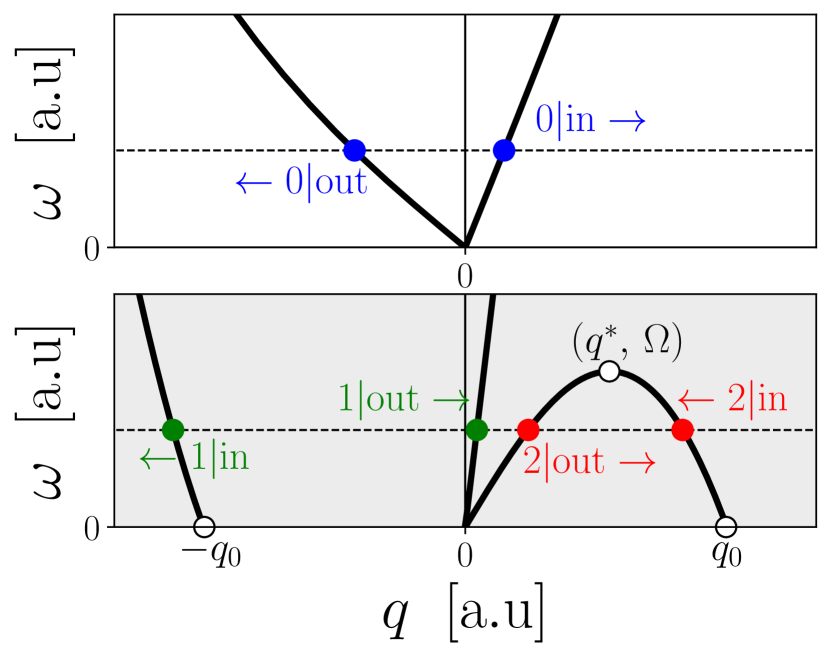
Figure 1: Graphical representation of the positive frequency part of the dispersion relation (3) in the far upstream subsonic (upper plot) and downstream supersonic (lower plot) regions. The background color of the lower plot is greyed for recalling that it concerns the interior of the analogue black hole. In both plots the horizontal dashed line represents the angular frequency $\omega$ of a given excitation. In the upstream region there are two channels of propagation associated to each value of $\omega$. In the downstream region there are four (two) propagation channels when $\omega$ is smaller (larger) than the threshold $\Omega$ defined in Eq. (7). The channels are denoted as 0, 1 or 2, with an additional “in” (“out”) label indicating if the wave propagates towards (away from) the horizon. The direction of propagation of each channel is marked with an arrow.

From the identification of the relevant channels and of their direction of propagation it is possible to define quantum modes forming a basis enabling to describe all the elementary excitations of the background flow. To each such mode is associated a quantum operator: $\hat{b}_{i}^{\dagger}(\omega)$ and $\hat{b}_{i}(\omega)$ ($i=0$, 1 or 2) are the creation and annihilation operators of an excitation of energy $\hbar\omega$ which is ingoing in channel $i|{\rm in}$ and scattered by the horizon onto the three outgoing channels $0|{\rm out}$, $1|{\rm out}$ and $2|{\rm out}$. Since each $\hat{b}$ mode is associated with a single ingoing channel, it is denoted as an “ingoing mode”. It is also relevant to define “outgoing modes” associated with a single outgoing channel. The corresponding operators are denoted as $\hat{c}_{i}(\omega)$ and $\hat{c}_{i}^{\dagger}(\omega)$. For instance $\hat{c}^{\dagger}_{0}$ is the creation operator of an excitation where the three ingoing channels are implied and form an outgoing excitation in channel $0|{\rm out}$. The corresponding quantum mode is the analogous Hawking mode. The outgoing modes are related to the incoming ones via the scattering matrix $S(\omega)$:

$$\begin{pmatrix}\hat{c}_{0}\\ \hat{c}_{1}\\ \hat{c}_{2}^{\dagger}\\ \end{pmatrix}=\begin{pmatrix}S_{00}&S_{01}&S_{02}\\ S_{10}&S_{11}&S_{12}\\ S_{20}&S_{21}&S_{22}\\ \end{pmatrix}\,\begin{pmatrix}\hat{b}_{0}\\ \hat{b}_{1}\\ \hat{b}_{2}^{\dagger}\\ \end{pmatrix},$$ (5)

where all the $\omega$ dependencies have been omitted for legibility. The modes $\hat{b}_{2}$ and $\hat{c}_{2}$ are particular in the sense that they have a negative norm and should be quantized inverting the usual role of the creation and annihilation operators [33] in order to satisfy the standard Bose commutation relations. The mode $\hat{c}_{2}$ is analogous to what is called the partner is the context of Hawking radiation. We denote the mode associated with $\hat{c}_{1}$ the companion; Lorentz invariance prevents such a mode to exist in a gravitational black hole, but it is unavoidable in an analog system.

The fact that the outgoing operators fulfil the canonical commutation relations implies that the scattering matrix $S(\omega)$ obeys the skew-unitarity condition

$$S^{\dagger}\eta S=\eta=S\eta S^{\dagger},\quad\mbox{where}\quad\eta={\rm diag}(1,1,-1)\;.$$ (6)

For $\omega>\Omega$ the mode with subscript 2 (the partner) disappears because the corresponding ingoing and outgoing channels do (cf. Fig. 1) and the $S$-matrix becomes $2\times 2$ and unitary. In this case the vacuum of the outgoing modes (the $\hat{c}$’s) is identical to the vacuum of the incoming ones (the $\hat{b}$’s) and the analogous Hawking effect disappears. The value of the corresponding threshold energy is

$$\begin{split}&\Omega=q^{*}V_{d}-\omega_{{\scriptscriptstyle\rm B},d}(q^{*})\quad\mbox{with}\\ &q^{*}\xi_{d}=\left(-2+\frac{m_{d}^{2}}{2}+\frac{m_{d}}{2}\sqrt{8+m_{d}^{2}}\right)^{\frac{1}{2}}.\end{split}$$ (7)

It has been shown in Ref. [20] that the three-mode system describing the analogous black hole horizon can be modeled by an optical setup simply composed of a parametric amplifier and a beam splitter, as depicted in Fig. 2.

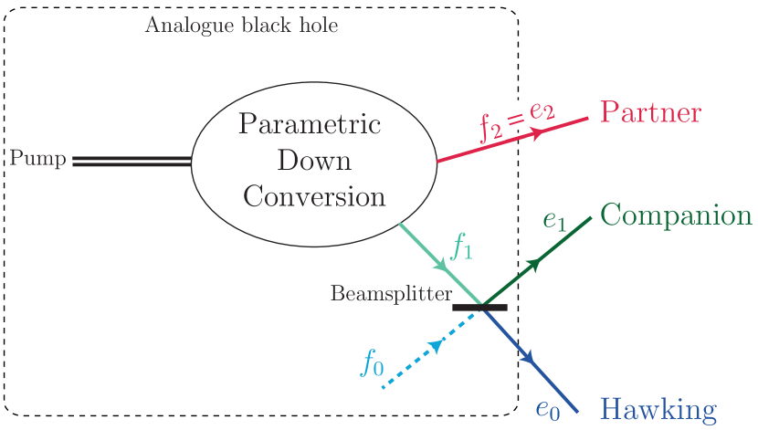
Figure 2: Model optical system equivalent to the analogous black hole. The explicit relationship of the effective modes $f_{i}$ and $e_{i}$ ($i=0,1$ and 2) with the physical outgoing modes is given in Eqs. (51) and (52). The $f_{0}$ mode is represented with a dashed line because, contrarily to modes $f_{1}$ and $f_{2}$, it is not occupied at zero temperature, see Eqs. (56). The long wavelength transmission coefficient of the beam splitter is denoted as $\Gamma_{0}$ in Appendix B. It plays the role of the grey body factor of the analogous black hole.

Entanglement is localized in the two-mode squeezed state $f_{1}|f_{2}$. It is then dispatched by mean of a beam splitter which performs a non local transformation from the effective modes $(f_{0},f_{1},f_{2})$ onto other effective modes $(e_{0},e_{1},e_{2})$ which connect to the physical outgoing modes $(c_{0},c_{1},c_{2})$ by a simple local linear unitary Bogoliubov transformation (LLUBO), see details in Appendix C. We stress that the configuration depicted in Fig. 2 captures the essence of the analogue black hole configuration and is generic: A similar model has been used in Ref. [34] for describing an optical system containing a pair white-black hole analog and then studied on general grounds in [35]. Albeit the fact that we allow the down-conversion process to violate Lorentz invariance (since we enforce the Bogoliubov dispersion relation) the two-mode squeezed state built on $\hat{f}_{1}$ and $\hat{f}_{2}$ is the closest possible analogue to an ideal black hole. The additional beam splitter is inherent to any analogue model. The transmission coefficient of this beam splitter plays the role of the grey-body factor which is relevant in the gravitational context, see discussion in [20].

II.2 Density matrix and measure of bipartite entanglement

For describing analog black holes physics one should consider observables operating in the Fock space of the outgoing modes, as would an observer located outside the horizon of a gravitational black hole. However, the physical implementation of the analog black hole configurations presented in Appendix A is realized in the vacuum of the incoming modes. This mismatch is the origin of the quantum evaporation process, as first presented by Hawking [4]. An ingoing vacuum mode of frequency $\omega$ (which we denote as $|0_{\omega}\rangle^{\rm in}$) relates to an outgoing vacuum mode $|0_{\omega}\rangle^{\rm out}$ through

$$|0_{\omega}\rangle^{\rm in}=\frac{1}{|S_{22}|}\,e^{\left(X_{02}\,\hat{c}_{0}^{\dagger}+X_{12}\,\hat{c}_{1}^{\dagger}\right)\,\hat{c}_{2}^{\dagger}}\,|0_{\omega}\rangle^{\rm out},$$ (8)

where the coefficients $X_{i2}$ ($i=0$ and 1) are expressed in terms of entries of the $S$-matrix (5): $X_{i2}(\omega)=S_{i2}(\omega)/S_{22}(\omega)$, and

$$|0_{\omega}\rangle^{\rm out}=|0_{\omega}\rangle_{0}^{\rm out}\otimes|0_{\omega}\rangle_{1}^{\rm out}\otimes|0_{\omega}\rangle_{2}^{\rm out},$$ (9)

where $|0_{\omega}\rangle_{j}^{\rm out}$ is the vacuum of operator $\hat{c}_{j}(\omega)$, with $j\in\{0,1,2\}$. Eq. (8) can be rewritten in terms of the number states of quasi-particles of type $c_{j}$

$$|n_{\omega}\rangle_{j}=\frac{1}{\sqrt{n!}}\left(\hat{c}_{j}^{\dagger}(\omega)\right)^{n}|0_{\omega}\rangle_{j}^{\rm out},$$ (10)

as

$$|0\rangle^{\rm in}=\frac{1}{|S_{22}|}\sum_{\mu,\nu=0}^{\infty}\sqrt{\binom{\mu+\nu}{\mu}}X_{\scriptscriptstyle 02}^{\mu}X_{\scriptscriptstyle 12}^{\nu}|\mu\rangle_{\scriptscriptstyle 0}|\nu\rangle_{\scriptscriptstyle 1}|\mu+\nu\rangle_{\scriptscriptstyle 2}.$$ (11)

It will be often the case below that, as in expression (11), we drop the explicit $\omega$-dependence for legibility.

Relationships (8) and (11) ensure that the system is in a pure three modes Gaussian state which is fully characterized by its $6\times 6$ covariance matrix $\sigma(\omega)$ with entries

$$\sigma_{\ell m}\equiv\frac{1}{2}\,\langle\hat{\xi}_{\ell}\,\hat{\xi}_{m}+\hat{\xi}_{m}\,\hat{\xi}_{\ell}\rangle-\langle\hat{\xi}_{\ell}\rangle\,\langle\hat{\xi}_{m}\rangle,$$ (12)

where operator $\hat{\xi}_{\ell}$ (or $\hat{\xi}_{m}$) is one of the 6 components of the column vector $\hat{\boldsymbol{\xi}}=\sqrt{2}\,(\hat{q}_{0},\hat{p}_{0},\hat{q}_{1},\hat{p}_{1},\hat{q}_{2},\hat{p}_{2})^{\rm\scriptscriptstyle T}$, where

$$\hat{q}_{j}(\omega)=\frac{1}{\sqrt{2}}(\hat{c}_{j}+\hat{c}_{j}^{\dagger})\quad\mbox{and}\quad\hat{p}_{j}(\omega)=\frac{i}{\sqrt{2}}(\hat{c}_{j}^{\dagger}-\hat{c}_{j}).$$ (13)

In expression (12) and in all the following, the averages $\langle\cdots\rangle$ are performed over the density matrix of the system. This density matrix is simply $\rho=|0\rangle^{\rm in}\,{}^{\rm in}\langle 0|$ in the ideal case just described. We also consider more realistic situations where some incoherent excitations are present and the system is not in a pure state. A simple manner to account for this situation would be to assume that the system is in a thermal state. This is however impossible because the analog configurations depicted in Appendix A are thermodynamically unstable. A way to circumvent this problem has been proposed in Refs. [36, 37]. It consists in postulating that the system was initially in thermal equilibrium at temperature $T$ with a constant density and velocity ($n_{u}$ and $V_{u}$, respectively) and that the flow has been adiabatically modified by slowly ramping the appropriate external potential, eventually reaching the black hole configuration of interest. This situation, although idealized, it less schematic than the zero excitation regime. It emulates the experimental situation of Refs. [18, 19] if the system is considered to have been initially in equilibrium in the frame attached to the flowing condensate. In this case one has (for $j\in\{0,1,2\}$)

$$\bar{n}_{j}(\omega)\equiv\langle\hat{b}^{\dagger}_{j}(\omega)\hat{b}_{j}(\omega)\rangle=n_{\rm\scriptscriptstyle th}\!\left[\omega_{{\scriptscriptstyle\rm B},\alpha}\!\left(q_{j|\rm in}(\omega)\right)\right],$$ (14)

where $n_{\rm\scriptscriptstyle th}(\omega)$ is the thermal Bose occupation distribution at temperature $T$ and energy $\hbar\omega$, whereas $\omega_{{\scriptscriptstyle\rm B},\alpha}(q_{j|\rm in})$ is the Bogoliubov dispersion relation (4), with $\alpha=u$ if $j=0$ and $\alpha=d$ if $j=1$ or 2. The functions $q_{j|\rm in}(\omega)$ appearing in expression (14) are pictorially defined in Fig. 1. For instance $q_{2|\rm in}(\omega)$ is the function that, to a given angular frequency $\omega\in[0,\Omega]$, associates a wave-vector along the $2|\rm in$ dispersion branch. We loosely refer to the cases where $\bar{n}_{j}$ ($j\in\{0,1,2\}$) is equal to the right-hand side (r.h.s.) of (14) as “finite temperature” situations. In the simplest configuration, denoted as “zero temperature” the system is in the pure state $|0\rangle^{\rm in}$ and the $\bar{n}_{j}$’s are all equal to zero. We will not specify the values of the $\bar{n}_{j}$’s in the following, so that the formulas we give are generally valid, even in situations where the occupation numbers should not be given by formulas of the type of Eq. (14). However, for illustrative purposes, all the figures of the paper are plotted in specific temperature cases.

Several observables have been proposed to theoretically evaluate the bipartite entanglement in the context of analogue gravity, such as the Cauchy-Schwarz criterion [38, 39, 40, 41, 42, 43], the generalized Peres-Horodecki parameter [44, 45], the logarithmic negativity [46, 47, 48, 49], the entanglement entropy [50, 49], the entanglement of formation [51], the Gaussian contangle [20]. In the present work, for reasons exposed in Appendix B, we chose to evaluate the bipartite entanglement between modes $i$ and $j$ by means of a quantity $\Lambda^{(i|j)}(\omega)\in]-\infty,1]$ which is a monotonous measure of entanglement that has been denoted as the “PPT measure” in Ref. [20]. States $i$ and $j$ are separable when $\Lambda^{(i|j)}<0$, which is always the case when $(i|j)=(0|1)$: the companion and the Hawking modes are not entangled. The two other couples of modes, $(0|2)$ and $(1|2)$, are always entangled at $T=0$ for all $\omega$. Their entanglement decreases with increasing temperature by an amount specified by the PPT measure which reads explicitly ($i=0$ or 1) [20]:

$$\begin{split}\Lambda^{(i|2)}(\omega)=&-\langle\hat{c}_{i}^{\dagger}\,\hat{c}_{i}\rangle-\langle\hat{c}_{2}^{\dagger}\,\hat{c}_{2}\rangle\\ &+\sqrt{\left(\langle\hat{c}_{i}^{\dagger}\,\hat{c}_{i}\rangle-\langle\hat{c}_{2}^{\dagger}\,\hat{c}_{2}\rangle\right)^{2}+4|\langle\hat{c}_{i}\,\hat{c}_{2}\rangle|^{2}}\;.\end{split}$$ (15)

As clear from the above expression, a key ingredient for characterizing entanglement is the determination of average values of different combination of two creation or annihilation operators of the outgoing modes. At the experimental level, this determination could reveal difficult for quantities such as $\langle\hat{c}_{0}\,\hat{c}_{2}\rangle$ for instance. Steinhauer proposed a possible way to extract this information from the knowledge of the density-density correlation function [42]. As stressed in Refs. [52, 53] this method needs to be used with more care than initially thought, but is indeed a possible manner to obtain the information. At the theoretical level, it is a straightforward matter to compute the expectation values of products of the ingoing creation and annihilation operator (quantities such as (14) for instance). From there, expression (5) makes it possible to compute the equivalent expressions for the outgoing operators, which are the quantities of interest. The relevant formulae are given in Appendix B, Eqs. (46).

III Bipartite nonlocality

Most Bell-like inequalities proposed in the context of continuous variables hinge on a discretization process [54, 55, 56, 57, 58, 59]. Indeed, since the set of outcomes for a given observable is typically unbounded in continuous variable systems, it seems a priori difficult to derive an upper bound of the expectation value of a Bell-type observable. It is not impossible, though: relying on the Fine–Abramsky–Brandenburger theorem [60, 61], the authors of Refs. [62, 63] were able to derive continuous Bell inequalities for continuous and unbounded observables. However, to our knowledge, no practical (theoretical or experimental) use of such fully continuous approaches has been successfully implement so far. A method to circumvent this difficulty is based on discretization and consists of using a dichotomic binning of the outcome results. In this case, by using observables which rely on continuous measurements but can only take a finite number of outcomes, one can construct a Bell inequality similar to those derived for discrete variables. A well-known example of such observables are the so-called pseudo-spin operators: they live in an infinite-dimensional Hilbert space but the outcome of their measurement is either $-1$ or $+1$.

Due to its practicability, we chose to follow this discretization approach to derive Bell-like inequalities in the context of BEC analogue black holes. In this work we use the GKMR (Gour, Khanna, Mann and Revzen) pseudo-spins introduced in Ref. [64]: To an outgoing mode $j$ ($j\in\{0,1,2\}$) of energy $\omega$ is associated a Hermitian vectorial operator $\hat{\boldsymbol{\Pi}}{}^{(j)}(\omega)$ with Cartesian coordinates

$$\hat{\Pi}^{(j)}_{x}(\omega)=\int_{0}^{+\infty}{\rm d}q\,\Big{(}|q\rangle_{j}\,{}_{j}\!\langle q|-|-q\rangle_{j}\,{}_{j}\langle-q|\Big{)},$$ (16a)

$$\hat{\Pi}^{(j)}_{y}(\omega)=i\int_{0}^{+\infty}{\rm d}q\,\Big{(}|q\rangle_{j}\,{}_{j}\langle-q|-|-q\rangle_{j}\,{}_{j}\langle q|\Big{)},$$ (16b)

$$\hat{\Pi}^{(j)}_{z}(\omega)=\int_{-\infty}^{+\infty}{\rm d}q\,|q\rangle_{j}\,{}_{j}\langle-q|,$$ (16c)

where $|q\rangle_{j}$ is the eigenstate associated to the eigenvalue $q$ of the position operator $\hat{q}_{j}(\omega)$ (13). The operators (16) anti-commute with each others and all square to unity. They verify the expected spin commutation relations, such as

$$\left[\hat{\Pi}_{x}^{(j)},\hat{\Pi}_{y}^{(j)}\right]=2\,i\,\hat{\Pi}_{z}^{(j)},$$ (17)

and similar relations upon circular permutations of the indices $x$, $y$ and $z$. In Appendix D we recall the properties of the pseudo-spin operator and of its eigenvalues which are useful in the following.

These pseudo-spin operators have been studied in contexts similar to ours in Refs. [59, 65, 66]. Compared with other pseudo-spin operators such as for instance those introduced by Banaszek and Wodkiewicz [67, 68], the GKMR spins (16) have the advantage of having simple Wigner transforms, which makes the computation of their expectation values over Gaussian states relatively easy, as detailed in Appendix E. We stress here that different choices of spin representation lead to different values of averages of the Bell operators (18) [64]. From this remark naturally results that, generally speaking, the observables (19), (21) and (32) we use below are witnesses of nonlocality: Their violation of Bell-type inequalities is a sufficient but not necessary test of nonlocal behavior. As a final remark, we note here an unforeseen benefit of the use of the pseudo-spin operators (16): it will be shown in Sec. IV that the structure of the zero temperature ground state of the analog system (the vacuum $|0\rangle^{\rm in}$) is most easily analyzed in terms of a combination of eigenstates of operator $\hat{\Pi}_{x}$.

Equipped with the pseudo-spin operators (16) we can define a CHSH Bell operator [69] measuring the correlations between the emitted quasi-particles of type $i$ and $j$:

$$\begin{split}\hat{\mathscr{B}}{}^{(i|j)}(\omega)=&(\boldsymbol{a}+\boldsymbol{a}^{\prime})\cdot\hat{\boldsymbol{\Pi}}{}^{(i)}\otimes\boldsymbol{b}\cdot\hat{\boldsymbol{\Pi}}{}^{(j)}\\ +&(\boldsymbol{a}-\boldsymbol{a}^{\prime})\cdot\hat{\boldsymbol{\Pi}}{}^{(i)}\otimes\boldsymbol{b}^{\prime}\cdot\hat{\boldsymbol{\Pi}}{}^{(j)},\end{split}$$ (18)

where $\boldsymbol{a}$, $\boldsymbol{a}^{\prime}$, $\boldsymbol{b}$ and $\boldsymbol{b}^{\prime}$ are unit vectors. Given a unit vector $\boldsymbol{n}$ it is easily checked that $(\boldsymbol{n}\cdot\hat{\boldsymbol{\Pi}}{}^{(j)})^{2}=\mathbb{1}$, meaning that the Hermitian operator $\boldsymbol{n}\cdot\hat{\boldsymbol{\Pi}}{}^{(j)}$ has eigenvalues $\pm 1$. It then follows from direct inspection that, if one believes in local realism, one should expect that a measure of the operator $\hat{\mathscr{B}}{}^{(i|j)}$ yields a result $\pm 2$ [70]. The tenant of local realism is thus violated when $\langle\hat{\mathscr{B}}{}^{(i|j)}\rangle>2$, whereas Cirel’son bound [71] imposes $\langle\hat{\mathscr{B}}{}^{(i|j)}\rangle\leq 2\sqrt{2}$. Since the modes 0 and 1 are not entangled the quantity $\langle\hat{\mathscr{B}}{}^{(0|1)}\rangle$ is always lower than 2 and its computation is of no interest to us. For attempting to violate as much as possible Bell inequality one should consider the modes 0 and 2 (or 1 and 2) and look for an arrangement of the four measurement directions $\boldsymbol{a}$, $\boldsymbol{a}^{\prime}$, $\boldsymbol{b}$ and $\boldsymbol{b}^{\prime}$ which maximizes $\langle\hat{\mathscr{B}}{}^{(i|2)}\rangle$ ($i=0$ or 1). This procedure is explained in Appendix F and makes it possible to analytically compute the quantity

$$B^{(i|2)}(\omega)\equiv\,\mbox{max}_{\boldsymbol{a},\boldsymbol{a}^{\prime},\boldsymbol{b},\boldsymbol{b}^{\prime}}\left\langle\hat{\mathscr{B}}{}^{(i|2)}(\omega)\right\rangle.$$ (19)

The corresponding explicit expression is given in Eq. (101b).

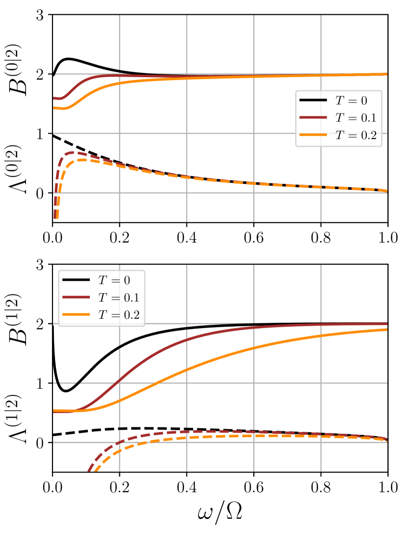
Figure 3: Plot of $B^{(i|2)}$ (solid lines) and $\Lambda^{(i|2)}$ (dashed lines) as functions of $\omega$ for the waterfall configuration with $m_{d}=2.9$ and different temperatures. We only consider the range of frequencies $\omega<\Omega$ for which the vacuum of the outgoing and ingoing modes do not coincide. The value of the temperature is indicated in units of $g\,n_{u}=mc_{u}^{2}$. Upper plot: $i=0$, lower plot $i=1$. Non separability of modes $i$ and $2$ is achieved when $\Lambda^{(i|2)}>0$. Bell inequality is violated when $B^{(i|2)}>2$.

The values of $B^{(0|2)}$ and $B^{(1|2)}$ are plotted as functions of $\omega$ for different temperatures in Fig. 3 for a waterfall configuration with a downstream Mach number $m_{d}\equiv V_{d}/c_{d}=2.9$, the same as in the Technion 2019 experiment [18]. We also plot for comparison the values of the corresponding PPT measures $\Lambda^{(0|2)}$ and $\Lambda^{(1|2)}$, as defined by (15). The figure illustrates that, as well known, entanglement is necessary but not sufficient for violating Bell inequality. Also, the amount by which the Bell inequality is violated is not proportional to the amount of entanglement. This is clearly seen, for instance, by comparing the values of $B^{(0|2)}$ and $\Lambda^{(0|2)}$ at $T=0$: the maximum violation of Bell inequality is not achieved for the maximal entanglement. One can also notice that the violation of Bell inequality is much less resilient to temperature than is the entanglement. These features can be most easily understood in the framework of the optical model represented in Fig. 2. They originate from the the dilution of entanglement between the three modes caused by the beam splitter, as discussed in Appendix C.

Fig. 3 indicates that, in the waterfall configuration we consider (with $m_{d}=2.9$), the entanglement is lower and the violation of Bell inequality less significant for the correlations among modes 1 and 2 than for the correlations among modes 0 and 2. However, this is not always the case. This point is illustrated in Fig. 4 which displays, for all waterfall configurations, the zero temperature values of ${\rm max}_{\omega}B^{(i|2)}$ and ${\rm max}_{\omega}\Lambda^{(i|2)}$ (for $i=0$ and 1) as functions of the upper Mach number $m_{u}$ (the maximisation is performed at fixed $m_{u}$, for $\omega\in[0,\Omega]$). All the possible waterfall configurations are considered since $m_{u}$ spans the whole interval $[0,1]$. In this figure we aim at evaluating the largest amount of entanglement and nonlocality reached in each configuration. This is the reason why we plot the maximum values taken by the quantities $\Lambda^{(i|2)}$ and $B^{(i|2)}$ over the energy interval $[0,\Omega]$ [where $\Omega$ is defined by Relation (7)] since this is only for energies in this interval that spontaneous emission of quasi-particles occurs.

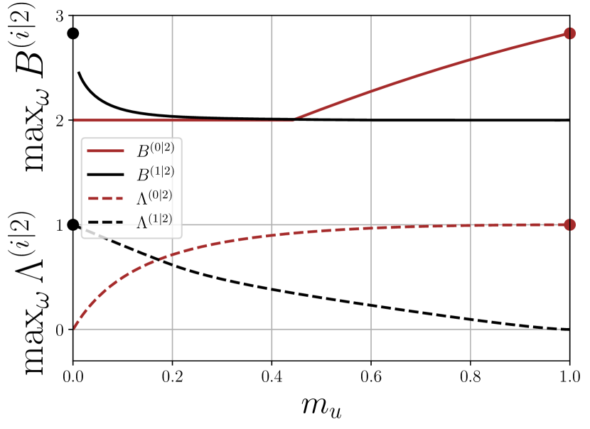
Figure 4: Zero temperature value of the CHSH parameter and of the PPT measure characterizing non separability of modes $i$ ($=0$ and 1) and 2 for the waterfall configuration. The maximal value reached by these quantities over the interval $\omega\in[0,\Omega]$ is plotted as a function of the upper Mach number $m_{u}$ which (as explained in Appendix A) characterizes a given configuration. The values of $B^{(1|2)}$ for $m_{u}\leq 0.01$ are not indicated because of lack of numerical precision. The upper bounds of $B^{(i|2)}$ and $\Lambda^{(i|2)}$ ($\sqrt{8}$ and 1, respectively) are indicated with filled dots.

For instance, the situation depicted in Fig. 3 ($m_{d}=2.9$) corresponds in Fig. 4 to the point $m_{u}=0.587$ since for waterfall configurations $m_{u}$ and $m_{d}$ are related by (37a). And indeed, Fig. 4 shows that for this value of $m_{u}$ the maximum over $\omega$ of $B^{(0|2)}$ is 2.25, and the one of $B^{(1|2)}$ is 2, as observed in Fig. 3.

Fig. 4 shows that for values of $m_{u}$ larger than 0.6, the entanglement is mainly concentrated between modes 2 and 0, i.e., between the Hawking quantum and the partner. This is indicated by the fact that both the PPT measure and the CHSH parameter significantly point to nonseparability and nonlocality between these two modes. For $m_{u}\leq 0.2$ instead, the figure shows that entanglement is concentrated between the partner and the companion (modes 2 and 1, respectively).

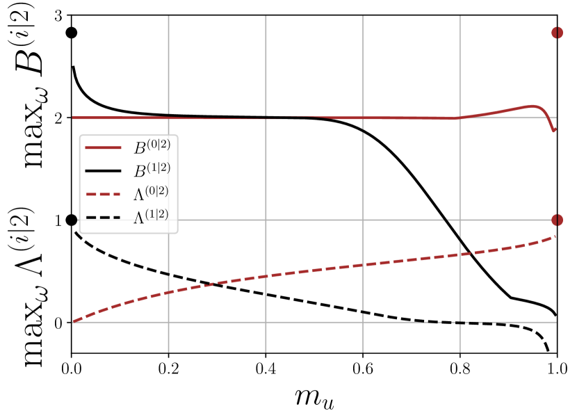
Figure 5: Same as Fig. 4 for a temperature $T=0.2\,gn_{u}$. Contrarily to what is observed in the zero temperature case displayed in Fig. 4, the maxima of $\Lambda$ and $B$ (1 and $2\sqrt{2}$, respectively) are never reached.

A plot similar to the one of Fig. 4, but where the quantities are evaluated at finite temperature, enables to evaluate the resilience of entanglement and non-separability to an increase of temperature. This check is performed in Fig. 5 which shows that, whereas at $T=0.2\,gn_{u}$ the PPT measure is not dramatically affected, the CHSH parameters $B^{(0|2)}$ and $B^{(1|2)}$ no longer show evidences of violation of Bell inequality, except in the $(1|2)$ sector for waterfall configurations with $m_{u}\lesssim 0.15$ and, in a lesser extent, in the $(0|2)$ sector for $m_{u}\gtrsim 0.85$.

Figs. 4 and 5 illustrate a specific feature of analog models: there is no recipe enabling to qualify one of the positive norm modes (in our specific case, mode 0 or 1) as unessential. For instance, it is incorrect to study the system discarding a priori the companion (mode 1) from one’s analysis. Fig. 4 shows that, at zero temperature, this is allowed in some regions of parameters, but incorrect in others. Fig. 5 even shows that only the companion-partner correlations display violation of Bell inequality above a certain temperature. In this instance it is the Hawking mode which is unessential. It is therefore important to give a proper account of all the modes involved in our analog system.

Another way to consider the same problem is to use the equivalent model depicted in Fig. 2: it is well known that a nondegenerate optical parametric amplifier generates an EPR state when the squeezing parameter tends to infinity (see, e.g., Ref. [73]). As discussed in Appendix C this is the case for the two mode squeezed state (55) when $\omega\to 0$. The zero energy transmission coefficient $\Gamma_{0}$ of the effective beam splitter (pictorially defined in Fig. 2) tends to 0 or 1 when the upper Mach number $m_{u}$ tends to 0 or 1, respectively [see e.g., Eq. (49) which holds for the waterfall configuration]. In these two limits the system forms an EPR state between two of the three outgoing modes (and the third one can be omitted). This EPR state involves, either the Hawking quantum and the partner (when $m_{u}\to 1$) or the companion and the partner (when $m_{u}\to 0)$. This is the reason why the entanglement and nonlocality bounds are reached in this two limits in Fig. 4, and similarly in Figs. 11 and 12 of Appendix I for the delta peak and flat profile configurations, respectively.

We conclude this section by noticing that, from a quantum information perspective, the fact that reduced bipartite states of a tripartite system are entangled is of no particular significance per se. It is however important for future experimental studies of analog systems to determine for which configurations, and to quantify to which extent, the three-mode acoustic Hawking emission is bipartite entangled and nonlocal. Besides, we will see in the next section that this resilience of entanglement to partial tracing acquires a particular significance when examining the exact nature of the long wavelength components of the three-mode state $|0\rangle^{\rm in}$ (the ground state of the system).

IV tripartite nonlocality

Equipped with the same pseudo-spin operators as the ones defined in Sec. III one can define a three-mode Bell operator of a type similar to the two-mode one (18). This operator measures the correlations between the outgoing quasi-particles of type $i$, $j$ and $k$. It is defined as [74, 75]:

$$\hat{\mathscr{S}}{}^{(i|j|k)}(\omega)=\tfrac{1}{2}\hat{\mathscr{B}}{}^{(i|j)}\otimes\boldsymbol{c}^{\prime}\cdot\hat{\boldsymbol{\Pi}}{}^{(k)}+\tfrac{1}{2}\hat{\mathscr{B}}^{\prime}{}^{(i|j)}\otimes\boldsymbol{c}\cdot\hat{\boldsymbol{\Pi}}{}^{(k)},$$ (20)

where $\hat{\mathscr{B}}^{\prime}{}^{(j|k)}(\omega)$ is the same as $\hat{\mathscr{B}}{}^{(j|k)}(\omega)$ defined in (18) with the primes reversed, and $\boldsymbol{c}$ and $\boldsymbol{c}^{\prime}$ are normalized vectors (as well as $\boldsymbol{a}$, $\boldsymbol{a}^{\prime}$, $\boldsymbol{b}$, and $\boldsymbol{b}^{\prime}$ involved in the definition of $\hat{\mathscr{B}}{}^{(j|k)}$). Expanding expression (20) shows that $\hat{\mathscr{S}}{}^{(i|j|k)}$ is invariant upon a permutation of its indices, provided the names of the unit vectors $(\boldsymbol{a},\boldsymbol{b},\boldsymbol{c})$ and $(\boldsymbol{a}^{\prime},\boldsymbol{b}^{\prime},\boldsymbol{c}^{\prime})$ undergo the same permutation. In the following we arbitrarily chose the order $(i,j,k)=(0,1,2)$.

Similarly to what occurs for the two-mode operator, the principle of local realism, if correct, should predict that a measure of the operator $\hat{\mathscr{S}}{}^{(0|1|2)}$ yields results $\pm 2$. The system violates this principle when the average of the operator (20) is larger than two. This is often referred to as violation of Svetlichny inequality. It is important to note that the observable $\hat{\mathscr{S}}{}^{(0|1|2)}$ is specially designed in order to be sensitive to genuine tripartite nonlocality (see discussions in Refs. [74, 76, 75, 21] and references therein): a tripartite system can involve nonlocal correlations between any of its bipartitions and still not violate the Svetlichny inequality $\langle\hat{\mathscr{S}}{}^{(0|1|2)}\rangle<2$. A simple example of a system which displays two mode nonlocality but does not pass the Svetlichny test is presented in Appendix C [see Eq. (64) and the discussion below].

For attempting to reach a maximum violation of Svetlichny (i.e., three-mode Bell) inequality it is necessary to choose a particular arrangement of the vectors $\boldsymbol{a}$, $\boldsymbol{a}^{\prime}$, $\boldsymbol{b}$, $\boldsymbol{b}^{\prime}$, $\boldsymbol{c}$ and $\boldsymbol{c}^{\prime}$ which maximizes the expectation value $\langle\hat{\mathscr{S}}{}^{(0|1|2)}\rangle$. Do do so, we resort to a genetic algorithm which is presented in Appendix G and numerically determines the quantity

$$S^{(0|1|2)}(\omega)\equiv\,\mbox{max}_{\boldsymbol{a},\boldsymbol{a}^{\prime},\boldsymbol{b},\boldsymbol{b}^{\prime},\boldsymbol{c},\boldsymbol{c}^{\prime}}\left\langle\hat{\mathscr{S}}{}^{(0|1|2)}(\omega)\right\rangle.$$ (21)

It is shown in Appendix H that the tripartite parameter $S^{(0|1|2)}(\omega)$ is bounded from above by $2\sqrt{2}$ [this is Eq. (108)] and that this bound is reached at $\omega=0$ and $T=0$ [see Eq. (118)]. The behavior of $S^{(0|1|2)}(\omega)$ at zero temperature is displayed in Fig. 6 for different realizations of the waterfall configuration. Although the bound $2\sqrt{2}$ is reached in the long wave length limit for all the configurations, even a weak temperature is able to destroy the signal of nonlocality as illustrated in Fig. 7.

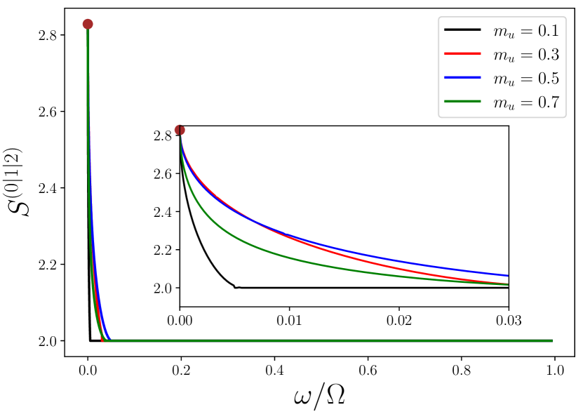
Figure 6: Zero temperature value of the tripartite parameter $S^{(0|1|2)}$ plotted as a function of energy for different realization of the waterfall configuration, each being characterized by the upstream Mach number $m_{u}$. The inset displays a blow up of the figure at low energy. The upper bound $2\sqrt{2}$ is marked by a brown dot. It is reached at $\omega=0$ in all configurations.

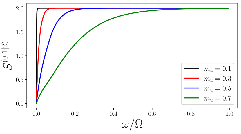
Figure 7: Same as Fig. 6 for a temperature $T=0.05\,gn_{u}$. At variance with the zero temperature situation the tripartite measure (21) is here always lower or equal to 2.

This is connected to the loss of purity of the finite temperature system and can be understood analytically, again in the long wave length limit, as discussed in Appendix G. This sensitivity to a small finite temperature probably precludes the experimental observation of tripartite nonlocality by means of the observable (21). However, although the zero temperature behavior is certainly difficult to observe, it is rich of fundamental insight on the nature of the state of the system, as we now discuss.

As argued in Appendix E, the fact that, at zero temperature and $\omega=0$ the system reaches the tripartite upper bound ($S^{(0|1|2)}=2\sqrt{2}$, see Fig. 6) mathematically stems from the fact that, under these conditions the system is in a pure state and displays perfect correlations in the following expectation values [see Eqs. (91), (92) and (82)]:

$$\begin{split}\langle\hat{\Pi}_{y}^{(0)}\otimes\hat{\Pi}_{y}^{(1)}\otimes\hat{\Pi}_{z}^{(2)}\rangle&=\langle\hat{\Pi}_{y}^{(0)}\otimes\hat{\Pi}_{z}^{(1)}\otimes\hat{\Pi}_{y}^{(2)}\rangle\\ &=-\langle\hat{\Pi}_{z}^{(0)}\otimes\hat{\Pi}_{y}^{(1)}\otimes\hat{\Pi}_{y}^{(2)}\rangle\\ &=\langle\hat{\Pi}_{z}^{(0)}\otimes\hat{\Pi}_{z}^{(1)}\otimes\hat{\Pi}_{z}^{(2)}\rangle=1.\end{split}$$ (22)

All the other expectation values of products of three components of the $\hat{\boldsymbol{\Pi}}$ operator are zero. Since all the operators in (22) have only $\pm 1$ as eigenvalues, this means that each term must reach its extremal value and the vacuum mode of zero frequency $|0_{\omega=0}\rangle^{\rm in}$ must therefore be an eigenstate of the operators appearing in (22):

$$\hat{\Pi}_{y}^{(0)}\otimes\hat{\Pi}_{y}^{(1)}\otimes\hat{\Pi}_{z}^{(2)}|0_{\omega=0}\rangle^{\rm in}=+|0_{\omega=0}\rangle^{\rm in},$$ (23a)

$$\hat{\Pi}_{y}^{(0)}\otimes\hat{\Pi}_{z}^{(1)}\otimes\hat{\Pi}_{y}^{(2)}|0_{\omega=0}\rangle^{\rm in}=+|0_{\omega=0}\rangle^{\rm in},$$ (23b)

$$\hat{\Pi}_{z}^{(0)}\otimes\hat{\Pi}_{y}^{(1)}\otimes\hat{\Pi}_{y}^{(2)}|0_{\omega=0}\rangle^{\rm in}=-|0_{\omega=0}\rangle^{\rm in},$$ (23c)

$$\hat{\Pi}_{z}^{(0)}\otimes\hat{\Pi}_{z}^{(1)}\otimes\hat{\Pi}_{z}^{(2)}|0_{\omega=0}\rangle^{\rm in}=+|0_{\omega=0}\rangle^{\rm in}.$$ (23d)

Relations (23) define a state which exhibits the GHZ paradox, contradicting local hidden variable theories by means of a single measurement; cf. e.g., the discussion in [77]. In the same line, the above noted fact that our system saturates the upper bound $2\sqrt{2}$ of the Svetlichny parameter is a characteristic also shared by GHZ states. Another resemblance lies in the fact that the GHZ states possess maximal tripartite entanglement, quantified by the residual tangle [78, 79] while similarly, in the domain of temperature and energy where Eqs. (23) hold, the residual contangle [80] which measures genuine tripartite entanglement in our continuous variable system diverges [20]. Despite these clear similarities, there is a significant difference between the state $|0_{\omega=0}\rangle^{\rm in}$ and the GHZ states commonly considered in quantum information theory: they have different behaviors upon partial tracing. As well known, taking the partial trace over one of the three modes of a GHZ state yields an unentangled mixed state. At variance, partial tracing the state $|0_{\omega=0}\rangle^{\rm in}$ over modes 0 or 1 leads to an entangled two-mode mixed state, as discussed in Sec. III (see, e.g., the values $\Lambda^{(0|2)}(\omega=0)$ and $\Lambda^{(1|2)}(\omega=0)$ in Fig. 3). As we now argue, the explanation of this conundrum lies in the fact that, whereas the GHZ states are usually build on qubits, the state we consider is an infinite sum of degenerate GHZ states of a continuous variable system.

To tackle this issue it is convenient to expand the state $|0_{\omega=0}\rangle^{\rm in}$ over the eigenstates of the operators $\hat{\Pi}_{x}^{(j)}$ ($j=0$, 1 or 2). As discussed in Appendix D these eigenstates can be written as $|x^{\pm}_{n}\rangle_{j}$: they are labeled by their eigenvalue ($\pm 1$) plus another integer index ($n$ in the above expression) associated to the infinite degeneracy of both eigenvalues. Indeed, at variance with what occurs for a regular spin operator, the projection of the pseudo-spin (16) over a given axis (here $\hat{\Pi}_{x}$) has infinitely degenerate eigenvalues, i.e., there exists an infinite number of mutually orthogonal eigenstates with the same eigenvalue ($+1$ or $-1$):

$$\forall n\in\mathbb{N},\quad\hat{\Pi}_{x}^{(j)}|x^{\pm}_{n}\rangle_{j}=\pm|x^{\pm}_{n}\rangle_{j},$$ (24)

whereas

$$\forall(n,m)\in\mathbb{N}^{2},\quad_{j}\langle x^{\pm}_{n}|x^{\pm}_{m}\rangle_{j}=\delta_{n,m}.$$ (25)

This can be shown by directly constructing the eigenstates of $\hat{\Pi}_{x}$ from the number states, see Eqs. (70) and (71). The expansion of $|0_{\omega=0}\rangle^{\rm in}$ over the complete basis formed by these states is of the form:

$$|0_{\omega=0}\rangle^{\rm in}=\sum_{\begin{subarray}{c}\sigma_{0},\sigma_{1},\sigma_{2}\\ l,m,n\end{subarray}}C^{\sigma_{0},\sigma_{1},\sigma_{2}}_{l,m,n}|x^{\sigma_{0}}_{l},x^{\sigma_{1}}_{m},x^{\sigma_{2}}_{n}\rangle.$$ (26)

In the summation appearing in the above expression, $\sigma_{0}$, $\sigma_{1}$ and $\sigma_{2}=\pm$ whereas $(l,m,n)\in\mathbb{N}^{3}$ and we dropped the indices $j=0$, 1 or 2 of the kets for legibility.

It follows from relations (23) and (73) that:

$$\begin{split}C_{l,m,n}^{-\sigma_{0},-\sigma_{1},-\sigma 2}=-\sigma_{0}\sigma_{1}\,&C_{l,m,n}^{-\sigma_{0},-\sigma_{1},-\sigma_{2}}\\ =-\sigma_{0}\sigma_{2}\,&C_{l,m,n}^{-\sigma_{0},-\sigma_{1},-\sigma_{2}}\\ =\sigma_{1}\sigma_{2}\,&C_{l,m,n}^{-\sigma_{0},-\sigma_{1},-\sigma_{2}}.\end{split}$$ (27)

This imposes that the only nonzero coefficients in expansion (26) are those for which $\sigma_{1}=\sigma_{2}=-\sigma_{0}$. For such coefficients Eqs. (23d) and (73) impose that

$$C^{+--}_{l,m,n}=C^{-++}_{l,m,n}\equiv C_{l,m,n}.$$ (28)

Expansion (26) thus simplifies to

$$\begin{split}|0_{\omega=0}\rangle^{\rm in}=\sum_{l,m,n}C_{l,m,n}\Big{(}&|x^{+}_{l},x^{-}_{m},x^{-}_{n}\rangle\,+\\ &|x^{-}_{l},x^{+}_{m},x^{+}_{n}\rangle\Big{)},\end{split}$$ (29)

which shows that the vacuum $|0_{\omega=0}\rangle^{\rm in}$ of the $\hat{b}_{j}(\omega=0)$ operators (the ingoing ground state) is an infinite sum of degenerate GHZ states. It is this property which enables the reduced state obtained after partial tracing over one mode to remain entangled despite the GHZ nature of the system. Indeed, tracing over mode 0 for instance leads to a reduced density matrix

$$\begin{split}\mbox{Tr}_{(0)}\Big{(}|0_{\omega=0}\rangle^{\rm in}\;{}^{\rm in}\langle 0_{\omega=0}|\Big{)}&=\\ \sum_{m,n,\mu,\nu}{\cal C}^{(0)}_{m,n,\mu,\nu}&\Big{(}|x^{-}_{m}x^{-}_{n}\rangle\,\langle x^{-}_{\mu}x^{-}_{\nu}|\\ &+|x^{+}_{m}x^{+}_{n}\rangle\,\langle x^{+}_{\mu}x^{+}_{\nu}|\Big{)}.\end{split}$$ (30)

In this expression the kets and bras concern modes 1 and 2 (mode 0 has been traced out) and

$${\cal C}^{(0)}_{m,n,\mu,\nu}=\sum_{l=0}^{\infty}C^{*}_{l,\mu,\nu}C_{l,m,n}.$$ (31)

If the eigenvalues $+1$ and $-1$ of operator $\hat{\Pi}_{x}$ were non-degenerate, this would impose $m=\mu$ and $n=\nu$ in expression (30) and the corresponding reduced state would be clearly separable. Nothing similar occurs in our situation, and indeed the reduced states are typically entangled, as shown in Sec. III.

Since we now understand the exact GHZ nature of the zero temperature and $\omega=0$ state of the system, it is of interest to quantify to what extent this feature persists at finite temperature and finite energy. To this aim, we use the genetic algorithm presented in Appendix G to compute the optimum of the Mermin parameter [81, 82]

$$M^{(0|1|2)}(\omega)\equiv\,\mbox{max}_{\boldsymbol{a},\boldsymbol{a}^{\prime},\boldsymbol{b},\boldsymbol{b}^{\prime},\boldsymbol{c},\boldsymbol{c}^{\prime}}\left|\left\langle\hat{\mathscr{M}}{}^{(0|1|2)}(\omega)\right\rangle\right|,$$ (32)

where

$$\begin{split}\hat{\mathscr{M}}^{(0|1|2)}(\omega)=&-\boldsymbol{a}\cdot\hat{\boldsymbol{\Pi}}^{(0)}\otimes\boldsymbol{b}\cdot\hat{\boldsymbol{\Pi}}^{(1)}\otimes\boldsymbol{c}\cdot\hat{\boldsymbol{\Pi}}^{(2)}\\ &+\boldsymbol{a}\cdot\hat{\boldsymbol{\Pi}}^{(0)}\otimes\boldsymbol{b}^{\prime}\cdot\hat{\boldsymbol{\Pi}}^{(1)}\otimes\boldsymbol{c}^{\prime}\cdot\hat{\boldsymbol{\Pi}}^{(2)}\\ &+\boldsymbol{a}^{\prime}\cdot\hat{\boldsymbol{\Pi}}^{(0)}\otimes\boldsymbol{b}\cdot\hat{\boldsymbol{\Pi}}^{(1)}\otimes\boldsymbol{c}^{\prime}\cdot\hat{\boldsymbol{\Pi}}^{(2)}\\ &+\boldsymbol{a}^{\prime}\cdot\hat{\boldsymbol{\Pi}}^{(0)}\otimes\boldsymbol{b}^{\prime}\cdot\hat{\boldsymbol{\Pi}}^{(1)}\otimes\boldsymbol{c}\cdot\hat{\boldsymbol{\Pi}}^{(2)}.\end{split}$$ (33)

We note here that $\hat{\mathscr{S}}^{(0|1|2)}=\tfrac{1}{2}\hat{\mathscr{M}}^{(0|1|2)}+\tfrac{1}{2}\hat{\mathscr{M}}^{\prime}{}^{(0|1|2)}$, where $\hat{\mathscr{M}}^{\prime}{}^{(0|1|2)}$ is the same as $\hat{\mathscr{M}}^{(0|1|2)}$ with the prime reversed [76].

The largest possible value of the Mermin parameter (32) is 4. This upper bound is reached for a state verifying the relations (22), such as a GHZ state or the low wavelength component of the ground state of our system as just discussed. Indeed, at $T=0$, $M^{(0|1|2)}(0)=4$ for all black hole configurations. This is illustrated in Fig. 8

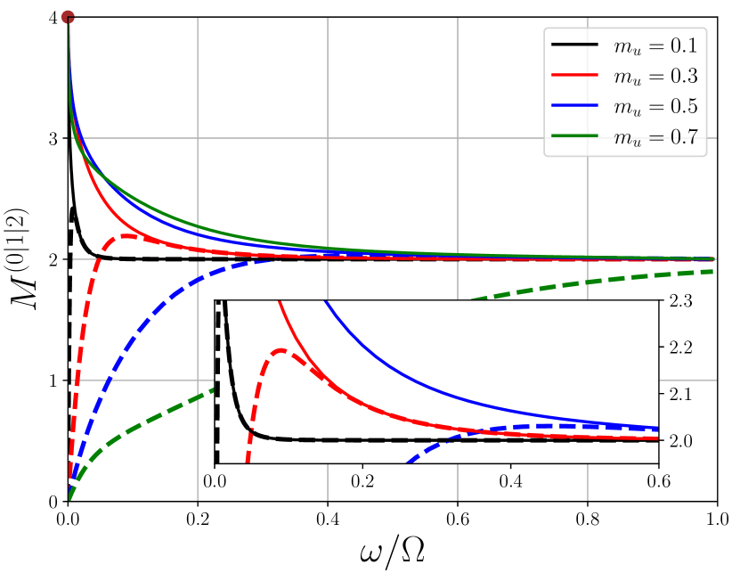
Figure 8: Mermin parameter $M^{(0|1|2)}(\omega)$ plotted for different waterfall configurations. The continuous lines starting from $M^{(0|1|2)}=4$ at $\omega=0$ are zero temperature results and the thick dashed ones (with $M^{(0|1|2)}(0)=0$) correspond to $T=0.1\,gn_{u}$. The inset is a blow up of the figure around the region $M^{(0|1|2)}=2$ for $\omega/\Omega\leq 0.6$.

in which $M^{(0|1|2)}$ is plotted as a function of $\omega$ for different values of $m_{u}$, at zero and finite temperature ($T=0$ and $T=0.1\,gn_{u}$). If the departure of $M^{(0|1|2)}$ from its upper bound is taken as an indication of how much the system differs from a GHZ state, this suggests that the GHZ character of the state is restricted to the low energy and low temperature sector. We stress however that such a criterion is only indicative: The Svetlichny and Mermin parameters provide useful bounds, but not proper measures. This is illustrated by their poor effectiveness for evaluating genuine tripartite entanglement: It is known [76] that if

$$M^{(0|1|2)} >2\sqrt{2},$$ (34a)

$$\mbox{or}\quad S^{(0|1|2)} >2,$$ (34b)

the system exhibits genuine three-mode entanglement. Figs. 6 and 8 show that this type of entanglement is certainly reached at $T=0$ for low energy. However, the criteria (34) are here too restrictive, since the computation of the residual contangle done in Ref. [20] demonstrates that at $T=0$ the system is genuinely tripartite entangled for all energies and all configurations. This general conclusion certainly cannot be reached by inspecting in Figs. 6 and 8 in which domain of energy and for which value of $m_{u}$ the criteria (34) are met. However, these criteria are valid and can be useful, for instance at finite temperature. In this case the state of the system is not pure, the evaluation of the residual contangle appears to be very difficult, and the criterion (34a) is the only way we know how to demonstrate genuine tripartite entanglement, which, as can be inferred from the tendency displayed in Fig. 8, is reached at low $T$, low $\omega$ and small values of $m_{u}$.

Finally, the Mermin parameter (32) is also an interesting witness of nonlocality. A local hidden variable theory predicts that it should verify the Mermin-Klyshko inequality $M^{(0|1|2)}\leq 2$. It can be seen from Fig. 8 that this inequality is violated at zero temperature for all waterfall configurations. For $T>0$ instead, $M^{(0|1|2)}(0)=0$. The Mermin parameter has the same behaviour as the Svetlichny parameter, for the same reason: At finite temperature the state of the system is no longer pure, and in this case all the expectation values of products of three components of the pseudo-spin tend to zero in the long wavelength limit, see discussion in Appendix E. However, contrarily to what occurs for the Svetlichny parameter, there are accessible finite temperature situations where the Mermin parameter is larger that the nonlocality threshold $M^{(0|1|2)}=2$ (compare Figs. 8 and 7). In that respect, the Mermin parameter may even reveal more useful that the CHSH parameter (19). For instance, at $T=0.1gn_{u}$, for $m_{u}=0.3$ the largest value of $M^{(0|1|2)}$ is 2.19 (as seen from Fig. 8), higher than the largest values reached by both CHSH parameters $B^{(0|2)}$ and $B^{(0|1)}$ in the same situation (2 and 2.017, respectively).

V Conclusion

In this work we conducted a systematic theoretical study of violation of bipartite and tripartite Bell inequalities in an analogue of black hole realized in the flow of a quasi-one dimensional Bose-Einstein condensate. There is a reasonable hope to witness bipartite entanglement in such systems, and also possibly bipartite nonlocality whereas the observation of signatures of genuine tripartite nonlocality would presumably be more difficult. The reason is that violation of Svetlichny inequality does not resist much to an increase in temperature. In that respect it is worth underlying that, from the three black hole configurations we have considered, the waterfall configuration is the one for which the signature of nonlocality is the less sensitive to an increased temperature: compare for instance the finite temperature signal of Fig. 8 with the one of Figs. 15 and 16.

An important ingredient of our theoretical treatment is the assumption of Gaussianity which, in our case, results from the Bogoliubov approach. This is certainly a sensible first order hypothesis, but recent studies [83, 84, 85, 86] showed that nonlinear effects might significantly affect quantum emission processes in the context of analogue physics. It would then be of great interest to evaluate in detail the amplitude and the relevance of nonlinear back reaction effects on acoustic Hawking radiation in the black hole analogues we consider.

Within the Gaussianity assumption, the main theoretical tool of our study is the covariance matrix. As indicated in Sec. II, indirect techniques have been used for measuring some of the entries of this matrix in BEC physics. Other systems, such as exciton-polaritons in microcavities, or more generally setups involving nonlinear light, could enable other types of measurements, with possibly more direct access to the phases of the averaged quadratures. Our approach can be adapted with little modification to such systems. For the quantities we are interested in, a key element is the long wavelength behavior of the dispersion relation (and of the corresponding $S$ matrix). For instance the GHZ nature of the long wavelength modes is generic in any system with a sonic-like low energy dispersion relation. The observables studied in the text might however be modified in a system with a different long wave-length behavior, for instance in the presence of massive modes, as is the case in the polariton context, but also in coherently coupled two-component BECs.

A fundamental outcome of our work stems from a flaw in the analogy. Our analogue system breaks Lorentz invariance, but paradoxically this apparent shortcoming (characteristic of analogue physics [87, 88, 89, 90]) turns into an advantage: It opens the possibility of tripartite entanglement and nonlocality, thanks to the existence not only of a Hawking and a partner mode, but also of a third mode we denote as the companion This peculiar nonlocal tripartite configuration, together with the continuous nature of the degrees of freedom, induces a surprising property of the system: the long wavelength quantum modes consist in a superposition of degenerate GHZ states which, at variance with GHZ states build on qubits, remains entangled after partial tracing. We expect this feature to be generic, thus suggesting that condensed matter analogues may indeed open new prospects of robust information protocols and provide efficient platforms to study the flow of multipartite quantum information.

Appendix A Different black hole configurations

The background classical field $\Phi$ of Eq. (2) is solution of a Gross-Pitaekskii equation which is the stationary and classical version of Eq. (1):

$$-\frac{\hbar^{2}}{2m}\partial_{x}^{2}\Phi+[U(x)+g\,n-\mu]\Phi=0,$$ (35)

where $n=|\Phi|^{2}$. An analogue black hole horizon is realized if the flow is subsonic far upstream (for $x\to-\infty$ in our convention) and takes the form of a downstream supersonic plane wave (for $x>0$). The corresponding classical field behaves as

$$\Phi(x)=\left\{\begin{array}[]{lcl}\sqrt{n_{u}}\exp({\rm i}k_{u}x)\,\phi_{u}(x)&\mbox{for}&x\leq 0,\\ \sqrt{n_{d}}\exp({\rm i}k_{d}x)\exp({\rm i}\beta_{d})&\mbox{for}&x\geq 0.\end{array}\right.$$ (36)

In this expression $\lim_{x\to-\infty}\phi_{u}(x)=\exp({\rm i}\beta_{u})$, where $\beta_{u}$ is a constant, as is $\beta_{d}$. In all the text the indices $u$ and $d$ refer to the upstream and downstream flow. For instance $n_{u}$ and $n_{d}$ are the upstream and downstream asymptotic densities. Also $k_{\alpha}=mV_{\alpha}/\hbar$ ($\alpha=u$ or $d$), where $V_{u}$ ($V_{d}$) is the asymptotic upstream (downstream) flow velocity. The asymptotic velocities of sound $c_{u}$ and $c_{d}$ are defined by $mc_{\alpha}^{2}=g_{\alpha}n_{\alpha}$, where $g_{u,d}=\lim_{x\to-\infty,+\infty}g(x)$. The healing lengths and Mach numbers are defined as $\xi_{\alpha}=\hbar/(mc_{\alpha})$ and $m_{\alpha}=V_{\alpha}/c_{\alpha}$, respectively. The form of the flow pattern is specified by the value of the above parameters and by the function $\phi_{u}(x)$. In the remaining of this subsection we briefly describe the 3 configurations studied in the present work and refer to [72] for a detailed presentation of these configurations with the precise values of the corresponding parameters.

The first configuration we consider is an idealized one, introduced in Ref. [91] which we denote as “flat profile”. It consists in a constant uniform plane wave flow with $\phi_{u}(x)=1$, $\beta_{d}=0$, $n_{u}=n_{d}\equiv n_{0}$ and $k_{u}=k_{d}\equiv k_{0}$. Such a configuration can realize an analog black hole in the presence of a piece-wise nonlinear parameter $g(x)=g_{u}\Theta(-x)+g_{d}\Theta(x)$, supplemented by an also piece-wise potential $U(x)$, as explained in Refs. [91, 72]. In the two other configurations we consider $g$ is a constant.

The second configuration is denoted as “waterfall”: The potential $U(x)$ is a step function and the upstream profile is half a dark soliton. It is close to the experimental realization of the Technion group [18, 19] and catches important aspects of the density-correlation pattern reported in [18], with nonetheless some caveats, see [52].

The third and last configuration is denoted as “delta peak”: the potential $U(x)$ is a repulsive Dirac distribution located at $x=0$ and the upstream profile is a part of a dark soliton, but not exactly one half of it, as is the case in the waterfall configuration.

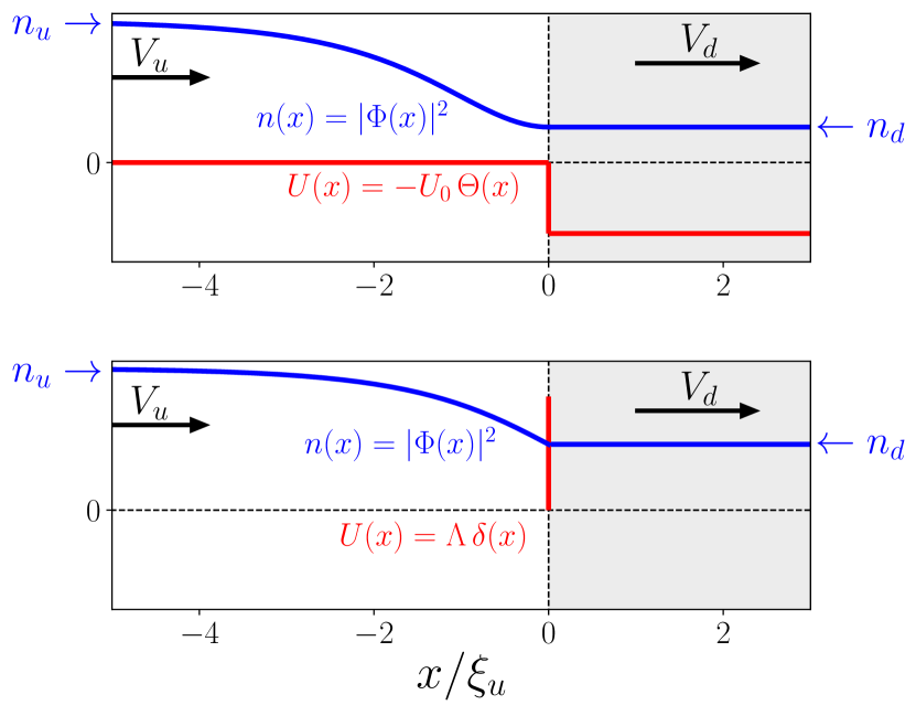
Figure 9: Schematic representation of the background density profile of the waterfall configuration (upper plot) and of the delta peak configuration (lower plot). The shaded region corresponds to the interior of the analog black hole (see the main text). The whole $x>0$ region is supersonic, while the upstream region is asymptotically subsonic (i.e., in the limit $x\to-\infty$).

Both configurations are depicted in Fig. 9. In this figure the region $x>0$ is shaded in order to remind that it corresponds to the interior of the analog black hole. It is however important to recall that the precise location of the horizon separating the interior and the exterior of an analog black hole is ill-defined, see, e.g., the discussion in Sec. II.A of Ref. [20].

Note that, while the upstream and downstream Mach numbers can be fixed independently in the flat profile configuration (with the only constrain that $m_{u}<1<m_{d}$), these two quantities are not independent in the waterfall and delta peak configurations:

$$m_{d}=m_{u}^{-2}\quad \mbox{for waterfall},$$ (37a)

$$\frac{m_{d}}{m_{u}}=\left(\frac{\displaystyle-1+\sqrt{1+8m_{u}^{-2}}}{\displaystyle 2}\right)^{3/2}\;$$ for delta peak. (37b)

Appendix B Covariance matrices

The $6\times 6$ covariante matrix $\sigma$ defined in Eq. (12) can be written in terms of $2\times 2$ submatrices $\sigma_{i}$ and $\varepsilon_{ij}$:

$$\sigma=\begin{pmatrix}\sigma_{0}&\varepsilon_{01}&\varepsilon_{02}\\ \varepsilon_{01}^{\rm\scriptscriptstyle T}&\sigma_{1}&\varepsilon_{12}\\ \varepsilon_{02}^{\rm\scriptscriptstyle T}&\varepsilon_{12}^{\rm\scriptscriptstyle T}&\sigma_{2}\end{pmatrix},$$ (38)

where

$$\sigma_{i}=\begin{pmatrix}\left\langle 2\hat{q}_{i}^{2}\right\rangle&\left\langle\hat{q}_{i}\,\hat{p}_{i}+\hat{p}_{i}\,\hat{q}_{i}\right\rangle\\ \left\langle\hat{q}_{i}\,\hat{p}_{i}+\hat{p}_{i}\,\hat{q}_{i}\right\rangle&\left\langle 2\hat{p}_{i}^{2}\right\rangle\\ \end{pmatrix},$$ (39)

and

$$\varepsilon_{ij}=2\,\begin{pmatrix}\left\langle\hat{q}_{i}\,\hat{q}_{j}\right\rangle&\left\langle\hat{q}_{i}\,\hat{p}_{j}\right\rangle\\ \left\langle\hat{p}_{i}\,\hat{q}_{j}\right\rangle&\left\langle\hat{p}_{i}\,\hat{p}_{j}\right\rangle\\ \end{pmatrix}.$$ (40)

In the case we consider, the definitions (13) and the specific form of the transformation (5) result in the following expressions:

$$\sigma_{i}=\left(1+2\,\langle\hat{c}_{i}^{\dagger}\hat{c}_{i}\rangle\right)\,\mathds{1}_{2},$$ (41)

$$\varepsilon_{01}=2\begin{pmatrix}\text{Re}\langle\hat{c}_{0}\,\hat{c}_{1}^{\dagger}\rangle&-\text{Im}\langle\hat{c}_{0}\,\hat{c}_{1}^{\dagger}\rangle\\ \text{Im}\langle\hat{c}_{0}\,\hat{c}_{1}^{\dagger}\rangle&\text{Re}\langle\hat{c}_{0}\,\hat{c}_{1}^{\dagger}\rangle\end{pmatrix},$$ (42)

and (for $i=0$ or 1)

$$\varepsilon_{i2}=2\begin{pmatrix}\text{Re}\left\langle\hat{c}_{i}\,\hat{c}_{2}\right\rangle&\text{Im}\left\langle\hat{c}_{i}\,\hat{c}_{2}\right\rangle\\ \text{Im}\left\langle\hat{c}_{i}\,\hat{c}_{2}\right\rangle&-\text{Re}\left\langle\hat{c}_{i}\,\hat{c}_{2}\right\rangle\end{pmatrix}.$$ (43)

In the limit of zero temperature the system is in a three mode pure Gaussian state. Its covariance matrix (38) can accordingly be brought by LLUBOs (local linear unitary Bogoliubov transformations) to a “standard form” in which matrices $\sigma_{i}$ are proportional to the identity [as they already are, cf. (41)] and matrices $\varepsilon_{ij}$ are diagonal [92, 80]. After this operation the matrices $\varepsilon_{ij}$ take the following form [20]

$$\varepsilon_{01}=2\,|\langle\hat{c}_{0}\,\hat{c}_{1}^{\dagger}\rangle|\mathds{1}_{2}\;,\;\;\varepsilon_{i2}=2\,|\langle\hat{c}_{i}\,\hat{c}_{2}\rangle|\,\sigma_{z},$$ (44)

where $i\in\{0,1\}$ and $\sigma_{z}$ is the third Pauli matrix.

The situation at finite temperature is less simple. The system is in a mixed state with no special symmetry, and the covariance matrix (38) cannot be put in a standard form where the matrices $\varepsilon_{ij}$ are all diagonal [80]. However, the situation simplifies again if one is interested in bipartite entanglement only (say, between modes $i$ and $j$). In this case one should trace out the third mode (let’s denote it by $k$) which simply amounts to remove from the total covariance matrix (38) the two rows and two columns where index $k$ appears. The remaining $4\times 4$ covariance matrix associated with the reduced two-mode state reads

$$\sigma^{(i|j)}=\begin{pmatrix}\sigma_{i}&\varepsilon_{ij}\\ \varepsilon_{ij}^{\rm\scriptscriptstyle T}&\sigma_{j}\end{pmatrix},$$ (45)

where the $2\times 2$ blocks are the same as the ones in (38). This reduced covariance matrix can always be brought by LLUBOs to its standard form [92], in which the matrix $\varepsilon_{ij}$ takes again the form (44) with here an average taken over the finite temperature state, as explained in the main text, Sec. II.2.

It has been argued in [20] that an efficient measure of bipartite entanglement was given by the “PPT measure” $\Lambda^{(i|j)}\equiv 1-\nu^{-}_{(i|j)}$ where $\nu^{-}_{(i|j)}$ is the lowest simplectic eigenvalue of the partial transpose of $\sigma^{(i|j)}$ . The largest entanglement corresponds to $\Lambda^{(i|j)}=1$ while separability is reached when $\Lambda^{(i|j)}<0$. This separability condition can be shown to be equivalent to the Peres-Horodecki criterion [95, 96]. Contrarily to other observables, such as the Cauchy-Schwarz criterion or the generalized Peres-Horodecki parameter which have been often used in the domain, the PPT measure has the advantage of being an entanglement monotone. Other observables have been used in the context of analog gravity, which are monotonous measures of entanglement, such as the entanglement entropy, the entanglement of formation or the logarithmic negativity, but they all have some drawbacks: the state our our system is mixed in a finite temperature situation, which discards the entanglement entropy as a possible measure. The entanglement entropy generalizes for mixed states to the entanglement of formation [97], but this quantity is not easily determined in non symmetric two-mode Gaussian states such as the ones we consider. The logarithmic negativity shares with the entanglement of formation the drawback of possibly violating monogamy inequalities [98]. This is a relatively mild drawback in the context of evaluating bipartite entanglement, but becomes prohibitive in the tripartite context. The Gaussian contangle was introduced in Ref. [98] as a quantity which has none of the previous deficiencies. It has been studied in the gravitational context [99] and also in analog gravity [20], but it is not of very practical use as its determination requires numerical minimisation of a complex expression. The PPT measure we use in the present study was introduced in Ref. [20] as a measure which mimics many aspects of the Gaussian contangle but is much simpler to evaluate. Its evaluation is as simple as the one of the above quoted quantities albeit it shares none of their drawbacks. The explicit expression of $\Lambda^{(i|2)}(\omega)$ characterizing the coupling between mode $i=0$ or $1$ and mode $j=2$ is given in Eq. (15) of the main text.

As clear from the above expressions (41), (42) and (43), the theoretical evaluation of the components of the covariance matrix relies on the computation of averages of two creation or annihilation operators of the outgoing modes. The relevant expressions are determined from Eq. (5) and read ($i=0$ or 1):

$$\begin{split}\langle\hat{c}^{\dagger}_{i}\hat{c}_{i}\rangle=&|S_{i0}|^{2}\bar{n}_{0}+|S_{i1}|^{2}\bar{n}_{1}+|S_{i2}|^{2}(1+\bar{n}_{2}),\\ \langle\hat{c}_{2}^{\dagger}\hat{c}_{2}\rangle=&|S_{20}|^{2}\bar{n}_{0}+|S_{21}|^{2}\bar{n}_{1}+|S_{22}|^{2}(1+\bar{n}_{2})-1,\\ \langle\hat{c}_{0}\hat{c}_{1}^{\dagger}\rangle=&S_{00}S_{10}^{*}\bar{n}_{0}+S_{01}S_{11}^{*}\bar{n}_{1}+S_{02}S_{12}^{*}(1+\bar{n}_{2}),\\ \langle\hat{c}_{i}\hat{c}_{2}\rangle=&S_{i0}S_{20}^{*}\bar{n}_{0}+S_{i1}S_{21}^{*}\bar{n}_{1}+S_{i2}S_{22}^{*}(1+\bar{n}_{2}),\\ \end{split}$$ (46)

where the $\bar{n}_{j}$’s ($j=0$, 1 or 2) are the occupation numbers of the incoming modes, see Eq. (14). The coefficients of the $S$ matrix appearing in the above formulae can be determined numerically as explained in Ref. [72]. Expressions (46) are useful for computing the PPT measure of entanglement (15) and the CHSH (19) and Svetlichny (21) parameters. As an illustration we now indicate how to compute the PPT measure $\Lambda^{(i|2)}$ at zero temperature. Using here the definition (54) as a short hand notation one gets from (15):

$$\begin{split}\Lambda^{(i|2)}(\omega)=&\sqrt{[|S_{i2}|^{2}+\sinh^{2}(r_{2})]^{2}+4|S_{i2}|^{2}}\\ &-|S_{i2}|^{2}-\sinh^{2}(r_{2}).\end{split}$$ (47)

It was shown in Ref. [72] that the ratio $|S_{i2}|^{2}/\sinh^{2}(r_{2})$ tends to a constant when $\omega\to 0$. Let’s denote $\Gamma_{i}$ the value of this constant ($i=0$ or 1) . A simple expansion of (47) shows that

$$\lim_{\omega\to 0}\Lambda^{(i|2)}=\frac{2\Gamma_{i}}{1+\Gamma_{i}}.$$ (48)

In the waterfall configuration [72]

$$\Gamma_{0}=\frac{4m_{u}}{(1+m_{u})^{2}},$$ (49)

and from relation (6) it follows that $\Gamma_{0}+\Gamma_{1}=1$. Hence, for the waterfall configuration

$$\lim_{\omega\to 0}\Lambda^{(0|2)}=\frac{8m_{u}}{1+6m_{u}+m_{u}^{2}},$$ (50a)

$$\lim_{\omega\to 0}\Lambda^{(1|2)}=\frac{(1-m_{u})^{2}}{1+m_{u}^{2}}.$$ (50b)

The maximum value of $\Lambda^{(0|2)}$ is always reached at $\omega=0$, thus the $T=0$ numerically determined value ${\rm max}_{\omega}\Lambda^{(0|2)}$ plotted in Fig. 4 is identical to (50a). The maximum value of the PPT measure of entanglement between modes 1 and 2 is reached at $\omega=0$ only for $m_{u}\lesssim 0.18$: the numerically determined value ${\rm max}_{\omega}\Lambda^{(1|2)}$ plotted in Fig. 4 is thus identical to (50b) in this range of values of $m_{u}$.

Appendix C An analogue optical system

As discussed in Ref. [20], the entanglement in the system can be localized by a transformation involving effective modes $\hat{f}_{0},\hat{f}_{1},\hat{f}_{2}$ schematically represented in Fig. 2. These modes are related to the physical outgoing modes by:

$$\hat{f}_{0} =-\sin\theta\,\hat{e}_{0}+\cos\theta\,\hat{e}_{1},$$ (51a)

$$\hat{f}_{1} =\cos\theta\,\hat{e}_{0}+\sin\theta\,\hat{e}_{1},$$ (51b)

$$\hat{f}_{2} =\hat{e}_{2},$$ (51c)

where

$$\hat{e}_{0}=\frac{S_{02}^{*}}{|S_{02}|}\,\hat{c}_{0},\,\,\hat{e}_{1}=\frac{S_{12}^{*}}{|S_{12}|}\,\hat{c}_{1},\,\,\hat{e}_{2}=\frac{S_{22}}{|S_{22}|}\,\hat{c}_{2},$$ (52)

with

$$\cos\theta=\frac{|S_{02}|}{\sinh r_{2}},\quad\sin\theta=\frac{|S_{12}|}{\sinh r_{2}},$$ (53)

and

$$r_{2}(\omega)=\operatorname{arsinh}\sqrt{|S_{22}|^{2}-1}.$$ (54)

It has been shown in Ref. [20] that an incoming vacuum mode of frequency $\omega$ relates to that of the effective $f$ modes by

$$|0_{\omega}\rangle^{\rm in}=\exp\left[r_{2}(\hat{f}_{1}^{\dagger}\,\hat{f}_{2}^{\dagger}-\hat{f}_{1}\,\hat{f}_{2})\right]|0_{\omega}\rangle^{f},$$ (55)

indicating that the $T=0$ state of the system is, as far as the $f_{1}$ and $f_{2}$ modes are concerned, a two-mode squeezed vacuum with squeezing parameter $r_{2}(\omega)$. The $f_{1}$ and $f_{2}$ modes are mixed by a beamsplitter (see Fig. 2) of transmission and reflection coefficients $\cos^{2}\theta$ and $\sin^{2}\theta$, respectively. It has been argued in Ref. [20] that the long wavelength limit of the transmission coefficient, $\Gamma_{0}=\lim_{\omega\to 0}\cos^{2}\theta$, plays the role of the grey-body factor of the analog black hole.

From definitions (51) and (52) and expressions (46) it is a simple matter to evaluate the following averages

$$\begin{split}&\langle\hat{f}_{0}^{\dagger}\hat{f}_{0}\rangle=\sum_{i=0}^{1}|S_{12}S_{0i}-S_{02}S_{1i}|^{2}\,\bar{n}_{i}/\sinh^{2}r_{2},\\ &\langle\hat{f}_{1}^{\dagger}\hat{f}_{1}\rangle=\cosh^{2}r_{2}\,\bar{n}_{01}+\sinh^{2}r_{2}(1+\bar{n}_{2}),\\ &\langle\hat{f}_{2}^{\dagger}\hat{f}_{2}\rangle=\sinh^{2}r_{2}\,\bar{n}_{01}+\cosh^{2}r_{2}(1+\bar{n}_{2})-1,\\ &\langle\hat{f}_{1}\hat{f}_{2}\rangle=\cosh r_{2}\sinh r_{2}(\bar{n}_{01}+\bar{n}_{2}+1).\\ \end{split}$$ (56)

The occupation numbers $\bar{n}_{j}$ ($j=0$, 1 or 2) in the above expressions are defined in (14) and use has been made of the shorthand notation

$$\bar{n}_{01}\equiv\frac{|S_{20}|^{2}}{\sinh^{2}r_{2}}\,\bar{n}_{0}+\frac{|S_{21}|^{2}}{\sinh^{2}r_{2}}\,\bar{n}_{1}.$$ (57)

It is quite informative to quantify the entanglement between the two effective modes $f_{1}$ and $f_{2}$ and the amount by which the corresponding squeezed state violates Bell inequality. At $T=0$ all the relevant quantities can be expressed in terms of the squeezing parameter (54) involved in the transformation (55). For instance, the analogues for the the modes $\hat{f}_{1}$ and $\hat{f}_{2}$, of the PPT measure of entanglement and of the CHSH parameter defined for the modes $\hat{c}_{i}$ and $\hat{c}_{2}$ by Eqs. (15) and (19), respectively, read

$$\Lambda^{(f_{1}|f_{2})}=1-\exp(-2r_{2}),$$ (58)

and [64]

$$B^{(f_{1}|f_{2})}=2\sqrt{1+\frac{4}{\pi^{2}}\arctan^{2}\left[\sinh(2r_{2})\right]}.$$ (59)

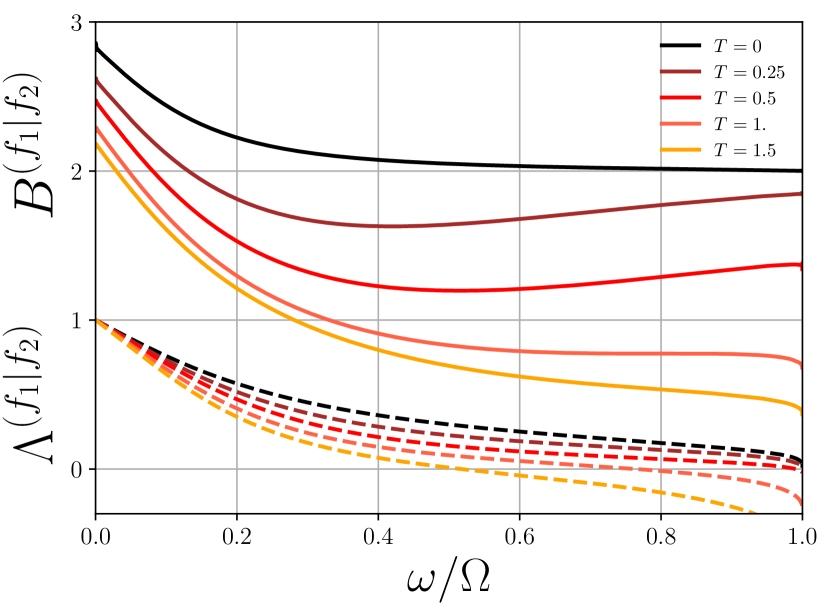
Figure 10: $B^{(f_{1}|f_{2})}$ (solid lines) and $\Lambda^{(f_{1}|f_{2})}$ (dashed lines) plotted as functions of $\omega$ for the two-mode squeeze state emulating the the waterfall configuration with $m_{d}=2.9$. The values of the different temperatures are indicated in units of $g\,n_{u}$.

The finite temperature values of these quantities can be obtained by replacing the $\hat{c}$ operators by the $\hat{f}$’s in expressions (15) and (101b) and using formulae (56). They are represented in Fig. 10 as functions of $\omega$ for a specific black hole configuration (waterfall with $m_{d}=2.9$). As anticipated, it appears that the violation of Bell inequality is here much more resilient to temperature than for the true Hawking-partner pair or the companion-partner pair (compare with Fig. 3). This is explained by the fact that the beam splitter distributes and, so to say, dilutes the entanglement. This is clear at $T=0$: in this case the $f_{0}$ mode is empty [cf. (56)] and the system is, as far as the $f$ modes are concerned, in a pure two-mode squeezed vacuum state. At $\omega=0$ for instance, the system is maximally entangled (the squeezing parameter $r_{2}\to\infty$) and both $\Lambda^{(f_{1}|f_{2})}$ and $B^{(f_{1}|f_{2})}$ reach their upper bounds (1 and $2\sqrt{2}$ respectively). At variance, if working with the true outgoing modes described by the $\hat{c}$ (or equivalently the $\hat{e}$) operators, for studying two-mode entanglement it is necessary to trace the (occupied) third one. The resulting density matrix is mixed, and in this case, entanglement and violation of Bell inequality are two different things, as clear from Fig. 3.

Another way to tackle this issue consists in expressing the PPT measure of entanglement (15) between the partner (mode 2) and mode $i$ ($i=0$ or 1) in terms of the parameters of the equivalent optical system. Denoting as $\gamma_{0}(\omega)=\cos^{2}\theta$ and $\gamma_{1}(\omega)=\sin^{2}\theta$ the transmission and reflection coefficient of the beam splitter makes it possible to write, at zero temperature, the PPT measure (15) under the form

$$\begin{split}\Lambda^{(i|2)}(\omega)&=(1+\gamma_{i})\sinh r_{2}\times\\ &\left\{\sqrt{\cosh^{2}r_{2}-\left(\frac{1-\gamma_{i}}{1+\gamma_{i}}\right)^{2}}-\sinh r_{2}\right\}.\end{split}$$ (60)

Algebraic manipulations then show that, because $\gamma_{i}\leq 1$, $\Lambda^{(i|2)}$ is always lower that $\Lambda^{(f_{1}|f_{2})}$. This means that the entanglement between modes $i$ and $2$ is always lower than the entanglement between the modes issued from the parametric down converted represented in Fig. 2. The equality is reached when $\gamma_{i}=1$, and, since $\gamma_{0}+\gamma_{1}=1$, in this case the other channel (let’s denote it as $\bar{\imath}=1-i$) is not entangled with mode 2: $\Lambda^{(\bar{\imath}|2)}=0$. So, indeed, the effect of the beam splitter is, so to say, to dispatch the entanglement of the effective squeezed modes $f_{1}$ and $f_{2}$ between modes $c_{0}$, $c_{1}$ and $c_{2}$.

After discussing two modes entanglement it is also interesting to briefly consider tripartite entanglement in the effective optical system depicted in Fig. 2. This system has been designed – by means of a procedure called entanglement localization [100] – in such a way that it concentrates entanglement between the effective squeezed modes $f_{1}$ and $f_{2}$. Therefore, it should be expected that, in the $f$ basis, the quantity $\langle\hat{\mathscr{S}}{}^{(f_{0}|f_{1}|f_{2})}\rangle$, which is sensible to a genuine tripartite nonlocality, will never reach values above two. Indeed, in this basis, at zero temperature one has

$$\langle\hat{\Pi}_{r}^{(f_{0})}\otimes\hat{\Pi}_{s}^{(f_{1})}\otimes\hat{\Pi}_{t}^{(f_{2})}\rangle=\langle\hat{\Pi}_{r}^{(f_{0})}\rangle\langle\hat{\Pi}_{s}^{(f_{1})}\otimes\hat{\Pi}_{t}^{(f_{2})}\rangle.$$ (61)

Since

$$\langle\hat{\Pi}_{z}^{(f_{0})}\rangle=1,\quad\langle\hat{\Pi}_{x}^{(f_{0})}\rangle=\langle\hat{\Pi}_{y}^{(f_{0})}\rangle=0,$$ (62)

it is legitimate to take, for evaluating expression (114) the vector ${\boldsymbol{a}}_{+}=\pm{\boldsymbol{e}}_{z}$ (taking $\boldsymbol{a}_{-}=\pm\boldsymbol{e}_{z}$ instead doesn’t change the result (64) below). This leads to

$$\begin{split}\text{max}_{\theta}\langle\hat{\mathscr{S}}{}^{(f_{0}|f_{1}|f_{2})}\rangle=\Big{|}\langle&\boldsymbol{b}\cdot\hat{\boldsymbol{\Pi}}{}^{(f_{1})}\otimes\boldsymbol{c}^{\prime}\cdot\hat{\boldsymbol{\Pi}}{}^{(f_{2})}\rangle\\ +&\langle\boldsymbol{b}^{\prime}\cdot\hat{\boldsymbol{\Pi}}{}^{(f_{1})}\otimes\boldsymbol{c}\cdot\hat{\boldsymbol{\Pi}}{}^{(f_{2})}\rangle\Big{|}.\end{split}$$ (63)

Then, noticing that at zero temperature $\langle\hat{\Pi}^{(f_{1})}_{z}\otimes\hat{\Pi}^{(f_{2})}_{z}\rangle=1$ at all energies and that the vector $\boldsymbol{b}$, $\boldsymbol{b}^{\prime}$, $\boldsymbol{c}$ and $\boldsymbol{c}^{\prime}$ are not constrained with respect to each other, one can take these vectors to be $+\boldsymbol{e}_{z}$, thus obtaining

$$S^{(f_{0}|f_{1}|f_{2})}(\omega)\underset{T=0}{=}2.$$ (64)

Of course the value of $S^{(f_{0}|f_{1}|f_{2})}$ decreases when the temperature increases. This quantity is thus always lower than 2, indicating, as expected, that there is no genuine tripartite nonlocality between the effective $f$ modes.

From Eqs. (61), (62) and also from the facts that $\langle\hat{\Pi}_{s}^{(f_{1})}\otimes\hat{\Pi}_{t}^{(f_{2})}\rangle=0$ if $s\neq t$ and that, at $\omega=0$ and $T=0$,

$$\langle\hat{\Pi}_{x}^{(f_{1})}\otimes\hat{\Pi}_{x}^{(f_{2})}\rangle=-\langle\hat{\Pi}_{y}^{(f_{1})}\otimes\hat{\Pi}_{y}^{(f_{2})}\rangle=1,$$ (65)

it is easily found that, at $\omega=0$, the optimized Mermin parameter (32) of the $f$ modes is

$$M^{(f_{0}|f_{1}|f_{2})}(0)\underset{T=0}{=}2.$$ (66)

This shows that, at variance with the $c$ modes, the effective $f$ modes do not violate the Mermin-Klyshko inequality and certainly do not exhibit the GHZ paradox. Results (64) and (66) were expected: since the $f$ modes do not exhibit tripartite entanglement they should violate none of the inequalities (34).

It follows from (49) that when $m_{u}=0$ or 1, at $\omega=0$, $\cos\theta=0$ or 1, respectively. In this case Eqs. (51), (52) and (53) indicate that the $f$ modes are connected to the $c$ modes by LLUBOs: the tripartite character of the true system thus disappears in these two limiting cases, even when $T=0$. However our results indicate that these two limits are singular, since the GHZ character of the system is observed (at $\omega=0$ and $T=0$) for all $m_{u}\in]0,1[$.

Appendix D Eigenstates of the pseudo-spin operators

In this appendix we list the properties of the eigenstates of the pseudo-spin operators (16) which are useful in the main text. We will consider a given one of the three modes ($j=0$, 1 or 2), always the same, and will omit the associated label $(j)$ in order to lighten the notations. In a similar way, we do not write the $\omega$-dependence which is implicit in all this appendix.

From the definition (16c) it follows that the matrix elements of $\hat{\Pi}_{z}$ between two number states are

$$\langle n|\hat{\Pi}_{z}|m\rangle=\left[(-)^{n}+(-)^{m}\right]\int_{0}^{\infty}{\rm d}q\,\psi_{n}(q)\psi_{m}(q),$$ (67)

where $\psi_{n}(q)=\langle n|q\rangle=(2^{n}n!\sqrt{\pi}\,)^{-1/2}\exp(-q^{2}/2)H_{n}(q)$ is a normalized Hermite function ($H_{n}$ a Hermite polynomial). The prefactor in the r.h.s. of (67) imposes that $n$ and $m$ have the same parity. Thus $\psi_{n}$ and $\psi_{m}$ are both even or odd functions of $q$, which makes it possible to extend by symmetry the integration range in the r.h.s. of (67) to the whole real axis, leading to

$$\langle n|\hat{\Pi}_{z}|m\rangle=(-)^{n}\delta_{n,m},$$ (68)

and thus

$$\hat{\Pi}_{z}=\sum_{n=0}^{\infty}\Big{(}|2n\rangle\langle 2n|-|2n+1\rangle\langle 2n+1|\Big{)}:$$ (69)

the eigenstates of $\hat{\Pi}_{z}$ are the number states, they have eigenvalue $\pm 1$ depending on their parity. In the following we will denote them as

$$|z^{+}_{n}\rangle=|2n\rangle,\quad\mbox{and}\quad|z^{-}_{n}\rangle=|2n+1\rangle.$$ (70)

Contrarily to usual spins 1/2, the two eigenvalues (here $+1$ and $-1$) are infinitely degenerate. This property is shared by any projection of the pseudo-spin operator; it is in particular true for the operator $\hat{\Pi}_{x}$. We denote the eigenstates of $\hat{\Pi}_{x}$ associated to the eigenvalue $\pm 1$ by $|x^{\pm}_{n}\rangle$, they can be constructed by rotating the eigenstates $|z^{\pm}_{n}\rangle$ of $\hat{\Pi}_{z}$ by angles $\pm\pi/2$ around the $y$ axis:

$$|x^{\pm}_{n}\rangle=\hat{\cal R}_{y}\left(\pm\frac{\pi}{2}\right)|z^{\pm}_{n}\rangle=\frac{1}{\sqrt{2}}\left(\mathds{1}\mp\hat{\Pi}_{y}\right)|z^{\pm}_{n}\rangle,$$ (71)

where $\hat{\cal R}_{y}(\theta)=\exp(-\frac{i}{2}\theta\,\hat{\Pi}_{y})$ is the operator of rotation of angle $\theta$ around the $y$ axis. The fact that $|x^{\pm}_{n}\rangle$ is an eigenstate of $\hat{\Pi}_{x}$ with eigenvalue $\pm 1$ is easily checked by direct application of $\hat{\Pi}_{x}$ to the left of expression (71) and use of the relations

$$\hat{\Pi}_{r}\hat{\Pi}_{s}=i\,\varepsilon_{rst}\,\hat{\Pi}_{t},$$ (72)

where $\varepsilon_{rst}$ is the totally antisymmetric Levi-Civita symbol and $(r,s,t)=x$, $y$ or $z$. By the same token it is also easily proven that

$$\hat{\Pi}_{y}|x^{\pm}_{n}\rangle=\mp i|x^{\mp}_{n}\rangle,\quad\mbox{and}\quad\hat{\Pi}_{z}|x^{\pm}_{n}\rangle=|x^{\mp}_{n}\rangle.$$ (73)

Appendix E Computing expectation values of observables

The use of the technique of Wigner transform is particularly well suited for determining the different contributions of the pseudo-spin operator to the CHSH measures (19) and (21). The reason is twofold: first, we consider a Gaussian state and for computing the required averages we thus just need to evaluate Gaussian integrals weighted by the Wigner transforms of the spin operators and secondly, the Wigner transforms of the pseudo-spins (16) are simple enough that the relevant integrals can be evaluated analytically.

We will consider $n=3$ (and also $n=2$) modes Gaussian states and the computation of the average of an operator $\hat{A}$ is performed in an abstract dimensional phase space according to

$$\langle\hat{A}\rangle=\int{\rm d}^{n}\boldsymbol{q}{\rm d}^{n}\boldsymbol{p}\,W_{\hat{\rho}}(\boldsymbol{q},\boldsymbol{p})\,W_{\!\!\hat{A}}(\boldsymbol{q},\boldsymbol{p}).$$ (74)

In this expression $W_{\hat{\rho}}$ is the Wigner transform of the density matrix. In the Gaussian case we consider it can be computed from the knowledge of the covariance matrix [101]:

$$W_{\hat{\rho}}(\boldsymbol{q},\boldsymbol{p})=\frac{1}{\pi^{n}\sqrt{{\rm det}\sigma}}\exp\{-\tfrac{1}{2}\boldsymbol{\xi}^{\rm\scriptscriptstyle T}\sigma^{-1}\boldsymbol{\xi}\},$$ (75)

where $\sigma$ is the total (or reduced, as appropriate) covariance matrix defined in Eq. (12). In this expression, $n=3$ and $\boldsymbol{\xi}=\sqrt{2}\,(q_{0},p_{0},q_{1},p_{1},q_{2},p_{2})^{\rm\scriptscriptstyle T}$ in the three-mode case. In the reduced two-mode case, $n=2$ and one should remove from the expression of $\boldsymbol{\xi}$ the entries corresponding to the subscript of the traced mode. The Wigner transform (75) of a Gaussian state is non-negative, and it was originally considered impossible to violate Bell’s inequality under such conditions [102]. This was latter proven incorrect [103, 104]. In particular, Revzen et al. [105] proved that observables can be associated to the violation of Bell inequality over a Gaussian state provided their Wigner transform takes values different from the eigenvalues of the associated quantal operator. We will see that the pseudo-spins (16) we consider belong to this class of observables, denoted as “improper” in Ref. [105].

The other term involved in the integration (74) is the Wigner transform $W_{\!\!\hat{A}}$ of the operator $\hat{A}$. It is a function defined in phase space by means of an integration over “representation space”

$$W_{\!\!\hat{A}}(\boldsymbol{q},\boldsymbol{p})=\int{\rm d}^{n}\boldsymbol{z}\exp\{i\boldsymbol{p}\cdot\boldsymbol{z}\}\langle\boldsymbol{q}-\tfrac{1}{2}\boldsymbol{z}|\hat{A}|\boldsymbol{q}+\tfrac{1}{2}\boldsymbol{z}\rangle.$$ (76)

In this expression $\boldsymbol{q}$ (as well as $\boldsymbol{z}$ and $\boldsymbol{p}$) is a vector in an abstract $n=3$ dimensional space (with basis $\boldsymbol{e}_{0},\boldsymbol{e}_{1},\boldsymbol{e}_{2}$). The kets involved in (76) are of the type $|\boldsymbol{Q}\rangle=|Q_{0}\rangle_{0}\otimes|Q_{1}\rangle_{1}\otimes|Q_{2}\rangle_{2}$ where $\boldsymbol{Q}=Q_{0}\boldsymbol{e}_{0}+Q_{1}\boldsymbol{e}_{1}+Q_{2}\boldsymbol{e}_{2}$ and $|Q\rangle_{j}$ is the eigenstate of operator $\hat{q}_{j}$ associated to the eigenvalue $Q$ ($j=0$, 1 or 2). In the case of a reduced two modes Gaussian state $n=2$ and the vector $\boldsymbol{Q}$ is two-dimensional: the component associated to the traced mode disappears, as it also does in $|\boldsymbol{Q}\rangle$.

For evaluating expectation values such as those appearing in Eqs. (19) and (21) we need to compute the Wigner transforms of the components of the pseudo-spin operators. These are to be evaluated in a 2 dimensional phase space, since operator $\hat{\boldsymbol{\Pi}}{}^{(j)}$ concerns a single mode (mode $j$). The result is independent of $j$ and reads:

$$\begin{split}W_{\hat{\Pi}_{x}}(q,p)=&\mbox{sgn}\,(q),\\ W_{\hat{\Pi}_{y}}(q,p)=&i\delta(q)\int_{-\infty}^{\infty}\!\!{\rm d}x\,\mbox{sgn}\,(x)\exp\{-2ipx\}\\ =&\delta(q){\cal P}(1/q),\\ W_{\hat{\Pi}_{z}}(q,p)=&\pi\delta(q)\delta(p),\end{split}$$ (77)

where ${\cal P}$ denotes the principal value. It is shown in the main text that the eigenvalues of the projections along a given axis of the pseudo-spin operator $\hat{\boldsymbol{\Pi}}$ are $\pm 1$. The above expressions of the Wigner transforms thus demonstrate that, contrarily to $\hat{\Pi}_{x}$, operators $\hat{\Pi}_{y}$ and $\hat{\Pi}_{z}$ are “improper” in the sense of Ref. [105]: they may be involved in violation of Bell inequality even for a state with a non-negative Wigner transform, such as the Gaussian state we consider.

For evaluating the expectation values appearing in (19) we need to compute integrals such as

$$\begin{split}\langle\hat{\Pi}^{(i)}_{z}\otimes\hat{\Pi}^{(2)}_{z}\rangle=\int&\!{\rm d}^{2}\boldsymbol{q}{\rm d}^{2}\boldsymbol{p}\,W_{\hat{\Pi}_{z}}(q_{i},p_{i})\times\\ &W_{\hat{\Pi}_{z}}(q_{2},p_{2})W_{\hat{\rho}}(\boldsymbol{q},\boldsymbol{p}),\end{split}$$ (78)

where $\boldsymbol{q}=(q_{i},q_{2})$ and $\boldsymbol{p}=(p_{i},p_{2})$ ($i=0$ or 1). The explicit calculation yields

$$\langle\hat{\Pi}^{(i)}_{z}\otimes\hat{\Pi}^{(2)}_{z}\rangle=\frac{1}{a_{i}a_{2}-4|\langle\hat{c}_{i}\hat{c}_{2}\rangle|^{2}},$$ (79)

where

$$a_{j}=2\langle\hat{c}^{\dagger}_{j}\hat{c}_{j}\rangle+1$$ (80)

is known as the local mixedness of mode $j$ ($j=0,1$ or 2). The other terms involved in the determination of the CHSH parameter (19) can be evaluated by the same technique. The computation is similar to the one figuring in the Appendix of Ref. [59]. One finds that all expectation values for which the index $z$ appears a single time cancel at all temperatures. The values of the other non-zero averages are ($i=0$ or 1):

$$\begin{split}\langle\hat{\Pi}^{(i)}_{x}\otimes\hat{\Pi}^{(2)}_{x}\rangle=&\frac{2}{\pi}\arctan\frac{2\,\mbox{Re}\,\langle\hat{c}_{i}\hat{c}_{2}\rangle}{\sqrt{a_{i}a_{2}-4(\mbox{Re}\,\langle\hat{c}_{i}\hat{c}_{2}\rangle)^{2}}},\\ \langle\hat{\Pi}^{(i)}_{y}\otimes\hat{\Pi}^{(2)}_{y}\rangle=&\frac{-1}{A_{i2}}\langle\hat{\Pi}^{(i)}_{x}\otimes\hat{\Pi}^{(2)}_{x}\rangle,\\ \langle\hat{\Pi}^{(i)}_{x}\otimes\hat{\Pi}^{(2)}_{y}\rangle=&\frac{2}{\pi\,a_{2}}\operatorname{arsinh}\frac{2\,\mbox{Im}\,\langle\hat{c}_{i}\hat{c}_{2}\rangle}{\sqrt{A_{i2}}},\\ \langle\hat{\Pi}^{(i)}_{y}\otimes\hat{\Pi}^{(2)}_{x}\rangle=&\frac{2}{\pi\,a_{i}}\operatorname{arsinh}\frac{2\,\mbox{Im}\,\langle\hat{c}_{i}\hat{c}_{2}\rangle}{\sqrt{A_{i2}}},\\ \end{split}$$ (81)

where $A_{i2}$ is defined in Eq. (83) below, and we recall that the expression of the quantity $\langle\hat{c}_{i}\hat{c}_{2}\rangle$ is given in (46).

For studying the Svetlichny observable it is necessary to evaluate averages involving the Cartesian coordinates of three pseudo-spins, of the type

$${\cal T}_{rst}(\omega)\equiv\left\langle\hat{\Pi}^{(0)}_{r}\otimes\hat{\Pi}^{(1)}_{s}\otimes\hat{\Pi}^{(2)}_{t}\right\rangle,$$ (82)

where $r$, $s$ and $t\in\{x,y,z\}$. These quantities are zero if $z$ is not one of the indices or appears exactly twice. In order to write down tractable expressions in the other cases, it is convenient to introduce new compact notations:

$$\begin{split}A_{01}=&a_{0}a_{1}-4\,|\langle\hat{c}_{0}\hat{c}_{1}^{\dagger}\rangle|^{2},\\ A_{i2}\underset{i<2}{=}&a_{i}a_{2}-4\,|\langle\hat{c}_{i}\hat{c}_{2}\rangle|^{2},\end{split}$$ (83)

$$\begin{split}&Z_{0}=-2a_{0}\langle\hat{c}_{1}\hat{c}_{2}\rangle^{*}+4\langle\hat{c}_{0}\hat{c}_{1}^{\dagger}\rangle\langle\hat{c}_{0}\hat{c}_{2}\rangle^{*},\\ &Z_{1}=-2a_{1}\langle\hat{c}_{0}\hat{c}_{2}\rangle^{*}+4\langle\hat{c}_{0}\hat{c}_{1}^{\dagger}\rangle^{*}\langle\hat{c}_{1}\hat{c}_{2}\rangle^{*},\\ &Z_{2}=-2a_{2}\langle\hat{c}_{0}\hat{c}_{1}^{\dagger}\rangle^{*}+4\langle\hat{c}_{1}\hat{c}_{2}\rangle\langle\hat{c}_{0}\hat{c}_{2}\rangle^{*},\end{split}$$ (84)

and

$$\begin{split}\delta=&a_{0}a_{1}a_{2}+16\,\mbox{Re}\left\{\langle\hat{c}_{0}\hat{c}^{\dagger}_{1}\rangle\langle\hat{c}_{1}\hat{c}_{2}\rangle\langle\hat{c}_{0}\hat{c}_{2}\rangle^{*}\right\}\\ &-4a_{0}|\langle\hat{c}_{1}\hat{c}_{2}\rangle|^{2}-4a_{1}|\langle\hat{c}_{0}\hat{c}_{2}\rangle|^{2}-4a_{2}|\langle\hat{c}_{0}\hat{c}^{\dagger}_{1}\rangle|^{2}.\end{split}$$ (85)

$\delta$ is the square of the determinant of the $6\times 6$ covariance matrix (38). At $T=0$ the system is in a pure state and $\delta=1$ for all values of $\omega$ [106], whereas $\delta={\cal O}(1/\omega)$ at finite temperature, as can be shown on the basis of the low energy expansion of the matrix elements of the $S$-matrix given in Ref. [72].

The explicit theoretical evaluation of the quantities (80), (83), (84) and (85) is easily done from Eqs. (46). A long computation shows that the averages (82) which are non zero can be expressed in terms of these quantities:

$$\begin{split}&{\cal T}_{zxx}=-\frac{2}{\pi a_{0}}\arctan\frac{\mbox{Re}\,Z_{0}}{\sqrt{A_{01}A_{02}-(\mbox{Re}\,Z_{0})^{2}}},\\ &{\cal T}_{xzx}=-\frac{2}{\pi a_{1}}\arctan\frac{\mbox{Re}\,Z_{1}}{\sqrt{A_{01}A_{12}-(\mbox{Re}\,Z_{1})^{2}}},\\ &{\cal T}_{xxz}=-\frac{2}{\pi a_{2}}\arctan\frac{\mbox{Re}\,Z_{2}}{\sqrt{A_{02}A_{12}-(\mbox{Re}\,Z_{2})^{2}}},\end{split}$$ (86)

$$\begin{split}&{\cal T}_{zyy}=-\frac{a_{0}}{\delta}{\cal T}_{zxx},\quad{\cal T}_{yzy}=-\frac{a_{1}}{\delta}{\cal T}_{xzx},\\ &{\cal T}_{yyz}=+\frac{a_{2}}{\delta}{\cal T}_{xxz},\end{split}$$ (87)

$$\begin{split}A_{02}{\cal T}_{zxy}=A_{01}{\cal T}_{zyx}=&\operatorname{arsinh}\left(\frac{\mbox{Im}\,Z_{0}}{\sqrt{a_{0}\delta}}\right),\\ A_{01}{\cal T}_{yzx}=A_{12}{\cal T}_{xzy}=&\operatorname{arsinh}\left(\frac{\mbox{Im}\,Z_{1}}{\sqrt{a_{1}\delta}}\right),\\ -A_{12}{\cal T}_{xyz}=A_{02}{\cal T}_{yxz}=&\operatorname{arsinh}\left(\frac{\mbox{Im}\,Z_{2}}{\sqrt{a_{2}\delta}}\right),\end{split}$$ (88)

and

$${\cal T}_{zzz}=\frac{1}{\delta}.$$ (89)

The low energy behavior of the quantities (86) is dictated by the one of the local mixednesses $a_{0}$, $a_{1}$ and $a_{2}$ which diverge as $1/\omega$ for all temperature. As a result

$$\lim_{\omega\to 0}{\cal T}_{zxx}=\lim_{\omega\to 0}{\cal T}_{xzx}=\lim_{\omega\to 0}{\cal T}_{xxz}\underset{\forall T}{=}0.$$ (90)

On the other hand, the behavior of the quantities (87) depends on the behavior of the (square root $\delta$ of the) determinant of the covariance matrix which is unity at $T=0$ [106]. In this case

$${\cal T}_{zzz}(\omega)\underset{T=0}{=}1,$$ (91)

and

$$\lim_{\omega\to 0}{\cal T}_{zyy}=\lim_{\omega\to 0}{\cal T}_{yzy}=\lim_{\omega\to 0}{\cal T}_{yyz}\underset{T=0}{=}1.$$ (92)

The reason for this behavior is that, at $T=0$, $\delta=1$ whereas the arguments of all the $\arctan$ terms in (86) diverge as $\omega^{-1/2}$, as shown by detailed inspection based on Eqs. (83), (84), (46) and the asymptotic expression of the coefficients of the $S$ matrix given in [72].

Alternatively, at finite temperature $\delta$ diverges at low energy (as $1/\omega$) and the limits (92) all cancel

$$\lim_{\omega\to 0}{\cal T}_{zyy}=\lim_{\omega\to 0}{\cal T}_{yzy}=\lim_{\omega\to 0}{\cal T}_{yyz}\underset{T\neq 0}{=}0,$$ (93)

as also does $\lim_{\omega\to 0}{\cal T}_{zzz}\underset{T\neq 0}{=}0$.

Appendix F Analytic maximization of $\langle\hat{\mathscr{B}}{}^{(i|2)}\rangle$

In this appendix we present the maximisation of the expectation value of the CHSH operator (18). We only state the results useful for the main text but do not detail the procedure because it is well known, see e.g., Refs. [107, 108]. In particular, it can be shown that the CHSH parameter $B^{(i|2)}(\omega)$ defined in (19) reads

$$B^{(i|2)}=2\sqrt{\lambda_{1}+\lambda_{2}}\,,$$ (94)

where $\lambda_{1}$ and $\lambda_{2}$ are the two largest eigenvalues of matrix ${}^{\rm\scriptscriptstyle T}{\cal T}\,{\cal T}$ where ${\cal T}(\omega)$ is the $3\times 3$ matrix with entries

$${\cal T}_{rs}=\left\langle\hat{\Pi}^{(i)}_{r}\otimes\hat{\Pi}^{(2)}_{s}\right\rangle,$$ (95)

with $(r,s)\in\{x,y,z\}^{2}$. The results presented in Appendix E show that in all the cases we consider the matrix ${\cal T}(\omega)$ is block diagonal:

$${\cal T}=\begin{pmatrix}{\cal T}_{xx}&{\cal T}_{xy}&0\\ {\cal T}_{yx}&{\cal T}_{yy}&0\\ 0&0&{\cal T}_{zz}\\ \end{pmatrix},$$ (96)

and thus

$$^{\rm\scriptscriptstyle T}{\cal T}\,{\cal T}=\begin{pmatrix}A&C&0\\ C&B&0\\ 0&0&{\cal T}^{2}_{zz}\\ \end{pmatrix},$$ (97)

with

$$\begin{split}A&={\cal T}_{xx}^{2}+{\cal T}_{yx}^{2},\quad B={\cal T}_{yy}^{2}+{\cal T}_{xy}^{2},\\ C&={\cal T}_{xx}{\cal T}_{xy}+{\cal T}_{yy}{\cal T}_{yx}.\end{split}$$ (98)

The largest eigenvalues of matrix ${}^{\rm\scriptscriptstyle T}{\cal T}\,{\cal T}$ are ${\cal T}_{zz}^{2}$ and

$$\frac{1}{2}\left(A+B+\sqrt{(A-B)^{2}+4C^{2}}\right).$$ (99)

They can be computed from Expressions (79), (81) and (98). Then Eq. (94) determines the value of the CHSH parameter (19).

One may also chose a different strategy for attempting to maximise the expectation value of the operator $\mathscr{B}^{(i|2)}$. Instead of choosing to work in the basis of the $c$- modes, one may perform a LLUBO for attempting to simplify the form of the covariance matrix. As already stated in Appendix B, in the bipartite case, the $4\times 4$ covariance matrix (45) associated with the reduced two-mode state $(i|2)$ can be brought by LLUBOs to a standard form where the matrix $\varepsilon_{i2}$ are diagonal [92]. Working in this basis does not alter the entanglement properties of the system (they remain unaffected compared to that of the $c$-modes), but makes the computations easier and may improve the signal of nonlocality. In this basis the result (79) is not affected and expressions (81) modify to

$$\begin{split}{\cal T}_{xx}=\;&\frac{2}{\pi}\arctan\frac{2\,|\langle\hat{c}_{i}\hat{c}_{2}\rangle|}{\sqrt{A_{i2}}}=-A_{i2}{\cal T}_{yy},\\ {\cal T}_{xy}=\;&{\cal T}_{yx}=0,\\ \end{split}$$ (100)

where $A_{i2}$ is defined in Eq. (83). The matrix ${\cal T}$ is thus diagonal and expression (99) is equal to ${\cal T}_{xx}^{2}$. Equation (94) then reads

$$B^{(i|2)}= 2\,\sqrt{{\cal T}_{xx}^{2}+{\cal T}_{zz}^{2}}$$ (101a)

$$= 2\,\sqrt{\frac{4}{\pi^{2}}\arctan^{2}\left(\frac{2|\langle\hat{c}_{i}\hat{c}_{2}\rangle|}{\sqrt{A_{i2}}}\right)+\frac{1}{A_{i2}^{2}}}\,.$$ (101b)

We note here that the difference between the result (94) evaluated in the $c$-mode basis and expression (101b) is always small. The reason is that, in the $c$-mode basis, the off diagonal entries of the upper left blocks of matrix (96) and (97) are always small compared to the diagonal ones, because at all temperature $|\mbox{Im}\,\langle\hat{c}_{i}\hat{c}_{2}\rangle|\ll|\mbox{Re}\,\langle\hat{c}_{i}\hat{c}_{2}\rangle|$. However, our numerical checks always demonstrate a small increase of the Bell parameter (101b) compared to the one evaluated using (94) in the $c$-mode basis. We thus present our numerical results in Figs. 3, 4, 5, 10, 11 and 12 using formula (101b). To summarize, the result (101b) should be considered as an optimized value of the witness of nonlocality $B^{(i|2)}$. We note here that we do not have a general proof of the better efficiency of the method which consists in using the basis in which the covariance matrix is in its standard form, but we believe that a general mathematical result of this type would be quite useful.

Appendix G Numerical maximization of $\langle\hat{\mathscr{S}}{}^{(0|1|2)}\rangle$

As explained in Sec. IV, the maximal value of the three-mode Bell operator $\langle\hat{\mathscr{S}}{}^{(0|1|2)}\rangle$ can be found by optimizing the orientation of the unit vectors $\boldsymbol{a}$, $\boldsymbol{a}^{\prime}$, $\boldsymbol{b}$, $\boldsymbol{b}^{\prime}$, $\boldsymbol{c}$ and $\boldsymbol{c}^{\prime}$. However, solving this optimization problem analytically proves challenging due to the need to maximize a function depending on 12 real parameters. Indeed, the orientation of each of the six previous normalized vectors in the 3-dimensional physical space corresponds to two degrees of freedom, leading in total to twelve parameters.

Consequently, we resort to a numerical method to evaluate the maximal violation of Bell inequalities and determine the corresponding optimal orientations for the vectors $\boldsymbol{a}$, $\boldsymbol{a}^{\prime}$, $\boldsymbol{b}$, $\boldsymbol{b}^{\prime}$, $\boldsymbol{c}$, and $\boldsymbol{c}^{\prime}$. More explicitly, we use a genetic algorithm which has proved very efficient for optimizing a function over a large parameter space [109]. This algorithm is based on natural selection: the code starts with a random set of solutions (in our case each of them consists of 12 parameters) which form all together what we call a population. We then compute, for each set of vectors ($\boldsymbol{a},\boldsymbol{a}^{\prime},\boldsymbol{b},\boldsymbol{b}^{\prime},\boldsymbol{c},\boldsymbol{c}^{\prime}$), the expectation value $\langle\hat{\mathscr{S}}{}^{(0|1|2)}\rangle$ by means of the technique exposed in Appendix E. For instance the contribution of the term $\langle\boldsymbol{a}\cdot\hat{\boldsymbol{\Pi}}{}^{(0)}\otimes\boldsymbol{b}\cdot\hat{\boldsymbol{\Pi}}{}^{(1)}\otimes\boldsymbol{c}\cdot\hat{\boldsymbol{\Pi}}{}^{(2)}\rangle$ to $\langle\hat{\mathscr{B}}{}^{(0|1|2)}\rangle$ can be evaluated from the knowledge of the terms ${\cal T}_{rst}$ defined in Eq. (82):

$$\langle\boldsymbol{a}\cdot\hat{\boldsymbol{\Pi}}{}^{(0)}\otimes\boldsymbol{b}\cdot\hat{\boldsymbol{\Pi}}{}^{(1)}\otimes\boldsymbol{c}\cdot\hat{\boldsymbol{\Pi}}{}^{(2)}\rangle=\sum_{r,s,t}a_{r}b_{s}c_{t}{\cal T}_{rst},$$ (102)

where the sum runs over the indices $(r,s,t)\in\{x,y,z\}^{3}$. At variance with the bipartite case, at finite temperature it not not possible to find a LLUBO enabling to cast the $6\times 6$ covariance matrix (38) under a standard form where all the $\varepsilon_{ij}$ matrices are diagonal (see the discussion in Appendix B). The expectation values are thus computed in the natural basis of the $c$-modes where the values of the ${\cal T}_{rst}$ coefficients are given by Eqs. (86), (87), (88) and (89).

At each step of the algorithm the code computes the expectation value $\langle\hat{\mathscr{S}}{}^{(0|1|2)}\rangle$ for a set of vectors ($\boldsymbol{a},\boldsymbol{a}^{\prime},\boldsymbol{b},\boldsymbol{b}^{\prime},\boldsymbol{c},\boldsymbol{c}^{\prime}$) and ranks the members of the population by computing a fitness scaling function, a kind of selection rule: only the members of the population with the lowest fitness value will be retained – they are called the parents – and used to generate new sets of solutions, called the children. Then, at the next step, the selection rules are applied to the children, some of them become parents in turn and engender a new generation. The algorithm stops when all children look like their parents, or, in other words, when

$$|\boldsymbol{v}_{\ell+1}-\boldsymbol{v}_{\ell}|<\delta,$$ (103)

where $\boldsymbol{v}_{\ell}=(\boldsymbol{a},\boldsymbol{a}^{\prime},\boldsymbol{b},\boldsymbol{b}^{\prime},\boldsymbol{c},\boldsymbol{c}^{\prime})$ is the set of solutions at step $\ell$ of the algorithm, and $\delta$ is the chosen convergence precision fixed prior the beginning of the selection process.

In our case, the fitness scaling function is simply the opposite of the average $\langle\hat{\mathscr{S}}{}^{(0|1|2)}\rangle$ of the three-mode Bell operator. Trying to obtain the lowest fitness score is thus equivalent to maximize the Bell operator. For a given set of vectors $\boldsymbol{v}_{\ell}$ at step $\ell$, the next generation is computed as follows: $\boldsymbol{v}_{\ell+1}=\boldsymbol{v}_{\ell}+\boldsymbol{w}_{\ell}$, where $\boldsymbol{w}_{\ell}$ is a random weight which controls the mutations between the parents $\boldsymbol{v}_{\ell}$ and the children $\boldsymbol{v}_{\ell+1}$, and which tends to decrease when the code starts to converge. For a detailed presentation of the algorithm we refer to Ref. [110]. Note finally that the procedure just presented is also used for determining the optimized Mermin parameter (32).

Appendix H Tripartite Cirel’son bound and analytic maximization of $\langle\hat{\mathscr{S}}{}^{(0|1|2)}(\omega=0)\rangle$

In this section we first study the upper bound of the quantity $S^{(0|1|2)}(\omega)$ defined in (21) and then study the possibility of maximisation of the average $\langle\hat{\mathscr{S}}{}^{(0|1|2)}\rangle$ of the operator (20) by an appropriate choice of the measurement directions $\boldsymbol{a}$, $\boldsymbol{a}^{\prime}$, $\boldsymbol{b}$, $\boldsymbol{b}^{\prime}$, $\boldsymbol{c}$ and $\boldsymbol{c}^{\prime}$.

Denoting as $\hat{A}=\boldsymbol{a}\cdot\hat{\boldsymbol{\Pi}}{}^{(0)}$, $\hat{A}^{\prime}=\boldsymbol{a}^{\prime}\cdot\hat{\boldsymbol{\Pi}}{}^{(0)}$, $\hat{B}=\boldsymbol{b}\cdot\hat{\boldsymbol{\Pi}}{}^{(1)}$, etc. makes it possible to write the square of the tripartite Svetlichny operator (20) as

$$\begin{split}4\left(\hat{\mathscr{S}}{}^{(0|1|2)}\right)^{2}=&8+\{\hat{A},\hat{A}^{\prime}\}\otimes\{\hat{B},\hat{B}^{\prime}\}\otimes\{\hat{C},\hat{C}^{\prime}\}\\ &-2[\hat{A},\hat{A}^{\prime}]\otimes[\hat{B},\hat{B}^{\prime}]\otimes\mathds{1}^{(2)}\\ &-2\mathds{1}^{(0)}\otimes[\hat{B},\hat{B}^{\prime}]\otimes[\hat{C},\hat{C}^{\prime}]\\ &-2[\hat{A},\hat{A}^{\prime}].\otimes\mathds{1}^{(1)}\otimes[\hat{C},\hat{C}^{\prime}],\end{split}$$ (104)

where $[\cdot,\cdot]$ and $\{\cdot,\cdot\}$ denote the commutator ans the anticommutator, respectively. From the SU(2) algebra of the pseudo-spins it is easily proven that

$$[\hat{A},\hat{A}^{\prime}] =2i(\boldsymbol{a}\times\boldsymbol{a}^{\prime})\cdot\hat{\boldsymbol{\Pi}}{}^{(0)},$$ (105a)

$$\{\hat{A},\hat{A}^{\prime}\} =2(\boldsymbol{a}\cdot\boldsymbol{a}^{\prime})\mathds{1}^{(0)},$$ (105b)

with similar formulae for the quantities $\hat{B}$, $\hat{B}^{\prime}$ and $\hat{C}$, $\hat{C}^{\prime}$. Since the operators $\hat{A}$, $\hat{B}$ and $\hat{C}$ operate in different Hilbert spaces, one can assume without loss of generality that all the vector products of type (105a) appearing in (104) are colinear with $\boldsymbol{e}_{z}$. In this case all the unit vectors $\boldsymbol{a}$, $\boldsymbol{a}^{\prime}$, $\boldsymbol{b}$, $\boldsymbol{b}^{\prime}$, $\boldsymbol{c}$ and $\boldsymbol{c}^{\prime}$ lie in the $xy$ plane. Denoting as $\theta_{a}$ the angle between $\boldsymbol{a}^{\prime}$ and $\boldsymbol{a}$, $\theta_{b}$ the angle between $\boldsymbol{b}^{\prime}$ and $\boldsymbol{b}$, and $\theta_{c}$ the angle between $\boldsymbol{c}^{\prime}$ and $\boldsymbol{c}$ (all these angles being in $[0,\pi]$), one gets

$$\begin{split}\left(\hat{\mathscr{S}}{}^{(0|1|2)}\right)^{2}=&2+2\cos\theta_{a}\cos\theta_{b}\cos\theta_{c}\\ &+2\sin\theta_{a}\sin\theta_{b}\,\hat{\Pi}_{z}^{(0)}\otimes\hat{\Pi}_{z}^{(1)}\otimes\mathds{1}^{(2)}\\ &+2\sin\theta_{b}\sin\theta_{c}\,\mathds{1}^{(0)}\otimes\hat{\Pi}_{z}^{(1)}\otimes\hat{\Pi}_{z}^{(2)}\\ &+2\sin\theta_{a}\sin\theta_{c}\,\hat{\Pi}_{z}^{(0)}\otimes\mathds{1}^{(1)}\otimes\hat{\Pi}_{z}^{(2)}.\end{split}$$ (106)

It is a simple matter to check that when $\theta_{a}$, $\theta_{b}$ and $\theta_{c}$ run through $[0,2\pi]^{3}$ the eigenvalues of the operator appearing in the right hand side of the above formula are all comprised in $[0,8]$. The extremal values 0 and 8 are reached for $(\theta_{a},\theta_{b},\theta_{c})=(0,0,\pi)$ and $(\pi/2,\pi/2,\pi/2)$, respectively. It then follows that for any choice of the measurement directions $\boldsymbol{a}$, $\boldsymbol{a}^{\prime}$, $\boldsymbol{b}$, $\boldsymbol{b}^{\prime}$, $\boldsymbol{c}$ and $\boldsymbol{c}^{\prime}$

$$\left\langle\hat{\mathscr{S}}{}^{(0|1|2)}\right\rangle^{2}\leq\left\langle(\hat{\mathscr{S}}{}^{(0|1|2)})^{2}\right\rangle\leq 8,$$ (107)

and thus the tripartite entanglement parameter (21) verifies

$$S^{(0|1|2)}(\omega)\leq 2\sqrt{2}.$$ (108)

This is the tripartite equivalent of Cirel’son bound.

In the remaining of this Appendix we consider a related but somehow different problem: In order to violate as much as possible the Svetlichny inequality $S^{(0|1|2)}<2$ we aim at choosing measurement directions $\boldsymbol{a}$, $\boldsymbol{a}^{\prime}$, $\boldsymbol{b}$, $\boldsymbol{b}^{\prime}$, $\boldsymbol{c}$ and $\boldsymbol{c}^{\prime}$ which maximize the expectation value of $\hat{\mathscr{S}}{}^{(0|1|2)}$. This can be done numerically as explained in Appendix G. We show here that this maximization can also be performed analytically in a particular instance. Setting $\boldsymbol{a}\cdot\boldsymbol{a}^{\prime}=\cos 2\theta$ with $\theta\in[0,\pi/2]$, we define two new unit vectors $\boldsymbol{a}_{\pm}$ by

$$2\cos\theta\,\boldsymbol{a}_{+}=\boldsymbol{a}+\boldsymbol{a}^{\prime},\;\;2\sin\theta\,\boldsymbol{a}_{-}=\boldsymbol{a}-\boldsymbol{a}^{\prime},$$ (109)

where by definition $\boldsymbol{a}_{+}\cdot\boldsymbol{a}_{-}=0$. In terms of the new vectors (109) the average of the three-mode operator (20) reads

$$\langle\hat{\mathscr{S}}{}^{(0|1|2)}\rangle=(W+Z)\cos\theta+(X-Y)\sin\theta,$$ (110)

where

$$\begin{split}W&=\langle\boldsymbol{a}_{+}\cdot\hat{\boldsymbol{\Pi}}{}^{(0)}\otimes\boldsymbol{b}\cdot\hat{\boldsymbol{\Pi}}{}^{(1)}\otimes\boldsymbol{c}^{\prime}\cdot\hat{\boldsymbol{\Pi}}{}^{(2)}\rangle,\\ X&=\langle\boldsymbol{a}_{-}\cdot\hat{\boldsymbol{\Pi}}{}^{(0)}\otimes\boldsymbol{b}^{\prime}\cdot\hat{\boldsymbol{\Pi}}{}^{(1)}\otimes\boldsymbol{c}^{\prime}\cdot\hat{\boldsymbol{\Pi}}{}^{(2)}\rangle,\\ Y&=\langle\boldsymbol{a}_{-}\cdot\hat{\boldsymbol{\Pi}}{}^{(0)}\otimes\boldsymbol{b}\cdot\hat{\boldsymbol{\Pi}}{}^{(1)}\otimes\boldsymbol{c}\cdot\hat{\boldsymbol{\Pi}}{(2)}\rangle,\\ Z&=\langle\boldsymbol{a}_{+}\cdot\hat{\boldsymbol{\Pi}}{}^{(0)}\otimes\boldsymbol{b}^{\prime}\cdot\hat{\boldsymbol{\Pi}}{}^{(1)}\otimes\boldsymbol{c}\cdot\hat{\boldsymbol{\Pi}}{}^{(2)}\rangle.\end{split}$$ (111)

It is convenient to introduce temporarily notations

$$W+Z={\cal A}\cos\delta,\quad X-Y={\cal A}\sin\delta,$$ (112)

which make it possible to cast (110) under a simple form

$$\langle\hat{\mathscr{S}}{}^{(0|1|2)}\rangle={\cal A}\cos(\theta-\delta).$$ (113)

The maximum value of this expression is ${\cal A}$ and thus

$$\mbox{max}_{\theta}\langle\hat{\mathscr{S}}{}^{(0|1|2)}\rangle=\sqrt{\left(W+Z\right)^{2}+\left(X-Y\right)^{2}}.$$ (114)

The next step of the maximization procedure is easily performed at zero temperature and zero energy ($\omega=0$). The reason is that, as illustrated in a typical case by (102), the explicit expressions of the $W$, $X$, $Y$, $Z$ coefficients in (111) and (114) involve combinations of terms of the type ${\cal T}_{rst}$ [as defined in Eq. (82)] that take on particularly simple values at $T=0$ and $\omega=0$. Firstly, all the ${\cal T}_{rst}$ with at least one component along $x$ vanish. Therefore, the contribution of the components along $x$ of the different vectors involved in (111) cancels. It is thus enough to perform the maximization only considering vectors $\boldsymbol{a}_{\pm}$, $\boldsymbol{b}$, $\boldsymbol{b}^{\prime}$, $\boldsymbol{c}$ and $\boldsymbol{c}^{\prime}$ lying in the $y,z$ plane. A second simplification stems from the fact that, in the $y,z$ plane, all the ${\cal T}_{rst}$’s with an odd number of $y$ cancel at $T=0$ and $\omega=0$. In the waterfall and delta peak configurations the only non-zero coefficients are (see the discussion in Appendix E)

$${\cal T}_{zzz}={\cal T}_{yyz}={\cal T}_{yzy}=-{\cal T}_{zyy}=1.$$ (115)

In this case, the particular choice

$$\boldsymbol{a}_{+}=\boldsymbol{b}=\boldsymbol{c}^{\prime}=\boldsymbol{e}_{z},\quad\boldsymbol{a}_{-}=-\boldsymbol{b}^{\prime}=-\boldsymbol{c}=\boldsymbol{e}_{y},$$ (116)

plugged in Eqs. (111) leads to

$$\begin{split}&W+Z={\cal T}_{zzz}+{\cal T}_{zyy}=2,\\ &X-Y=-{\cal T}_{yyz}+{\cal T}_{yzy}=2.\\ \end{split}$$ (117)

and expression (114) then shows that the upper bound (108) is reached. It is therefore not possible that another arrangement of vectors $\boldsymbol{a}$, $\boldsymbol{a}^{\prime}$, $\boldsymbol{b}$, $\boldsymbol{b}^{\prime}$, $\boldsymbol{c}$ and $\boldsymbol{c}^{\prime}$ reaches a higher value and thus

$$S^{(0|1|2)}(\omega=0)\underset{T=0}{=}2\sqrt{2}.$$ (118)

The situation is completely different at finite temperature. In this case, as explained in Appendix E all the averages of the type (82) cancel when $\omega\to 0$. It then follows that the quantities (111) behave in the same way and thus

$$S^{(0|1|2)}(\omega=0)\underset{T\neq 0}{=}0.$$ (119)

Appendix I Results for other types of analog black holes

The results we have obtained have been presented in the main text for a waterfall configuration. The reason is that this is the only one which has been realized experimentally so far [18, 19]. For completeness – and also for emphasizing the typicality of the results presented in the main text – we present in this appendix some equivalent results for the delta peak and flat profile configurations defined in Appendix A.

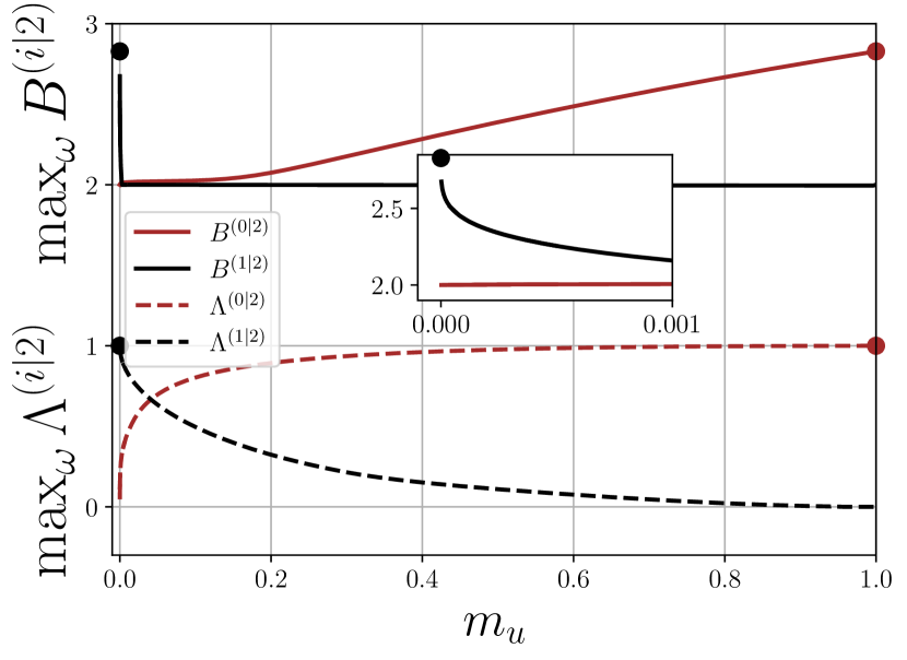
Figure 11: Same as Fig. 4 for zero temperature delta peak configurations. The inset is a blow up at low $m_{u}$.

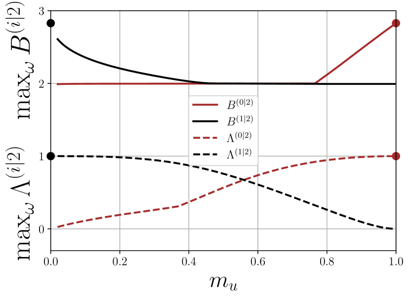
Figure 12: Same as Fig. 4 for zero temperature flat profile configurations with $m_{d}=1/m_{u}^{2}$.

It is in particular of interest to plot the equivalents of Fig. 4 for these alternative configurations. This is done in Figs. 11 and 12. In the flat profile configuration the value of $m_{d}$ is a free parameter. Thus, for comparing the results of the flat profile configuration with Fig. 4 we impose $m_{d}=1/m_{u}^{2}$, as is the case for the waterfall configuration, cf. Eq. (37a). Such a procedure is not required (nor possible) for the delta peak configuration where fixing $m_{u}$ unambiguously determines $m_{d}$, see (37b). Fig. 11 shows that the delta peak configuration has a special feature: the EPR state formed by the companion and the partner (see Sec. III) is only reached at extremely low values of the upstream mach number $m_{u}$, whereas bipartite nonseparability between the Hawking quantum and the partner (modes 0 and 2, respectively) is significant in a wide range of values of $m_{u}$ (roughly speaking, for $m_{u}\gtrsim 0.2$). Despite this peculiarity, it is fair to say that Figs. 11 and 12 both display the same general trend as Fig. 4, supporting the idea that the behavior discussed in the main text is generic. We do not produce finite temperature figures equivalent to Fig. 5 in order not to overload the paper and because, as expected, the delta peak and the flat profile configurations behave similarly to the waterfall configuration when the temperature is increased. There is however a quantitative change which is worth noticing: in these two alternative configurations the violation of bipartite Bell inequality does not persist as much as for the waterfall configuration when $T$ is increased.

It is also quite interesting to study genuine tripartite nonlocality in the delta peak and flat profile configurations by computing the zero temperature value of the Svetlichny parameter $S^{(0|1|2)}(\omega)$ and by then presenting the equivalents of Fig. 6.

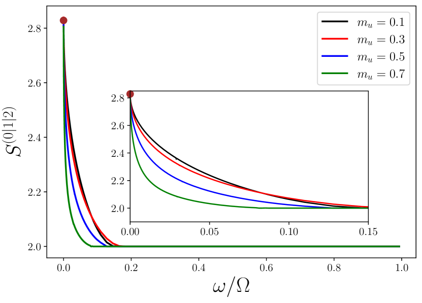
Figure 13: Same as Fig. 6 for zero temperature delta peak configurations. The inset displays a blow up of the figure at low energy.

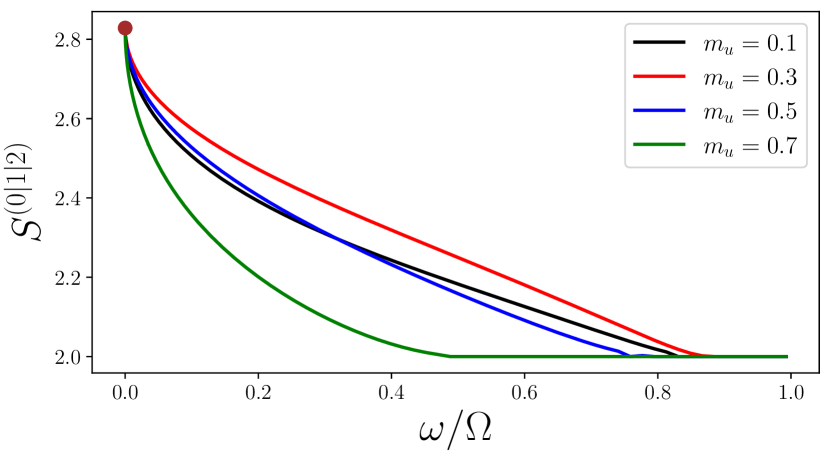
Figure 14: Same as Fig. 6 for zero temperature flat profile configurations.

This is done in Figs. 13 and 14. Here again, the phenomenology is the same as the one discussed in the main text: There is a clear signal of nonlocality at $T=0$, in a domain of energy typically more extended than for the waterfall configuration, but as is the case for the waterfall configuration this signal does not persist at small finite temperature (the corresponding plots are not shown in order not to overload the paper).

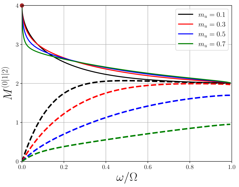
Figure 15: Same as Fig. 8 for delta peak configurations at $T=0$ (thin solid lines) and $T=0.1gn_{u}$ (thick dashed lines).

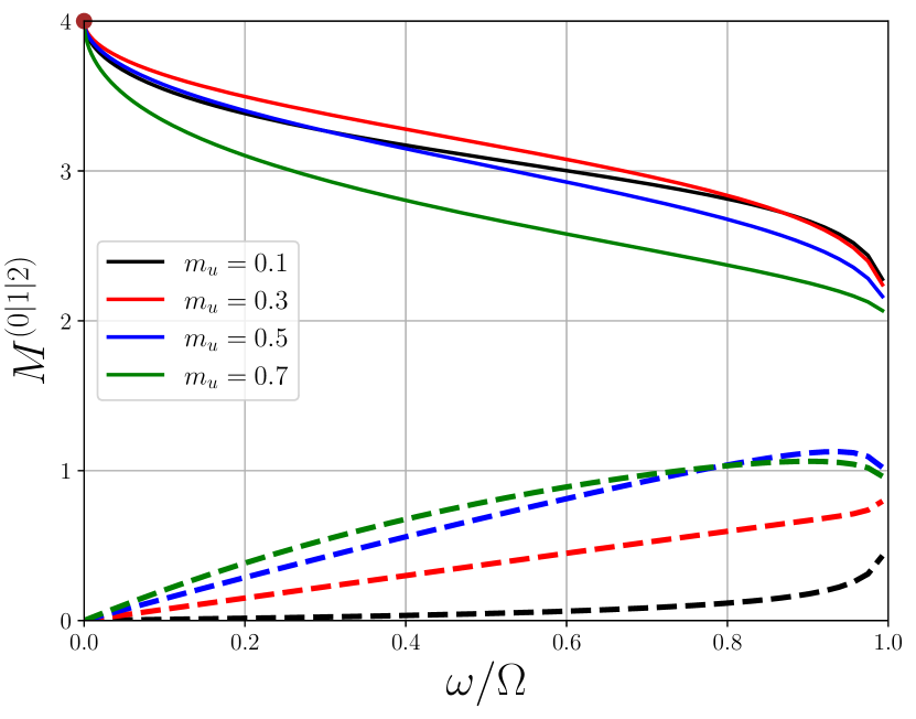
Figure 16: Same as Fig. 8 for flat profile configurations at $T=0$ (thin solid lines) and $T=0.1gn_{u}$ (thick dashed lines).

Finally, it is also important to address the GHZ character of the long wave length modes in the delta peak and flat profile configurations. As argued in Sec. IV of the main text, both configurations display the GHZ paradox at $\omega=0$ and verify $M^{(0|1|2)}(0)=4$ at zero temperature. The behavior of the optimized Mermin parameter $M^{(0|1|2)}(\omega)$ (32) is represented at finite and zero temperature in Figs. 15 and 16 which correspond to the delta peak and flat profile configuration, respectively. At zero temperature the signal (34a) of genuine tripartite entanglement is more pronounced for the delta peak and flat profile configurations that for the waterfall. This was also the case for the signal (34b) of genuine tripartite nonlocality. However, this signal, although more noticeable at $T=0$, is less resilient to an increase of temperature than for the waterfall configuration. The deleterious effect of temperature is particularly pronounced for the flat profile configuration, see Fig. 16. However, although it is clear that each configuration bares its specificities, it is also clear than the general trend is the same: the departure from the GHZ signal $M^{(0|1|2)}(0)=4$ increases at high energy. At finite temperature, the GHZ behavior is lost. The Mermin parameter nonetheless provides a signal of nonlocality if larger than 2. For that matter, the signal is more pronounced at $T\neq 0$ for the waterfall configuration than for the two others.

References

- Penrose and Floyd [1971] R. Penrose and R. M. Floyd, Extraction of rotational energy from a black hole, Nature Physical Science 229, 177 (1971).
- Zel’dovich [1971] Y. B. Zel’dovich, Generation of waves by a rotating body, JETP Lett. 14, 180 (1971).
- Zel’dovich [1972] Y. B. Zel’dovich, Amplification of cylindrical electromagnetic waves reflected from a rotating body, Sov. Phys. JETP 36, 1085 (1972).
- Hawking [1974] S. W. Hawking, Black hole explosions?, Nature (London) 248, 30 (1974).
- Unruh [1981] W. G. Unruh, Experimental black-hole evaporation?, Phys. Rev. Lett. 46, 1351 (1981).
- Weinfurtner et al. [2011] S. Weinfurtner, E. W. Tedford, M. C. J. Penrice, W. G. Unruh, and G. A. Lawrence, Measurement of stimulated Hawking emission in an analogue system, Phys. Rev. Lett. 106, 021302 (2011).
- Euvé et al. [2016] L.-P. Euvé, F. Michel, R. Parentani, T. G. Philbin, and G. Rousseaux, Observation of noise correlated by the Hawking effect in a water tank, Phys. Rev. Lett. 117, 121301 (2016).
- Torres et al. [2017] T. Torres, S. Patrick, A. Coutant, M. Richartz, E. W. Tedford, and S. Weinfurtner, Rotational superradiant scattering in a vortex flow, Nat. Phys. 13, 833 (2017).
- Euvé et al. [2020] L.-P. Euvé, S. Robertson, N. James, A. Fabbri, and G. Rousseaux, Scattering of co-current surface waves on an analogue black hole, Phys. Rev. Lett. 124, 141101 (2020).
- Torres et al. [2020] T. Torres, S. Patrick, M. Richartz, and S. Weinfurtner, Quasinormal mode oscillations in an analogue black hole experiment, Phys. Rev. Lett. 125, 011301 (2020).
- Cromb et al. [2020] M. Cromb, G. M. Gibson, E. Toninelli, M. J. Padgett, E. M. Wright, and D. Faccio, Amplification of waves from a rotating body, Nat. Phys. 16, 1069 (2020).
- Drori et al. [2019] J. Drori, Y. Rosenberg, D. Bermudez, Y. Silberberg, and U. Leonhardt, Observation of stimulated Hawking radiation in an optical analogue, Phys. Rev. Lett. 122, 010404 (2019).
- Braidotti et al. [2022] M. C. Braidotti, R. Prizia, C. Maitland, F. Marino, A. Prain, I. Starshynov, N. Westerberg, E. M. Wright, and D. Faccio, Measurement of Penrose superradiance in a photon superfluid, Phys. Rev. Lett. 128, 013901 (2022).
- Nguyen et al. [2015] H. S. Nguyen, D. Gerace, I. Carusotto, D. Sanvitto, E. Galopin, A. Lemaître, I. Sagnes, J. Bloch, and A. Amo, Acoustic black hole in a stationary hydrodynamic flow of microcavity polaritons, Phys. Rev. Lett. 114, 036402 (2015).
- Jacquet et al. [2020] M. J. Jacquet, T. Boulier, F. Claude, A. Maître, E. Cancellieri, C. Adrados, A. Amo, S. Pigeon, Q. Glorieux, A. Bramati, and E. Giacobino, Polariton fluids for analogue gravity physics, Phil. Trans. R. Soc. A 378, 20190225 (2020).
- Falque et al. [2023] K. Falque, Q. Glorieux, E. Giacobino, A. Bramati, and M. J. Jacquet, Spectroscopic measurement of the excitation spectrum on effectively curved spacetimes in a polaritonic fluid of light (2023), arXiv:2311.01392 [cond-mat.quant-gas] .
- Lahav et al. [2010] O. Lahav, A. Itah, A. Blumkin, C. Gordon, S. Rinott, A. Zayats, and J. Steinhauer, Realization of a sonic black hole analog in a Bose-Einstein condensate, Phys. Rev. Lett. 105, 240401 (2010).
- de Nova et al. [2019] J. R. M. de Nova, K. Golubkov, V. I. Kolobov, and J. Steinhauer, Observation of thermal Hawking radiation and its temperature in an analogue black hole, Nature (London) 569, 688 (2019).
- Kolobov et al. [2021] V. I. Kolobov, K. Golubkov, J. R. Muñoz de Nova, and J. Steinhauer, Observation of stationary spontaneous Hawking radiation and the time evolution of an analogue black hole, Nat. Phys. 17, 362 (2021).
- Isoard et al. [2021] M. Isoard, N. Milazzo, N. Pavloff, and O. Giraud, Bipartite and tripartite entanglement in a Bose-Einstein acoustic black hole, Phys. Rev. A 104, 063302 (2021).
- Brunner et al. [2014] N. Brunner, D. Cavalcanti, S. Pironio, V. Scarani, and S. Wehner, Bell nonlocality, Rev. Mod. Phys. 86, 419 (2014).
- Schmied et al. [2016] R. Schmied, J.-D. Bancal, B. Allard, M. Fadel, V. Scarani, P. Treutlein, and N. Sangouard, Bell correlations in a Bose-Einstein condensate, Science 352, 441 (2016).
- Fadel et al. [2018] M. Fadel, T. Zibold, B. Décamps, and P. Treutlein, Spatial entanglement patterns and Einstein-Podolsky-Rosen steering in Bose-Einstein condensates, Science 360, 409 (2018).
- Kunkel et al. [2018] P. Kunkel, M. Prüfer, H. Strobel, D. Linnemann, A. Frölian, T. Gasenzer, M. Gärttner, and M. K. Oberthaler, Spatially distributed multipartite entanglement enables EPR steering of atomic clouds, Science 360, 413 (2018).
- Colciaghi et al. [2023] P. Colciaghi, Y. Li, P. Treutlein, and T. Zibold, Einstein-Podolsky-Rosen experiment with two Bose-Einstein condensates, Phys. Rev. X 13, 021031 (2023).
- Piano and Adesso [2013] S. Piano and G. Adesso, Genuine tripartite entanglement and nonlocality in Bose-Einstein condensates by collective atomic recoil, Entropy 15, 1875 (2013).
- Lewis-Swan and Kheruntsyan [2015] R. J. Lewis-Swan and K. V. Kheruntsyan, Proposal for a motional-state Bell inequality test with ultracold atoms, Phys. Rev. A 91, 052114 (2015).
- Thomas et al. [2022] K. F. Thomas, B. M. Henson, Y. Wang, R. J. Lewis-Swan, K. V. Kheruntsyan, S. S. Hodgman, and A. G. Truscott, A matter-wave Rarity–Tapster interferometer to demonstrate non-locality, Eur. Phys. J. D 76, 244 (2022).
- Menotti and Stringari [2002] C. Menotti and S. Stringari, Collective oscillations of a one-dimensional trapped Bose-Einstein gas, Phys. Rev. A 66, 043610 (2002).
- Fabbri and Pavloff [2018] A. Fabbri and N. Pavloff, Momentum correlations as signature of sonic Hawking radiation in Bose-Einstein condensates, SciPost Phys. 4, 019 (2018).
- Steinhauer [2016] J. Steinhauer, Observation of quantum Hawking radiation and its entanglement in an analogue black hole, Nat. Phys. 12, 959 (2016).
- Bogoliubov [1947] N. Bogoliubov, On the theory of superfluidity, J. Phys. (USSR) 11, 23 (1947).
- Blaizot and Ripka [1986] J.-P. Blaizot and G. Ripka, Quantum Theory of Finite Systems (MIT Press, Cambridge, Mass, 1986).
- Agullo et al. [2022] I. Agullo, A. J. Brady, and D. Kranas, Quantum aspects of stimulated Hawking radiation in an optical analog white-black hole pair, Phys. Rev. Lett. 128, 091301 (2022).
- Brady et al. [2022] A. J. Brady, I. Agullo, and D. Kranas, Symplectic circuits, entanglement, and stimulated Hawking radiation in analogue gravity, Phys. Rev. D 106, 105021 (2022).
- Macher and Parentani [2009] J. Macher and R. Parentani, Black-hole radiation in Bose-Einstein condensates, Phys. Rev. A 80, 043601 (2009).
- Recati et al. [2009] A. Recati, N. Pavloff, and I. Carusotto, Bogoliubov theory of acoustic Hawking radiation in Bose-Einstein condensates, Phys. Rev. A 80, 043603 (2009).
- de Nova et al. [2014] J. R. M. de Nova, F. Sols, and I. Zapata, Violation of Cauchy-Schwarz inequalities by spontaneous Hawking radiation in resonant boson structures, Phys. Rev. A 89, 043808 (2014).
- Busch and Parentani [2014] X. Busch and R. Parentani, Quantum entanglement in analogue Hawking radiation: When is the final state nonseparable?, Phys. Rev. D 89, 105024 (2014).
- Boiron et al. [2015] D. Boiron, A. Fabbri, P.-E. Larré, N. Pavloff, C. I. Westbrook, and P. Ziń, Quantum signature of analog Hawking radiation in momentum space, Phys. Rev. Lett. 115, 025301 (2015).
- de Nova et al. [2015] J. R. M. de Nova, F. Sols, and I. Zapata, Entanglement and violation of classical inequalities in the Hawking radiation of flowing atom condensates, New J. Phys. 17, 105003 (2015).
- Steinhauer [2015] J. Steinhauer, Measuring the entanglement of analogue Hawking radiation by the density-density correlation function, Phys. Rev. D 92, 024043 (2015).
- Coutant and Weinfurtner [2018] A. Coutant and S. Weinfurtner, Low-frequency analogue Hawking radiation: The Bogoliubov-de Gennes model, Phys. Rev. D 97, 025006 (2018).
- Finazzi and Carusotto [2014] S. Finazzi and I. Carusotto, Entangled phonons in atomic Bose-Einstein condensates, Phys. Rev. A 90, 033607 (2014).
- Robertson et al. [2017] S. Robertson, F. Michel, and R. Parentani, Assessing degrees of entanglement of phonon states in atomic Bose gases through the measurement of commuting observables, Phys. Rev. D 96, 045012 (2017).
- Horstmann et al. [2011] B. Horstmann, R. Schützhold, B. Reznik, S. Fagnocchi, and J. I. Cirac, Hawking radiation on an ion ring in the quantum regime, New J. Phys. 13, 045008 (2011).
- Jacquet and Koenig [2020] M. J. Jacquet and F. Koenig, The influence of spacetime curvature on quantum emission in optical analogues to gravity, SciPost Phys. Core 3, 5 (2020).
- Agullo et al. [2023] I. Agullo, A. J. Brady, and D. Kranas, Robustness of entanglement in Hawking radiation for optical systems immersed in thermal baths, Phys. Rev. D 107, 085009 (2023).
- Delhom et al. [2023] A. Delhom, K. Guerrero, P. Calizaya, K. Falque, A. J. Brady, I. Agullo, and M. J. Jacquet, Entanglement from superradiance and rotating quantum fluids of light (2023), arXiv:2310.16031 [gr-qc] .
- Giovanazzi [2011] S. Giovanazzi, Entanglement entropy and mutual information production rates in acoustic black holes, Phys. Rev. Lett. 106, 011302 (2011).
- Bruschi et al. [2013] D. E. Bruschi, N. Friis, I. Fuentes, and S. Weinfurtner, On the robustness of entanglement in analogue gravity systems, New J. Phys. 15, 113016 (2013).
- Isoard and Pavloff [2020] M. Isoard and N. Pavloff, Departing from thermality of analogue Hawking radiation in a Bose-Einstein condensate, Phys. Rev. Lett. 124, 060401 (2020).
- Isoard [2020] M. Isoard, Theoretical study of quantum correlations and nonlinear fluctuations in quantum gases, Ph.D. thesis, Université Paris-Saclay (2020).
- Leonhardt and Vaccaro [1995] U. Leonhardt and J. A. Vaccaro, Bell correlations in phase space: application to quantum optics, J. Mod. Opt. 42, 939 (1995).
- Gilchrist et al. [1998] A. Gilchrist, P. Deuar, and M. D. Reid, Contradiction of quantum mechanics with local hidden variables for quadrature phase amplitude measurements, Phys. Rev. Lett. 80, 3169 (1998).
- Auberson et al. [2002] G. Auberson, G. Mahoux, S. Roy, and V. Singh, Bell inequalities in phase space and their violation in quantum mechanics, Phys. Lett. A 300, 327 (2002).
- Wenger et al. [2003] J. Wenger, M. Hafezi, F. Grosshans, R. Tualle-Brouri, and P. Grangier, Maximal violation of Bell inequalities using continuous-variable measurements, Phys. Rev. A 67, 012105 (2003).
- García-Patrón et al. [2004] R. García-Patrón, J. Fiurášek, N. J. Cerf, J. Wenger, R. Tualle-Brouri, and P. Grangier, Proposal for a loophole-free Bell test using homodyne detection, Phys. Rev. Lett. 93, 130409 (2004).
- Martin and Vennin [2017] J. Martin and V. Vennin, Obstructions to Bell CMB experiments, Phys. Rev. D 96, 063501 (2017).
- Fine [1982] A. Fine, Hidden variables, joint probability, and the Bell inequalities, Phys. Rev. Lett. 48, 291 (1982).
- Abramsky and Brandenburger [2011] S. Abramsky and A. Brandenburger, The sheaf-theoretic structure of non-locality and contextuality, New J. Phys. 13, 113036 (2011).
- Cavalcanti et al. [2007] E. G. Cavalcanti, C. J. Foster, M. D. Reid, and P. D. Drummond, Bell inequalities for continuous-variable correlations, Phys. Rev. Lett. 99, 210405 (2007).
- Barbosa et al. [2022] R. S. Barbosa, T. Douce, P.-E. Emeriau, E. Kashefi, and S. Mansfield, Continuous-variable nonlocality and contextuality, Commun. Math. Phys. 391, 1047 (2022).
- Gour et al. [2004] G. Gour, F. Khanna, A. Mann, and M. Revzen, Optimization of Bell’s inequality violation for continuous variable systems, Phys. Lett. A 324, 415 (2004).
- Xiang et al. [2017] Y. Xiang, B. Xu, L. Mišta, T. Tufarelli, Q. He, and G. Adesso, Investigating Einstein-Podolsky-Rosen steering of continuous-variable bipartite states by non-Gaussian pseudospin measurements, Phys. Rev. A 96, 042326 (2017).
- Chatterjee and Majumdar [2022] R. Chatterjee and A. S. Majumdar, Bell-inequality violation by dynamical Casimir photons in a superconducting microwave circuit, Phys. Rev. A 106, 042224 (2022).
- Banaszek and Wódkiewicz [1999a] K. Banaszek and K. Wódkiewicz, Testing quantum nonlocality in phase space, Phys. Rev. Lett. 82, 2009 (1999a).
- Chen et al. [2002] Z.-B. Chen, J.-W. Pan, G. Hou, and Y.-D. Zhang, Maximal violation of Bell’s inequalities for continuous variable systems, Phys. Rev. Lett. 88, 040406 (2002).
- Clauser et al. [1969] J. F. Clauser, M. A. Horne, A. Shimony, and R. A. Holt, Proposed experiment to test local hidden-variable theories, Phys. Rev. Lett. 23, 880 (1969).
- [70] From local realism is follows that the measurement of an observable of the type is the product of the result of measurement of the pseudo-spin along direction with the result of measurement of the pseudo-spin along direction , where is the hidden variable. Within this approach, there are only two possible cases: either and are equal (their difference cancels and they sum to ) either they are opposite (their sum cancels and their difference is ). From expression (18) directly follows that such a measurement of yields a result .
- Cirel’son [1980] B. Cirel’son, Quantum generalizations of Bell’s inequality, Lett. Math. Phys. 4, 93–100 (1980).
- Larré et al. [2012] P.-E. Larré, A. Recati, I. Carusotto, and N. Pavloff, Quantum fluctuations around black hole horizons in Bose-Einstein condensates, Phys. Rev. A 85, 013621 (2012).
- Banaszek and Wódkiewicz [1999b] K. Banaszek and K. Wódkiewicz, Nonlocality of the Einstein-Podolsky-Rosen state in the phase space, Acta Phys. Slov. 49, 491 (1999b).
- Svetlichny [1987] G. Svetlichny, Distinguishing three-body from two-body nonseparability by a Bell-type inequality, Phys. Rev. D 35, 3066 (1987).
- Bancal et al. [2011] J.-D. Bancal, N. Brunner, N. Gisin, and Y.-C. Liang, Detecting genuine multipartite quantum nonlocality: A simple approach and generalization to arbitrary dimensions, Phys. Rev. Lett. 106, 020405 (2011).
- Collins et al. [2002] D. Collins, N. Gisin, S. Popescu, D. Roberts, and V. Scarani, Bell-type inequalities to detect true -body nonseparability, Phys. Rev. Lett. 88, 170405 (2002).
- Mermin [1990a] N. D. Mermin, Quantum mysteries revisited, Am. J. Phys. 58, 731 (1990a).
- Coffman et al. [2000] V. Coffman, J. Kundu, and W. K. Wootters, Distributed entanglement, Phys. Rev. A 61, 052306 (2000).
- Dür et al. [2000] W. Dür, G. Vidal, and J. I. Cirac, Three qubits can be entangled in two inequivalent ways, Phys. Rev. A 62, 062314 (2000).
- Adesso et al. [2006] G. Adesso, A. Serafini, and F. Illuminati, Multipartite entanglement in three-mode Gaussian states of continuous-variable systems: Quantification, sharing structure, and decoherence, Phys. Rev. A 73, 032345 (2006).
- Mermin [1990b] N. D. Mermin, Extreme quantum entanglement in a superposition of macroscopically distinct states, Phys. Rev. Lett. 65, 1838 (1990b).
- Klyshko [1993] D. Klyshko, The Bell and GHZ theorems: a possible three-photon interference experiment and the question of nonlocality, Phys. Lett. A 172, 399 (1993).
- Robertson et al. [2018] S. Robertson, F. Michel, and R. Parentani, Nonlinearities induced by parametric resonance in effectively 1D atomic Bose condensates, Phys. Rev. D 98, 056003 (2018).
- Chatrchyan et al. [2021] A. Chatrchyan, K. T. Geier, M. K. Oberthaler, J. Berges, and P. Hauke, Analog cosmological reheating in an ultracold Bose gas, Phys. Rev. A 104, 023302 (2021).
- Butera and Carusotto [2023] S. Butera and I. Carusotto, Numerical studies of back reaction effects in an analog model of cosmological preheating, Phys. Rev. Lett. 130, 241501 (2023).
- de Nova and Sols [2023] J. R. M. de Nova and F. Sols, Black-hole laser to Bogoliubov-Cherenkov-Landau crossover: From nonlinear to linear quantum amplification, Phys. Rev. Res. 5, 043282 (2023).
- Jacobson [1991] T. Jacobson, Black-hole evaporation and ultrashort distances, Phys. Rev. D 44, 1731 (1991).
- Unruh [1995] W. G. Unruh, Sonic analogue of black holes and the effects of high frequencies on black hole evaporation, Phys. Rev. D 51, 2827 (1995).
- Corley and Jacobson [1996] S. Corley and T. Jacobson, Hawking spectrum and high frequency dispersion, Phys. Rev. D 54, 1568 (1996).
- Corley [1998] S. Corley, Computing the spectrum of black hole radiation in the presence of high frequency dispersion: An analytical approach, Phys. Rev. D 57, 6280 (1998).
- Carusotto et al. [2008] I. Carusotto, S. Fagnocchi, A. Recati, R. Balbinot, and A. Fabbri, Numerical observation of Hawking radiation from acoustic black holes in atomic Bose-Einstein condensates, New J. Phys. 10, 103001 (2008).
- Duan et al. [2000] L.-M. Duan, G. Giedke, J. I. Cirac, and P. Zoller, Inseparability criterion for continuous variable systems, Phys. Rev. Lett. 84, 2722 (2000).
- Simon [2000] R. Simon, Peres-Horodecki separability criterion for continuous variable systems, Phys. Rev. Lett. 84, 2726 (2000).
- Williamson [1936] J. Williamson, On the algebraic problem concerning the normal forms of linear dynamical systems, Amer. J. Math. 58, 141 (1936).
- Peres [1996] A. Peres, Separability criterion for density matrices, Phys. Rev. Lett. 77, 1413 (1996).
- Horodecki et al. [1996] M. Horodecki, P. Horodecki, and R. Horodecki, Separability of mixed states: necessary and sufficient conditions, Phys. Lett. A 223, 1 (1996).
- Bennett et al. [1996] C. H. Bennett, D. P. DiVincenzo, J. A. Smolin, and W. K. Wootters, Mixed-state entanglement and quantum error correction, Phys. Rev. A 54, 3824 (1996).
- Adesso and Illuminati [2006] G. Adesso and F. Illuminati, Continuous variable tangle, monogamy inequality, and entanglement sharing in Gaussian states of continuous variable systems, New J. Phys. 8, 15 (2006).
- Adesso and Fuentes-Schuller [2009] G. Adesso and I. Fuentes-Schuller, Correlation loss and multipartite entanglement across a black hole horizon, Quantum Info. Comput. 9, 657–665 (2009).
- Serafini et al. [2005] A. Serafini, G. Adesso, and F. Illuminati, Unitarily localizable entanglement of Gaussian states, Phys. Rev. A 71, 032349 (2005).
- Weedbrook et al. [2012] C. Weedbrook, S. Pirandola, R. García-Patrón, N. J. Cerf, T. C. Ralph, J. H. Shapiro, and S. Lloyd, Gaussian quantum information, Rev. Mod. Phys. 84, 621 (2012).
- Bell [1986] J. S. Bell, EPR correlations and EPW distributions, Ann. N.Y. Acad. Sci. 480, 263 (1986).
- Johansen [1997] L. M. Johansen, EPR correlations and EPW distributions revisited, Phys. Lett. A 236, 173 (1997).
- Banaszek and Wódkiewicz [1998] K. Banaszek and K. Wódkiewicz, Nonlocality of the Einstein-Podolsky-Rosen state in the Wigner representation, Phys. Rev. A 58, 4345 (1998).
- Revzen et al. [2005] M. Revzen, P. A. Mello, A. Mann, and L. M. Johansen, Bell’s inequality violation with non-negative Wigner functions, Phys. Rev. A 71, 022103 (2005).
- [106] The -modes are related to the -modes by a Bogoliubov transformation, see (5). In this case the covariance matrix of the -modes relates to the one of the -modes by a symplectic transform which conserves the determinant (see, e.g., [20] and references therein). At the -modes are all empty and their covariance matrix is the identity . It thus follows that in this case .
- Popescu and Rohrlich [1992] S. Popescu and D. Rohrlich, Generic quantum nonlocality, Phys. Lett. A 166, 293 (1992).
- Horodecki et al. [1995] R. Horodecki, P. Horodecki, and M. Horodecki, Violating Bell inequality by mixed spin- states: necessary and sufficient condition, Phys. Lett. A 200, 340 (1995).
- De Jong et al. [1997] K. De Jong, D. Fogel, and H.-P. Schwefel, Handbook of Evolutionary Computation, edited by T. Baeck, D. B. Fogel, and Z. Michalewicz (CRC Press, 1997) Chap. A2.3. A history of evolutionary computation.
- Beyer and Schwefel [2002] H.-G. Beyer and H.-P. Schwefel, Evolution strategies - a comprehensive introduction, Natural Computing 1, 3 (2002).