T-Explainer: A Model-Agnostic Explainability Framework Based on Gradients

Abstract

The development of machine learning applications has increased significantly in recent years, motivated by the remarkable ability of learning-powered systems to discover and generalize intricate patterns hidden in massive datasets. Modern learning models, while powerful, often exhibit a level of complexity that renders them opaque black boxes, resulting in a notable lack of transparency that hinders our ability to decipher their decision-making processes. Opacity challenges the interpretability and practical application of machine learning, especially in critical domains where understanding the underlying reasons is essential for informed decision-making. Explainable Artificial Intelligence (XAI) rises to meet that challenge, unraveling the complexity of black boxes by providing elucidating explanations. Among the various XAI approaches, feature attribution/importance XAI stands out for its capacity to delineate the significance of input features in the prediction process. However, most existing attribution methods have limitations, such as instability, when divergent explanations may result from similar or even the same instance. In this work, we introduce T-Explainer, a novel local additive attribution explainer based on Taylor expansion endowed with desirable properties, such as local accuracy and consistency, while stable over multiple runs. We demonstrate T-Explainer’s effectiveness through benchmark experiments with well-known attribution methods. In addition, T-Explainer is developed as a comprehensive XAI framework comprising quantitative metrics to assess and visualize attribution explanations.

Keywords: Black-box models, explainable artificial intelligence, XAI, interpretability, local explanations.

1 Introduction

Artificial Intelligence is not a vision for the future. It is our present reality. Terms such as Neural Networks, Machine Learning, Deep Learning, and other facets of the Artificial Intelligence universe have seamlessly shifted from futuristic concepts to near-ubiquitous elements in our daily discourse. The confluence of recent strides in hardware processing capabilities, abundant data accessibility, and refined optimization algorithms has facilitated the creation of intricate and non-linear machine learning models [15]. In the contemporary landscape, those models have achieved unprecedented performance levels, surpassing what was deemed inconceivable just a few years ago, outperforming human abilities and previously known methods in central research areas [67, 63, 56].

The complex non-linear structures and vast number of parameters inherent in such models pose a challenge to transparent interpretation and comprehension of the rationale behind their decisions. Such characteristic transforms those models into black boxes, wherein one can discern only what inputs are provided and what outputs are produced without a clear understanding of the internal decision-making processes [16]. The absence of transparency gives rise to trust-related apprehensions, hindering the effective deployment of potent machine-learning models in critical applications [2, 61, 7]. Additionally, it poses challenges in adhering to emerging regulatory norms observed in numerous countries [25, 57], thereby complicating compliance efforts.

Widely used machine learning models are impenetrable as far as simple interpretations of their mechanisms go [16]. In this context, Explainable Artificial Intelligence (XAI) has emerged to address the challenges outlined above, seeking to provide human-understandable insights into the complexities of models that are inherently challenging to interpret. Significantly, the field of explainability has progressed with the introduction of innovative methodologies, and research focused on discerning the strengths and limitations of XAI models [2]. Feature attribution/importance methods [60] are of particular relevance, aiming to quantify the contribution of individual input variables on predictions made by black-box models [2].

While feature attribution methods prove valuable, they come with drawbacks that diminish the trust and confidence placed in their application. For instance, different methods can result in distinct explanations for the same data instances, making it difficult to decide which outcome to believe [33, 60]. Moreover, many well-known methods, including SHAP [40] and LIME [48], suffer from instability, producing different explanations from different runs on a fixed machine learning model and dataset [23].

To be considered stable, an explanation method must produce consistent explanations in multiple runs on the same and similar instances. Stability is a fundamental objective in XAI, as explainability methods that generate inconsistent explanations for similar instances (or even for the same instance) are challenging to trust. If explanations lack reliability, they become essentially useless. Therefore, to be considered reliable, an explanation model must, at a minimum, exhibit stability [6].

In this work, we introduce T-Explainer, a novel post-hoc explanation method that relies on the solid mathematical foundations of Taylor expansion to perform local and model-agnostic feature importance attributions. T-Explainer is a local additive explanation technique with desirable properties such as local accuracy, missingness, and consistency [40]. Furthermore, T-Explainer is entirely deterministic, guaranteeing stable results across multiple runs and delivering consistent explanations for similar instances.

To evaluate the quality and usefulness of the T-Explainer, we performed several quantitative comparisons against well-known local feature attribution methods, assessing the stability and additivity preservation of such XAI methods. We implemented the T-Explainer integrated with the visualization tools available in the SHAP library, incorporating a suite of quantitative metrics to evaluate feature importance explanations, rendering the T-Explainer a comprehensive XAI framework. In summary, the main contributions of this work are:

• T-Explainer, a stable model-agnostic local additive attribution method derived from the solid mathematical foundation of Taylor expansions. It faithfully approximates the local behavior of black-box models using a deterministic optimization procedure, enabling reliable and trustworthy interpretations.

• A comprehensive set of comparisons against well-known local feature attribution methods using quantitative metrics, aiming mainly to assess stability and additivity preservation.

• A Python library that integrates T-Explainer with other explanation tools, making the proposed method easy to use in different applications. The framework, datasets, and all related materials are openly available online.

2 Related work

Several XAI techniques have been proposed to deal with black-box models. To contextualize our contributions, we focus the following discussion on post-hoc feature importance/attribution methods [18, 68, 33]. A more comprehensive discussion about XAI can be found in several surveys summarizing existing approaches and their properties [2, 7, 38, 12, 17] and metrics for evaluating explanation methods [70, 43, 65, 4].

Breiman [16] proposed one of the first approaches to identify the features most impacting a model prediction. Breiman’s solution is model-specific (Random Forests) and involves permuting the values of each feature and computing the model loss. Given the feature independence assumption, the method identifies the most important features by prioritizing those that contribute the most to the overall loss.

More general approaches, the so-called model-agnostic techniques, can (theoretically) operate with any machine learning model, regardless of the underlying algorithm or architecture. In this context, LIME (Local Interpretable Model-agnostic Explanations) [48], SHAP (SHapley Additive exPlanations) [40], and their variants [47, 49, 22] are model-agnostic methods widely employed to explain machine learning models’ behavior in healthcare [24], financial market [27], and engineering [34] applications.

Although broadly used, LIME and SHAP have significant drawbacks that demand care when using such techniques. For instance, LIME lacks theoretical guarantees about generating accurate simplified approximations for complex models [2]. Moreover, different simplified models can be fit depending on the random sampling mechanism used by LIME, which can lead to instability to small data perturbation and, sometimes, entirely different explanations by just running the code multiple times [13, 6].

SHAP has a solid theoretical foundation derived from game theory [52] that grants SHAP desirable properties such as local accuracy, missingness, and consistency [40]. However, the exact computation of SHAP values is NP-hard, demanding Monte Carlo sampling-based approximations [60], which introduces instability similar to the LIME method, even in its model-specific variants [41, 19, 20]. To avoid instability, deterministic versions of LIME [71], optimization [35], and learning-based [55] approaches have been proposed, but with the price of increasing the number of parameters to be tuned.

Gradient-based methods are another important family of explanation approaches. Those methods attribute importance to each input feature by analyzing how their changes affect the model’s output, relying on gradient decomposition to quantify those effects. Vanilla Gradient [54] introduced the use of gradients to feature attribution tasks. The method computes partial derivatives at the input point $\mathbf{x}$ with a Taylor expansion around a different point $\mathbf{x}^{\prime}$ and a remainder bias term, for which neither is defined [8]. Monte Carlo sampling can be used to estimate derivatives, but it makes Vanilla Gradient suffer from instability and noise within the gradients.

LRP (Layer-wise Relevance Propagation) [8] identifies properties related to the maximum uncertainty state of predictions by redistributing an importance score back to the model’s input layer [36, 28]. The Integrated Gradients method [53] quantifies the feature importance by integrating gradients from the target input to a baseline instance. Input $\times$ Gradient [59] highlights influential regions in the input space by computing the features’ element-wise product and corresponding gradients from the model’s output. DeepLIFT (Deep Learning Important FeaTures) [53] is based on LRP’s importance scores to measure the difference between the model’s prediction of a target input and baseline instance.

The stability of gradient-based methods depends on factors such as the gradient propagation, the model’s complexity, and the baseline choice [53]. Additionally, most of those methods are designed specifically for explanation tasks in Neural Networks and other models with differentiable parameters, which impairs their application to classifiers such as Random Forests and SVMs.

T-Explainer differs from the methods described above in three main aspects: (i) it is deterministic, T-Explainer defines an optimization procedure based on finite differences to estimate partial derivatives, thus being stable by definition; (ii) T-Explainer relies on just a few hyperparameters, rendering it easy to use; and (iii) T-Explainer is not dependent on baselines. Moreover, the T-Explainer is built upon the solid mathematical foundations of Taylor expansion, which naturally endows it with desirable properties similar to those in SHAP. Although T-Explainer, in theory, is designed to be applied to differentiable models, we show experimentally that it also produces interesting results operating with non-differentiable models, which makes T-Explainer more flexible than previous gradient-based methods.

3 The T-Explainer

In this Section, we introduce the theoretical foundations, properties, and computational aspects of the proposed T-Explainer method.

Let $\mathbf{X}$ be a multidimensional dataset where each data instance $\mathbf{x}=(x_{1},\dots,x_{n})\in\mathbf{X}$ is a vector in $\mathbb{R}^{n}$ and $f$ be a machine learning model. For simplicity, let’s assume that $f$ is a binary classification model trained on $\mathbf{X}$, that is, $f(\mathbf{x})\in[0,1]$ accounts for the probability of $\mathbf{x}$ belonging to class $1$, and $(1-f(\mathbf{x}))$ is the probability of belonging to class $0$. All the following reasoning can be extended to regression models.

The model $f$ can be seen as a real-valued function:

$$f:\mathbf{X}\rightarrow[0,1]\subset{\rm I\!R}$$ (1)

As a real function, $f$ can be linearly approximated through first-order Taylor’s expansion:

$$f(\mathbf{x}+\mathbf{h})\approx f(\mathbf{x})+\nabla f(\mathbf{x})\cdot\mathbf{h}$$ (2)

where $\mathbf{h}$ is a displacement vector corresponding to a small neighborhood perturbation of $\mathbf{x}$ and $\nabla f(\mathbf{x})$ is the gradient (linear transformation) of $f$ in $\mathbf{x}$, given by:

$${\nabla}f(\mathbf{x})=\left[{\frac{\partial f(\mathbf{x})}{\partial x_{1}}},\dots,{\frac{\partial f(\mathbf{x})}{\partial x_{n}}}\right].$$ (3)

The $i$-th gradient element corresponds to the partial derivative of $f$ concerning the $i$-th attribute of $\mathbf{x}$. Note that the gradient of $f$ at $\mathbf{x}$ corresponds to the Jacobian matrix when $f$ is a real-valued function. The dot product between the gradient and the displacement vector $\mathbf{h}$ is a linear map from $\mathbb{R}^{n}$ to $\mathbb{R}$, being well-known as the best linear approximation of $f$ in a small neighborhood of $\mathbf{x}$ [44, 45]. Therefore, the gradient can be used to analyze how small perturbations in the input data affect the model output. The right side of Equation 2 is a linear equation that approximates the behavior of $f$ nearby $\mathbf{x}$, and by being a linear mapping, it is naturally interpretable. In other words, the gradient of a model $f$ can be used to generate explanations.

The formulation above resembles the Vanilla Gradient [54] Taylor expansion-based procedure to compute saliency maps. The difference is that, in our case, the attributions are not dependent on class information and do not rely on further parameters specific to the model’s architecture. In addition, T-Explainer differs from previous gradient-based methods by relying on additive explanation modeling and a deterministic optimization procedure to approximate gradients, as described below.

Let $\mathbf{h}=\mathbf{z}^{\prime}\in\mathbb{R}^{n}$ be a perturbation in $\mathbf{x}$, that is, $\mathbf{x}^{\prime}=\mathbf{x}+\mathbf{z}^{\prime}$ is a point in a small neighborhood of $\mathbf{x}$. The T-Explainer can thus be defined as an additive explanation modeling $g_{\mathbf{x}}$, given by:

$$g_{\mathbf{x}}(\mathbf{z}^{\prime})=\phi_{0}+\sum_{i=1}^{n}{\phi_{i}{z}^{\prime}_{i}}$$ (4)

where $\phi_{0}=\mathrm{\mathbb{E}}[f(\mathbf{X})]$ represents the expected prediction value, and $\phi_{i}=\frac{\partial{f}(\mathbf{x})}{\partial x_{i}}$. The prediction expected value is a statistical value that is not trivial to estimate for an arbitrary dataset. In practice, it is computed through the average model output across the training dataset $\mathbf{X}$ when the feature values $\mathbf{X}_{i}$ are unknown. As a fundamental property of additive explanations, Equation 4 approximates the original predicted value $f(\mathbf{x})$ locally by summing its feature importances [40].

The explanation model $g_{\mathbf{x}}$ is a local attribution method, i.e., there is a $g_{\mathbf{x}}$ for each $\mathbf{x}$. By definition, the T-Explainer is an additive feature attribution method, as defined by Lundberg and Lee [40], meaning that the importance value attributed to each feature can reconstruct the model prediction by summating those importance values. The coefficient $\phi_{i}$ indicates the feature attribution/importance of the $i$-th attribute to the prediction made by $f$ in $\mathbf{x}$. In T-Explainer, the feature attribution $\phi_{i}$ has a simple and intuitive geometric interpretation, corresponding to the projection of $\nabla f(\mathbf{x})$ on the $i$-th feature axis. Therefore, the more aligned the gradient $\nabla f(\mathbf{x})$ and the $i$-th axis of the feature space, the more important the $i$-th feature is to the decision made by $f$.

3.1 T-Explainer Properties

According to Lundberg and Lee [40], a “good” explanation method must hold three important properties, namely, Local Accuracy, Missingness, and Consistency. In the following, we show that the T-Explainer approximates Local Accuracy while holding Missingness and Consistency.

3.1.1 Local Accuracy

The local accuracy property, as defined by Lundberg and Lee [40], states that if $f(\mathbf{x}+\mathbf{z}^{\prime})=g_{\mathbf{x}}(\mathbf{z}^{\prime})=\phi_{0}+\sum_{i=1}^{n}{\phi_{i}{z}^{\prime}_{i}}$, then $g_{\mathbf{x}}$ holds the local accuracy property. The T-Explainer does not exactly satisfy this property but rather approximates it. By construction, we have:

$$f(\mathbf{x}+\mathbf{z}^{\prime})\approx g_{\mathbf{x}}(\mathbf{z}^{\prime})=\phi_{0}+\sum_{i=1}^{n}{\phi_{i}{z}^{\prime}_{i}}$$ (5)

and, from the Taylor expansion remainder theorem [42], there is an upper-bound to the approximation error given by:

$${f(\mathbf{x}+\mathbf{z}^{\prime})-g_{\mathbf{x}}(\mathbf{z}^{\prime})=O({\|\mathbf{z}^{\prime}\|}^{2})}.$$ (6)

3.1.2 Missingness

The missingness property states that if a feature $x_{i}$ has no impact on the model decision, then $\phi_{i}=0$ (see [40, 58]). In our context, a feature $i$ having no impact in $f$ means that $f$ does not vary (increase or decrease) when only such $i$-th feature is changed (otherwise, the feature would impact the model decision). In other words, $f(x_{1},\dots,x_{i}+{z}^{\prime}_{i},\dots,x_{n})-f(x_{1},\dots,x_{i},\dots,x_{n})=0$, thus, there is no variation in the $i$-th direction and the partial derivative $\phi_{i}=\frac{\partial f(\mathbf{x})}{\partial x_{i}}=0$, ensuring that the T-Explainer holds the missingness property.

3.1.3 Consistency

Let $f$ and $\tilde{f}$ be two binary classification models. Let’s use the notation $\mathbf{x}^{\prime}\backslash i$ to indicate that the $i$-th feature is disregarded in any perturbation of $\mathbf{x}$ (${z}^{\prime}_{i}=0$ in any perturbation, so ${x}^{\prime}_{i}\backslash i=x_{i}$). An explanation method is consistent if (see Lundberg and Lee [40]), fixing $\mathbf{x}$, $\tilde{f}(\mathbf{x}^{\prime})-\tilde{f}(\mathbf{x}^{\prime}\backslash i)>f(\mathbf{x}^{\prime})-f(\mathbf{x}^{\prime}\backslash i)$ implies $\phi_{i}(\tilde{f})>\phi_{i}(f)$.

Suppose that $\tilde{f}(\mathbf{x}^{\prime})-\tilde{f}(\mathbf{x}^{\prime}\backslash i)>f(\mathbf{x}^{\prime})-f(\mathbf{x}^{\prime}\backslash i)$ holds in a small neighborhood of $\mathbf{x}$, in particular,

$$\tilde{f}(x_{1}+{z}^{\prime}_{1},\dots,x_{i} +{z}^{\prime}_{i},\dots,x_{n}+{z}^{\prime}_{n})-$$

$$\tilde{f}(x_{1}+{z}^{\prime}_{1},\dots,x_{i},\dots,x_{n}+{z}^{\prime}_{n})>$$ (7)

$$f(x_{1}+{z}^{\prime}_{1},\dots, x_{i}+{z}^{\prime}_{i},\dots,x_{n}+{z}^{\prime}_{n})-$$

$$f(x_{1}+{z}^{\prime}_{1},\dots,x_{i},\dots,x_{n}+{z}^{\prime}_{n})$$

for ${z}^{\prime}_{i}\in(-\delta,0)\cup(0,\delta)$.

Define $\tilde{s}({z}^{\prime}_{i})=\frac{\tilde{f}(\mathbf{x}^{\prime})-\tilde{f}(\mathbf{x}^{\prime}\backslash i)}{{z}^{\prime}_{i}}$ and ${s}({z}^{\prime}_{i})=\frac{{f}(\mathbf{x}^{\prime})-{f}(\mathbf{x}^{\prime}\backslash i)}{{z}^{\prime}_{i}}$, from Equation 3.1.3 we know that $\tilde{s}({z}^{\prime}_{i})>{s}({z}^{\prime}_{i})$ for ${z}^{\prime}_{i}\in(-\delta,0)\cup(0,\delta)$. Assuming that $\tilde{f}$ and ${f}$ are differentiable in $\mathbf{x}$, then $\lim_{{z}^{\prime}_{i}\to 0}\tilde{s}({z}^{\prime}_{i})=\frac{\partial\tilde{f}(\mathbf{x})}{\partial x_{i}}$ and $\lim_{{z}^{\prime}_{i}\to 0}{s}({z}^{\prime}_{i})=\frac{\partial{f}(\mathbf{x})}{\partial x_{i}}$ exist, thus, from the Limit Inequality Theorem:

$$\phi_{i}(\tilde{f})=\frac{\partial\tilde{f}(\mathbf{x})}{\partial x_{i}}>\frac{\partial{f}(\mathbf{x})}{\partial x_{i}}=\phi_{i}({f})$$ (8)

showing that the T-Explainer holds the consistency property (the Limit Inequality Theorem ensures that, given two functions $\tilde{s},s:(a,c)\cup(c,b)\subset{\rm I\!R}\rightarrow{\rm I\!R}$, if $\tilde{s}(x)>s(x)$ for all $x\in(a,c)\cup(c,b)$ and the limits $\lim_{x\to c}\tilde{s}(x)=A$ and $\lim_{x\to c}{s}(x)=B$ exist, then $A>B$).

According to Lundberg and Lee [40], the Shapley-based explanation is the unique possible additive feature attribution model that (theoretically, see Hooker et al. [31]) satisfies Local Accuracy, Missingness, and Consistency properties. As demonstrated above, the T-Explainer approximates Local Accuracy while holding Missingness and Consistency. Therefore, the T-Explainer is one of the few XAI methods that get close to SHAP regarding theoretical guarantees.

3.2 T-Explainer: Computational Aspects

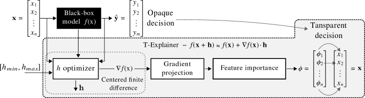
Figure 1: T-Explainer pipeline.

Figure 1 illustrates the step-by-step pipeline of T-Explainer for feature attribution. Computing the gradient of a known real-valued function is (theoretically) simple, demanding to take the partial derivatives of the function. However, we need to calculate partial derivatives of an arbitrary black-box model $f$, which was previously trained and holds complex internal mechanisms. To that end, we perturb the instance $\mathbf{x}$ attribute-wise and compute the respective change in the model’s output, approximating the partial derivatives through centered finite differences [37]:

$$FD_{f(\mathbf{x})}=\frac{f(\mathbf{x}+\mathbf{h})-f(\mathbf{x}-\mathbf{h})}{2\mathbf{h}}.$$ (9)

Finite differences are well-established approaches to approximate differential equations, replacing the derivatives with discrete approximations (such transformation results in computationally feasible systems of equations) [37].

Specifically, we rely on the centered finite difference because that approach simply averages two one-sided perturbations of each attribute, resulting in a second-order accurate approximation with an error proportional to $\mathbf{h}^{2}$ [37]. The centered finite difference approximation of the partial derivatives demands to set up the magnitude of the perturbation $\mathbf{h}$. The displacement $\mathbf{h}$ must be small enough to generate a perturbation close to the input data $\mathbf{x}$. By definition, the derivatives of $f$ are computed by making $\mathbf{h}\to 0$ in Equation 9. In other words, we have to set $\mathbf{h}$ to a small value.

In practice, if $\mathbf{h}$ is too small, it can generate significant round-off errors or singularity cases. On the other hand, if $\mathbf{h}$ is too large, it can lead to truncation errors and inappropriate approximations. As far as we know, there is no closed solution to determine an optimum value to $\mathbf{h}$. To solve this issue, we developed a $\mathbf{h}$ optimizer method based on a binary search that minimizes a mean squared error (MSE) cost function. The method runs over the $[h_{min},h_{max}]$ interval, searching for an optimal $\mathbf{h}$ to produce a good approximation of $f(\mathbf{x})$ from Equation 2. We set $h_{min}$ with the minimum distance between any two instances on the dataset, i.e., $h_{min}=\min_{i,j=1}^{n}||{\mathbf{x}_{i}}-{\mathbf{x}_{j}}||$, $\forall{i}\neq{j},\mathbf{x}_{i},\,\mathbf{x}_{j}\in\mathbf{X}$. The optimization method is formulated as follows:

$$\nabla f(\mathbf{x})=\underset{\mathbf{h}\in[h_{min},h_{max}]}{\mathrm{arg\,min}}\ \mathcal{L}(f,\mathbf{h},\epsilon_{\mathbf{x}})+\theta(\nabla f_{\mathbf{x}})$$ (10)

where $\mathcal{L}$ is the cost function (MSE in our case), $\nabla f_{\mathbf{x}}$ represents the approximated value of the gradient $\nabla f(\mathbf{x})$ in each iteration of the $\mathbf{h}$ optimizer algorithm computing the method in Equation 9 on Equation 2, $\epsilon_{\mathbf{x}}$ is the cost threshold upper-bounded by $h_{min}^{2}$ [37], and $\theta$ is a method that ensures the numerical stability of the optimization process by checking if $\mathbf{h}$ is keeping the gradient (Jacobian matrix) $\nabla f_{\mathbf{x}}$ non-singular (or full-rank). It is important to highlight that local perturbations must preserve the data’s normalization range to avoid model extrapolations [31]. Further details about the optimization process are given in the Appendix Section. This approach can find the gradient ${\nabla f(\mathbf{x})}$ of a binary-class model or even the entire Jacobian related to all the model’s output probabilities. Once the gradient is estimated in $\mathbf{x}$, the importance of each attribute is computed as $\phi_{i}=\frac{\partial{f}(\mathbf{x})}{\partial x_{i}}$.

The explanations must remain consistent with the model’s behavior in the instance’s locality to ensure meaningful interpretability. Through the $\mathbf{h}$ optimization process, T-Explainer attributes feature importance using Taylor’s expansion for each instance tailored to its local characteristics. In other words, the T-Explainer is primarily designed as a local explainer. According to Ribeiro et al. [48], simultaneously achieving local and global fidelity in XAI is challenging because aggregating local explanations to estimate global feature importance might be ineffective due to local explanations being instance-specific and often inconsistent with global explanations. However, the adaptive $\mathbf{h}$ optimization strategy of T-Explainer is flexible enough to be extended and generate aggregated views while preserving local relationships, enhancing consistent and interpretable explanations locally and also at global levels.

3.2.1 Handling Categorical Data

All the considerations outlined above assume the attributes are continuous numerical data. However, most datasets are not limited to numerical data but also encompass categorical (nominal or qualitative) features. Handling categorical data is challenging, as many learning models cannot directly process nominal features, demanding numerical conversions. Different approaches can be applied to encode categorical values as numerical representations, including the well-known one-hot encoding [50].

Numerical encodings introduce challenges for XAI methods, particularly for the gradient-based ones. Nominal values represented with one-hot encode become binary constant values (zeros and ones), thus being discontinuous attributes where partial derivatives can not be properly estimated, inducing the explainer to erroneously attribute null importance to features that may significantly impact the prediction.

T-Explainer has a modular design that enhances flexible additions or improvements of functionalities. To address the challenges of categorical features, we implemented a mechanism to handle one-hot encoded columns into the T-Explainer framework. Once the user identifies the one-hot encoded categorical attributes, a procedure transforms them into intervals through continuous perturbations. Specifically, the $0$ and $1$ values (resulting from one-hot encoding) are uniformly perturbed with displacement in the interval $\delta\in(-0.5,0.5)$, creating a range of values around $0$ and $1$, simulating a continuous set of values around these two values.

The continuity induction procedure is performed over a copy of the training dataset, with the perturbed columns being normalized to the same interval of the numerical features (typically in the $[0,1]$ range). After that, transfer learning is applied in a copy of the original model, fitting it with the perturbed training dataset (the categorical fitted model). Finally, the T-Explainer runs on the newly trained model. In summary, predictions of instances holding categorical features are explained using the T-Explainer’s core implementation. However, we incorporated a preliminary layer in T-Explainer’s pipeline to handle categorical data.

The perturbation radius $\delta$ can impact the accuracy of the categorical fitted model, making it disagree with the original model. However, the disagreement varies depending on the training data. In our experiments, the proposed transformation of categorical attributes to numerical ones does not significantly impact the accuracy of the categorical fitted model for perturbations into small intervals. We fixed $\delta=0.1$ as the perturbation radius, which ensured the accuracy preservation.

4 Quantitative Metrics

In this Section, we describe the evaluation metrics integrated into the T-Explainer framework. Relative Input Stability (RIS) and Relative Output Stability (ROS) [3, 4] are metrics used to evaluate the stability of local explanations to changes in input data and output prediction probabilities, respectively. We followed the basic definitions in Agarwal et al. [3] but introduced improvements to address the issues described below.

Given $\mathcal{N}_{\mathbf{x}}$ a neighborhood of perturbed instances $\mathbf{x}^{\prime}$ around $\mathbf{x}$, with $e_{\mathbf{x}}$ and $e_{\mathbf{x}^{\prime}}$ representing the attribution vectors explaining $\mathbf{x}$ and $\mathbf{x}^{\prime}$, and $f({\mathbf{x}})$ and $f({\mathbf{x}^{\prime}})$ the output prediction probabilities of $\mathbf{x}$ and $\mathbf{x}^{\prime}$, RIS and ROS metrics are formally defined as:

$$\text{RIS}(\mathbf{x},\mathbf{x}^{\prime},e_{\mathbf{x}},e_{\mathbf{x}^{\prime}})=\max_{\mathbf{x}^{\prime}}{\frac{\|\frac{e_{\mathbf{x}}-e_{\mathbf{x}^{\prime}}}{e_{\mathbf{x}}}\|_{p}}{\max{(\|\frac{\mathbf{x}-\mathbf{x}^{\prime}}{\mathbf{x}}\|_{p},\epsilon_{c})}}}\>\>\>\>\text{and}$$ (11)

$$\text{ROS}(\mathbf{x},\mathbf{x}^{\prime},e_{\mathbf{x}},e_{\mathbf{x}^{\prime}})=\max_{\mathbf{x}^{\prime}}{\frac{\|\frac{e_{\mathbf{x}}-e_{\mathbf{x}^{\prime}}}{e_{\mathbf{x}}}\|_{p}}{\max{(\|\frac{f(\mathbf{x})-f(\mathbf{x}^{\prime})}{f(\mathbf{x})}\|_{p},\epsilon_{c})}}}$$ (12)

$\forall\mathbf{x}^{\prime}\in\mathcal{N}_{\mathbf{x}}$, with ${p}$ defining the $l_{p}$ norm used to measure the changes and $\epsilon_{c}>0$ as a clipping threshold to avoid zero division. The larger the RIS or ROS values, the more unstable the method is related to input or output prediction perturbation.

RIS and ROS handle values close to zero in the normalization processes. However, the original metrics implemented in Agarwal et al. [4] applied a clip method that ignores significant negative values by handling any negative value as a small value. Then, we designed a clip method that preserves significant values, both positive and negative, while discarding those close to zero. The original implementations may also ignore instances near the model’s decision boundaries. We solved that issue by sampling perturbations of each $\mathbf{x}$, sorting the perturbed data based on the distance to $\mathbf{x}$, and generating a neighborhood holding a minimum set of perturbed instances. This way, we ensure coverage and avoid measurement omissions or potential crashes in the metrics. Additionally, we extended RIS and ROS to evaluate the mean changes and the respective standard deviations, in addition to the original maximum change in explanations.

A novel metric, Run Explanation Stability (RES), was added to our framework to measure the local stability through multiple runs on non-perturbed inputs. RES assesses the consistency of several explanations for the same instance under the same settings, with higher values indicating lower stability rates. Given $n$ explanations $g_{\mathbf{x}i},\dots,g_{\mathbf{x}n}$ of the same instance $\mathbf{x}$, with each $g_{\mathbf{x}i}$ as a scalar representing the prediction approximation (see Equation 4), let $\bar{g}_{\mathbf{x}}$ be the mean explanation from those $n$ explanations. We define the RES metric as:

$$\text{RES}(g_{\mathbf{x}},\bar{g}_{\mathbf{x}})=\max_{k=1}^{n}{\|\bar{g}_{\mathbf{x}}-g_{\mathbf{x}k}\|}\text{,}\>\>\>\forall\mathbf{x}\in\mathbf{X}\text{.}$$ (13)

The Reiteration Similarity metric inspired the rationale behind RES [6]; however, we simplified the formulation using standard deviation as the similarity measure.

Another new addition is the Faithfulness of an Additive Explanator (FAE) metric, which assesses how an additive feature importance explainer preserves the primary property of local accuracy, i.e., the model prediction should be reconstructed by the summation of the importance values as in Equation Equation 5 [40]. Given an output prediction probability $f(\mathbf{x})$ and its explanation $g_{\mathbf{x}}$, we define the FAE metric as the frequency or ratio in which $\|f(\mathbf{x})-g_{\mathbf{x}}\|\geq\epsilon$, $\forall\mathbf{x}\in\mathbf{X}$, with $\epsilon$ a tolerance threshold. Aiming to analyze better each model’s additiveness, the FAE metric also computes the mean values in which $\|f(\mathbf{x})-g_{\mathbf{x}}\|$. In this case, the smaller the FAE mean, the closer the approximations between $f(\mathbf{x})$ and $g_{\mathbf{x}}$ will be from the threshold $\epsilon$ and, thus, the more “additive” the model is (the explainer is more faithful regarding the local accuracy property).

RIS, ROS, RES, and FAE metrics are unitless quantifiers with no “ideal” desirable values. Reasonable values depend on the context of the application, meaning those metrics must be interpreted relatively by comparing their results across XAI methods [5].

5 Experiments

This section presents the configurations and outcomes of the experiments undertaken to evaluate T-Explainer, employing a diverse set of datasets, models, and comparison metrics. In all experiments described below, we are evaluating local explanation tasks.

5.1 Experimental Setup

We trained Multi-Layer Perceptions (MLP) Neural Networks from scikit-learn (https://scikit-learn.org/) and Gradient-boosted Tree Ensemble classifiers (Random Forests-based) from the XGBoost gradient boosting library [21] as the black-box models used throughout the experiments. Logistic Regressions and SVMs could also be viable alternatives, but we focused on Neural Networks and Random Forests due to their wide adoption in Machine Learning. The models were trained with a dataset split of $80\%$ for training and $20\%$ for testing. Such division was achieved using the $train\_test\_split$ method from scikit-learn, with a consistent shuffling seed across all datasets. We conducted a Grid Search to determine the hyperparameters that optimize the models’ performance.

For the MLPs, we initialized the hyperparameters search using powers of $2$ for the number of neurons in the hidden layers, following standard practices in this context [60]. We employed the ReLU activation function, Stochastic Gradient Descent as the optimizer and the log-loss function. We evaluated alternative activation functions and optimizers, but they did not yield gains. The Tree Ensemble model’s hyperparameters were defined by specifying ranges for the number of decision tree estimators and the maximum depth of each estimator, utilizing cross-entropy loss as the evaluation metric for classification.

We selected three different MLP models from the hyperparameters tunning: a three and a five hidden layers neural network holding $64$ neuron units per layer (3H-NN and 5H-64-NN, respectively) and a five-layer neural network with $[64,128,128,128,64]$ neurons in each layer (5H-128-NN). All the neural network models use a learning rate of $0.01$, alpha $0.0001$, and maximum training epochs of $500$. The selected neural networks achieved better performances considering our classification tasks. We based our architectures on previous works [9, 15], with extra neural units and additional layers significantly increasing the training time without noticeably increasing performance.

Following our hyperparameters tunning, the Tree Ensemble classifiers (XRFC) have $500$ estimators, a maximum depth of $6$, a learning rate of $0.01$, and a gamma equal to $1$. All the other hyperparameters are the libraries’ default for Neural Networks and Tree Ensembles. Those models are used as the base black boxes for comparing T-Explainer against SHAP [40], LIME [48], and three Gradient-based methods [32] such as Integrated Gradients, Input $\times$ Gradient, and DeepLIFT. Specifically, we used the SHAP explainer for neural networks and the TreeSHAP explainer [41] for tree-based classifiers. Although SHAP, LIME, and Gradient-based methods were proposed a few years back, we benchmark T-Explainer with them because they continue to be the most widely used feature attribution explainers in research and practice [4].

For each experiment requiring data perturbation, we used the NormalPerturbation method from OpenXAI [4] to generate perturbed neighborhoods with $\mu=0$, $\sigma^{2}=0.001$, a flip percentage $\varepsilon_{p}=0.0001$, and the perturbation maximum distance of $h_{min}/2$, ensuring neighborhoods with small perturbations around each instance. We also specified the clipping threshold to handle values close to zero as $\epsilon_{c}=\pm{10^{-5}}$ and the $l_{p}$ norm as the Euclidean ($p=2$).

To avoid round-off issues and enhance readability, we use scientific notation to represent values larger than ${10}^{5}$, while values smaller than ${10}^{-10}$ will be taken as zero.

5.2 Synthetic Data

We generate two different synthetic datasets comprising $1000$ instances each. The first is a 4-dimensional (4-FT) dataset where each instance $\mathbf{x}$ is generated as follows. We distribute the target label $\mathbf{y}\in[0,1]$ equally across each dataset half; thus, each class has $500$ instances. Conditioned to the value of $\mathbf{y}$, we sample the instance $\mathbf{x}$ as $x_{1:2}\sim\mathcal{N}(\mu_{y},\,\Sigma_{y})$. We choose $\mu_{0}=[0,0]^{\mathrm{T}}$ and $\mu_{1}=[-2,2]^{\mathrm{T}}$, $\Sigma_{0}=[[1,1],[-1,1]]^{\mathrm{T}}$ and $\Sigma_{1}=\mathbf{I}$, where $\mu_{0}$, $\Sigma_{0}$ and $\mu_{1}$, $\Sigma_{1}$ denote the means and covariance matrices of the Gaussian distributions associated with instances in classes $0$ and $1$ respectively. The features $x_{1:2}$ are called $core\_1$ and $core\_2$. Random values are assigned to the features $x_{3:4}$ ($noise\_1$ and $noise\_2$). Such configuration results in a dataset holding two predictive (important) and two random noise (non-important) features with a small mixture area between the important features to introduce a degree of complexity to the predictive process.

The second synthetic dataset is more robust. It is a 20-dimensional (20-FT) dataset created using the OpenXAI synthetic data generation tool, whose algorithm is described in Agarwal et al. [4]. According to the authors, the algorithm ensures the creation of a dataset that encapsulates feature dependencies and clear local neighborhoods, key properties to guarantee the explanations derived from this synthetic dataset remain consistent with the behavior of the models trained on such data.

We used the XRFC and 3H-NN models over the synthetic datasets experiments. The XRFC classifier achieved $96\%$ accuracy on the 4-FT data and $83.5\%$ accuracy on the 20-FT synthetic dataset, while the 3H-NN model achieved $97.5\%$ accuracy on the 4-FT data and $83.5\%$ accuracy on the 20-FT dataset. Note that we are not basing our benchmark experiments on synthetic datasets with massive amounts of instances. We know it is necessary to use a reasonable amount of data to train and test machine learning models. According to Aas et al. [1], well-known feature importance methods become unstable in tasks with more than ten dimensions. In this sense, data dimensionality is more critical to assessing the stability of feature importance methods than the number of instances. Thus, we generated synthetic datasets with enough instances ($1000$ for each dataset) to train our models and assess the XAI methods.

Figures 2(a) and 2(b) present explanations generated by TreeSHAP and T-Explainer for the same instance predicted with the XRFC model. As expected, TreeSHAP attributed the most significant importance to feature $core\_1$ (followed by $core\_2$). However, TreeSHAP attributed a negative signal to $core\_1$, pushing the additive reconstruction (see Equation 5) of TreeSHAP to $-0.013$, while the true prediction for this instance is $0.0134$. Thus, the TreeSHAP explanation indicates that the instance belongs to the opposite class, disagreeing with the model prediction (and also the instance label) and violating the Local Accuracy property. T-Explainer also points to $core\_1$ (and $core\_2$) as the most important feature but with a correct positive signal.

Table 1 provides a broad view of the scenario illustrated in Figure 2. We used the FAE metric (considering $0.01$ as the tolerance threshold) to assess Local Accuracy preservation by T-Explainer, SHAP, and TreeSHAP when applied to the XRFC model on the 4-FT dataset. TreeSHAP, the model-specific version of SHAP, presented a faithful additivity rate of $0.507$ of its explanations. T-Explainer preserved the additivity property with a $0.425$ rate, slightly lower than TreeSHAP. However, the T-Explainer was far better than the SHAP model-agnostic version of the SHAP explainer framework. In contrast, Table 2 shows that the T-Explainer outperforms all the other additive methods regarding Local Accuracy preservation on the 20-FT dataset holding a $0.862$ preservation rate.

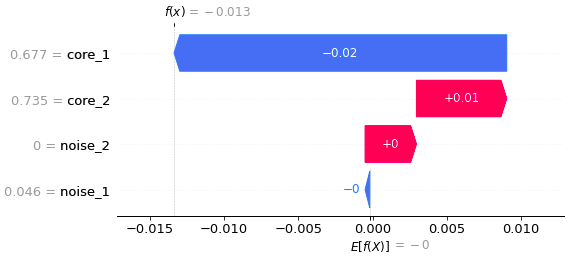
(a) TreeSHAP feature importances.

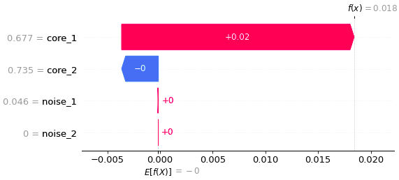
(b) T-Explainer feature importances.

Figure 2: TreeSHAP and T-Explainer importances of the same instance classified with XRFC on the 4-FT dataset.

XRFC	FAE
XAI	Mean	Ratio
T-Explainer	0.0178	0.425
SHAP	0.5072	0.007
TreeSHAP	0.0186	0.507

Table 1: T-Explainer, SHAP, and TreeSHAP Local Accuracy when explaining the XRFC predictions on the 4-FT dataset.

XRFC	FAE
XAI	Mean	Ratio
T-Explainer	0.0053	0.862
SHAP	0.4601	0.319
TreeSHAP	0.0103	0.620

Table 2: T-Explainer, SHAP, and TreeSHAP Local Accuracy when explaining the XRFC predictions on the 20-FT dataset.

Table 3 shows the RIS, ROS, and RES stability metrics for T-Explainer, TreeSHAP, and LIME, explaining the XRFC model on the 4-FT data. Notice that TreeSHAP has the best RIS, ROS, and RES results. The good performance of TreeSHAP is expected, as the 4-FT is a low-dimensional dataset, and TreeSHAP takes advantage of it by relying on a deterministic version of Shapley values computation [6]. Table 4 shows the same metrics for the 3H-NN model on the 4-FT dataset. The T-Explainer performed considerably better than the other XAI methods in terms of RIS ($7\times$ better than DeepLIFT), ROS, and also the RES metric.

XRFC	RIS		ROS		RES
XAI	Max	Mean	Max	Mean	Max
T-Exp	13,819	111.4	6e+06	38,904	0
TreeSHAP	5,053	38.0	5e+05	8,226	0
LIME	10,895	200.4	6e+06	86,050	3e-04

Table 3: Stability of XAI methods explaining the XRFC predictions on the 4-FT synthetic dataset. T-Exp is the T-Explainer, and Max refers to the maximum value.

3H-NN	RIS		ROS		RES
XAI	Max	Mean	Max	Mean	Max
T-Exp	176	5.97	806	5.82	0
SHAP	2,010	38.59	12,122	51.39	0
LIME	4,625	127.1	1.7e+05	296.9	3e-02
I-Grad	2,465	19.33	1,169	7.41	0
I$\times$Grad	1,316	9.75	1,535	7.74	1e-05
DeepLIFT	1,316	9.75	1,535	7.74	1e-05

Table 4: Stability of XAI methods explaining the 3H-NN predictions on the 4-FT dataset. I-Grad and I$\times$Grad are Integrated Gradients and Input $\times$ Gradient, respectively.

Tables 5 and 6 depict the results from the XRFC and 3H-NN models on the 20-FT dataset. From Table 5, we can see that T-Explainer is superior to TreeSHAP and LIME in the RIS and ROS metrics for both maximum and mean values. TreeSHAP reached a close performance regarding maximum ROS, but T-Explainer is considerably better on the average ROS. Similar results can be observed in Table 6, where T-Explainer beat all the other explainers in terms of RIS ($3\times$ better than Integrated Gradients), with slightly better performance than Integrated Gradients in the mean ROS but outperforming all the other explainers in maximum ROS. SHAP was the most unstable method, which can be justified in the context of the 20-FT dataset because, in high-dimensional spaces, SHAP uses a random sampling algorithm rather than the deterministic one, leading to unstable explanations [6]. Moreover, SHAP is also prone to suffer from extrapolations [30, 31].

XRFC	RIS		ROS		RES
XAI	Max	Mean	Max	Mean	Max
T-Exp	728	28.95	2.6e+06	35,596	0
TreeSHAP	897	37.83	3.3e+06	64,204	0
LIME	1,117	143.6	21.6e+06	3.5e+05	1e-04

Table 5: Stability of XAI methods explaining the XRFC predictions on the 20-FT synthetic dataset.

3H-NN	RIS		ROS		RES
XAI	Max	Mean	Max	Mean	Max
T-Exp	717	26.2	17,887	99.98	0
SHAP	2.8e+05	7,272	2e+06	14,076	2e-01
LIME	10,182	125.6	28,063	301.9	3e-02
I-Grad	2,279	28.35	39,287	107.4	0
I$\times$Grad	11,815	63.36	60,787	217.2	5e-06
DeepLIFT	11,813	63.36	60,781	217.2	5e-06

Table 6: Stability of XAI methods explaining the 3H-NN predictions on the 20-FT dataset.

In general, Tables 3, 4, 5, and 6 show that T-Explainer is robust regarding different stability metrics, being among the best performance methods, especially when data dimensionality is high.

The T-Explainer’s performance when dealing with the XRFC model, which is a non-differentiable model, is also remarkable. Therefore, although not theoretically supported, the T-Explainer might perform well even when applied to generate explanations for non-differentiable machine learning models.

5.3 Real Data

This Section extends the evaluations and comparisons by applying real data from different domains. Specifically, we run experiments using four well-known real datasets with distinct properties regarding dimensionality, the presence of categorical attributes, and size.

The Banknote Authentication [39] is a $4$-dimensional dataset containing $1,372$ instances with measurements of genuine and forged banknote specimens. The German Credit [29] comprises $9$ features (numerical and categorical) covering financial, demographic, and personal information from $1,000$ credit applicants, each categorized into good or bad risk.

The Home Equity Line of Credit (HELOC) dataset provided by FICO [26] consists of financial attributes from anonymized applications for home equity lines of credit submitted by $9,871$ real homeowners. The task in the HELOC dataset is to predict whether an applicant has a good or bad risk of repaying their HELOC account within two years. The largest dataset in our study is HIGGS [9], which contains $28$ features about simulated collision events to distinguish between Higgs bosons signals and a background process. The original HIGGS dataset contains $11$ million instances, but we used the $98,050$ instances version available at OpenML [64]. Table 7 summarizes the real datasets.

	Banknote	German	HELOC	HIGGS
#Instances	1,372	1,000	9,871	98,050
#Num features	4	4	21	28
#Cat features	0	5	2	0
#Classes	2	2	2	2

Table 7: Properties of the real datasets. Num features and Cat features refer to numeric and categorical features, respectively.

The experiments with real data have been conducted using only the neural network models, as some of the explanation models with which T-Explainer is compared are specifically designed for neural networks. Moreover, the neural network models are differentiable, thus meeting the theoretical requirements that support the T-Explainer technique. We further discuss tree-based models in Section 7.

For the experiments with Banknote Authentication and German Credit datasets, we selected the 3H-NN model. From Table 8, one can see that T-Explainer is less stable than Integrated Gradients, but it is the second-best method on average for RIS and ROS (closely tied with Integrated Gradients for RES). Table 9 presents the stability tests using the German Credit data. The original version of the dataset has $20$ numerical and categorical attributes. Still, it is practically impossible to directly apply it in a machine learning task due to its complex categorization system.

We pre-processed the German Credit data to clean it, resulting in a reduced version holding nine features ($4$ numerical and $5$ categorical features, see Table 7). As shown in Table 9, T-Explainer performed as the most stable explainer regarding RIS and maximum ROS perturbations, being the second best for the mean ROS.

3H-NN	RIS		ROS		RES
XAI	Max	Mean	Max	Mean	Max
T-Exp	175.29	3.09	429.31	4.05	0
SHAP	1.3e+05	468	1.9e+05	543	0
LIME	97.57	9.34	849.02	13.43	3e-02
I-Grad	12.37	1.54	429.23	2.09	0
I$\times$Grad	175.33	4.41	427.97	4.12	2e-05
DeepLIFT	175.33	4.41	427.97	4.12	2e-05

Table 8: Stability of XAI methods explaining the 3H-NN predictions on the Banknote Authentication dataset.

3H-NN	RIS		ROS		RES
XAI	Max	Mean	Max	Mean	Max
T-Exp	1,971	49.4	15,735	239.9	0
SHAP	1.0e+06	14,044	2.5e+07	62,883	2.1e-01
LIME	7,547	131.1	1.8e+05	739.9	2.4e-02
I-Grad	8,709	59.5	58,721	185.7	0
I$\times$Grad	10,933	63.2	1.0e+05	350.8	2.8e-06
DeepLIFT	10,934	63.2	1.0e+05	350.8	2.4e-06

Table 9: Stability of XAI methods explaining the 3H-NN predictions on the German Credit dataset.

Tables 8 and 9 indicate that gradient-based methods are more stable to input/output perturbations than SHAP and, in some cases, also than LIME. As one can notice, T-Explainer competes quite well with other gradient-based methods.

HELOC and HIGGS are more robust datasets in terms of dimensionality and size. We selected the 3H-NN and the five-layer neural network models to compare T-Explainer with the other explainers on those datasets. Specifically, we trained the 3H-NN and 5H-128-NN classifiers on HELOC, achieving $71.34\%$ and $73.27\%$ accuracy, respectively. Despite the accuracy values being lower than the ones we achieved before, those performances are in line with the results reported in the literature [15].

Table 10 shows that Integrated Gradients is the most stable explainer for almost all metrics (behind LIME only for mean RIS but with very close numbers). However, we highlight the performance of T-Explainer, especially regarding the metrics’ means. Only Integrated Gradients, LIME, and T-Explainer kept the mean RIS under ten units, which can be taken as virtually the same mean stability to input perturbations. Similar results are observed in mean ROS, where Integrated Gradients, LIME, and T-Explainer achieved the smallest values, being T-Explainer the second best. Table 11 shows the explainers’ stability when applied to the five-layer neural network. In such case, T-Explainer is the most stable method, with Integrated Gradients being the second best for mean RIS and LIME as the second best for mean ROS. Only T-Explainer and Integrated Gradients matched RES with the highest levels of stability.

3H-NN	RIS		ROS		RES
XAI	Max	Mean	Max	Mean	Max
T-Exp	1,443	8.49	94,943	527.9	0
SHAP	84,794	1,330	1.7e+07	64,693	1.5e-02
LIME	509.7	3.84	3.7e+05	626.5	9.3e-02
I-Grad	159.8	4.21	85,463	401.1	0
I$\times$Grad	3,754	33.67	3.5e+05	1,879	8.7e-07
DeepLIFT	3,749	33.64	3.5e+05	1,878	9.0e-07

Table 10: Stability of XAI methods explaining the 3H-NN predictions on the HELOC dataset.

5H-128-NN	RIS		ROS		RES
XAI	Max	Mean	Max	Mean	Max
T-Exp	154.0	5.37	1.4e+05	362.5	0
SHAP	52,924	1,757	1.6e+07	67,451	1.9e-01
LIME	5,083	39.96	2.5e+05	935.0	1.6e-02
I-Grad	255.7	7.21	1.9e+07	19,283	0
I$\times$Grad	11,769	66.01	4.3e+05	3,215	1.8e-06
DeepLIFT	11,785	66.06	4.3e+05	3,218	1.7e-06

Table 11: Stability of XAI methods explaining the 5H-128-NN predictions on the HELOC dataset.

We trained the 3H-NN and 5H-64-NN classifiers on the HIGGS data, which achieved $69.58\%$ and $66.83\%$ accuracy, respectively, close to the values reported in previous works [15]. We included a set of benchmarks using a five-layer neural network here to keep some similarity with the architectures proposed in Baldi et al. [9], which explored the use of deep networks on HIGGS. Tables 12 and 13 show the good stability performances of gradient-based feature importance explainers, with T-Explainer outperforming them regarding RIS perturbations while being quite competitive regarding ROS and RES metrics. Those results demonstrate T-Explainer’s ability to generate consistent explanations through different levels of model complexity and data dimensionality. Note that SHAP is more unstable than LIME, with SHAP’s claimed advantageous performance predominantly seen in low-dimensional datasets [6].

3H-NN	RIS		ROS		RES
XAI	Max	Mean	Max	Mean	Max
T-Exp	1,063	45.0	69,645	304.4	0
SHAP	1.4e+05	5,213	8.8e+05	22,190	2.05e-01
LIME	4,424	90.0	69,458	492.6	3.19e-02
I-Grad	3,833	49.7	27,719	272.4	0
I$\times$Grad	2,030	79.9	70,159	604.3	6.62e-06
DeepLIFT	2,031	79.9	70,153	604.3	6.32e-06

Table 12: Stability of XAI methods explaining the 3H-NN predictions on the HIGGS dataset.

5H-64-NN	RIS		ROS		RES
XAI	Max	Mean	Max	Mean	Max
T-Exp	1,359	57.7	65,999	330.4	0
SHAP	1.3e+05	4,309	7.3e+06	19,999	2.22e-01
LIME	9,582	130.8	46,700	477.2	3.50e-02
I-Grad	15,619	101.1	37,091	452.2	0
I$\times$Grad	4,036	123.9	84,022	558.6	1.67e-05
DeepLIFT	4,036	123.9	84,021	558.6	1.69e-05

Table 13: Stability of XAI methods explaining the 5H-64-NN predictions on the HIGGS dataset.

Finally, the experiments above show that T-Explainer generally performs well, clearly outperforming well-known model-agnostic methods such as SHAP (and LIME for most tests). Our method presented competitive results in setups differing from Neural Networks, proving its agnostic capability. Moreover, T-Explainer also turned out to be quite competitive with model-specific techniques such as the gradient-based ones, thus being a new and valuable alternative method to explain black-box models’ predictions.

6 Computational Performance

Another challenge that XAI methods have to face is related to computational performance. Shapley-based approaches like SHAP apply sampling approximations because the exact version of the method is an NP-hard problem with exponential computing time regarding the number of features [40]. SHAP is a leading method in feature attribution tasks due to its axiomatic properties, with a range of explainers based on different algorithms, from the exact version to optimized approaches. However, according to its documentation, the most precise algorithm is only feasible for modelings that are nearly limited to $15$ features.

For a computational comparison of T-Explainer’s performance, we generated a synthetic dataset with $16$ features (16-FT) using OpenXAI, similar to the 20-FT dataset we used before (see the Synthetic Data Section). The 3H-NN model was trained with the 16-FT dataset according to the experimental setup defined in Section 5.1. We then defined ten explanation tasks, increasing the number of explanations by ten instances from the 16-FT data for each task, ranging from ten to one hundred explanations, to compare T-Explainer with three implementations of SHAP – the optimized explainer (the same method used in the stability experiments of Section 5), KernelSHAP [40], the exact explainer based on standard Shapley values computation. Figure 3 presents the computational performance of T-Explainer and SHAP.

Figure 3: Running times of SHAP and T-Explainer applied to the 3H-NN model trained on 16-dimensional synthetic data.

SHAP explainer was the fastest. However, the method was the most unstable, as we demonstrated in the stability assessments. The T-Explainer’s performance is close to KernelSHAP, while the SHAP exact explainer running time has grown exponentially. In such a performance test, we used a reduced dataset instead of the 20-FT data because applying the SHAP exact explainer in tasks with more than $16$ features is impossible. Most of the Machine Learning problems consider high-dimensional data. For example, the HIGGS is a 28-dimensional dataset with over $98$ thousand instances. With that dataset, it is impossible to apply the exact version of SHAP, and the optimized version of SHAP performs very poorly. Something similar could be said about the HELOC data, which recently motivated a challenge by FICO [26]. In this sense, T-Explainer is placed as a competitive XAI approach regarding computational resources.

7 Discussion, Limitations, and Future Work

T-Explainer is backed by a clearly defined deterministic optimization process for calculating partial derivatives. This new approach gives T-Explainer more robustness, as demonstrated in our results.

Our experiments have focused on binary classification models, which are known to perform well in supervised learning [15]. However, there is no constraint in applying T-Explainer to regression problems or more complex models, such as deep learning models. In particular, the T-Explainer naturally supports regression or multi-class classification with minor adaptations, which we are currently working on.

Although T-Explainer has demonstrated competitive results when applied to tree-based models on synthetic data, tree-based architectures impose extra challenges on XAI. Tree classifiers have non-continuous architectures in which constant values are stored in leaf nodes, rendering gradient-based methods inappropriate. T-Explainer’s current version is not yet fully developed to support tree-based models. We are currently designing a mechanism that enables the computation of gradients in tree-based models, extending T-Explainer to operate in a more general context.

The present implementation of the T-Explainer can handle categorical attributes through an approach that discretizes categorical data into intervals, using continuous perturbations, enabling the computation of partial derivatives. However, the approach requires a model retraining to fit the continuous intervals induced in the columns containing one-hot encoded categorical attributes. Retraining introduces additional computational complexity. Getting around the retraining issue is another improvement we are currently working on. One alternative approach we are considering in this context is to apply the target encoding transformer [10], which converts each nominal value of a categorical attribute into its corresponding expected value.

We conducted experiments and comparisons using tabular data to create classification models for simplicity and because it is a typical setup for machine learning problems in academia and industry [15, 69]. We highlight that our experimental setup followed the assessment practices in recent literature [9, 33, 60, 11], focusing on Neural Networks as black boxes [38] and including datasets where leading XAI approaches have stability and applicability difficulties. However, we designed the T-Explainer considering more complex data representations, such as 2D images, videos, or semantic segmentation. We are extending our approach to encompass simplification masking approaches, a strategy widely used by many XAI methods [46, 40].

Another aspect under improvement is the $\mathbf{h}$ optimization module. As far as we know, there is no closed solution to determine an optimum value to $\mathbf{h}$ in this context. During our investigations, we observed that the finite difference computation presents a certain instability for instances near the model’s decision boundaries due to discontinuities imposed by the decision boundaries. The literature on numerical methods brings a number of alternatives to deal with discontinuities when approximating derivatives through finite differences [62, 51]. As part of the T-Explainer’s core, we are investigating alternatives to refine the $\mathbf{h}$ optimization process while maintaining computational efficiency.

A comprehensive assessment of a local explanation technique requires extensive quantitative [14] and qualitative [66] evaluations, including insights from human analysts [70]. We prioritized quantitative metrics in this work, particularly those concerning stability, but we acknowledge the value of humans in the loop assessment. Thus, we are committed to comprehensively validating the T-Explainer using metrics beyond those discussed here.

When carefully developed and applied, explainability contributes by adding new trustworthy perspectives to the broad horizon of Machine Learning, enriching the next generation of transparent Artificial Intelligence applications [36]. As an evolving project, T-Explainer will continue to be expanded and updated, incorporating additional functionalities and refinements. Our goal is to provide a complete XAI suite in Python based on implementations of T-Explainer and its functionalities in a well-documented and user-friendly package.

8 Conclusion

In this paper, we presented the T-Explainer, a Taylor expansion-based XAI technique. T-Explainer is a deterministic local feature attribution method built upon a solid mathematical foundation that grants it relevant properties such as local accuracy, missingness, and consistency. Moreover, T-Explainer is designed to be a model-agnostic method able to generate explanations for a wide range of machine learning models, as it relies only on the models’ outputs without accounting for their internal structure or partial results. The provided experiments and comparisons demonstrate that T-Explainer is quite stable and comparable to model-specific techniques, thus being a valuable explanation alternative.

9 Appendix

Our $\mathbf{h}$ optimizer was designed to find a reasonable estimate of the displacement parameter $\mathbf{h}$ when running the centered finite difference method ($FD$) to compute the partial derivatives required by T-Explainer. The optimizer is based on a binary search that minimizes a mean squared error (MSE) cost function. The optimum $\mathbf{h}$ should be a small enough value but not too small to avoid round-off errors or singularity cases and should not be too large to avoid truncation errors. Algorithm 1 provides high-level details about the optimization process to estimate the $\mathbf{h}$ parameter. If $\mathbf{h}$ leads to a singular or rank-deficient Jacobian matrix, the final ${\nabla}f_{\mathbf{x}}$ will lead T-Explainer to attribute misleading null values to potentially important features. Then, $\theta$ is a function that keeps the numerical stability by checking if the gradient of $f$ comes from a non-singular (or full-rank) matrix.

Algorithm 1 The $\mathbf{h}$ optimizer. The input parameter $max\_itr$ defines the maximum number of iterations.

References

- Aas et al. [2021] Kjersti Aas, Martin Jullum, and Anders Løland. Explaining individual predictions when features are dependent: More accurate approximations to shapley values. Artificial Intelligence, 298:103502, 2021.
- Adadi and Berrada [2018] Amina Adadi and Mohammed Berrada. Peeking inside the black-box: A survey on explainable artificial intelligence (XAI). IEEE Access, 6:52138–52160, 2018.
- Agarwal et al. [2022a] Chirag Agarwal, Nari Johnson, Martin Pawelczyk, Satyapriya Krishna, Eshika Saxena, Marinka Zitnik, and Himabindu Lakkaraju. Rethinking stability for attribution-based explanations. Preprint arXiv:2203.06877, 2022a.
- Agarwal et al. [2022b] Chirag Agarwal, Eshika Saxena, Satyapriya Krishna, Martin Pawelczyk, Nari Johnson, Isha Puri, Marinka Zitnik, and Himabindu Lakkaraju. OpenXAI: Towards a transparent evaluation of model explanations. Preprint arXiv:2206.11104, 2022b.
- Alvarez-Melis and Jaakkola [2018] David Alvarez-Melis and Tommi S Jaakkola. On the robustness of interpretability methods. Preprint arXiv:1806.08049, 2018.
- Amparore et al. [2021] Elvio Amparore, Alan Perotti, and Paolo Bajardi. To trust or not to trust an explanation: using LEAF to evaluate local linear XAI methods. PeerJ Computer Science, 7:e479, 2021.
- Arrieta et al. [2020] Alejandro Barredo Arrieta, Natalia Díaz-Rodríguez, Javier Del Ser, Adrien Bennetot, Siham Tabik, Alberto Barbado, Salvador García, Sergio Gil-López, Daniel Molina, Richard Benjamins, et al. Explainable artificial intelligence (XAI): Concepts, taxonomies, opportunities and challenges toward responsible AI. Information Fusion, 58:82–115, 2020.
- Bach et al. [2015] Sebastian Bach, Alexander Binder, Grégoire Montavon, Frederick Klauschen, Klaus-Robert Müller, and Wojciech Samek. On pixel-wise explanations for non-linear classifier decisions by layer-wise relevance propagation. PLOS One, 10(7):e0130140, 2015.
- Baldi et al. [2014] Pierre Baldi, Peter Sadowski, and Daniel Whiteson. Searching for exotic particles in high-energy physics with deep learning. Nature Communications, 5(1):4308, 2014.
- Banachewicz et al. [2022] Konrad Banachewicz, Luca Massaron, and Anthony Goldbloom. The Kaggle Book: Data analysis and machine learning for competitive data science. Packt Publishing Ltd, Birmingham, UK, 2022.
- Barr et al. [2023] Brian Barr, Noah Fatsi, Leif Hancox-Li, Peter Richter, Daniel Proano, and Caleb Mok. The disagreement problem in faithfulness metrics. In NeurIPS XAI in Action: Past, Present, and Future Applications, pages 1–13, New Orleans, Louisiana, USA, 2023. NeurIPS.
- Belle and Papantonis [2021] Vaishak Belle and Ioannis Papantonis. Principles and practice of explainable machine learning. Frontiers in Big Data, page 39, 2021.
- Bhatt et al. [2020] Umang Bhatt, Alice Xiang, Shubham Sharma, Adrian Weller, Ankur Taly, Yunhan Jia, Joydeep Ghosh, Ruchir Puri, José M. F. Moura, and Peter Eckersley. Explainable machine learning in deployment. In 2020 ACM Conference on Fairness, Accountability, and Transparency, page 648–657, New York, NY, USA, 2020. Association for Computing Machinery.
- Bodria et al. [2021] Francesco Bodria, Fosca Giannotti, Riccardo Guidotti, Francesca Naretto, Dino Pedreschi, and Salvatore Rinzivillo. Benchmarking and survey of explanation methods for black box models. Preprint arXiv:2102.13076, 2021.
- Borisov et al. [2022] Vadim Borisov, Tobias Leemann, Kathrin Seßler, Johannes Haug, Martin Pawelczyk, and Gjergji Kasneci. Deep neural networks and tabular data: A survey. IEEE Transactions on Neural Networks and Learning Systems, 7:1–41, 2022.
- Breiman [2001] Leo Breiman. Random forests. Machine Learning, 45(1):5–32, 2001.
- Burkart and Huber [2021] Nadia Burkart and Marco F Huber. A survey on the explainability of supervised machine learning. Journal of Artificial Intelligence Research, 70:245–317, 2021.
- Casalicchio et al. [2018] Giuseppe Casalicchio, Christoph Molnar, and Bernd Bischl. Visualizing the feature importance for black box models. In Joint European Conference on Machine Learning and Knowledge Discovery in Databases, pages 655–670. Springer, 2018.
- Chen et al. [2021] Hugh Chen, Scott Lundberg, and Su-In Lee. Explaining models by propagating Shapley values of local components. In Explainable AI in Healthcare and Medicine, pages 261–270. Springer, New York City, NY, USA, 2021.
- Chen et al. [2022] Hugh Chen, Scott M Lundberg, and Su-In Lee. Explaining a series of models by propagating Shapley values. Nature Communications, 13(1):1–15, 2022.
- Chen and Guestrin [2016] Tianqi Chen and Carlos Guestrin. XGBoost: A scalable tree boosting system. In Proceedings of the 22nd ACM SIGKDD International Conference on Knowledge Discovery and Data Mining, KDD ’16, page 785–794, New York, NY, USA, 2016. Association for Computing Machinery.
- Covert and Lee [2021] Ian Covert and Su-In Lee. Improving kernelshap: Practical shapley value estimation using linear regression. In Int. Conf. on Artificial Intelligence and Statistics, pages 3457–3465, San Diego, California, USA, 2021. PMLR.
- Dai et al. [2022] Jessica Dai, Sohini Upadhyay, Ulrich Aivodji, Stephen H Bach, and Himabindu Lakkaraju. Fairness via explanation quality: Evaluating disparities in the quality of post hoc explanations. In AAAI/ACM Conference on AI, Ethics, and Society, pages 203–214, 2022.
- Duell et al. [2021] Jamie Duell, Xiuyi Fan, Bruce Burnett, Gert Aarts, and Shang-Ming Zhou. A comparison of explanations given by explainable artificial intelligence methods on analysing electronic health records. In IEEE EMBS Int. Conf. on Biomedical and Health Informatics, pages 1–4. IEEE, 2021.
- EU Regulation [2016] EU Regulation. 2016/679 of the European Parliament and of the council of 27 april 2016 on the General Data Protection Regulation. http://data.europa.eu/eli/reg/2016/679/oj, 2016. Online, visited on April 2023.
- FICO [2019] FICO. Home equity line of credit (HELOC) dataset. https://community.fico.com/s/explainable-machine-learning-challenge, 2019. Accessed: 2023-09-10.
- Gramegna and Giudici [2021] Alex Gramegna and Paolo Giudici. Shap and lime: an evaluation of discriminative power in credit risk. Frontiers in Artificial Intelligence, 4:752558, 2021.
- Hamilton et al. [2021] Mark Hamilton, Scott Lundberg, Lei Zhang, Stephanie Fu, and William T Freeman. Model-agnostic explainability for visual search. Preprint arXiv:2103.00370, 2021.
- Hofmann [1994] Hans Hofmann. Statlog (German Credit Data). UCI Repository. Irvine: University of California, School of Information and Computer Sciences, 1994.
- Hooker and Mentch [2019] Giles Hooker and Lucas Mentch. Please stop permuting features: An explanation and alternatives. Preprint arXiv:1905.03151, 2019.
- Hooker et al. [2021] Giles Hooker, Lucas Mentch, and Siyu Zhou. Unrestricted permutation forces extrapolation: variable importance requires at least one more model, or there is no free variable importance. Statistics and Computing, 31(6):1–16, 2021.
- Kokhlikyan et al. [2020] Narine Kokhlikyan, Vivek Miglani, Miguel Martin, Edward Wang, Bilal Alsallakh, Jonathan Reynolds, Alexander Melnikov, Natalia Kliushkina, Carlos Araya, Siqi Yan, et al. Captum: A unified and generic model interpretability library for PyTorch. Preprint arXiv:2009.07896, 2020.
- Krishna et al. [2022] Satyapriya Krishna, Tessa Han, Alex Gu, Javin Pombra, Shahin Jabbari, Steven Wu, and Himabindu Lakkaraju. The disagreement problem in explainable machine learning: A practitioner’s perspective. Preprint arXiv:2202.01602, 2022.
- Kuzlu et al. [2020] Murat Kuzlu, Umit Cali, Vinayak Sharma, and Özgür Güler. Gaining insight into solar photovoltaic power generation forecasting utilizing explainable artificial intelligence tools. IEEE Access, 8:187814–187823, 2020.
- Lakkaraju et al. [2020] Himabindu Lakkaraju, Nino Arsov, and Osbert Bastani. Robust and stable black box explanations. In International Conference on Machine Learning, pages 5628–5638. PMLR, 2020.
- Lapuschkin et al. [2019] Sebastian Lapuschkin, Stephan Wäldchen, Alexander Binder, Grégoire Montavon, Wojciech Samek, and Klaus-Robert Müller. Unmasking Clever Hans predictors and assessing what machines really learn. Nature Communications, 10(1):1–8, 2019.
- LeVeque [2007] Randall J LeVeque. Finite difference methods for ordinary and partial differential equations: steady-state and time-dependent problems. SIAM, Philadelphia, PA, USA, 2007.
- Linardatos et al. [2020] Pantelis Linardatos, Vasilis Papastefanopoulos, and Sotiris Kotsiantis. Explainable ai: A review of machine learning interpretability methods. Entropy, 23(1):18, 2020.
- Lohweg [2013] Volker Lohweg. Banknote Authentication. UCI Repository. Irvine: University of California, School of Information and Computer Sciences, 2013.
- Lundberg and Lee [2017] Scott M Lundberg and Su-In Lee. A unified approach to interpreting model predictions. In Proceedings of the 31st International Conference on Neural Information Processing Systems, pages 4768–4777, Long Beach, CA, USA, 2017. Curran Associates Inc.
- Lundberg et al. [2018] Scott M Lundberg, Gabriel G Erion, and Su-In Lee. Consistent individualized feature attribution for tree ensembles. Preprint arXiv:1802.03888, 2018.
- Marsden and Tromba [2003] Jerrold E Marsden and Anthony Tromba. Vector calculus. Macmillan, United Kingdom, 2003.
- Mohseni et al. [2021] Sina Mohseni, Niloofar Zarei, and Eric D Ragan. A multidisciplinary survey and framework for design and evaluation of explainable ai systems. ACM Trans. on Int. Intell. Sys., 11(3-4):1–45, 2021.
- Nocedal and Wright [1999] Jorge Nocedal and Stephen J Wright. Numerical optimization. Springer, New York, NY, USA, 1999.
- Press [2007] William H Press. Numerical recipes 3rd edition: The art of scientific computing. Cambridge University Press, Cambridge, UK, 2007.
- Ribeiro et al. [2016a] Marco Tulio Ribeiro, Sameer Singh, and Carlos Guestrin. Model-agnostic interpretability of machine learning. Preprint arXiv:1606.05386, 2016a.
- Ribeiro et al. [2016b] Marco Tulio Ribeiro, Sameer Singh, and Carlos Guestrin. Nothing else matters: model-agnostic explanations by identifying prediction invariance. Preprint arXiv:1611.05817, 2016b.
- Ribeiro et al. [2016c] Marco Tulio Ribeiro, Sameer Singh, and Carlos Guestrin. “Why should I trust you?” Explaining the predictions of any classifier. In Proceedings of the 22nd ACM SIGKDD International Conference on Knowledge Discovery and Data Mining, pages 1135–1144, San Francisco, CA, USA, 2016c. NY ACM.
- Ribeiro et al. [2018] Marco Tulio Ribeiro, Sameer Singh, and Carlos Guestrin. Anchors: High-precision model-agnostic explanations. Proceedings of the AAAI Conference on Artificial Intelligence, 32(1), 2018.
- Rodríguez et al. [2018] Pau Rodríguez, Miguel A. Bautista, Jordi Gonzàlez, and Sergio Escalera. Beyond one-hot encoding: Lower dimensional target embedding. Image and Vision Computing, 75:21–31, 2018.
- Scheinberg [2022] Katya Scheinberg. Finite difference gradient approximation: To randomize or not? INFORMS Journal on Computing, 34(5):2384–2388, 2022.
- Shapley [1953] Lloyd S Shapley. A value for n-person games. In Contributions to the Theory of Games (AM-28), Volume II, page 2, Princeton, New Jersey, USA, 1953. Princeton University Press.
- Shrikumar et al. [2017] Avanti Shrikumar, Peyton Greenside, and Anshul Kundaje. Learning important features through propagating activation differences. In 34th International Conference on Machine Learning, pages 3145–3153, Sydney, Australia, 2017. PMLR.
- Simonyan et al. [2013] Karen Simonyan, Andrea Vedaldi, and Andrew Zisserman. Deep inside convolutional networks: Visualising image classification models and saliency maps. Preprint arXiv:1312.6034, 2013.
- Situ et al. [2021] Xuelin Situ, Ingrid Zukerman, Cecile Paris, Sameen Maruf, and Gholamreza Haffari. Learning to explain: Generating stable explanations fast. In Proceedings of the 59th Annual Meeting of the Association for Computational Linguistics and the 11th International Joint Conference on Natural Language Processing (Volume 1: Long Papers), pages 5340–5355, 2021.
- Snider et al. [2022] Eric J Snider, Sofia I Hernandez-Torres, and Emily N Boice. An image classification deep-learning algorithm for shrapnel detection from ultrasound images. Scientific Reports, 12(1):1–12, 2022.
- State of California [2021] State of California. California consumer privacy act (CCPA). https://oag.ca.gov/privacy/ccpa, 2021. Online, visited on July 2023.
- Sundararajan and Najmi [2020] Mukund Sundararajan and Amir Najmi. The many Shapley values for model explanation. In 37th International Conference on Machine Learning, pages 9269–9278, Vienna, Austria, 2020. PMLR.
- Sundararajan et al. [2017] Mukund Sundararajan, Ankur Taly, and Qiqi Yan. Axiomatic attribution for deep networks. In International Conference on Machine Learning, pages 3319–3328. PMLR, 2017.
- Tan et al. [2023] Sarah Tan, Giles Hooker, Paul Koch, Albert Gordo, and Rich Caruana. Considerations when learning additive explanations for black-box models. Machine Learning, pages 1–27, 2023.
- Tjoa and Guan [2020] Erico Tjoa and Cuntai Guan. A survey on explainable artificial intelligence (XAI): Toward medical XAI. IEEE Transactions on Neural Networks and Learning Systems, 2020.
- Towers [2009] John D Towers. Finite difference methods for approximating heaviside functions. Journal of Computational Physics, 228(9):3478–3489, 2009.
- Ullman [2019] Shimon Ullman. Using neuroscience to develop artificial intelligence. Science, 363(6428):692–693, 2019.
- Vanschoren et al. [2014] Joaquin Vanschoren, Jan N Van Rijn, Bernd Bischl, and Luis Torgo. OpenML: networked science in machine learning. ACM SIGKDD Explorations Newsletter, 15(2):49–60, 2014.
- Vitali [2022] Fabio Vitali. A survey on methods and metrics for the assessment of explainability under the proposed ai act. In Legal Knowledge and Information Systems, volume 346, page 235. IOS Press, 2022.
- Weerts et al. [2019] Hilde JP Weerts, Werner van Ipenburg, and Mykola Pechenizkiy. A human-grounded evaluation of SHAP for alert processing. Preprint arXiv:1907.03324, 2019.
- Wilson et al. [2017] Daniel L Wilson, Jeremy R Coyle, and Evan A Thomas. Ensemble machine learning and forecasting can achieve 99% uptime for rural handpumps. PLOS One, 12(11):e0188808, 2017.
- Wojtas and Chen [2020] Maksymilian Wojtas and Ke Chen. Feature importance ranking for deep learning. Advances in Neural Information Processing Systems, 33:5105–5114, 2020.
- Xenopoulos et al. [2022] Peter Xenopoulos, Gromit Chan, Harish Doraiswamy, Luis Gustavo Nonato, Brian Barr, and Claudio Silva. GALE: Globally assessing local explanations. In ICML 2022 Workshop on Topology, Algebra, and Geometry in Machine Learning, volume 196 of Proceedings of Machine Learning Research, pages 322–331, Virtual, 25 Feb–22 Jul 2022. PMLR.
- Yang and Kim [2019] Mengjiao Yang and Been Kim. Benchmarking attribution methods with relative feature importance. Preprint arXiv:1907.09701, 2019.
- Zafar and Khan [2021] Muhammad Rehman Zafar and Naimul Khan. Deterministic local interpretable model-agnostic explanations for stable explainability. Machine Learning and Knowledge Extraction, 3(3):525–541, 2021.