Rigorous derivation of a Hele-Shaw type model and its non-symmetric traveling wave solution

Abstract.

In this paper, we consider a Hele-Shaw model that describes tumor growth subject to nutrient supply. This model was recently studied in [16] via asymptotic analysis. Our contributions are twofold: Firstly, we provide a rigorous derivation of this Hele-Shaw model by taking the incompressible limit of the porous medium reaction-diffusion equation, which solidifies the mathematical foundations of the model. Secondly, from a bifurcation theory perspective, we prove the existence of non-symmetric traveling wave solutions to the model, which reflect the intrinsic boundary instability in tumor growth dynamics.

1. introduction

Tumor boundary instability, characterized by the formation and evolution of finger-like protrusions, has been a significant area of concern in oncology research [2, 8, 45]. This phenomenon, where tumors develop irregular boundaries, is believed to facilitate more efficient invasion of surrounding healthy tissue. Consequently, malignant tumors tend to exhibit more irregular borders compared to benign ones. In this paper, we investigate this boundary instability induced by nutrient consumption and supply by studying a Hele-Shaw type model.

To begin with, we let $\textbf{x}\in\Omega(t)\subseteq\mathbb{R}^{n}$ denote the region occupied by the tumor tissue at time $t$, $p(\textbf{x},t)$ be the pressure inside the tumor, and $c(\textbf{x},t)$ represents the nutrient concentrate that supports tumor growth. The model we consider is given by

(1.1a) $$-\Delta p =G_{0}c, \qquad\text{in}\quad\Omega(t),$$

(1.1b) $$p =0, \qquad\text{on}\quad\partial\Omega(t),$$

(1.1c) $$-\Delta c+\lambda c =0, \qquad\text{in}\quad\Omega(t),$$

(1.1d) $$-\Delta c+c =c_{B}, \qquad\text{in}\quad\mathbb{R}^{n}\setminus\Omega(t),$$

where the parameters $G_{0},\lambda,c_{B}>0$. This model was first proposed in [40], and it can be interpreted as follows. Here, $G_{0}$ is the growth parameter, and $G_{0}c$ is the growth rate function. Inside the tumor, nutrients are consumed by the tumor cells at a rate of $\lambda$, whereas outside the tumor, nutrients are supplied by the vascular network in the healthy region, with the supply rate proportional to the concentration difference $c_{B}-c$. Additionally, the tumor region $\Omega(t)$ evolves over time, and the boundary evolution is characterized via Darcy’s law

$$v|_{\partial\Omega}=-\nabla p|_{\partial\Omega}.$$

Recently, the authors in [16] studied the boundary instability of (1.1) via an asymptotic analysis approach, which complements the current understanding of this model [15, 34, 35, 40]. They introduced a small perturbation around the symmetric solutions with amplitude $\epsilon$ and a profile chosen from a set of basis functions indexed by the frequency $l\in\mathbb{N}$, which reduced the evolution of the boundary perturbation to the dynamics of the perturbation amplitude. The authors in [16] derived the relative rate equation of the amplitude evolution $\epsilon^{-1}\frac{d\epsilon}{dt}=E(\lambda,l)$ and characterized the boundary instability by determining its sign. When $E(\lambda,l)$ takes a positive value, the finger-like structures grow; otherwise, the boundary degenerates to the symmetric one. The main result in [16] interprets that the nutrient consumption rate $\lambda$ can trigger the boundary instability in (1.1). Specifically, the boundary remains stable for any perturbation frequency if $\lambda\leq 1$. However, for $\lambda>1$, a threshold value exists for the perturbation frequency, below which boundary instability occurs, although higher frequencies remain stable.

In this paper, we contribute to this model in two aspects. Firstly, we rigorously derive the Hele-Shaw model (1.1) by investigating the incompressible limit of a porous medium equation (PME) type cell density model, which poses new technical challenges. Secondly, we establish the existence of non-symmetric traveling wave solutions to (1.1) by relating such solutions to the non-trivial branch of solutions of a nonlinear functional equation. In the following, we begin with a detailed literature review of incompressible limit studies on tumor growth models, situating our results within the current literature.

It is well known that PME type equations possess a limit as $m\rightarrow\infty$, which is shown to be a Hele-Shaw problem. Perthame et al. first generalized related studies to tumor growth models in the seminal work [39], which facilitates numerous impressive works in this direction  [11, 12, 13, 23, 31, 33, 36]. The Hele-Shaw asymptotic limit of the tumor growth model [11, 39, 38, 41] was initially studied. For the tumor growth model with Brinkman’s pressure law governing the motion, authors in [33] established an optimal uniform decay rate of the density and the pressure in $m$, the Hele-Shaw (incompressible) limits of the two-species case were proved in [12, 13]. The Hele-Shaw limit of the PME with the non-monotonic (and nonlocal) reaction terms through the approach of the obstacle problem was completed in [23, 31]. The existence of the weak solution and the free boundary limits of a tissue growth model with autophagy or necrotic core were obtained in [3, 36] respectively. In addition, the inconpressible limits for the chemotaxis (even with growth term) were shown in [7, 25, 26]. In addition, the singular limit of the PME with a drift was discussed in [32]. Recently, the convergence of free boundaries in the incompressible limit of tumor growth models was considered in [42]. In this paper, the incompressible limit can be derived for the nutrient model both in the parabolic and elliptic regimes, our approach is inspired by the recent methodology proposed by [23]. In the absence of contact inhibition as in [11, 39], there is no natural bound for the pressure function in the system, and the source term provides a pure growth effect. Hence, some additional analysis techniques are required.

Regarding the boundary instability study to (1.1), as mentioned before, the authors in [16] derived the amplitude evolution equation, $E(\lambda,l)$, of a sequence of basis functions indexed by the frequency $l\in\mathbb{N}$, and determined the boundary instability by its sign. In this paper, we further reveal the intrinsic boundary instability of (1.1) by proving the existence of non-symmetric traveling wave solutions in a prescribed domain. The proof is based on relating such traveling wave solutions to the non-trivial solutions of a nonlinear functional equation $F(\xi,\lambda)=0$, where $\xi$ is a function that describes the boundary profile, and $\lambda$ is the nutrient consumption rate parameter. In fact, each solution of $F(\xi,\lambda)=0$ corresponds to a traveling wave solution to (1.1). In particular, the symmetric traveling wave solutions of (1.1) are associated with the trivial solution branch $(0,\lambda)$. And, proving the existence of non-symmetric solutions reduces to finding the non-trivial solutions $(\xi,\lambda)$ of $F(\xi,\lambda)=0$. This is achieved by investigating the Fréchet derivative of the nonlinear map $F(\xi,\lambda)$ and we conclude by the celebrated Crandall-Rabinowitz theorem.

We emphasize that the model (1.1) shares some similarity with the free boundary models proposed by Greenspan [21, 22] and further developed by Friedman et al. in [6, 10, 17, 18, 19, 20], but there are essentially differences. As discussed above, the model (1.1) is derived from the incompressible limit of PME-type equations. Thus, the pressure, as the limit of power functions of density, has to remain nonnegative and vanish on the tumor boundary (see [14]). However, the pressures in the models originated from [21, 22] allow negative values, and their boundary values rely on its curvature [5, 9, 10, 24, 44]. In light of such differences, the boundary instability of (1.1) can not be implied by the previous works [17, 18, 19, 37], and calls for an independent study. Finally, it is worth mentioning in some recent works [29, 30], the authors studied the boundary behavior of a variant model close to (1.1), whereas the boundary in that model is always stable in the sense of the Wasserstein distance.

The paper is organized as follows. In Section 2, we provide a rigorous derivation of the Hele-Shaw model by taking the incompressible limit of a density model of the porous medium equation type. Then, in Section 3, we review the asymptotic analysis results to this Hele-Shaw model in [16]. Finally, in Section 4, we conclude with proving the existence of non-symmetric traveling wave solution in this model via a Crandall-Rabinowitz argument.

2. Incompressible limit derivation

This section is devoted to the derivation of model (1.1) by taking the incompressible limit of a cell density model in the PME type. We begin with introducing this cell density model in the following subsection.

2.1. A cell density model of PME type

We let $\rho_{m}(\textbf{x},t)$ to denote the tumor cell density, start from the initial state $\rho_{m,0}(\textbf{x})$, and $D(t)$ be the supporting set of $\rho_{m}(\textbf{x},t)$ that is

(2.1) $$D(t)=\left\{\textbf{x}|\rho_{m}(\textbf{x},t)>0\right\}.$$

Physically, it presents the tumoral region at time $t$. We assume the pressure inside the tumor follows the constitutive relationship of $P_{m}(\rho_{m})=\frac{m}{m-1}\rho_{m}^{m-1}$ and the tumor cell moving velocity is governed by the Darcy’s law $v=-\nabla P_{m}$. Thus, in particular, the boundary expansion is characterized by $v|_{\partial D}=-\nabla P_{m}|_{\partial D}$ and $D(t)$ remains finite for any $t<\infty$ provided $D(0)$ is compact. On the other hand, we employ $c_{m}(\textbf{x},t)$ to denote the nutrient concentration and assume the cells’ production rate is proportional to it. With the above assumption, the evolution of $\rho_{m}$ satisfies the following porous medium equation (PME) with source term:

(2.2) $$\partial_{t}\rho_{m}-\nabla\cdot\left(\rho_{m}\nabla P_{m}\right)=G_{0}c_{m}\rho_{m},\quad t\geqslant 0,\quad G_{0}>0.$$

Regarding the nutrient concentration $c_{m}$, it is governed by the following reaction-diffusion equation in general:

(2.3) $$\tau\partial_{t}c_{m}-\Delta c_{m}+\Psi(\rho_{m},c_{m})=0,$$

where the parameter $\tau\geq 0$ characterizes the nutrient change time scale, and the binary function $\Psi(\rho_{m},c_{m})$ describes the overall effects of the nutrient supply outside the tumor and the nutrient consumption inside the tumor. Considering the timescale parameter $\tau\ll 1$ (see, e.g. [1, 5]), we drop it to get the elliptical form of nutrient equation,

(2.4) $$-\Delta c_{m}+\Psi(\rho_{m},c_{m})=0.$$

Then, we focus on the so-called in vivo regime in [16], in which the nutrients are provided by vessels of the healthy tissue surrounding the tumor. Mathematically, we assume the nutrients is consumed at a rate of $\lambda>1$ in the tumor cell saturated region $S(t)=\{\textbf{x}|\rho_{m}(\textbf{x},t)\geq 1\}$. While, outside $S(t)$, the nutrient supply is determined by the concentration difference from the background, $c_{B}-c_{m}$, with the rate of $(1-\rho_{m})_{+}$. Thus, the binary function takes the form of

(2.5) $$\Psi(\rho_{m},c_{m})=\lambda\rho_{m}c_{m}\cdot\chi_{S}-(1-\rho_{m})_{+}(c_{B}-c_{m})\cdot\chi_{S^{c}},$$

where $f_{+}=\max\{f,0\}$. Or equivalently,

(2.6a) $$-\Delta c_{m}+\lambda\rho_{m}c_{m}=0,\qquad \text{for}\quad x\in S(t),$$

(2.6b) $$-\Delta c_{m}=(1-\rho_{m})_{+}(c_{B}-c_{m}),\qquad \text{for}\quad x\in\mathbb{R}^{n}\setminus S(t).$$

By now, we have finished introducing the cell density model ((2.2) coupled with (2.5), equivalently, (2.6)). However, considering the rigorous derivation of (1.1) is technical, we postpone the proof to Section 2.3 and Section 2.4 and instead establish a formal derivation in the next section to light up the way.

2.2. A formal derivation

In this subsection we derive (1.1) formally. Firstly, by multiplying $m\rho_{m}^{m-1}$ on the both sides of equation (2.2) one gets the equation for pressure

(2.7) $$\partial_{t}P_{m}=\left|\nabla P_{m}\right|^{2}+(m-1)P_{m}\left(\Delta P_{m}+G_{0}c_{m}\right).$$

Then, by sending $m\rightarrow\infty$ and let $(\rho_{\infty},P_{\infty},c_{\infty})$ to denote the limit density, pressure, and nutrient, respectfully. One can formally obtain the so-called complementarity condition:

(2.8) $$P_{\infty}(\Delta P_{\infty}+G_{0}c_{\infty})=0.$$

At the same time, the limit density $\rho_{\infty}$ satisfies the following equation in the distributional sense:

(2.9) $$\frac{\partial}{\partial t}\rho_{\infty}-\nabla\cdot\left(\rho_{\infty}\nabla p_{\infty}\right)=G_{0}\rho_{\infty}c_{\infty},$$

with $P_{\infty}$ compels $\rho_{\infty}$ only take value in the range of $\left[0,1\right]$ for any initial date $\rho_{\infty,0}\in\left[0,1\right]$. And $P_{\infty}$ belongs to the Hele-Shaw monotone graph:

(2.10) $$P_{\infty}(\rho_{\infty})=\left\{\begin{array}[]{rcr}0,\qquad 0\leqslant\rho_{\infty}<1,\\ \left[0,\infty\right),\qquad\rho_{\infty}=1.\\ \end{array}\right.$$

Observe that, in general, the supporting set of $\rho_{\infty}$ is larger than that of $P_{\infty}$. However, a transparent regime called ”patch solutions” exists for a large class of initial data, in which the two sets coincide with each other, denoted as $\Omega(t)$. At the same time, the limit density evolves in the form of $\rho_{\infty}=\chi_{\Omega(t)}$, where $\chi_{A}$ presents the characteristic function of set $A$. In this specific regime, (2.6) reduce to

(2.11a) $$-\Delta c_{\infty}+\lambda c_{\infty}=0,\qquad \text{for}\quad x\in\Omega(t),$$

(2.11b) $$-\Delta c_{\infty}=c_{B}-c_{\infty},\qquad \text{for}\quad x\in\mathbb{R}^{n}\setminus\Omega(t).$$

While, (2.8) and (2.10) together yields

(2.12a) $$-\Delta p_{\infty} =G_{0}c_{\infty}, \qquad\text{in}\quad\Omega(t),$$

(2.12b) $$p_{\infty} =0, \qquad\text{on}\quad\partial\Omega(t).$$

Thus, by dropping the subscripts and replacing $P$ by $p$ in (2.11) and (2.12) one gets (1.1). We emphasize that before taking the incompressible limit, the pressure function (2.7) and the nutrient functions (2.6) are coupled strongly to each other. However, fortunately, by taking the incompressible limit and further restricting ourselves to the patch solution regime, the two equations decoupled automatically.

2.3. Regularity and stiff limit

In this subsection, we turn to the rigorous derivation of (1.1). Recall the density model writes,

(2.13) $$\begin{cases}\partial_{t}\rho_{m}=\Delta\rho_{m}^{m}+G_{0}\rho_{m}c_{m},&\\ \tau\partial_{t}c_{m}=\Delta c_{m}-\Psi(\rho_{m},c_{m}),\quad&\\ c_{m}\to c_{B},\quad\text{as }|\textbf{x}|\to\infty.&\\ \end{cases}$$

where $\Psi(\rho_{m},c_{m})$ is given by (2.5), and the pressure $P_{m}:=\frac{m}{m-1}\rho_{m}^{m-1}$ satisfies

(2.14) $$\partial_{t}P_{m}=(m-1)P_{m}(\Delta P_{m}+G_{0}c_{m})+|\nabla P_{m}|^{2}.$$

For concision, in the later section we let $\chi:=\chi_{S}$ and $\tilde{\chi}:=\chi_{S^{c}}$. In order to being corresponding to the following Hele-Shaw problem, we consider $\tau=0$ in the rest of this section. We first give some regularity estimates, then we obtain the stiff limit through the weak solution.

Lemma 2.1.

Assume that $m>2$ and the initial data $(\rho_{m,0},P_{m,0})$ satisfy

$$\|\rho_{m,0}\|_{L^{1}(\mathbb{R}^{n})}\leq C, \|\Delta\rho_{m,0}^{m}+G_{0}\rho_{m,0}c_{m,0}\|_{L^{1}(\mathbb{R}^{n})}\leq C, \|\nabla\rho_{m,0}\|_{L^{1}(\mathbb{R}^{n})}\leq C,$$

$$P_{m,0}(\textbf{x})\leq C_{0}R_{0}^{2}h(\frac{\textbf{x}}{R_{0}}), \|\nabla P_{m,0}\|_{L^{2}(\mathbb{R}^{n})}\leq C$$

for some $R_{0},C_{0}>0$ and $h(\textbf{x}):=\frac{1}{2n}(1-|\textbf{x}|^{2})_{+}$. Then, it holds for $0\leq t\leq T$ that

(2.15) $$0\leq c_{m}\leq c_{B},\ (x,t)\in Q_{T},\quad supp(P_{m}(t))\subset B_{R_{T}}(0),\ 0\leq t\leq T,$$

(2.16) $$\|P_{m}\|_{L^{\infty}(Q_{T})}+\|\rho_{m}\|_{L^{\infty}(Q_{T})}\leq C(T),$$

(2.17) $$\sup\limits_{0\leq t\leq T}[\|c_{m}-c_{B}\|_{L^{2}(\mathbb{R}^{n})}+\|\nabla c_{m}\|_{L^{2}(\mathbb{R}^{n})}+\|\partial_{t}c_{m}\|_{L^{1}(\mathbb{R}^{n})}]\leq C(T),$$

(2.18) $$\sup\limits_{0\leq t\leq T}[\|\partial_{t}\rho_{m}\|_{L^{1}(\mathbb{R}^{n})}+\|\nabla\rho_{m}\|_{L^{1}(\mathbb{R}^{n})}]\leq C(T),$$

(2.19) $$\|\partial_{t}P_{m}\|_{L^{1}(Q_{T})}+\|\nabla P_{m}\|_{L^{2}(Q_{T})}\leq C(T),$$

where $R_{T}=R_{0}e^{\frac{C_{0}T}{n}}$.

Proof.

By the comparison principle, we directly obtain

(2.20) $$0\leq c_{m}\leq c_{B},\quad(\textbf{x},t)\in Q_{T}.$$

Inspired by [7], let $C_{0}\geq G_{0}c_{B}$ and

$$h(x):=\frac{1}{2n}(1-|\textbf{x}|^{2})_{+}.$$

Then, for given $\phi:=C_{0}R^{2}(t)h(\frac{\textbf{x}}{R(t)})$, $R(t):=R_{0}e^{\frac{C_{0}t}{n}}$, it holds on the support of $\phi$ that

$$\partial_{t}\phi-(m-1)\phi\underbrace{(\Delta\phi+G_{0}c_{B})}_{\leq 0}-|\nabla\phi|^{2}\geq\frac{C_{0}R(t)}{n}(R^{\prime}(t)-\frac{C_{0}R(t)}{n})=0.$$

Suppose that $P_{m,0}(x)\leq C_{0}R_{0}^{2}\phi(\frac{\textbf{x}}{R_{0}})$ with some $R_{0}>0$, it follows from the comparison principle that

$$P_{m}(\textbf{x},t)\leq\phi(\textbf{x},t),\quad(\textbf{x},t)\in Q_{T}.$$

The above conclusion means

(2.21) $$supp(P_{m})\subset B_{R_{T}}(0),\quad\|P_{m}\|_{L^{\infty}(Q_{T})}\leq C(T),$$

and further concludes for $m>2$ that

(2.22) $$supp(\rho_{m})\subset B_{R_{T}}(0),\quad\|\rho_{m}\|_{L^{\infty}(Q_{T})}\leq C(T)$$

with $R_{T}=R_{0}e^{\frac{C_{0}T}{n}}$. We multiply $\eqref{tgn}_{2}$ by $c_{m}-c_{B}$ and obtain

$$\int_{\mathbb{R}^{n}}|\nabla c_{m}|^{2}dx+\int_{\mathbb{R}^{n}}[\lambda\chi\rho_{m}+\tilde{\chi}(1-\rho_{m})_{+}]|c_{m}-c_{B}|^{2}dx\leq\int_{\mathbb{R}^{n}}\chi\rho_{m}c_{B}|c-c_{B}|dx.$$

Using the fact $\lambda\chi\rho_{m}+\tilde{\chi}(1-\rho_{m})_{+}\geq\min\{\lambda\chi,\tilde{\chi}\}>0$, the estimate (2.22), and Hölder’s inequality yields

(2.23) $$\sup\limits_{0\leq t\leq T}\|c_{m}(t)-c_{B}\|_{L^{2}(\mathbb{R}^{n})}+\sup\limits_{0\leq t\leq T}\|\nabla c_{m}(t)\|_{L^{2}(\mathbb{R}^{n})}\leq C(T).$$

We use the equation $\eqref{tgn}_{2}$ and Kato’s inequality, it holds

(2.24) $$0\leq\Delta|\partial_{t}c_{m}|-|\partial_{t}c_{m}|(\lambda\chi\rho_{m}+\tilde{\chi}(1-\rho_{m})_{+})+|\partial_{t}\rho_{m}|(G_{0}\chi c_{m}+\tilde{\chi}|c_{m}-c_{B}|),$$

which implies

(2.25) $$\int_{\mathbb{R}^{n}}|\partial_{t}c_{m}|dx\leq C\int_{\mathbb{R}^{n}}|\partial_{t}\rho_{m}|dx,\ t>0.$$

By means of Kato’s inequality for $\eqref{tgn}_{1}$, we have

(2.26) $$\partial_{t}|\partial_{t}\rho_{m}|\leq\Delta|\partial_{t}\rho_{m}^{m}|+G_{0}c_{B}|\partial_{t}\rho_{m}|+G_{0}\rho_{m}|\partial_{t}c_{m}|$$

Taking (2.25) into consideration, and integrating the above inequality (2.26) on $[0,t]$ for any $0\leq t\leq T$, we have

(2.27) $$\sup\limits_{0\leq t\leq T}\|\partial_{t}\rho_{m}\|_{L^{1}(\mathbb{R}^{n})}+\sup\limits_{0\leq t\leq T}\|\partial_{t}c_{m}\|_{L^{1}(\mathbb{R}^{n})}\leq C(T).$$

Parallel to the proof of the above estimate, it holds

(2.28) $$\sup\limits_{0\leq t\leq T}\|\nabla\rho_{m}\|_{L^{1}(\mathbb{R}^{n})}\leq C(T).$$

We multiply the inequality equation $\eqref{inet}_{1}$ by $\varphi(x)\geq 0$ with $-\Delta\varphi=\chi_{B_{R_{T}+1}}$ and integrate on $Q_{T}$, then it yields

$$\|\partial_{t}\rho_{m}^{m}\|_{L^{1}(Q_{T})}\leq \|\varphi\|_{L^{\infty}(\mathbb{R}^{n})}[(\|\partial_{t}\rho_{m}(0)\|_{L^{1}(\mathbb{R}^{n})}+\|\partial_{t}\rho_{m}(T)\|_{L^{1}(\mathbb{R}^{n})})$$

$$+\|G_{0}c_{B}|\partial_{t}\rho_{m}|+G_{0}\rho_{m}|\partial_{t}c_{m}|\|_{L^{1}(Q_{T})}]\leq C(T).$$

Hence, we obtain

(2.29) $$\|\partial_{t}P_{m}\|_{L^{1}(Q_{T})}\leq\frac{m}{2^{m-2}}\|\partial_{t}\rho_{m}\|_{L^{1}(Q_{T})}+2\|\partial_{t}\rho_{m}^{m}\|_{L^{1}(Q_{T})}\leq C(T).$$

In addition, it holds by integrating (2.14) on $Q_{T}$ that

(2.30) $$\|\nabla P_{m}\|_{L^{2}(Q_{T})} \leq\frac{m-1}{m-2}G_{0}c_{B}\|P_{m}\|_{L^{1}(Q_{T})}+\frac{1}{m-1}[\|P_{m,0}\|_{L^{1}(\mathbb{R}^{n})}+\|P_{m}(T)\|_{L^{1}(\mathbb{R}^{n})}]$$

$$\leq C(T).$$

Combining (2.20),(2.21),(2.23),(2.24),(2.27),(2.28),(2.29), and (2.30), we complete the proof. ∎

In the following Theorem, based on the basic energy estimates in Lemma 2.1, we derive some results of convergence in $m$, and then prove the stiff limit.

Theorem 2.2.

Under the same initial assumptions of Lemma 2.1, there exist a pair of functions $(\rho_{\infty},P_{\infty},c_{\infty})$, satisfying $\rho_{\infty},P_{\infty}\in L^{1}(Q_{T})\cap L^{\infty}(Q_{T})\cap BV(Q_{T})$, $c_{\infty}-c_{B}\in W^{1,2}(Q_{T})\cap BV(Q_{T})$, such that, after extracting subsequences, it holds

(2.31) $$\rho_{m}\to\rho_{\infty}, \text{in }L^{p}(Q_{T}),\ 1\leq p<\infty, \text{as }m\to\infty,$$

(2.32) $$P_{m}\to P_{\infty}, \text{in }L^{p}(Q_{T}),\ 1\leq p<\infty, \text{as }m\to\infty,$$

(2.33) $$c_{m}\to c_{\infty}, \text{in }L^{p}_{loc}(Q_{T}),\ 1\leq p<\infty, \text{as }m\to\infty,$$

(2.34) $$(1-\rho_{m})_{+}\to(1-\rho_{\infty})_{+}, \text{in }L^{p}(Q_{T}),\ 1\leq p<\infty, \text{as }m\to\infty.$$

Moreover, $(\rho_{\infty},P_{\infty},c_{\infty})$ satisfies a Hele-Shaw type system as

(2.35) $$\begin{cases}\partial_{t}\rho_{\infty}=\Delta P_{\infty}+G_{0}\rho_{\infty}c_{\infty},&\text{in }\mathcal{D}^{\prime}(Q_{T}),\\ \Delta c_{\infty}=\Psi(\rho_{\infty},c_{\infty}),\quad&\text{in }\mathcal{D}^{\prime}(Q_{T}),\\ c_{\infty}\to c_{B},\quad\text{as }|\textbf{x}|\to\infty.&\\ 0\leq\rho_{\infty}\leq 1,\quad P_{\infty}(1-\rho_{\infty})=0,&\text{a.e. in }Q_{T}.\end{cases}$$

Proof.

Based on the verified estimates (2.15)-(2.19), then (2.31)-(2.33) hold by the compactness embedding. Furthermore, (2.31) naturally supports (2.34). Taking (2.31)-(2.34) into account, hence $\eqref{tgnhs}_{1-3}$ holds in the sense of distribution.

Since $0\leq P_{m}\leq C(T)$, it holds by passing to limit that

$$0\leq\rho_{\infty}\leq 1,\ \text{a.e. in }Q_{T}.$$

In addition, we have $P_{m}^{\frac{m}{m-1}}=(\frac{m}{m-1})^{\frac{1}{m-1}}\rho_{m}P_{m}$, which concludes after taking the limit in $m$ that

$$P_{\infty}(1-\rho_{\infty})=0,\ \text{a.e. in }Q_{T},$$

and the proof is completed. ∎

2.4. Complementarity relationship

In this subsection, we give the complementarity relation which describes the limiting pressure $P_{\infty}$ through a degenerate elliptic equation. To this end, we use the viewpoint of obstacle problem introduced initially in [23] to study the incompressible limit.

Theorem 2.3.

Suppose that the same initial assumptions as Lemma (2.1) hold. For all $t>0$, let $E_{t}$ denotes the space

$$E_{t}:=\{v\in H^{1}(\mathbb{R}^{n})\cap L^{1}(\mathbb{R}^{n})\ |\ v\geq 0,\langle v,1-\rho_{\infty}(t)\rangle_{H^{1},H^{-1}}=0\}.$$

Then, for all $t>0$, the function $x\to P_{\infty}(x,t)$ is the solution of the minimization problem:

$$\begin{cases}P_{\infty}\in E_{t},&\\ \int_{\mathbb{R}^{n}}\frac{|\nabla P_{\infty}|^{2}}{2}-G_{0}c_{\infty}P_{\infty}dx\leq\int_{\mathbb{R}^{n}}\frac{|\nabla v|^{2}}{2}-G_{0}c_{\infty}vdx,\quad\text{ for all }v\in E_{t}.&\end{cases}$$

Furthermore, $P_{\infty}$ satisfies the following complementarity condition:

(2.36) $$P_{\infty}(\Delta P_{\infty}+G_{0}c_{\infty})=0\quad\text{in }\mathcal{D}^{\prime}(\mathbb{R}^{n}\times(0,\infty)).$$

Proof.

To begin with, we recall the equation for the pressure

(2.37) $$\partial_{t}P_{m}=(m-1)P_{m}(\Delta P_{m}+G_{0}c_{m})+|\nabla P_{m}|^{2}.$$

Given $t_{0}>0$ and a function $v$ in $E_{t_{0}}$, we use the equation for the pressure (2.37) and the density (2.14) to write:

(2.38) $$\int_{\mathbb{R}^{n}} \nabla P_{m}\cdot\nabla P_{m}-\rho_{m}\nabla P_{m}\cdot v+G_{0}c_{m}(v-P_{m})dx$$

$$= -\frac{1}{m-1}\big{[}\frac{d}{dt}\int_{\mathbb{R}^{n}}P_{m}dx-\int_{\mathbb{R}^{n}}|\nabla P_{m}|^{2}dx\big{]}+\frac{d}{dt}\int_{\mathbb{R}^{n}}v\rho_{m}dx$$

$$+\int_{\mathbb{R}^{n}}G_{0}c_{m}v(1-\rho_{m})dx.$$

Integrating on $(t_{0},t_{0}+\delta)$ for any $\delta>0$, we have

(2.39) $$\int_{t_{0}}^{t_{0}+\delta} \hskip-4.0pt\int_{\mathbb{R}^{n}}\nabla P_{m}\cdot\nabla P_{m}-\rho_{m}\nabla P_{m}\cdot v+G_{0}c_{m}(v-P_{m})dxdt$$

$$= -\frac{1}{m-1}\big{[}\int_{\mathbb{R}^{n}}(P_{m}(t_{0}+\delta)-P_{m}(t_{0}))dx-\int_{t_{0}}^{t_{0}+\delta}\hskip-4.0pt\int_{\mathbb{R}^{n}}|\nabla P_{m}|^{2}dxdt\big{]}$$

$$+\int_{\mathbb{R}^{n}}v(\rho_{m}(t_{0}+\delta)-\rho_{m}(t_{0}))dx+\int_{t_{0}}^{t_{0}+\delta}\hskip-4.0pt\int_{\mathbb{R}^{n}}G_{0}c_{m}v(1-\rho_{m})dxdt.$$

Thanks to the lower semi-continuity of $L^{2}$-norm, it holds

(2.40) $$\int_{t_{0}}^{t_{0}+\delta}\hskip-4.0pt\int_{\mathbb{R}^{n}}\nabla P_{\infty}\cdot\nabla P_{\infty}-\nabla P_{\infty}\cdot v+G_{0}c_{\infty}(v-P_{\infty})dxdt$$

$$\leq \liminf\limits_{m\to\infty}\int_{t_{0}}^{t_{0}+\delta}\hskip-4.0pt\int_{\mathbb{R}^{n}}\nabla P_{m}\cdot\nabla P_{m}-\rho_{m}\nabla P_{m}\cdot v+G_{0}c_{m}(v-P_{m})dxdt$$

$$= \liminf\limits_{m\to\infty}\int_{\mathbb{R}^{n}}v(\rho_{m}(t_{0}+\delta)-\rho_{m}(t_{0}))dx+\int_{t_{0}}^{t_{0}+\delta}\hskip-4.0pt\int_{\mathbb{R}^{n}}G_{0}c_{\infty}v(1-\rho_{\infty})dxdt$$

$$\leq \liminf\limits_{m\to\infty}\int_{\mathbb{R}^{n}}v(\rho_{m}(t_{0}+\delta)-\rho_{m}(t_{0}))dx+G_{0}c_{B}\int_{t_{0}}^{t_{0}+\delta}\hskip-4.0pt\int_{\mathbb{R}^{n}}v(1-\rho_{\infty})dxdt.$$

We first note that

$$\frac{d}{dt}\int_{\mathbb{R}^{n}}\rho_{m}vdx=-\int_{\mathbb{R}^{n}}\rho_{m}\nabla P_{m}\cdot\nabla vdx+\int_{\mathbb{R}^{n}}G_{0}c_{m}\rho_{m}vdx.$$

Then, it follows

$$|\frac{d}{dt}\int_{\mathbb{R}^{n}}\rho_{m}vdx|\leq C\int_{\mathbb{R}^{n}}|\nabla P_{m}||\nabla v|dx+G_{0}c_{B}\int_{\mathbb{R}^{n}}\rho_{m}vdx.$$

The first term in the right hand side is bounded in $L^{2}(0,T)$, and the second term is also bounded in $L^{\infty}(0,T)$. We deduce that the function $t\to\int_{\mathbb{R}^{n}}\rho_{m}vdx$ is bounded in $H^{1}(0,T)\subset C^{1/2}(0,T)$ and thus converges uniformly in $[0,T]$. Since $\int_{\mathbb{R}^{n}}v\rho_{m}dx$ converges to $\int_{\mathbb{R}^{n}}v\rho_{\infty}dx$ in $\mathcal{D}^{\prime}(\mathbb{R}_{+})$, we have

$$\int_{\mathbb{R}^{n}}v(\cdot)\rho_{m}(\cdot,t)dx\to\int_{\mathbb{R}^{n}}v(\cdot)\rho_{\infty}(\cdot,t)dx\text{ locally uniformly in }\mathbb{R}_{+}.$$

Consequently,

(2.41) $$\liminf\limits_{m\to\infty} \int_{\mathbb{R}^{n}}v(\cdot)(\rho_{m}(\textbf{x},t_{0}+\delta)-\rho_{m}(\textbf{x},t_{0}))dx$$

$$= \int_{\mathbb{R}^{n}}v(\cdot)(\rho_{\infty}(\textbf{x},t_{0}+\delta)-\rho_{\infty}(\textbf{x},t_{0}))dx$$

$$= \int_{\mathbb{R}^{n}}v(\cdot)(\rho_{\infty}(\textbf{x},t_{0}+\delta)-1)dx\leq 0.$$

We insert (2.41) into (2.40), it holds

$$\frac{1}{\delta}\int_{t_{0}}^{t_{0}+\delta}\hskip-4.0pt\int_{\mathbb{R}^{n}}\frac{|\nabla P_{\infty}|^{2}}{2}-G_{0}c_{\infty}P_{\infty}dxdt\leq\frac{1}{\delta}\int_{t_{0}}^{t_{0}+\delta}\hskip-4.0pt\int_{\mathbb{R}^{n}}\frac{|\nabla v|^{2}}{2}-G_{0}c_{\infty}vdxdt$$

$$+\frac{G_{0}c_{B}}{\delta}\int_{t_{0}}^{t_{0}+\delta}\langle v,1-\rho_{\infty}\rangle_{H^{1},H^{-1}}dt.$$

Due to the fact $P_{\infty}\in BV(Q_{T})$, the trace theorem supports $P_{\infty}^{+}=P_{\infty}$ for the trace $P_{\infty}^{+}$ of $P_{\infty}$. Hence, let $\delta\to 0^{+}$, we get

(2.42) $$\int_{\mathbb{R}^{n}}\frac{|\nabla P_{\infty}|^{2}}{2}-G_{0}c_{\infty}P_{\infty}dx\leq\int_{\mathbb{R}^{n}}\frac{|\nabla v|^{2}}{2}-G_{0}c_{\infty}vdx,$$

where $\frac{G_{0}c_{B}}{\delta}\int_{t_{0}}^{t_{0}+\delta}\langle v,1-\rho_{\infty}\rangle_{H^{1},H^{-1}}dt\to\langle v,1-\rho_{\infty}(t_{0})\rangle_{H^{1},H^{-1}}=0$ as $t\to 0^{+}$ is used since $1-\rho_{\infty}\in C([0,T],H^{-1})$.

Finally, given a test function $\varphi\in C_{0}^{\infty}(\mathbb{R}^{n}\times(0,\infty))$, we take $v_{\epsilon}=P_{\infty}+\epsilon P_{\infty}\varphi=P_{\infty}(1+\epsilon\varphi)$ with $|\epsilon|\ll 1$ so that $1+\epsilon\varphi\geq 0$. Due to (2.42), we have

$$\frac{d}{d\epsilon}|_{\epsilon=0}\int_{\mathbb{R}^{n}}\frac{|\nabla v_{\epsilon}|}{2}-G_{0}c_{\infty}v_{\epsilon}dx=0,$$

which yields

$$\int_{\mathbb{R}^{n}}\nabla P_{\infty}(t)\cdot\nabla(P_{\infty}(t)\varphi)-G_{0}c_{\infty}P_{\infty}(t)\varphi dx=0,\quad\text{a.e. }t\in\mathbb{R}_{+}.$$

Hence, the complementarity relationship (2.36) holds in the sense of distribution. ∎

3. The asymptotic analysis

Starting from this section, we turn to the study of the boundary instability to (1.1) on $\mathbb{R}^{2}$, and thus we further assume $\textbf{x}=(x,y)\in\Omega(t)\subseteq\mathbb{R}^{2}$. We also employ ${\mathcal{B}}(t)$ to denote the free boundary $\partial\Omega(t)$. Recall that the pressure satisfies,

(3.1a) $$-\Delta p =G_{0}c, \qquad\text{in}\quad\Omega(t),$$

(3.1b) $$p =0, \qquad\text{on}\quad{\mathcal{B}}(t),$$

(3.1c) $$p <\infty, \qquad\text{in}\quad\Omega(t),$$

with the growth rate parameter $G_{0}>0$. Then the normal speed $\sigma$ at a boundary point $\textbf{x}\in{\mathcal{B}}$ is governed by Darcy’s law:

(3.2) $$\sigma(x)=-\nabla p|_{B}\cdot\hat{n}(\textbf{x}),$$

where $\hat{n}(\textbf{x})$ stands for the normal vector at x. While, the nutrient concentration $c(\textbf{x},t)\in C^{1}$ satisfies:

(3.3a) $$-\Delta c+\lambda c =0, \qquad\text{in}\quad\Omega(t),$$

(3.3b) $$-\Delta c+c =c_{B}, \qquad\text{in}\quad\mathbb{R}^{2}\setminus\Omega(t),$$

(3.3c) $$c <\infty, \qquad\text{in}\quad\mathbb{R}^{2}.$$

The remaining part of this paper aims to discuss the existence of a non-symmetric traveling wave solution in the above model ((3.1) coupled with (3.3)). For the reader’s convenience, we begin with reviewing the results in the recent paper [16], in which the authors studied the evolution of small perturbations of this model by using asymptotic analysis. Their calculations are closely related to the bifurcation analysis in Section 4.

3.1. The symmetric solutions

As the first step in [16], the authors solved the traveling wave solution analytically under symmetry assumption. In which the boundary is given by the vertical line

(3.4) $${\mathcal{B}}_{0}=\left\{(x,y)|x=0\right\},$$

with a constant traveling speed to the right, and the corresponding tumor region is the left halfplane,

(3.5) $$\Omega_{0}=\left\{(x,y)|x\leq 0\right\}.$$

We use superscripts (i) and (o) to distinguish the solutions inside or outside the tumor region. By solving equation (3.3) and (3.1) with $\Omega(t)$ replaced by $\Omega_{0}$, one gets the symmetric solutions $c_{0}^{\text{(i)}}(x)$, $c_{0}^{\text{(o)}}(x)$, and $p_{0}^{\text{(i)}}(x)$ as follows:

(3.6a) $$c_{0}^{\text{(i)}}(x)=\frac{c_{B}}{\sqrt{\lambda}+1}e^{\sqrt{\lambda}x}, \quad\text{for}\quad x\leq 0,$$

(3.6b) $$c_{0}^{\text{(o)}}(x)=c_{B}-\frac{c_{B}\cdot\sqrt{\lambda}}{\sqrt{\lambda}+1}e^{-x}, \quad\text{for}\quad x\geq 0,$$

(3.6c) $$p_{0}^{\text{(i)}}(x)=\frac{G_{0}\cdot c_{B}}{\lambda(\sqrt{\lambda}+1)}-\frac{G_{0}\cdot c_{B}}{\lambda(\sqrt{\lambda}+1)}e^{\sqrt{\lambda}x}, \quad\text{for}\quad x\leq 0.$$

And the boundary normal speed $\sigma_{0}$ is given by

(3.7) $$\sigma_{0}(\lambda)=-\frac{\partial p_{0}^{\text{(i)}}}{\partial x}(0)=\frac{G_{0}\cdot c_{B}}{\sqrt{\lambda}(\sqrt{\lambda}+1)}.$$

3.2. Linearization of single mode perturbation

In the second step, the authors in [16] added a perturbation with frequency $l\in\mathbb{R}^{+}$ and amplitude $0<\epsilon\ll 1$. Then the perturbed tumor region $\tilde{\Omega}$ and boundary $\tilde{{\mathcal{B}}}$ becomes

(3.8a) $$\tilde{\Omega}=\left\{(x,y)|x\leq\epsilon\cos{ly},y\in\mathbb{R}\right\};$$

(3.8b) $$\tilde{{\mathcal{B}}}=\left\{(x,y)|x=\epsilon\cos{ly},y\in\mathbb{R}\right\}.$$

Corresponding to the above perturbation, the perturbed solutions have the following asymptotic expansion form

(3.9a) $$c^{\text{(i)}}(x,y,t) =c^{\text{(i)}}_{0}(x)+\epsilon(t)c^{\text{(i)}}_{1}(x,y)+\epsilon(t)^{2}c^{\text{(i)}}_{2}(x,y)+\dots$$

(3.9b) $$c^{\text{(o)}}(x,y,t) =c_{0}^{\text{(o)}}(x)+\epsilon(t)c_{1}^{\text{(o)}}(x,y)+\epsilon(t)^{2}c_{2}^{\text{(o)}}(x,y)+\dots$$

(3.9c) $$p^{\text{(i)}}(x,y,t) =p_{0}^{\text{(i)}}(x)+\epsilon(t)p_{1}^{\text{(i)}}(x,y)+\epsilon(t)^{2}p_{2}^{\text{(i)}}(x,y)+\dots$$

with the leading order terms given by the symmetric solutions, since the perturbation amplitude is small compared to the tumor size. Moreover, the first-order terms capture the main response to the perturbation. Thus, they are variable-separable in the sense of

(3.10) $$c_{1}^{\text{(i)}}(x,y)=\tilde{c}_{1,l}^{\text{(i)}}(x)\cos{ly},\quad c_{1}^{\text{(o)}}(x,y)=\tilde{c}_{1,l}^{\text{(o)}}(x)\cos{ly},\quad p_{1}^{\text{(i)}}(x,y)=\tilde{p}_{1,l}^{\text{(i)}}(x)\cos{ly}.$$

Then by plugging the expansion (3.9) into (3.1) and (3.3), one can first obtain the equations for $(\tilde{c}_{1,l}^{\text{(i)}},\tilde{c}_{1,l}^{\text{(o)}},\tilde{p}_{1,l}^{\text{(i)}})$,

(3.11a) $$-\partial_{x}^{2}\tilde{c}_{1,l}^{\text{(i)}}+(\lambda+l^{2})\tilde{c}_{1,l}^{\text{(i)}} =0, \quad\text{for}\quad x\leq 0,$$

(3.11b) $$-\partial_{x}^{2}\tilde{c}_{1,l}^{\text{(o)}}+(1+l^{2})\tilde{c}_{1,l}^{\text{(o)}} =0, \quad\text{for}\quad x\geq 0,$$

(3.11c) $$-\partial_{x}^{2}\tilde{p}_{1,l}^{\text{(i)}} =G_{0}\tilde{c}_{1,l}^{\text{(i)}}, \quad\text{for}\quad x\leq 0,$$

Secondly, since the perturbation is small one can estimate the values of $(c^{\text{(i)}},c^{\text{(o)}},p)$ on the perturbed boundary via Taylor’s expansion, and further derive the boundary conditions for the first-order terms (similar to the calculations in Section 4.1, so we omit it here),

(3.12a) $$\partial_{x}c_{0}^{\text{(i)}}(0)+\tilde{c}_{1,l}^{\text{(i)}}(0) =\partial_{x}c_{0}^{\text{(o)}}(0)+\tilde{c}_{1,l}^{\text{(o)}}(0),$$

(3.12b) $$\partial_{x}^{2}c_{0}^{\text{(i)}}(0)+\partial_{x}\tilde{c}_{1,l}^{\text{(i)}}(0) =\partial_{x}^{2}c_{0}^{\text{(o)}}(0)+\partial_{x}\tilde{c}_{1,l}^{\text{(o)}}(0),$$

(3.12c) $$\partial_{x}p_{0}^{\text{(i)}}(0)+\tilde{p}_{1,l}^{\text{(i)}}(0) =0.$$

Finally, by solving the above boundary value problems for the first-order terms to get their explicit expressions:

(3.13a) $$\tilde{c}_{1,l}^{\text{(i)}}(x) =-\frac{\sqrt{\lambda}\cdot c_{B}}{\sqrt{\lambda+l^{2}}+\sqrt{1+l^{2}}}e^{\sqrt{\lambda+l^{2}}x},$$

(3.13b) $$\tilde{c}_{1,l}^{\text{(o)}}(x) =-\frac{\sqrt{\lambda}\cdot c_{B}}{\sqrt{\lambda+l^{2}}+\sqrt{1+l^{2}}}e^{-\sqrt{1+l^{2}}x},$$

(3.13c) $$\tilde{p}_{1,l}^{\text{(i)}}(x) =\frac{G_{0}c_{B}}{\sqrt{\lambda}}\left(\left(\frac{1}{\sqrt{\lambda}+1}-\frac{1}{\sqrt{\lambda+l^{2}}+\sqrt{1+l^{2}}}\right)e^{lx}+\frac{e^{\sqrt{\lambda+l^{2}}x}}{\sqrt{\lambda+l^{2}}+\sqrt{1+l^{2}}}\right).$$

3.3. The evolution equations for the perturbation amplitude

In the last step, by utilizing the expression of $p_{0}^{\text{(i)}}(x)$ and $\tilde{p}_{1,l}^{\text{(i)}}(x)$, one can further derive the evolution equations of the perturbation amplitude from Darcy’s law and Taylor’s expansion. That is,

(3.14) $$\epsilon^{-1}\frac{d\epsilon}{dt} =-\left(\partial^{2}_{x}p_{0}^{\text{(i)}}(0)+\partial_{x}\tilde{p}_{1,l}^{\text{(i)}}(0)\right)$$

$$=\frac{G_{0}c_{B}}{\sqrt{\lambda}}\left(\frac{\sqrt{\lambda}-l}{\sqrt{\lambda}+1}+\frac{l-\sqrt{\lambda+l^{2}}}{\sqrt{\lambda+l^{2}}+\sqrt{1+l^{2}}}\right):=E(\lambda,l).$$

Remark 3.1.

If we replace the domain $\mathbb{R}^{2}$ by the following infinite-length tube:

(3.15) $$\Omega=\left\{(x,y)\mid(x,y)\in(-\infty,+\infty)\times[-\pi,\pi]\right\},$$

and post periodic boundary conditions for the $y$ variable. The calculations do not change, except one needs to restrict $l\in\mathbb{N}$ for the perturbation wave number.

We plot $E$ as in (3.14) in Figure 1, from which we claim $E(\lambda,l)$ possesses the following properties.

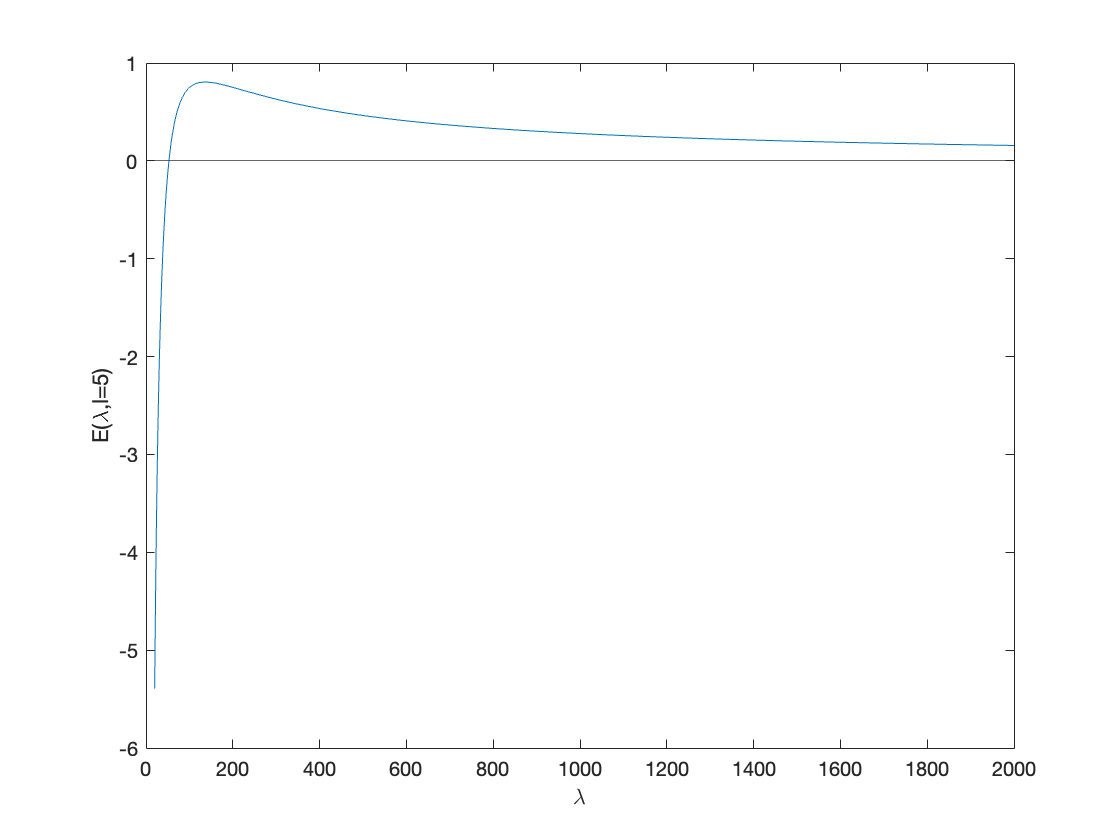
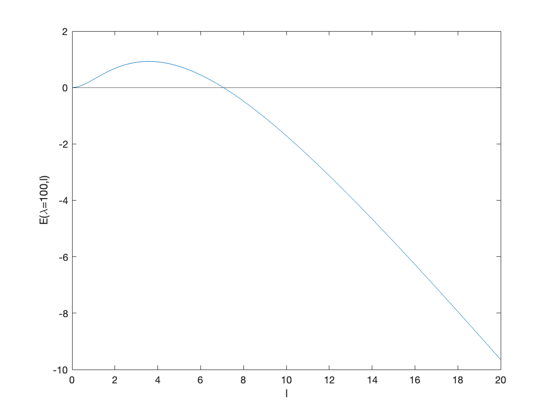
Figure 1. Fix $G_{0}\cdot c_{B}=100$. Left: plot for $E(\lambda,l)$ with $l=5$ and $\lambda\in[0,2000]$. Right: plot for $E(\lambda,l)$ with $\lambda=100$ and $l\in[0,20]$.

Proposition 3.2.

(1) Given any integer $l\geq 2$, there exists unique $\lambda_{0}^{l}>l^{2}$ such that

(3.16) $$E(\lambda_{0}^{l},l)=\frac{G_{0}c_{B}}{\sqrt{\lambda_{0}}}\left(\frac{\sqrt{\lambda_{0}}-l}{\sqrt{\lambda_{0}}+1}+\frac{l-\sqrt{\lambda_{0}+l^{2}}}{\sqrt{\lambda_{0}+l^{2}}+\sqrt{1+l^{2}}}\right)=0.$$

(2) Given any $\lambda>1$, there exists a unique $l_{0}>0$, which may not be an integer, such that $E(\lambda,l_{0})=0$. Furthermore, $E(\lambda,l)\neq 0$ for any $l\neq 0\text{ or }l_{0}$.

In the first part, the fact $\lambda_{0}^{l}>l^{2}$ holds, since one can easily check that $E(\lambda,l)<0$ for any $\lambda\leq l^{2}$. The existence of $\lambda_{0}^{l}$ can be shown by checking the limits

$$\lim_{\lambda\rightarrow 0}E(\lambda,l)=-\infty,\quad\lim_{\lambda\rightarrow+\infty}E(\lambda,l)=0^{+}.$$

And the uniqueness can be checked by directly checking its derivative. In the second part, the existence of $l_{0}$ was proved in [16] by checking the asymptote. Again, the uniqueness can be verified directly.

As we shall show Proposition 3.2 allows us to justify the existence of nonsymmetric traveling waves solutions to (1.1) in the above tube-like domain by applying the Crandall-Rabinowitz Theorem to a functional equation.

4. Bifurcation Analysis

In this section, we justify the existence of non-symmetric traveling wave solutions in (1.1) by relating it to the non-trivial bifurcation branch of a functional equation and conclude by a Crandall–Rabinowitz argument. The framework of utilizing Crandall–Rabinowitz theorem to study the bifurcation behavior of free boundary models was proposed initially by Friedman in [4], then extensively employed to study the bifurcation phenomenon in different tumor growth models, see [18, 4, 37].

We begin with introducing the notations and reviewing the model. Recall that $\Omega$ denotes the tube-like domain defined in (3.15), and $\Omega_{0}$ be the symmetric tumor region in the same manner as (3.5), and we further restrict $l\in\mathbb{N}$. Then, we consider a perturbed tumor region $\Omega_{\epsilon}$ with respect to $\Omega_{0}$,

(4.1) $$\Omega_{\epsilon}=\left\{(x,y)|x\leq\epsilon\xi(y),\quad y\in[-\pi,\pi]\right\},$$

where $0<\epsilon\ll 1$, and $\xi(y)$ is a $2\pi$ periodic even function that characterize the boundary profile. Thus, the boundary can be represented as

(4.2) $$\mathcal{B}_{\epsilon}=\left\{(x,y)|x=\epsilon\xi(y),\quad y\in[-\pi,\pi]\right\}.$$

We employ $(c^{\text{(i)}},c^{\text{(o)}},p^{\text{(i)}})$ to denote the solution to equations (3.1) and (3.3), but with the domain and boundary replaced by $\Omega_{\epsilon}$ and $\mathcal{B}_{\epsilon}$, respectively. More precisely, $(c^{\text{(i)}},c^{\text{(o)}},p^{\text{(i)}})$ solves the following system:

(4.3a) $$-\Delta c^{\text{(i)}}+\lambda c^{\text{(i)}} =0, \qquad\text{in}\quad\Omega_{\epsilon},$$

(4.3b) $$-\Delta c^{\text{(o)}}+c^{\text{(o)}} =c_{B}, \qquad\text{in}\quad\Omega\setminus\Omega_{\epsilon},$$

(4.3c) $$c^{\text{(i)}} =c^{\text{(o)}}, \qquad\text{on}\quad\mathcal{B}_{\epsilon},$$

(4.3d) $$\frac{\partial}{\partial n}c^{\text{(i)}} =\frac{\partial}{\partial n}c^{\text{(o)}}, \qquad\text{on}\quad\mathcal{B}_{\epsilon},$$

(4.3e) $$c_{\epsilon}=c^{\text{(i)}}+c^{\text{(o)}} <\infty, \qquad\text{in}\quad\Omega,$$

(4.3f) $$-\Delta p^{\text{(i)}} =G_{0}c^{\text{(i)}}, \qquad\text{in}\quad\Omega_{\epsilon},$$

(4.3g) $$p^{\text{(i)}} =0, \qquad\text{on}\quad\mathcal{B}_{\epsilon},$$

(4.3h) $$p^{\text{(i)}} <\infty, \qquad\text{in}\quad\Omega_{\epsilon}.$$

Then, we further extend the pressure to the whole $$\Omega p_{\epsilon}$$, denote as , such that

(4.3i) $$p_{\epsilon}=p^{\text{(i)}}+p^{\text{(o)}}$$

with $$p^{\text{(o)}}$$ solves the following PDE:

(4.3j) $$-\Delta p^{\text{(o)}} =G_{0}c^{\text{(o)}}, \qquad\text{in}\quad\Omega\setminus\Omega_{\epsilon},$$

(4.3k) $$p^{\text{(o)}} =0, \qquad\text{on}\quad\mathcal{B}_{\epsilon},$$

(4.3l) $$\frac{\partial}{\partial n}p^{\text{(o)}} =\frac{\partial}{\partial n}p^{\text{(i)}}, \qquad\text{on}\quad\mathcal{B}_{\epsilon}.$$

Note that we introduce $p^{\text{(o)}}$ for technical requirements instead of physical, and we do not require $p^{\text{(o)}}<\infty$ in $\Omega\setminus\Omega_{\epsilon}$. Without the perturbation (when $\epsilon=0$), the solution to (4.3j)-(4.3l) is given by

(4.4) $$p_{0}^{\text{(o)}}(x)=G_{0}c_{B}\left(-\frac{x^{2}}{2}+\frac{\sqrt{\lambda}}{\sqrt{\lambda}+1}e^{-x}+\frac{\lambda-1}{\sqrt{\lambda}(\sqrt{\lambda}+1)}x-\frac{\sqrt{\lambda}}{\sqrt{\lambda}+1}\right),\qquad x\geq 0.$$

To justify the existence of non-symmetric traveling wave solutions in (4.3), we first introduce the following nonlinear functional map:

(4.5) $$F(\xi,\lambda)=-\frac{\partial p_{\epsilon}}{\partial x}\Big{|}_{\mathcal{B}_{\epsilon}}-\sigma_{0}(\lambda),$$

where, as before, the periodic even function $\xi(y)$ stands for the boundary profile, and $\lambda>0$ presents the consumption rate. We emphasize that for the map $F(\xi,\lambda)$ we view $\lambda$ as an index parameter and $\xi$ as the independent variable. Regarding the right-hand side of (4.5), $p_{\epsilon}$ stands for the pressure function associated with the profile $\xi(y)$; and $\sigma_{0}(\lambda)$, given in (3.7), represents the traveling speed of the symmetric solution. Then we look for the solution to the functional equation

(4.6) $$F(\xi,\lambda)=0,$$

since these solutions correspond to the traveling wave solutions to (4.3). In particular, the symmetric solutions correspond to the trivial solution $(0,\lambda)$. We aim to show that for proper consumption rate $\lambda$, it can induce a non-trivial solution branch $(\xi(y),\lambda)$, with $\xi(y)\neq 0$. The existence of such non-trivial bifurcation branches implies that (4.3) admits symmetric breaking traveling wave solutions.

To find the non-trivial bifurcation branch to (4.6), we adopt the framework proposed by Friedman, using the Crandrall-Rabinowitz theorem (see Theorem 4.3). Crandall Rabinowitz theorem is developed to study the bifurcation behavior in nonlinear equations. It provides conditions under which solutions branch off from a trivial solution in nonlinear operator equations. As a useful analysis tool, the Crandall Rabinowitz theorem has been widely applied to study the existence and stability of solutions in nonlinear systems, see, e.g., [4, 27, 28, 43]. In particular, Friedman et al. first employed it to study the symmetric breaking solutions to free boundary problems and tumor growth models [4, 17, 19].

To adopt Friedman’s framework to our case, we carry out the main steps as follows:

1. determine the Fréchet derivative of $F(\xi,\lambda)$ with respect to $\xi\in X$ ($X$ is some function space to be specified later) on the line $(0,\lambda)$, denote it as $F_{\xi}(0,\lambda):=\frac{d}{d\xi}F(0,\lambda)$; and show the Fréchet derivative $F_{\xi}(0,\lambda)$, as a bounded linear operator, can be further characterized in terms of an eigenvalue problem; we then find the complete basis of eigenfunctions with distinct eigenvalues (see equation (4.16)).

2. for each $2\leq l\in\mathbb{N}$, we can determine a bifurcation point $(0,\lambda_{0}^{l})$ to the functional equation $F(\xi,\lambda)=0$ by utilizing the explicit expression of the eigenvalues (see (3.16));

3. conclude $\left\{(0,\lambda_{0}^{l})\right\}_{l=2}^{\infty}$ are indeed bifurcation points to $F(\xi,\lambda)=0$ by verifying the Fréchet derivative at these points, $F_{\xi}(0,\lambda_{0}^{l})$, satisfies the bifurcation conditions in the Crandall-Rabinowitz theorem. More specifically, we verify our choice of $\lambda_{0}^{l}$ ensures that only the $l$-th eigenvalue of $F_{\xi}(0,\lambda_{0}^{l})$ degenerates (equals zero). Also note that for every fixed $\lambda_{0}$, there is a spectural gap between this mode and other modes. So the limit can pass.

To accomplish the first two steps above, we need to first look into the linearized system of (4.3). We investigate it in the following subsection.

4.1. The linearized system

We devote this section to studying the linearization of system (4.3), which is closely related to our previous study in [16].

To begin with, we denote $c_{\epsilon}=c^{\text{(i)}}+c^{\text{(o)}}$, $p_{\epsilon}=p^{\text{(i)}}+p^{\text{(o)}}$, and analogously for

(4.7) $$c_{0}=c_{0}^{\text{(i)}}+c_{0}^{\text{(o)}},\quad c_{1}=c_{1}^{\text{(i)}}+c_{1}^{\text{(o)}},\quad p_{0}=p_{0}^{\text{(i)}}+p_{0}^{\text{(o)}},\quad p_{1}=p_{1}^{\text{(i)}}+p_{1}^{\text{(o)}}.$$

Since the perturbation is small, i.e., $0<\epsilon\ll 1$, the solutions $(c_{\epsilon},p_{\epsilon})$ possess the following asymptotic expansion with respect to $\epsilon$:

(4.8a) $$c_{\epsilon}(x,y) =c_{0}(x)+\epsilon c_{1}(x,y)+O(\epsilon^{2}),$$

(4.8b) $$p_{\epsilon}(x,y) =p_{0}(x)+\epsilon p_{1}(x,y)+O(\epsilon^{2}),$$

with the zero-order terms represent the solutions to the unperturbed problem (the symmetric solution).

Utilizing the expansion (4.8), we can use Taylor expansion to evaluate $c^{\text{(i)}}$ and $\frac{\partial}{\partial x}c^{\text{(i)}}$ on the perturbed boundary in the following way

(4.9a) $$c^{\text{(i)}}|_{\mathcal{B}_{\epsilon}} =c^{\text{(i)}}(\epsilon\xi,y)$$

$$=c_{0}^{\text{(i)}}(\epsilon\xi)+\epsilon c_{1}^{\text{(i)}}(\epsilon\xi,y)+O(\epsilon^{2})$$

$$=c_{0}^{\text{(i)}}(0)+\epsilon\xi\frac{\partial}{\partial x}c_{0}^{\text{(i)}}(0)+\epsilon c_{1}^{\text{(i)}}(0,y)+O(\epsilon^{2}),$$

(4.9b) $$\frac{\partial}{\partial x}c^{\text{(i)}}|_{\mathcal{B}_{\epsilon}} =\frac{\partial}{\partial x}c^{\text{(i)}}(\epsilon\xi,y)$$

$$=\frac{\partial}{\partial x}c_{0}^{\text{(i)}}(\epsilon\xi)+\epsilon\frac{\partial}{\partial x}c_{1}^{\text{(i)}}(\epsilon\xi,y)+O(\epsilon^{2})$$

$$=\frac{\partial}{\partial x}c_{0}^{\text{(i)}}(0)+\epsilon\xi\frac{\partial^{2}}{\partial x^{2}}c_{0}^{\text{(i)}}(0)+\epsilon\frac{\partial}{\partial x}c_{1}^{\text{(i)}}(0,y)+O(\epsilon^{2}).$$

Similarly, for $c^{\text{(o)}}$, $p^{\text{(i)}}$, and $p^{\text{(o)}}$ we have

(4.10a) $$c^{\text{(o)}}|_{\mathcal{B}_{\epsilon}} =c_{0}^{\text{(o)}}(0)+\epsilon\xi\frac{\partial}{\partial x}c_{0}^{\text{(o)}}(0)+\epsilon c_{1}^{\text{(o)}}(0,y)+O(\epsilon^{2}),$$

(4.10b) $$\frac{\partial}{\partial x}c^{\text{(o)}}|_{\mathcal{B}_{\epsilon}} =\frac{\partial}{\partial x}c_{0}^{\text{(o)}}(0)+\epsilon\xi\frac{\partial^{2}}{\partial x^{2}}c_{0}^{\text{(o)}}(0)+\epsilon\frac{\partial}{\partial x}c_{1}^{\text{(o)}}(0,y)+O(\epsilon^{2}),$$

(4.10c) $$p^{\text{(i)}}|_{\mathcal{B}_{\epsilon}} =p^{\text{(i)}}_{0}(0)+\epsilon\xi\frac{\partial}{\partial x}p^{\text{(i)}}_{0}(0)+\epsilon p^{\text{(i)}}_{1}(0,y)+O(\epsilon^{2}),$$

(4.10d) $$\frac{\partial}{\partial x}p^{\text{(i)}}|_{\mathcal{B}_{\epsilon}} =\frac{\partial}{\partial x}p^{\text{(i)}}_{0}(0)+\epsilon\xi\frac{\partial^{2}}{\partial x^{2}}p^{\text{(i)}}_{0}(0)+\epsilon\frac{\partial}{\partial x}p^{\text{(i)}}_{1}(0,y)+O(\epsilon^{2}),$$

(4.10e) $$p^{\text{(o)}}|_{\mathcal{B}_{\epsilon}} =p^{\text{(o)}}_{0}(0)+\epsilon\xi\frac{\partial}{\partial x}p^{\text{(o)}}_{0}(0)+\epsilon p^{\text{(o)}}_{1}(0,y)+O(\epsilon^{2}),$$

(4.10f) $$\frac{\partial}{\partial x}p^{\text{(o)}}|_{\mathcal{B}_{\epsilon}} =\frac{\partial}{\partial x}p^{\text{(o)}}_{0}(0)+\epsilon\xi\frac{\partial^{2}}{\partial x^{2}}p^{\text{(o)}}_{0}(0)+\epsilon\frac{\partial}{\partial x}p^{\text{(o)}}_{1}(0,y)+O(\epsilon^{2}).$$

Plugging the expansion (4.8) into (4.3), the zero-order terms are canceled out, and we collect the terms of order $O(\epsilon)$. Regarding the nutrient, the first order terms solve the following boundary value problem

(4.11a) $$-\Delta c_{1}^{\text{(i)}}+\lambda c_{1}^{\text{(i)}} =0,$$

(4.11b) $$-\Delta c_{1}^{\text{(o)}}+c_{1}^{\text{(o)}} =0,$$

(4.11c) $$c_{1}^{\text{(i)}}(0,y) =c_{1}^{\text{(o)}}(0,y),$$

(4.11d) $$\xi\cdot\frac{\partial^{2}}{\partial x^{2}}c_{0}^{\text{(i)}}(0)+\frac{\partial}{\partial x}c_{1}^{\text{(i)}}(0,y) =\xi\cdot\frac{\partial^{2}}{\partial x^{2}}c_{0}^{\text{(o)}}(0)+\frac{\partial}{\partial x}c_{1}^{\text{(o)}}(0,y),$$

(4.11e) $$c_{1}^{\text{(i)}}(-\infty,y) <\infty,$$

(4.11f) $$c_{1}^{\text{(o)}}(+\infty,y) <\infty.$$

While, for pressure, the first order terms solve

(4.12a) $$-\Delta p^{\text{(i)}}_{1} =G_{0}c_{1}^{\text{(i)}},$$

(4.12b) $$\xi\cdot\frac{\partial}{\partial x}p^{\text{(i)}}_{0}(0)+p^{\text{(i)}}_{1}(0,y) =0,$$

(4.12c) $$p^{\text{(i)}}_{1}(-\infty,y) <\infty,$$

(4.12d) $$-\Delta p^{\text{(o)}}_{1} =G_{0}c_{1}^{\text{(o)}},$$

(4.12e) $$\xi\cdot\frac{\partial}{\partial x}p^{\text{(o)}}_{0}(0)+p^{\text{(o)}}_{1}(0,y) =0,$$

(4.12f) $$\xi\cdot\frac{\partial^{2}}{\partial x^{2}}p_{0}^{\text{(i)}}(0)+\frac{\partial}{\partial x}p_{1}^{\text{(i)}}(0,y) =\xi\cdot\frac{\partial^{2}}{\partial x^{2}}p_{0}^{\text{(o)}}(0)+\frac{\partial}{\partial x}p_{1}^{\text{(o)}}(0,y).$$

On the other hand, the first-order terms capture the main reaction to the perturbation and, therefore, variable-separable,

(4.13a) $$c_{1}^{\text{(i)}}(x,y) =\tilde{c}_{1}^{\text{(i)}}(x)\xi(y),\qquad c_{1}^{\text{(o)}}(x,y) =\tilde{c}_{1}^{\text{(o)}}(x)\xi(y),$$

(4.13b) $$p^{\text{(i)}}_{1}(x,y) =\tilde{p}^{\text{(i)}}_{1}(x)\xi(y),\qquad p^{\text{(o)}}_{1}(x,y) =\tilde{p}^{\text{(o)}}_{1}(x)\xi(y).$$

In particular, when $\xi(y)=\cos{ly}$ the first order terms reduce to the form of (3.10), and the solutions to (4.11) and (4.12) are given by the single mode perturbation problem solved in Section 3.2. Note that through we did not provide the expression of $p^{\text{(o)}}_{1}$ in (3.13), it is solvable via (4.12) once $c_{1}^{\text{(o)}}$, $p_{0}^{\text{(i)}}$, $p_{0}^{\text{(o)}}$, and $p_{1}^{\text{(i)}}$ are determined.

In the following sections, we will show that the above linearization study helps us to characterize the Fréchet derivative, $F_{\xi}(0,\lambda)$, for any $\lambda>0$.

4.2. Derivation and characterization of $F_{\xi}(0,\lambda)$

In this section, we further determine and characterize the Fréchet derivative $F_{\xi}(0,\lambda)$ based on the calculations in the previous subsection. To begin with, we introduce the following Banach spaces

(4.14a) $$X^{m+\alpha} =\left\{f(y)\in C^{m+\alpha}:f(y)\text{ is }2\pi\text{ periodic and even}\right\};$$

(4.14b) $$X_{1}^{m+\alpha} =\text{closure of the linear space spanned by }\{\cos{jy},j=0,1,2,\dots\}\text{ in }X^{m+\alpha}.$$

Note that all modes are included. Thus, any $\xi(y)\in X_{1}^{m+\alpha}$ can be represented as Fourier series. Then, to determine the Fréchet derivative $F_{\xi}(0,\lambda)$, one needs to justify the expansion (4.8) rigorously, which is equivalent to proof of the following two lemmas.

Lemma 4.1.

If $\xi$ belongs to $C^{3+\alpha}(\mathbb{R})$, $c_{\epsilon}$ and $p_{\epsilon}$ be the solution to the system (4.3), then

$$\|c_{\epsilon}-c_{0}\|_{C^{1+\alpha}(\Omega)} \leq C|\epsilon|\|\xi\|_{C^{3+\alpha}(\mathbb{R})},$$

$$\|p_{\epsilon}-p_{0}\|_{C^{3+\alpha}(\Omega)} \leq C|\epsilon|\|\xi\|_{C^{3+\alpha}(\mathbb{R})},$$

where $C$ is a constant independent of $\epsilon$, and $(c_{0},p_{0})$ stands for the unperturbed solutions given in (3.6) and (4.4).

Lemma 4.2.

If $\xi$ belongs to $C^{3+\alpha}(\mathbb{R})$, $c_{\epsilon}$ and $p_{\epsilon}$ be the solution to (4.3), then

$$\|c_{\epsilon}-c_{0}-\epsilon\hat{c}_{1}\|_{C^{1+\alpha}(\Omega)} \leq C|\epsilon|^{2}\|\xi\|_{C^{3+\alpha}(\mathbb{R})},$$

$$\|p_{\epsilon}-p_{0}-\epsilon\hat{p}_{1}\|_{C^{3+\alpha}(\Omega)} \leq C|\epsilon|^{2}\|\xi\|_{C^{3+\alpha}(\mathbb{R})},$$

where $C$ is a constant independent of $\epsilon$, and $(c_{0},p_{0})$ stands for the unperturbed solutions, $(\hat{c}_{1},\hat{p}_{1})$ corresponds to the Hanzawa transformation (see (4.25)) of the first order terms.

The proof of the above lemmas is standard but cumbersome. To avoid the reader’s distraction, we provide a sketch proof in Section 4.4. For now, we directly use them to determine the Fréchet derivative of $F$. The calculations in Section 4.1 yields

$$F(\xi,\lambda) =-\frac{\partial p_{\epsilon}}{\partial x}\Big{|}_{\mathcal{B}_{\epsilon}}-\sigma_{0}(\lambda)$$

$$=-\left(\partial_{x}^{2}p_{0}(0)+\partial_{x}\tilde{p}_{1}(0)\right)\epsilon\xi+O(\epsilon^{2}).$$

Furthermore, Lemma 4.1 and Lemma 4.2 implie $F$ maps from $X^{m+\alpha}\times\mathbb{R}$ to $X^{m+\alpha}$ for any $m\geq 3$. And, according to (3.14), for $\xi(y)=\cos{ly}$ the above identity reduces to

$$F(\cos{ly},\lambda) =-\left(\partial_{x}^{2}p_{0}^{\text{(i)}}(0)+\partial_{x}\tilde{p}_{1,l}^{\text{(i)}}(0)\right)\epsilon\cos{ly}+O(\epsilon^{2})$$

$$=E(\lambda,l)\epsilon\cos{ly}+O(\epsilon^{2}),$$

equivalently,

(4.15) $$\|F(\cos{ly},\lambda)-F(0,\lambda)-E(\lambda,l)\epsilon\cos{ly}\|_{X^{m+\alpha}}\leq C\epsilon^{2}.$$

Thus, given any $\lambda>0$ the Fréchet derivative $F_{\xi}(0,\lambda)$, as a bounded linear operator, is fully characterized by the following eigenvalue problem

(4.16) $$\left[F_{\xi}(0,\lambda)\right]\cos{ly}=E(\lambda,l)\cos{ly},$$

where the eigenvalue $E(\lambda,l)\in\mathbb{R}$. In the following subsection, we show that based on the above eigenvalue problem and the properties of $E(\lambda,l)$ in Proposition 3.2, we can determine bifurcation points and further conclude the existence of non-trivial bifurcation branches to equation (4.6).

4.3. Existence of non-trivial bifurcation branches

In the seminal work [4], Friedman et al. employed the Crandall-Rabinowitz theorem to show the existence of non-radial symmetric solutions to a tumor growth model developed from [22]. Although, as discussed in the introduction section, (4.3) is derived from the incompressible limit of PME and, therefore, essentially different from the models developed from [22], the bifurcation analysis framework established by Friedman remains applicable. We carry out the bifurcation analysis in this subsection. To begin with, for the reader’s convenience, we present the Crandall-Rabinowitz theorem below.

Theorem 4.3.

Let $W,Z$ be real Banach spaces and ${\mathcal{F}}(w,\mu)$ a $C^{p}$ map, $p\geq 3$, of a neighborhood $(0,\mu_{0})$ in $W\times\mathbb{R}$ into $Z$. For any $\omega\in W$ and $\nu\in\mathbb{R}$, ${\mathcal{F}}_{w}(\omega,\nu):=\frac{d}{dw}F(\omega,\nu)\in\mathcal{L}(W,Z)$, where $\nu$ is viewed as a parameter. Suppose

1. ${\mathcal{F}}(0,\mu)=0$ for all $\mu$ in a neighborhood of $\mu_{0}$,

2. The kernel space of the partial derivative ${\mathcal{F}}_{w}:W\rightarrow Z$ at $(0,\mu_{0})$ is of one dimensional spanned by $w_{0}\in W$, i.e., $\text{Ker}\{{\mathcal{F}}_{w}(0,\mu_{0})\}=\text{span}\{w_{0}\}$.

3. The range of ${\mathcal{F}}_{w}(0,\mu_{0})$ has codimension $1$, i.e., $\text{dim}\{Z/Z_{1}\}=1$ with $Z_{1}=\text{Img}\{{\mathcal{F}}_{w}(0,\mu_{0})\}\subseteq Z$.

4. The derivative ${\mathcal{F}}_{w\mu}(w,r)$, $w\in W,r\in\mathbb{R}$, satisfies $\left[{\mathcal{F}}_{w\mu}(0,\mu_{0})\right]w_{0}\notin Z_{1}$.

Then, $(0,\mu_{0})$ is a bifurcation point of the equation ${\mathcal{F}}(w,\mu)=0$ in the following sense: In a neighborhood of $(0,\mu_{0})$, the set of solutions of ${\mathcal{F}}(w,\mu)=0$ consists of two $C^{p-2}$ smooth curves $\mathcal{C}_{1}$ and $\mathcal{C}_{2}$ which intersect only at the point $(0,\mu_{0})$. Moreover, $\mathcal{C}_{1}$ is the curve $(0,\mu)$ and $\mathcal{C}_{2}$ can be parameterized as follows:

$$\mathcal{C}_{2}:(w(\epsilon),\mu(\epsilon)),\epsilon\text{ small},(w(0),\mu(0))=(0,\mu_{0}),w^{\prime}(0)=w_{0}.$$

To apply Theorem 4.3 to the nonlinear map (4.5), the main ingredient is to find a bifurcation point $(0,\lambda_{0})$ such that the partial derivative $F_{\xi}(0,\lambda_{0})$ satisfies the assumptions in Theorem 4.3. According to Friedman’s framework, it is crucial to check this $\lambda_{0}$ leads the eigenvalue to (4.16) vanish in only one direction, i.e., $E(\lambda_{0},l)=0$ holds for only one specific $l\in\mathbb{N}$. We show that this can be done by utilizing Proposition 3.2. And therefore, (4.3) posses non-symmetric traveling wave solutions. We summarize this main result in the following theorem.

Theorem 4.4.

Consider the nonlinear map (4.5), which maps $X_{1}^{3+\alpha}\times\mathbb{R}$ to $X_{1}^{3+\alpha}$. Assume $0<\epsilon\ll 1$. Then for each integer $l\geq 2$, there exists a $\lambda_{0}^{l}>l^{2}$ such that $(0,\lambda_{0}^{l})$ is a bifurcation point to $F(\xi,\lambda)=0$ in the sense of: In a neighborhood of $(0,\lambda_{0}^{l})$, the set of solutions of $F(\xi,\lambda)=0$ consists of two smooth curves $\mathcal{C}_{1}$ and $\mathcal{C}_{2}$ which intersect only at the point $(0,\lambda_{0}^{l})$. Moreover, $\mathcal{C}_{1}$ is the curve $(0,\lambda)$ and $\mathcal{C}_{2}$ can be parameterized as follows:

$$\mathcal{C}_{2}:(\xi(\epsilon),\lambda(\epsilon)),\epsilon\text{ small},\,(\xi(0),\lambda(0))=(0,\lambda_{0}^{l}),\xi^{\prime}(0)=\cos{ly}.$$

Proof.

According to Proposition 3.2, given any integer $l\geq 2$, we can find an unique $\lambda_{0}^{l}>l^{2}$ such that $E(\lambda_{0}^{l},l)=0$. Then we show $(0,\lambda_{0}^{l})$ is indeed a bifurcation point to (4.6) by verifying the map $F(\xi,\lambda)$ indeed satisfies the conditions for applying Theorem 4.3 with the setting $W=X_{1}^{3+\alpha}$, $Z=X_{1}^{2+\alpha}$, $w=\xi$, $w_{0}=\cos{ly}$, and $\mu=\lambda$.

For the differentiability of $F$, it is equivalent to establishing the regularity of the corresponding PDEs. Firstly, note that the structure of the PDEs guarantees that $F$ maps even $2\pi$-periodic functions to even $2\pi$-periodic functions. Then, Lemma 4.1 and Lemma 4.2 imply that $F$ maps $X_{1}^{3+\alpha}\times\mathbb{R}$ into $X_{1}^{3+\alpha}$. Secondly, by using classical elliptic estimates and Sobolev imbedding theory, one can justify $F(\xi,\mu)$ is differentiable to any order by repeating the process in the same manner as Lemma 4.1 and Lemma 4.2. Therefore, $F(\xi,\lambda)$ is $C^{p}$ with $p\geq 3$.

Next, we verify the assumptions (1) to (4) hold for $F(\xi,\lambda)$ at the point $(0,\lambda_{0}^{l})$. Firstly, (1) obviously holds since these trivial solutions correspond to the symmetry solutions. Regarding assumptions (2) and (3), recall that $F_{\xi}(0,\lambda)$ as a bounded linear operator is characterized by the eigenvalue problem (4.16). Thus, to check (2) and (3), it is sufficient for us to check that our choice of $\lambda_{0}^{l}$ ensures:

(4.17) $$E(\lambda_{0}^{l},j)\neq 0\quad\text{for any }\,j\neq l;\quad\text{and}\quad E(\lambda_{0}^{l},l)=0.$$

Based on Proposition 3.2 and the way of chosen $\lambda_{0}^{l}$, condition (4.17) indeed holds. Also note that for every fixed $\lambda_{0}>0$, there is a spectral gap between the $l$-th mode and other modes. So the limit can pass. Finally, for assumption (4), it is sufficient for us to show $\partial_{\lambda}E(\lambda_{0}^{l},l)\neq 0$. Indeed,

$$\partial_{\lambda}E(\lambda_{0}^{l},l) =\frac{1}{2\sqrt{\lambda_{0}^{l}}}\left(\frac{l+1}{\sqrt{\lambda_{0}^{l}}(\sqrt{\lambda_{0}^{l}}+1)^{2}}-\frac{l+\sqrt{1+l^{2}}}{\sqrt{\lambda_{0}^{l}+l^{2}}(\sqrt{\lambda_{0}^{l}+l^{2}}+\sqrt{1+l^{2}})^{2}}\right)$$

$$>\frac{l+1}{2\sqrt{\lambda_{0}^{l}}}\left(\frac{1}{\sqrt{\lambda_{0}^{l}}(\sqrt{\lambda_{0}^{l}}+1)^{2}}-\frac{1}{\sqrt{\lambda_{0}^{l}+l^{2}}(\sqrt{\lambda_{0}^{l}+l^{2}}+\sqrt{1+l^{2}})^{2}}\right)>0,$$

where we used condition (3.16) to derive the first identity. Thus,

(4.18) $$\left[F_{\xi\lambda}(0,\lambda_{0}^{l})\right]\cos{ly}=\left[\partial_{\lambda}E(\lambda_{0}^{l},l)\right]\cos{ly}\notin\text{Img}\left[F_{\xi}(0,\lambda_{0}^{l})\right].$$

By now, we have finished verifying all the assumptions in the Crandall-Rabinowitz theorem. Therefore, $(0,\lambda_{0}^{l})$ is a bifurcation point to (4.6) and generates a non-trivial solution branch. As we interpreted before, this non-trivial solution branch corresponds to the non-symmetric traveling wave solutions to (4.3). ∎

4.4. Justification of the expansion

We devote this section to the proof of Lemma 4.1 and Lemma 4.2. To begin with, recall that $\Omega$ is the tube-like domain defined in (3.15). $\Omega_{0}$ and $\Omega_{\epsilon}$ corresponds to the unperturbed and perturbed tumor region respectively. For concision, we denote the complementary sets as

(4.19) $$\Omega_{0}^{\text{c}}=\Omega\setminus\Omega_{0},\qquad\Omega_{\epsilon}^{\text{c}}=\Omega\setminus\Omega_{\epsilon}.$$

Now, we provide the proof of Lemma 4.1 as follows.

Proof.

Note that if we denote $c^{\delta}=c_{\epsilon}-c_{0}$, then it satisfies

(4.20a) $$-\Delta c^{\delta}+\lambda c^{\delta} =0, \qquad\text{in}\quad\Omega_{\epsilon}\cap\Omega_{0}:=\Omega_{1};$$

(4.20b) $$-\Delta c^{\delta}+\lambda c^{\delta} =(1-\lambda)c_{0}-c_{B}, \qquad\text{in}\quad\Omega_{\epsilon}\cap\Omega_{0}^{\text{c}}:=\Omega_{2};$$

(4.20c) $$-\Delta c^{\delta}+c^{\delta} =(\lambda-1)c_{0}+c_{B}, \qquad\text{in}\quad\Omega_{\epsilon}^{\text{c}}\cap\Omega_{0}:=\Omega_{3};$$

(4.20d) $$-\Delta c^{\delta}+c^{\delta} =0, \qquad\text{in}\quad\Omega_{\epsilon}^{\text{c}}\cap\Omega_{0}^{\text{c}}:=\Omega_{4}.$$

Write them in a single equation, one gets

(4.21) $$-\Delta c^{\delta}+\left(\lambda\cdot\chi_{\Omega_{\epsilon}}+\chi_{\Omega_{\epsilon}^{\text{c}}}\right)c^{\delta}=\left((1-\lambda)c_{0}-c_{B}\right)\cdot\left(\chi_{\Omega_{2}}-\chi_{\Omega_{3}}\right),\qquad\text{in}\quad\Omega.$$

Observe the facts that $\lambda\chi_{\Omega_{\epsilon}}+\chi_{\Omega_{\epsilon}}^{\text{c}}$ can be treated as a function in $L^{\infty}(\Omega)$, $c_{0}$ has already been solved explicitly on $\Omega$. Furthermore, the areas $|\Omega_{2}|$ and $|\Omega_{3}|$ are both bounded by $\epsilon\|\xi\|_{C^{3+\alpha}(\mathbb{R})}$. Then, the classical $W^{2,p}$ estimate of elliptic equations and Sobolev embedding theory together yield the first inequality in Lemma 4.1. More precisely, for any $p>2$ and $\alpha=1-2/p$ one has

$$\|c^{\delta}\|_{C^{1+\alpha}(\Omega)}\leq\|c^{\delta}\|_{W^{2,p}(\Omega)}\leq\|\left((1-\lambda)c_{0}-c_{B}\right)\cdot\left(\chi_{\Omega_{2}}-\chi_{\Omega_{3}}\right)\|_{L^{p}(\Omega)}\leq C|\epsilon|\|\xi\|_{C^{3+\alpha}(\mathbb{R})}.$$

Finally, send $p\rightarrow\infty$ to complete the proof.

For the second inequality in Lemma 4.1, one can easily write down the equation and boundary condition for $p^{\delta}=p_{\epsilon}-p_{0}$ on $\bar{\Omega}_{\epsilon}$, that is

(4.22a) $$-\Delta p^{\delta} =G_{0}c^{\delta}, \qquad\text{in}\quad\Omega_{\epsilon},$$

(4.22b) $$p^{\delta} =-p_{0}, \qquad\text{on}\quad\mathcal{B}_{\epsilon}.$$

Note that $p_{0}=p_{0}^{\text{(i)}}+p_{0}^{\text{(o)}}$ has already been solved on $\Omega$, in particular for $p_{0}|_{\mathcal{B}_{\epsilon}}$. Thus, by using Schauder estimate one has

(4.23) $$\|p^{\delta}\|_{C^{3+\alpha}(\bar{\Omega}_{\epsilon})}\leq G_{0}\|c^{\delta}\|_{C^{1+\alpha}(\Omega_{\epsilon})}+\|p_{0}\|_{C^{3+\alpha}(\mathcal{B}_{\epsilon})}\leq C|\epsilon|\|\xi\|_{C^{3+\alpha}(\mathbb{R})}.$$

∎

Next, observe the fact that $(c^{\text{(i)}},c^{\text{(o)}},p^{\text{(i)}},p^{\text{(o)}})$ are defined on $\Omega_{\epsilon}$ or $\Omega_{\epsilon}^{c}$ respectively. However, the first-order terms $(c_{1}^{\text{(i)}},c_{1}^{\text{(o)}},p_{1}^{\text{(i)}},p_{1}^{\text{(o)}})$ are only defined on $\Omega_{0}$ or $\Omega_{0}^{c}$. Therefore, we need to transform them to $\Omega_{\epsilon}$ or $\Omega_{\epsilon}^{c}$ by Hanzawa transformation ${\mathcal{H}}_{\epsilon}$, which is defined as follows:

(4.24) $$(x,y)={\mathcal{H}}_{\epsilon}(x^{\prime},y^{\prime})=(x^{\prime}+{\mathcal{I}}(x^{\prime})\epsilon\xi,y^{\prime}),$$

where ${\mathcal{I}}$ is defined by:

$${\mathcal{I}}\in C^{\infty},\quad{\mathcal{I}}(\zeta)=\left\{\begin{array}[]{cc}&0,\quad\text{if}\quad|\zeta|\geq\frac{3}{4}\delta,\\ &1,\quad\text{if}\quad|\zeta|<\frac{3}{4}\delta,\end{array}\right.,\quad\text{with}\quad\left|\frac{d^{k}{\mathcal{I}}}{d\zeta^{k}}\right|<\frac{C}{\delta^{k}},$$

where $\delta$ is a small positive scalar. Thus, ${\mathcal{H}}_{\epsilon}$ maps $\Omega_{0}$ onto $\Omega_{\epsilon}$, and maps $\Omega_{0}^{c}$ onto $\Omega_{\epsilon}^{c}$. We further denote

(4.25a) $$\hat{c}_{1}^{\text{(i)}}(x,y) =c_{1}^{\text{(i)}}({\mathcal{H}}_{\epsilon}^{-1}(x,y)),\qquad\hat{c}_{1}^{\text{(o)}}(x,y) =c_{1}^{\text{(o)}}({\mathcal{H}}_{\epsilon}^{-1}(x,y)),$$

(4.25b) $$\hat{p}_{1}^{\text{(i)}}(x,y) =p_{1}^{\text{(i)}}({\mathcal{H}}_{\epsilon}^{-1}(x,y)),\qquad\hat{p}_{1}^{\text{(o)}}(x,y) =p_{1}^{\text{(o)}}({\mathcal{H}}_{\epsilon}^{-1}(x,y)).$$

Now, we turn to the proof of Lemma 4.2. The detail of the proof is cumbersome, but the idea is quite simple and in the same manner as the proof of Lemma 3.1. Therefore, we only provide a sketch of it.

Proof.

The proof is similar to that of Lemma 4.1. Denote $c^{\delta}:=c_{\epsilon}-c_{0}-\epsilon\hat{c}_{1}$ and similarly for $p^{\delta}:=p_{\epsilon}-p_{0}-\epsilon\hat{p}_{1}$. Then, one is able to write out the equation for $c^{\delta}$ on the whole $\Omega$. Then, employ $W^{2,p}$ estimate of the elliptic equations and the embedding theory to obtain the estimate for the nutrient first, as we did in Lemma 4.1. However, to do this, one needs to compute the first and second derivatives of $\hat{c}_{1}$ with respect to $(x,y)$, which further requires us to consider the change of variables induced by the Hanzawa transformation. This process is cumbersome but standard. Therefore, we refer the reader to Theorem 4.5 in [37] for a similar proof. Once the estimate of the nutrient is obtained, one can further obtain the pressure estimate by Schauder estimate in the same manner as Lemma 4.1. ∎

References

- [1] John A Adam and Nicola Bellomo. A survey of models for tumor-immune system dynamics. Springer Science & Business Media, 1997.
- [2] M Ben Amar, C Chatelain, and Pasquale Ciarletta. Contour instabilities in early tumor growth models. Physical review letters, 106(14):148101, 2011.
- [3] Samiha Belmor. Existence result and free boundary limit of a tumor growth model with necrotic core. arXiv:2210.07014, 2022.
- [4] Andrei Borisovich and Avner Friedman. Symmetry-breaking bifurcations for free boundary problems. Indiana University mathematics journal, pages 927–947, 2005.
- [5] H M_ Byrne and MAJ Chaplain. Growth of necrotic tumors in the presence and absence of inhibitors. Mathematical biosciences, 135(2):187–216, 1996.
- [6] Xinfu Chen and Avner Friedman. A free boundary problem for an elliptic-hyperbolic system: an application to tumor growth. SIAM Journal on Mathematical Analysis, 35(4):974–986, 2003.
- [7] Katy Craig, Inwon Kim, and Yao Yao. Congested aggregation via Newtonian interaction. Arch. Ration. Mech. Anal., 227(1):1–67, 2018.
- [8] Vittorio Cristini, Hermann B Frieboes, Robert Gatenby, Sergio Caserta, Mauro Ferrari, and John Sinek. Morphologic instability and cancer invasion. Clinical Cancer Research, 11(19):6772–6779, 2005.
- [9] Shangbin Cui. Formation of necrotic cores in the growth of tumors: analytic results. Acta Mathematica Scientia, 26(4):781–796, 2006.
- [10] Shangbin Cui and Avner Friedman. Analysis of a mathematical model of the growth of necrotic tumors. Journal of Mathematical Analysis and Applications, 255(2):636–677, 2001.
- [11] Noemi David and Benoît Perthame. Free boundary limit of a tumor growth model with nutrient. J. Math. Pures Appl. (9), 155:62–82, 2021.
- [12] Tomasz Debiec, Benoît Perthame, Markus Schmidtchen, and Nicolas Vauchelet. Incompressible limit for a two-species model with coupling through Brinkman’s law in any dimension. J. Math. Pures Appl. (9), 145:204–239, 2021.
- [13] Tomasz Debiec and Markus Schmidtchen. Incompressible limit for a two-species tumour model with coupling through Brinkman’s law in one dimension. Acta Appl. Math., 169:593–611, 2020.
- [14] Xu’an Dou, Chengfeng Shen, and Zhennan Zhou. Tumor growth with a necrotic core as an obstacle problem in pressure. arXiv preprint arXiv:2309.00065, 2023.
- [15] Yu Feng, Liu Liu, and Zhennan Zhou. A unified bayesian inversion approach for a class of tumor growth models with different pressure laws. ESAIM: Mathematical Modelling and Numerical Analysis, 58(2):613–638, 2024.
- [16] Yu Feng, Min Tang, Xiaoqian Xu, and Zhennan Zhou. Tumor boundary instability induced by nutrient consumption and supply. Zeitschrift für angewandte Mathematik und Physik, 74(3):107, 2023.
- [17] Avner Friedman and Bei Hu. Bifurcation from stability to instability for a free boundary problem arising in a tumor model. Archive for rational mechanics and analysis, 180:293–330, 2006.
- [18] Avner Friedman and Bei Hu. Bifurcation for a free boundary problem modeling tumor growth by stokes equation. SIAM Journal on Mathematical Analysis, 39(1):174–194, 2007.
- [19] Avner Friedman and Bei Hu. Stability and instability of liapunov-schmidt and hopf bifurcation for a free boundary problem arising in a tumor model. Transactions of the American Mathematical Society, 360(10):5291–5342, 2008.
- [20] Avner Friedman and Fernando Reitich. Analysis of a mathematical model for the growth of tumors. Journal of mathematical biology, 38:262–284, 1999.
- [21] HP Greenspan. Models for the growth of a solid tumor by diffusion. Studies in Applied Mathematics, 51(4):317–340, 1972.
- [22] HP Greenspan. On the growth and stability of cell cultures and solid tumors. Journal of theoretical biology, 56(1):229–242, 1976.
- [23] Nestor Guillen, Inwon Kim, and Antoine Mellet. A Hele-Shaw limit without monotonicity. Arch. Ration. Mech. Anal., 243(2):829–868, 2022.
- [24] Wenrui Hao, Jonathan D Hauenstein, Bei Hu, Yuan Liu, Andrew J Sommese, and Yong-Tao Zhang. Bifurcation for a free boundary problem modeling the growth of a tumor with a necrotic core. Nonlinear Analysis: Real World Applications, 13(2):694–709, 2012.
- [25] Qingyou He, Hai-Liang Li, and Benoît Perthame. Incompressible limit of porous media equation with chemotaxis and growth. arXiv preprint arXiv:2312.16869, 2023.
- [26] Qingyou He, Hai-Liang Li, and Benoît Perthame. Incompressible limits of the patlak-keller-segel model and its stationary state. Acta Applicandae Mathematicae, 188(1):11, 2023.
- [27] Joan Mateu Hmidi, Taoufik and Joan Verdera. Boundary regularity of rotating vortex patches. Archive for rational mechanics and analysis, 209:171–208, 2013.
- [28] J.M. Morel J. I. Diaz and L. Oswald. An elliptic equation with singular nonlinearity. Communications in Partial Differential Equations, 12:1333–1344, 1987.
- [29] Matt Jacobs, Inwon Kim, and Jiajun Tong. Tumor growth with nutrients: Regularity and stability. Communications of the American Mathematical Society, 3(04):166–208, 2023.
- [30] Inwon Kim and Jona Lelmi. Tumor growth with nutrients: stability of the tumor patches. SIAM Journal on Mathematical Analysis, 55(5):5862–5892, 2023.
- [31] Inwon Kim and Antoine Mellet. Incompressible limit of porous medium equation with bistable and monostable reaction terms. arXiv:2208.09450, 2022.
- [32] Inwon Kim, Norbert Požár, and Brent Woodhouse. Singular limit of the porous medium equation with a drift. Advances in Mathematics, 349:682–732, 2019.
- [33] Inwon Kim and Olga Turanova. Uniform convergence for the incompressible limit of a tumor growth model. Ann. Inst. H. Poincaré C Anal. Non Linéaire, 35(5):1321–1354, 2018.
- [34] Jian-Guo Liu, Min Tang, Li Wang, and Zhennan Zhou. An accurate front capturing scheme for tumor growth models with a free boundary limit. Journal of Computational Physics, 364:73–94, 2018.
- [35] Jian-Guo Liu, Min Tang, Li Wang, and Zhennan Zhou. Analysis and computation of some tumor growth models with nutrient: From cell density models to free boundary dynamics. Discrete and Continuous Dynamical Systems - B, 24(7):3011–3035, 2019.
- [36] Jian-Guo Liu and Xiangsheng Xu. Existence and incompressible limit of a tissue growth model with autophagy. SIAM J. Math. Anal., 53(5):5215–5242, 2021.
- [37] Min-Jhe Lu, Wenrui Hao, Bei Hu, and Shuwang Li. Bifurcation analysis of a free boundary model of vascular tumor growth with a necrotic core and chemotaxis. Journal of Mathematical Biology, 86(1):19, 2023.
- [38] Benoît Perthame, Fernando Quirós, Min Tang, and Nicolas Vauchelet. Derivation of a Hele-Shaw type system from a cell model with active motion. Interfaces Free Bound., 16(4):489–508, 2014.
- [39] Benoît Perthame, Fernando Quirós, and Juan Luis Vázquez. The Hele-Shaw asymptotics for mechanical models of tumor growth. Arch. Ration. Mech. Anal., 212(1):93–127, 2014.
- [40] Benoît Perthame, Min Tang, and Nicolas Vauchelet. Traveling wave solution of the hele–shaw model of tumor growth with nutrient. Mathematical Models and Methods in Applied Sciences, 24(13):2601–2626, 2014.
- [41] Benoît Perthame and Nicolas Vauchelet. Incompressible limit of a mechanical model of tumour growth with viscosity. Philos. Trans. Roy. Soc. A, 373(2050):20140283, 16, 2015.
- [42] Jiajun Tong and Yuming Paul Zhang. Convergence of free boundaries in the incompressible limit of tumor growth models, 2024.
- [43] Juncheng Wei. Exact multiplicity for some nonlinear elliptic equations in balls. Proceedings of the American Mathematical Society, 125:3235–3242, 1997.
- [44] Junde Wu. Analysis of a nonlinear necrotic tumor model with two free boundaries. Journal of Dynamics and Differential Equations, 33(1):511–524, 2021.
- [45] Yiyang Ye, Jie Lin, et al. Fingering instability accelerates population growth of a proliferating cell collective. Physical Review Letters, 132(1):018402, 2024.