Bridging Speed and Accuracy to Approximate $K$-Nearest Neighbor Search

Abstract.

Approximate $K$-Nearest Neighbor (AKNN) search in high-dimensional spaces is a critical yet challenging problem. The efficiency of AKNN search largely depends on the computation of distances, a process that significantly affects the runtime. To improve computational efficiency, existing work often opts for estimating approximate distances rather than computing exact distances, at the cost of reduced AKNN search accuracy. The recent method of ADSampling has attempted to mitigate this problem by using random projection for distance approximations and adjusting these approximations based on error bounds to improve accuracy. However, ADSampling faces limitations in effectiveness and generality, mainly due to the suboptimality of its distance approximations and its heavy reliance on random projection matrices to obtain error bounds. In this study, we propose a new method that uses an optimal orthogonal projection instead of random projection, thereby providing improved distance approximations. Moreover, our method uses error quantiles instead of error bounds for approximation adjustment, and the derivation of error quantiles can be made independent of the projection matrix, thus extending the generality of our approach. Extensive experiments confirm the superior efficiency and effectiveness of the proposed method. In particular, compared to the state-of-the-art method of ADSampling, our method achieves a speedup of 1.6 to 2.1 times on real datasets with almost no loss of accuracy.

PVLDB Reference Format:
Mingyu Yang et al. PVLDB, 14(1): XXX-XXX, 2020.
doi:XX.XX/XXX.XX

PVLDB Artifact Availability:
The source code, data, and/or other artifacts have been made available at %leave␣empty␣if␣no␣availability␣url␣should␣be␣sethttps://github.com/mingyu-hkustgz/Res-Infer.

1. Introduction

The problem of $K$-Nearest Neighbor (KNN) search in high-dimensional spaces aims to identify the top-$K$ data points in a database $S$ that are closest to a query point $q$. KNN search is of great importance in information retrieval (Liu et al., 2007), data mining (Cover and Hart, 1967), recommendation systems (Schafer et al., [n.d.]), and large language models (Lewis et al., 2020). While effective solutions (such as R-trees) for KNN search exist in low-dimensional spaces, the curse of dimensionality (Indyk and Motwani, 1998) makes exact KNN search prohibitively time-consuming in high-dimensional spaces. As a result, researchers have resorted to a relaxed version of the problem, called Approximate $K$-Nearest Neighbor (AKNN) search, which trades accuracy for efficiency.

Given the importance of AKNN, a variety of AKNN algorithms have been proposed. These algorithms mainly include inverted file-based (Jégou et al., 2011; Babenko and Lempitsky, 2015), graph-based (Malkov et al., 2014; Malkov and Yashunin, 2020; Fu et al., 2022, 2019; Li et al., 2020; Peng et al., 2023), tree-based (Dasgupta and Freund, 2008; Beygelzimer et al., 2006; Ram and Sinha, 2019), and hash-based (Sun et al., 2014; Zheng et al., 2020; Gan et al., 2012; Goemans and Williamson, 1995; Huang et al., 2015, 2017) methods. Conceptually, to search for the AKNN of a query point $q$ in a database $S$, AKNN algorithms can be abstracted into a candidate generation-verification framework: (1) Candidate generation: This involves selecting a subset of points from $S$ as a superset of the returned AKNN. (2) Verification: This involves identifying the top-$K$ points closest to $q$ among the candidates to be returned as the AKNN.

Interestingly, the distinction between different AKNN algorithms lies mostly in the candidate generation phase. For example, inverted file-based methods (such as IVF) use clustering, while graph-based methods (such as HNSW (Malkov and Yashunin, 2020)) use greedy traversal to obtain candidates. Yet, the verification phase of the AKNN algorithms is largely similar across the board. This phase maintains a result queue $Q$ (which can be implemented as a max-heap) to preserve the data points closest to the query point $q$, thereby yielding the final result. Specifically, for a given candidate point $p$, if the distance from this point to the query point $q$ is less than the maximum distance $\tau$ recorded in $Q$, the result queue is updated; otherwise, the vertex is ignored. Thus, distance computation is critical and demanding during the verification phase. In fact, distance computation is the most time-consuming part of AKNN algorithms. For example, for graph-based methods such as HNSW (Malkov and Yashunin, 2020), distance computation accounts for $80\%$ of the total time of AKNN search; for inverted file-based methods such as IVF, distance computation accounts for $90\%$ of the total time cost (Gao and Long, 2023). Thus, speeding up the distance computation becomes the key to speeding up the AKNN search.

Approximate Distance Computation. To compute the (exact) distance between two points in a $D$-dimensional space, one could scan each dimension sequentially, resulting in a time complexity of $O(D)$. To speed up the distance computation and thus increase the efficiency of the AKNN search, an intuitive idea is to compute approximate distances instead of exact distances. Among these, projection and product quantization (Jégou et al., 2011) are two typical approaches to computing approximate distances, each with its own suitable application scenarios. Specifically, projection methods (e.g., PCA) transform the original $D$-dimensional space into a new $d$-dimensional space (where $d<D$), thus reducing the time complexity of distance computation to $O(d)$; Product quantization methods, on the other hand, divide the original space into $M$ subspaces, each of which has a dimension $d$ smaller than the original dimension $D$. By merging the results of the subspaces via a distance look-up table, the time cost of $O(M)$ is achieved.

Figure 1. A comparison of search efficiency (Qps) and accuracy (Top 1-Recall) on the SIFT1M dataset. HNSW uses exact distance calculation, while HNSW${}_{\text{PQ}}$ uses Product Quantization (PQ) and HNSW${}_{\text{PCA}}$ uses PCA (with $d=32$) for approximate distance calculation.

These two approximate distance computation methods can be combined with any AKNN algorithm. However, using approximate distances instead of exact distances greatly reduces the accuracy of the search result. The reason is that during the verification phase, incorrect approximate distances are likely to eject the true KNN points out of the result queue $Q$, causing the final returned data points (i.e., AKNN) to differ significantly from the actual results (i.e., KNN). For example, on the SIFT dataset with one million data points, using projection methods (e.g., PCA) and product quantization methods to compute approximate distances results in a huge decrease in the recall of the top-1 result, as shown in Fig. 1.

Existing Solution. To address the shortcomings of existing distance computation methods in AKNN search, ADSampling (Gao and Long, 2023) was introduced. ADSampling first computes an approximation distance between two points by random projection and obtains an error bound from the projection matrix. The advantage of ADSampling lies in its ability to use error bounds to analyze whether the use of current approximate distances in the verification phase of the AKNN search is sufficient. If not, more accurate distances are computed incrementally until finally an exact distance is calculated. ADSampling has achieved a good balance between speed and accuracy in AKNN search through adjustment by error bounds, and experimental results have confirmed its effectiveness. However, there is still significant room for improvement in its effectiveness and generality.

Effectiveness. ADSampling uses a projection method to obtain approximate distances. Specifically, ADSampling uses a random projection matrix to compute these approximate distances. Yet, within projection methods, a random projection matrix cannot guarantee the minimization of the error between approximate and exact distances. Note that if the approximate distance is sufficiently accurate, then ADSampling does not need to incrementally perform the more time-consuming precise distance calculations. Thus, it is necessary to compute a more accurate approximate distance.

Generality. The error bound plays a critical role in ADSampling because it can determine when the calculation of approximate distances needs to be replaced by exact distance calculations to ensure accuracy. Unfortunately, obtaining the error bound for ADSampling is highly dependent on the random process of generating the projection matrix. This makes ADSampling highly dependent on the random projection matrix, which makes it inapplicable to approximate distances obtained by methods other than random projection.

Our Idea. To address the shortcomings in the effectiveness of ADsampling, we propose new distance computation methods in this paper. Specifically, we decompose the approximate (projected) distance to elucidate the relationship between the projection matrix and the error term (i.e., the gap between the exact distance and the approximate distance). By minimizing the error term, we find that using the optimal orthogonal projection rather than the random projection (as used by ADsampling) results in a theoretically optimal approximate distance. Therefore, we choose to use the orthogonal projection to obtain approximate distances to improve effectiveness.

Furthermore, inspired by the error bounds of ADsampling, we use error quantiles to adjust the approximate distance during the AKNN search. Compared to error bounds, error quantiles contain more information and thus achieve a better balance between speed and efficiency. Also, we decouple the acquisition of error quantiles from the projection matrix and propose a numerical method to compute error quantiles directly. Thanks to the decoupling, our method can now be adapted to arbitrary approximated distances (such as those obtained from product quantization), thereby endowing our proposed approach with the generality that ADsampling lacks. We also discuss how to incorporate the proposed approximate distances and error quantiles into the AKNN search’s verification phase in order to implement a specific AKNN algorithm.

Contributions. We summarize our contributions as follows:

Problem Analysis of the State-of-the-art. We investigated the limitations of the cutting-edge AKNN method, ADSampling. In particular, the use of random projection for ADSampling to compute approximate distances reduces its effectiveness. Furthermore, the error bound used in ADSampling is highly dependent on the random projection matrix used, rendering it difficult to adapt to other approximate distance computation methods and thus losing generality.

A New Projection-Based Distance Computation Method. To obtain the approximate distance, we found that using an optimal orthogonal projection rather than random projections (as in ADSampling) produces the smallest approximation error. In addition, inspired by the use of error bounds in ADSampling, we use a more informative error quantile to indicate when to compute exact distances to ensure accuracy. The adoption of a novel approach for obtaining approximate distance plus the utilization of error quantiles constitutes our new projection-based distance computation method. This method can be integrated with any AKNN algorithm.

A New General Distance Computation Method. We propose a general method for computing distances. Unlike ADSampling, which is only applicable to approximate distances obtained via random projection, our method does not impose any restrictions on how approximate distances are obtained to ensure generality. Specifically, we propose to derive error quantiles from data distributions and use a learning-based approach during the validation phase to decide whether it is necessary to compute precise distances to maintain accuracy in the AKNN search. In addition, we discuss how our general distance computation method can be integrated with existing AKNN algorithms to improve their efficiency.

Extensive Experimental Analysis. We have conducted extensive experiments on a large number of real datasets to validate our methods. The experimental results show that our methods can achieve an acceleration of 1.6 to 2.1 times compared to the state-of-the-art ADSampling. Moreover, our methods show stable performance under different parameter settings, which further illustrates the effectiveness of our methods.

Due to space limitations, some proofs have been omitted and can be found in the technical report (Yang et al., 2024).

2. Preliminaries

Section 2.1 introduces AKNN search problem and algorithms. Then, Section 2.2 discusses the issue of distance computation, an essential component of AKNN search.

Table 1. A Summary of Notations

Notation	Description
$S$	A set of points
$D$	The dimensionality of $S$
$\RR$	The projection(rotate) matrix
$\mathbb{R}^{d}$	$d$-dimensional Euclidean space
$dis,dis^{\prime}$	precise and approximate distance
$N^{ef}$	${\mathsf{HNSW}}$ search parameter
$N^{prob}$	${\mathsf{IVF}}$ search parameter
$\|u,v\|$	The Euclidean distance between $u$ and $v$
$\tau$	The distance threshold
$L$	The linear classifier

2.1. The AKNN Search

Given a dataset $S$ containing $n$ points/vectors in $D$-dimensional space, that is, $S=\{p_{1},p_{2},...,p_{n}\}$, where $p_{i}\in\mathbb{R}^{D}$. We use the squared Euclidean distance to compute the distance $dis(p,q)$ between two points $p$ and $q$, where $dis(p,q)=\|p-q\|^{2}$. The time complexity of computing $dis(p,q)$ is $O(D)$ by scaning each dimension sequentially. The problem of the $K$-Nearest Neighbor (KNN) search is to find the data points in $S$ that are among the top-$K$ smallest distances to a query point $q\in\mathbb{R}^{D}$. Note that there are other widely adopted distance metrics, such as cosine similarity and inner product, that can be transformed into Euclidean distance through simple transformations (Gao and Long, 2023). Table 1 summarizes the commonly used notation.

AKNN Algorithms. Due to the complexity of KNN search, the problem of its relaxed version —Approximate $K$-Nearest Neighbors (AKNN) search — has been proposed. Given a query point $q$, the AKNN search does not require the returned points to be the exact $K$ closest points to $q$, thus sacrificing accuracy for computational efficiency. Currently, AKNN algorithms can be divided mainly into four categories: tree-based (Dasgupta and Freund, 2008), hash-based (Sun et al., 2014; Zheng et al., 2020; Goemans and Williamson, 1995; Gan et al., 2012; Huang et al., 2015, 2017), Inverted File-based(Babenko and Lempitsky, 2015; Jégou et al., 2011), and graph-based (Malkov and Yashunin, 2020; Fu et al., 2022, 2019; Lu et al., 2021; Peng et al., 2023; Harwood and Drummond, 2016; Li et al., 2020).

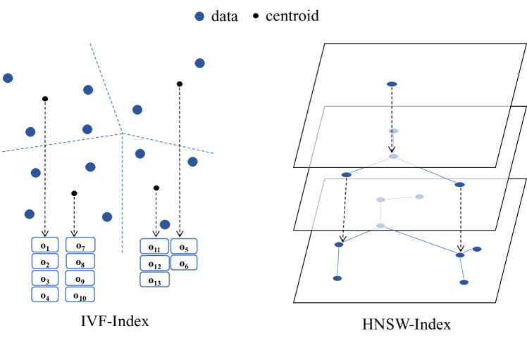
Figure 2. Example of IVF and HNSW

Inverted File-based Algorithms. The basic idea behind Inverted File-based algorithms (see Fig. 2) is to use clustering to divide the points in a dataset $S$ into multiple clusters. This is then used to speed up the AKNN search. Specifically, during the indexing process, IVF uses the $k$-means algorithm to cluster the data points in $S$, constructs a bucket for each cluster, and assigns the data points contained in that cluster to the corresponding bucket. During the query process, for a given query point $q$, IVF first selects the nearest $N^{Probe}$ clusters based on the distance from $q$ to the cluster centroids, retrieves all data points in the corresponding buckets of these nearest clusters as candidates, and then identifies the $K$ nearest neighbors among these candidates. Here, $N^{Probe}$ is a user parameter that controls the trade-off between time and accuracy: as $N^{Probe}$ increases, more clusters are considered, thus improving accuracy at the cost of increased computation time.

Graph-based Algorithms. Graph-based algorithms for approximate nearest neighbor (ANN) search rely on the construction of a navigable graph structure where nodes represent data points and edges connect nodes that are considered nearest neighbors. Hierarchical Navigable Small World (HNSW), a state-of-the-art graph-based algorithm (see Fig. 2), has been recognized for its superior performance in terms of search speed and accuracy. To index HNSW, data points are inserted into a multi-layered graph structure with each layer representing the data in increasingly fine-grained detail. During insertion, each point is connected to a fixed number of closest neighbors, ensuring that each layer retains a navigable small-world network property. In the query process, the search begins by navigating down from the top layer, leveraging the hierarchical small-world structure to efficiently converge on the region closest to the query point. Once reaching the base layer, the algorithm navigates precisely through the neighborhood graph to identify the approximate nearest neighbors to the query point.

Other AKNN Algorithms. Other AKNN algorithms include tree-based and hash-based methods, among others. Tree-based methods identify candidate points through tree routing, while hash-based methods generate candidate points through hash codes, then further identify the result points as AKNN. It is important to note that in practice, these methods are not more appealing than the Inverted File- and graph-based methods due to performance.

2.2. Existing Distance Computation Methods

From the introduction of AKNN algorithms, it is clear that although these algorithms use different approaches to obtain AKNN, they all follow the same candidate generation-verification framework in the query process: In the candidate generation phase, the AKNN algorithms collect a superset of points in $S$ as candidates. In the verification phase, they identify the top-$K$ closest points to a query point $q$ from the candidates as the result to be returned. Note that the methods for generating candidate points differ significantly and thus form different categories of AKNN algorithms, e.g., IVF uses clustering, while HNSW uses traversal to find candidates. However, the verification phase of generating result points from the candidates is actually the same for different AKNN algorithms.

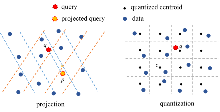
Figure 3. Example of random projection and quantization

The Verification Phase. To find the $K$ result points from the candidates, current AKNN Algorithms often maintain a set of points using a queue $Q$ (usually organized as a max-heap). They examine each candidate point sequentially; for each candidate point $p$, they check whether its distance to the query vertex $q$ is not greater than the maximum threshold $\tau$ recorded in $Q$. If so, the new candidate $p$ is inserted into $Q$ and $Q$ is updated; otherwise, $p$ is ignored.

Approximate Distance Computation. The time to compute distances dominates the runtime of the AKNN search, accounting for 80% of the time complexity in IVF and 90% in HNSW. To improve efficiency, an intuitive idea is to use approximate distances instead of exact distances for the verification phase of the AKNN search. Existing work has proposed two methods for computing approximate distances: projection and product quantization (see Fig. 3). Recall that computing distances by successively scanning dimensions leads to a linear time cost in the dimensionality $D$ of the dataset $S$, these two methods use different approaches to reduce the dimensionality of the data to improve efficiency, and each method has its own appropriate application scenarios.

Projection. Projection methods (such as PCA) map high-dimensional data to a lower-dimensional space, mitigating the curse of dimensionality and facilitating efficient data processing and storage. Specifically, we generally achieve dimensionality reduction by multiplying the vectors in the original space by an orthogonal projection matrix. The advantage of projection methods is that they are relatively easy to implement, involving the construction of projection matrices for matrix multiplication, and allow for the processing of large, high-dimensional data sets in a comparatively short amount of time.

Product Quantization. Product quantization methods (such as OPQ (Jégou et al., 2011)) are widely used for dimensionality reduction and efficient similarity search in large databases, especially for high-dimensional data. Unlike projection-based methods, which transform data into a lower-dimensional space through the projection matrix. Product quantization takes a different approach, decomposing the high-dimensional space into a Cartesian product of lower-dimensional subspaces. The original high-dimensional vectors are then represented by a combination of quantized vectors from these subspaces. The advantages of product quantization over projection include: $\bullet$ Storage efficiency. product quantization represents high-dimensional data using a combination of indices from its quantized subspaces, which often requires less memory than storage with projection-based methods; $\bullet$ Computational Speed. Due to its quantized nature and the use of a codebook, product quantization can speed up the distance lookup search process, making it effective for distance computing.

Remark. Both the projection and product quantization methods can accelerate the computation of distances. However, employing approximate distances as direct substitutes for exact distances in the verification phase of the ANN algorithms may result in decreased search accuracy. To explain, suppose that $K=1$ and we want to find the nearest neighbor of a query point $q$. If the approximate distance of some candidate point $p$ to query $q$ is less than the approximate distance of $q$’s nearest neighbor, the AKNN algorithm cannot return an exact result.

3. Problem Analysis

To mitigate the loss of accuracy associated with the direct integration of approximate distances into existing AKNN algorithms, ADSampling has been proposed to optimize distance computations. The core idea of the ADSampling method is to use not only approximate distances but also an error bound for the adjustment. By using an error bound, ADSampling can effectively determine whether the current approximate distance is sufficient for the verification phase of the AKNN search. If not, then performing more precise distance calculations can compensate for the inadequacy of the approximate distances. In particular, the introduction of additional accurate calculations allows ADSampling to prevent loss of accuracy.

Approximate Distance. ADSampling uses the random projection distance as the approximate distance. The relation between the random projection distance $dis^{\prime}$ and the original distance $dis$ can be bounded by the following lemma:

Lemma 1.

For a given object $\xx\in\mathbb{R}^{D}$ a random projection $P\in\mathbb{R}^{d\times D}$preserves its Euclidean norm with a multiplicative error $\epsilon$ bound with the probability of.

(1) $$\mathbb{P}\left\{\left|\sqrt{\frac{D}{d}}\|P\mathbf{x}\|-\|\mathbf{x}\|\right|\leq\epsilon\|\mathbf{x}\|\right\}\geq 1-2e^{-c_{0}d\epsilon^{2}}$$

Error Bound. From Lemma 1, the error bound between the approximate distance $dis^{\prime}$ and the exact distance $dis$ is bounded by $\epsilon\cdot dis$ with a small error probability ($2\exp(-c_{0}d\epsilon^{2})$).

How ADSampling Works. ADSampling can be incorporated into any AKNN algorithm. Specifically, in the verification phase of an AKNN algorithm, ADSampling proposes a hypothesis testing framework based on the distance bound above that is designed to address the problem of using the approximate distance directly. That is, if $dis^{\prime}>(1+\epsilon)\cdot\tau$, where $\tau$ is the maximum distance (threshold) of a queue $Q$, ADSampling concludes with sufficient confidence that $dis>\tau$ under a preset significance $p=2\exp(-c_{0}\epsilon_{0}^{2})$, where $\epsilon_{0}$ is a parameter to be tuned empirically. In this case, it is sufficient to use the approximate distance. Otherwise, the approximate distance is not sufficient to determine whether a point should be included in the quorum $Q$. We can sample more dimensions and compute a more precise approximate distance to conclude $dis>\tau$ or $dis\leq\tau$.

Limitations. ADSampling has two limitations. (1) ADSampling uses random projection to compute the approximate distance. However, in projection methods, a random projection matrix cannot guarantee that the error between the approximate and exact distances will be minimized. This raises the possibility that the approximate distances computed using a random projection matrix may differ significantly from the exact distances. Note that ADSampling requires incremental approximate distance calculations until the current (approximate) distance can ensure whether or not a candidate point is ignored during the verification phase of the AKNN search. Consequently, improving the accuracy of the approximate distance estimation may allow ADSampling to stop calculating distances for a candidate point sooner, thus speeding up the calculation process. (2) The error bound provided by Lemma 1 is only applicable when the projection matrix is random and thus lacks a more general framework to adapt to more efficient approximate distances such as quantized distance.

4. An Improved Projection-Based Distance Computation Method

This section primarily addresses the first problem with ADSampling: the inaccuracy of the approximate distance estimation. We also propose the use of more informative error quantiles to replace error bounds (used in ADSampling), thereby ensuring earlier termination of (incremental) distance computations when verifying a candidate point. Our discussion in this section assumes the use of projection methods to obtain approximate distances, and we will explore the use of more general methods to obtain approximate distances in the following section.

4.1. Accurate Approximate Projection Distance

We investigate the projection matrices that yield approximate distances closely aligned with the true distances under projection methods. By decomposing the approximate (projected) distances, we find that PCA projection matrices produce the optimal approximate distances.

Probabilistic Model and Project Distance. Suppose the $\xx,\qq$ is the $D$-dimension database vector and the query vector. We can view these vectors in a transformed coordinate system that is only an orthonormal matrix away. We denote the transformed (aka, rotated) vectors $\xx_{D}$ and $\qq_{D}$, respectively. Then we consider a simple model in which we randomly sample data points $x$ from the dataset according to a fixed but unknown distribution $U$. We consider a global rotation parameterized by the matrix $\RR$. The rotated vector $\RR\xx$ is then decomposed into $\xx_{d}$ and $\xx_{r}$. In this new coordinate system, we group dimensions into two groups: those consisting of the first $d$ dimensions and the rest. Then we can denote $\xx_{D}$ as $(\xx_{d},\xx_{r})$, where $\xx_{d}$ is $\xx_{D}$ truncated to the first $d$ dimensions and $\xx_{r}$ the rest. Similarly, $\qq_{D}=(\qq_{d},\qq_{r})$.

The square Euclidean distance can be computed by

(2) $$\|\xx-\qq\|^{2}=\|\xx_{D}-\qq_{D}\|^{2} =\|\xx\|^{2}+\|\qq\|^{2}-2\cdot\Braket{\qq,\xx}$$

$$=\|\xx_{d}\|^{2}+\|\qq_{d}\|^{2}+\|\xx_{r}\|^{2}+\|\qq_{r}\|^{2}$$

$$-2\cdot(\Braket{\qq_{d},\xx_{d}}+\Braket{\qq_{r},\xx_{r}}).$$

Note that $\|\xx_{d}\|^{2}+\|\xx_{r}\|^{2}$ can be precomputed offline. The $\|\qq_{d}\|+\|\qq_{r}\|^{2}$ only needs to be computed once for a given query. Let $C_{1}\coloneqq\|\xx_{d}\|^{2}+\|\qq_{d}\|^{2}+\|\xx_{r}\|^{2}+\|\qq_{r}\|^{2}$ and $C_{2}\coloneqq\Braket{\qq_{d},\xx_{d}}$ (whose computation cost during the query processing is $O(d)$). The approximate distance can be computed as $dis^{\prime}=C_{1}-C_{2}$ and the error term compared to the precise distance is $-2\cdot\Braket{\qq_{r},\xx_{r}}$.

Minimize Residual Variance. We can derive a concentrated inequality for pruning precise distance computations based on the variance of error terms and the well-known Chebyshev’s inequality.

Initially, we address the computation of the variance associated with the error term. Let $\sigma_{i}^{2}$ represent the variance of the $i$-th dimension in distribution $U$. Upon receiving a query, the variance of the inner product for the residual dimension is $\sigma_{i}^{2}q_{i}^{2}$. In the case where we use orthogonal projection, the covariance of each dimension after rotation (rotate) is zero. Consequentlys, the variance of the error term is computed as:

$$Var(-2\cdot\Braket{\qq_{r},\xx_{r}})=4\cdot\sum_{i=d+1}^{i\leq D}(\qq_{i}\sigma_{i})^{2}$$

Following this, we explore all orthogonal projection matrices to reduce the variance of the error term and we get the following theorem 1.

Theorem 1.

For a given vector dataset $S$, the PCA projection matrix maximizes the projected dimension variance which also minimizes the residual dimension variance.

The PCA projection matrix is well-suited to address our problem, where the PCA projection maximizes the projection variance. We show that the PCA also minimized the variance in residual dimension. We investigate the distribution of error terms on real datasets and the differences among various projection matrices. For the DEEP1M dataset (256 dimensions) and a given query q, we plot the distribution of $\Braket{\qq_{r},\xx_{r}}$. As illustrated in Fig. 4(a), with a residual dimension of 128, the PCA projection matrix demonstrates a more concentrated distribution compared to the random projection. Furthermore, as shown in Fig. 4(b), with increasing projection dimensions and decreasing residual dimensions, the error gradually converges to 0. Then we study the error bound of the projection distance error.

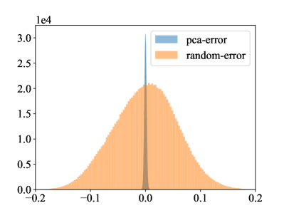
(a)

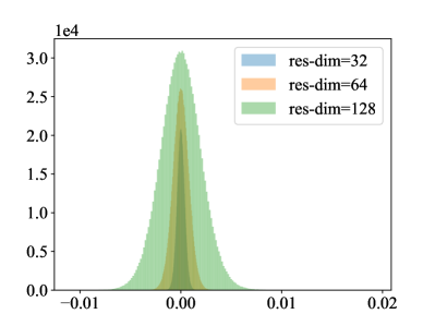
(b)

Figure 4. Example of PCA Error and Random Projection Error Distribution in Deep1M Dataset

4.2. More Informative Error Quantiles

Inspired by the role of error bounds in ADSampling, we introduce the concept of error quantiles. Compared to error bound, error quantiles contain more information, thus more likely to enable early determination whether a candidate point can be disregarded in the verification phase of AKNN search.

Base on the project distance decomposition we can get the following deterministic inequality

(3) $$\|\xx_{D}-\qq_{D}\|^{2}=C_{1}-C_{2}-2\cdot\Braket{\qq_{r},\xx_{r}}\geq C_{1}-C_{2}-2\cdot\|\qq_{r}\|\cdot\|\xx_{r}\|$$

The inequality is due to the Cauchy–Schwarz inequality, where

$$\Braket{\qq_{r},\xx_{r}}\leq\|\qq_{r}\|\cdot\|\xx_{r}\|$$

Remark. In fact, we can also apply the Hölder’s Inequality, which states that for $p$ and $q$ such that $\frac{1}{p}+\frac{1}{q}=1$.

Therefore, we have two choices:

$\bullet$ We can use the RHS of Equation (3) to prune candidates using $O(d)$ cost spent mainly to compute $\Braket{\qq_{d},\xx_{d}}$ (assuming the offline precomputed and loaded $\|\xx_{r}\|$ and $\|\xx_{d}\|$, on-the-fly and computed-once $\|\qq_{d}\|$ and $\|\qq_{r}\|$).

$\bullet$ Or, we can leverage a concentration inequality to prune the distance computation, akin to our focus on approximate nearest neighbor search.

Error Distribution. The Cauchy–Schwarz inequality achieves no false negative inequality. As we focus on the approximate nearest neighbor search, we can do better with the study of the distribution of the error which we set as $\epsilon=dis^{\prime}-dis$. With $O(d)$ computation, the approximate distance $dis^{\prime}=C_{1}-C_{2}$, the precise distance $dis=C_{1}-C_{2}-2\cdot\braket{\qq_{r},\xx_{r}}$ and the error $\epsilon=2\cdot\braket{\qq_{r},\xx_{r}}$. For $C_{1}$ part, The $\|\xx_{d}\|^{2}+\|\xx_{r}\|^{2}$ can precompute and store, the $\|\qq_{d}\|^{2}+\|\qq_{r}\|^{2}$ only need compute once for a single query. Remaining the $C_{2}$ part for $O(d)$ cost. As we mentioned before, we can leverage the variance of the error $\sigma_{e}^{2}=Var(-2\cdot\Braket{\qq_{r},\xx_{r}})$ and Chebyshev’s inequality to obtain a bound and utilize it to prune distance calculations as below:

$$P(|-2\cdot\Braket{\qq_{r},\xx_{r}}|\geq k\sigma_{e})\leq\frac{1}{k^{2}}$$

Or we can do better with the Gaussian distribution assumption.

Error Quantiles. Assume that the data follow the Gaussian distribution $\xx\sim\mathcal{N}(0,\Sigma)$. When query $\qq$ is given, the distribution of error can be regarded as a linear accumulation of multiple Gaussian distributions. Consider the error item $\epsilon=-2\cdot\Braket{\qq_{r},\xx_{r}}$ in Equation 2 of the $O(d)$ time complexity compute projection distance in a $d$-dimensional space. Since $\xx$ follows a zero mean, then for each dimension $x_{i}\sim\mathcal{N}(0,(\qq_{i}\sigma_{i})^{2})$ where $\sigma_{i}$ is the standard deviation in each dimension. Then we can get

(4) $$-2\cdot\Braket{\qq_{r},\xx_{r}}\sim\mathcal{N}(0,4\cdot\sum_{i=d+1}^{i\leq D}(\qq_{i}\sigma_{i})^{2}).$$

The variance of error only needs to be computed once for a single query $\qq$. Then we rewrite the distribution as $\epsilon\sim\mathcal{N}(0,\sigma^{2})$. From the empirical rule of Gaussian distribution, 99.7% of the values lie three standard deviations from the mean, which we can obtain an error quantile based on the accumulation of standard deviation($3\cdot\sigma$ for 99.7% quantile).

4.3. Implementaion

We then explore the integration of the projection method and the error quantiles into current AKNN algorithms, for utilization in the search process.

Deriving Data Distribution from Training Data. To minimize the residual dimension error and obtain the standard deviation of the error from the data distribution. We utilize training data with the same distribution to the queries for the generation of data distribution. Based on this distribution, we perform PCA projection and estimate the standard deviation of the residual dimensions. To get the distance bound, we employ the approximate distance $dis^{\prime}=C_{1}-C2$ minus $m$ times the error standard deviation, resulting in a high probability that the precise distance will be greater than the distance bound within the training data generate distribution. The entire process of ${\mathsf{BSA}}_{\text{res }}$is summarized in Algorithm  1. For the problem that the distribution of data changes under different search parameters, we perform PCA on the dataset points as an approximation. For the standard deviation, we can consider the KNN distribution of the query, because it will not change with the search parameters and directly affects search accuracy.

Input: Threshold $\tau$, Multiplier $m$, Project dim $d$, Transformed query $\qq$, Transformed data $\xx$

Output: Result: 0 with precise distance $dis$ or 1 with approximate distance $dis^{\prime}$

$C_{1}\leftarrow\|\xx\|^{2}+\|\qq\|^{2}$; // Precompute Once For Single Query

$C_{2}\leftarrow 2\cdot\Braket{\xx_{d},\qq_{d}}$; // Compute On the Fly

$\sigma_{r}\leftarrow\sqrt{4\cdot\Braket{\qq_{r}^{2},\sigma_{r}^{2}}}$; // Precompute Once For Single Query

1 if $C_{1}-C_{2}-m\cdot\sigma_{r}>\tau$ then

2       return 1 with $dis^{\prime}=(C_{1}-C_{2})$;

3      

4 end if

5else

       $C_{3}\leftarrow 2\cdot\Braket{\xx_{r},\qq_{r}}$; // Compute On the Fly

6       return 0 with $dis=(C_{1}-C_{2}-C_{3})$;

7      

8 end if

Algorithm 1 ${\mathsf{BSA}}_{\text{res }}$algorithm

Incremental Computation. A significant advantage of projection methods lies in the capability to compute the projection dimensions incrementally to achieve a more accurate approximation of distance up until the exact distance. Similar to ADSampling where sample projection dimensions are progressively increased ${\mathsf{BSA}}_{\text{res }}$also supports the incremental addition of computational dimensions. Specifically, for the current approximate distance $dis^{\prime}$, if ${\mathsf{BSA}}_{\text{res }}$prunes the computation of the exact distance for the current point, the computation halts. Conversely, if ${\mathsf{BSA}}_{\text{res }}$does not prune the precise distance computation for the current point, the computation proceeds by incrementally adding dimensions. Subsequently, the new approximate distance is utilized to continue pruning the precise computation until the accumulated dimensions reach the original dimensionality or it is pruned and stopped earlier. We summarize the method of using incremental ${\mathsf{BSA}}_{\text{res }}$in Algorithm 2.

Input: Threshold $\tau$, Multiplier $m$, Incremental Project dim $\Delta_{d}$, Transformed query $\qq$, Transformed data $\xx$

Output: Result: 0 with precise distance $dis$ or 1 with approximate distance $dis^{\prime}$

$C_{1}\leftarrow\|\xx\|^{2}+\|\qq\|^{2}$; // Precompute Once For Single Query

1

2while $d<D$ do

       $C_{2}\leftarrow C_{2}+2\cdot\Braket{\xx_{\Delta_{d}},\qq_{\Delta_{d}}}$; // Incremental Compute

3       $r\leftarrow D-d$;

       $\sigma_{r}\leftarrow\sqrt{4\cdot\Braket{\qq_{r}^{2},\sigma_{r}^{2}}}$; // Load Precompute Variance

4       if $C_{1}-C_{2}-m\cdot\sigma_{r}>\tau$ then

5             return 1 with $dis^{\prime}=(C_{1}-C_{2})$;

6            

7       end if

8      else

9             $d\leftarrow d+\Delta_{d}$;

10            

11       end if

12      

13 end while

Algorithm 2 Incremental-${\mathsf{BSA}}_{\text{res }}$

5. A General Distance Computation Method

This section mainly addresses the lack of generality associated with ADSampling. Follow the same idea as from ${\mathsf{BSA}}_{\text{res }}$of using training data to get a distance quantile for pruning the distance computation. We propose the quantile-driven framework that ${\mathsf{BSA}}_{\text{res }}$can be regarded as an instance of it. Building on this foundation, we propose a learning-based approach as a new instance that is applicable to various approximate distances and offers parameter selection tailored to different AKNN search precision requirements. Note that our method does not impose any requirements on how to obtain approximate distances, which allows for broader applicability compared to ADSampling.

5.1. Quantile-Driven Framework

We encapsulate the core idea of the ${\mathsf{BSA}}_{\text{res }}$algorithm in Section 4 within a quantile-driven framework. The essence of this approach lies in leveraging a training set that shares the distribution with the queries to obtain the error distribution of approximate distances during the querying process. Subsequently, the approximate distance minus the upper quantile of the error is used as the distance bound to prune distance computations. We summarize it as the $\mathsf{BSA}$ framework, as shown in Figure 5.

Figure 5. The Process of Quantile-Driven Framework

The $\mathsf{BSA}$ framework is utilized to determine the distribution of this error by calculating both the precise and approximate distances. Training data with a distribution analogous to the query is used to generate the search data distribution. To determine the error quantile, the ${\mathsf{BSA}}_{\text{res }}$instance uses the multiplier and the standard deviation of the error to get the error quantile $\epsilon_{q}$. Given the error quantile $\epsilon_{q}$, the inequality $dis>dis^{\prime}-\epsilon_{q}$ ensures a manageable probability of error occurrence in the training data. Thus, the criterion $dis^{\prime}-\epsilon_{q}>\tau$ can be utilized to determine whether reliance on the approximate distance is adequate or if a precise distance computation is required.

5.2. A Learning-Based Instance

The ${\mathsf{BSA}}_{\text{res }}$approach aims to minimize the error quantile, thereby improving the query efficiency. However, the ${\mathsf{BSA}}_{\text{res }}$approach cannot be easily adjusted to other approximate distances, since it is difficult to guarantee that the error follows the Gaussian distribution. Meanwhile, ${\mathsf{BSA}}_{\text{res }}$still needs to manually set the standard deviation multiplier to meet the AKNN’s accuracy requirement. Therefore, in this section, our objective is to solve these two problems with the learned-based method, which can easily adapt to any approximate distance and provide auto parameter configuration for any search accuracy requirement.

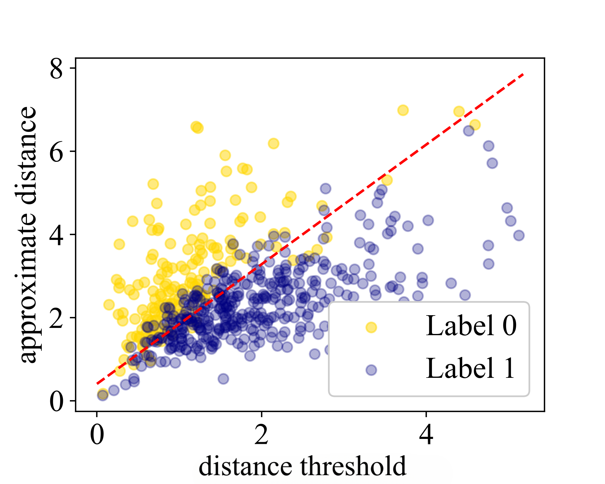
(a)

(b)

(c)

(d)

Figure 6. Example of Linear Models with PCA as Approximate Distance

For the generation of training data, we still follow the same process as with the ${\mathsf{BSA}}_{\text{res }}$instance, but since we consider arbitrary approximate distances, we cannot rely solely on projection methods to minimize error. Instead, we use a linear model to replace the minimization of errors. Specifically, we use features related to the approximate distance to reconstruct the precise distance, achieving higher pruning efficiency. To achieve an efficient classifier, we use the approximate distance $dis^{\prime}$ and the threshold $\tau$ as features, and then we learn the weight of two features and the intercept that can be used to classify whether $dis$ is greater than $\tau$. The linear model can be written as:

$$L =sign(w_{1}dis^{\prime}+w_{2}\tau+b>0)$$

$$=sign(m_{1}dis^{\prime}+\beta>\tau)$$

where Label 0: $dis\leq\tau$ and Label 1: $dis>\tau$. We employ a straightforward linear model with Binary Cross-Entropy (BCE) as the loss function to implement our model. From our practical experiments and experience, using BCE as the reconstruction loss results in a more stable performance compared to other linear reconstruction methods, such as using Least Squares to minimize the MSE (Mean Squared Error) of distance approximation.

With the reconstruction distance $m_{1}dis^{\prime}+\beta$, we can use the numerical method such as binary search for the intercept term $\beta^{\prime}$(work same as error quantile) to ensure $dis>m_{1}dis^{\prime}+\beta^{\prime}$ with a manageable small failure probability. However, the failure probability of equation $dis>m_{1}dis^{\prime}+\beta^{\prime}$ cannot directly affect search accuracy. We are expected to obtain the $\beta^{\prime}$ corresponding to the recall target for a specific AKNN search accuracy. As we take the BCE as the loss function, we can set the threshold $\tau$ as the $k$-NN distance of query where Label 0 data becomes the KNN of query. Then we can binary search $\beta^{\prime}$ to ensure that the learned instance achieves the target recall $r$ on Label 0 in the training dataset to achieve auto parameter configuration.

Remark. The learning-based instance is comparable to the ${\mathsf{BSA}}_{\text{res }}$approach of Section 4 by taking $m_{1}=1$ and $\beta=m\cdot\sigma$. The difference is that the learned-based method is capable of any approximate distance which is more general.

5.3. Implementation

Approximate Distance and Feature Select. For projection-based approximate distance, we use the simple PCA projection as the approximate distance without taking the decomposition by Equation 2 for the general case denoted as ${\mathsf{BSA}}_{\text{pca }}$. For another popular approximate method, the product quantization distance, we utilize the distance to quantized centroids of the query $q$ to the database point $u$ known as the Asymmetric Distance Computation (ADC), as the approximate distance $dis^{\prime}$. Following the same idea as PCA, we use OPQ (Ge et al., 2014) as our final quantized approximate distance method, which also uses an orthogonal matrix to rotate the space for a more precise approximate distance and denote as ${\mathsf{BSA}}_{\text{opq }}$. More accurate quantification methods, such as AQ (Babenko and Lempitsky, 2014), CompQ (Zhang et al., 2014), LSQ (Martinez et al., 2018), and other additional quantification methods are no longer within the scope of our consideration due to their low efficiency of the lookup table. For quantization methods, we can also utilize the distance from $u$ itself to the quantized centroid as an additional feature. This multi-feature approach can further enhance the effectiveness of the linear model. Moreover, we noticed that product quantization has different optimizations with different hardware environments. In our experiments, we additionally analyzed the inference efficiency of using the PQ-scan(André et al., 2015) as an approximate distance with the SIMD-SSE instruction.

Multiple Linear Model. We can also use multiple linear models with the same idea in ADSampling or Algorithm 2, denoted as $L_{1},..,L_{n}$, each corresponding to a unique projection dimension as shown in figure 6, with an associated error probability $e_{1},..,e_{n}$ on Label 0 classification. If the $dis^{\prime}$ for the current projection dimension is classified as Label 0 by the current linear model $L_{i}$, we continue to increase the projection dimension. This process continues until the project dimension equals the original dimension, at which point we obtain an accurate distance. If this distance is less than the threshold $\tau$, we update the result queue.

To achieve the target recall $r$ for Label 0, we need to consider the number of false positives (FP) for each linear model. A straightforward strategy is to set the recall target for each of the $n$ linear models as $r_{i}=(1-(1-r)/n)$. This approach ensures that the overall recall target still satisfies the recall constraint for label 0. With the same idea as ADSampling, we also set a corresponding classifier $L_{i}$ for every $\Delta_{d}$ dimension. At the same time, the target recall for each classifier is set as $r_{i}=(1-(1-r)/(D/\Delta_{d}))$. If the current classifier result is 0, we continue to calculate the projection distance and use the next classifier until the exact distance is computed. Otherwise, we prune this candidate. It is worth noting that we do not use multiple linear classifiers with ${\mathsf{BSA}}_{\text{opq }}$. This is because of the use case of SIMD Instruction, which computes 4 or 8 quantized distances in one operation. Early stopping of one quantized distance will not improve performance unless all quantized distances stop early.

6. Time and Space Analysis

6.1. Projection Distance

We first study the time complexity of the ${\mathsf{BSA}}_{\text{res }}$and ${\mathsf{BSA}}_{\text{pca }}$based on the PCA projection. For the case without incremental computation, the expected time complexity of a single inference is highly dependent on the pruning rate, the ratio of the pruned cases to all distance comparison operations. For PCA as an approximate distance, as the projection dimension is $d$ and the pruning rate $\eta$ with the corresponding ${\mathsf{BSA}}_{\text{pca }}$instance. The expected time complexity of a single inference is $O(d\cdot\eta+(D-d)\cdot(1-\eta))$. Another benefit of the projection distance is that the project process can be regarded as rotating the space, and we can continue to add dimensions until we obtain the precise distance. This approach does not require extra space usage and reuses the approximate distance, potentially enhancing efficiency. The ${\mathsf{BSA}}_{\text{res }}$and ${\mathsf{BSA}}_{\text{pca }}$methods introduce additional time for rotating the space. For a single query, we require a time complexity of $O(D^{2})$ to perform matrix multiplication to project (rotate) the query. Furthermore, for the ${\mathsf{BSA}}_{\text{res }}$method, we incur an extra time cost of $O(D)$ to calculate the variance of the residual dimension by accumulating the product of the variance of each dimension and the corresponding query dimension. We also need $O(D)$ time to compute the square sum of query $q$. For the ${\mathsf{BSA}}_{\text{res }}$method, we further require an additional $O(n)$ space to store the square of the square sum of each vector.

Then we consider the multi-linear model with the PCA method. Assume that we have $m$ linear models with every $\Delta_{d}\cdot m=D$ for each linear model. The pruning rate for each linear model is denoted by $\eta_{1},..\eta_{m}$. Then the expected time complexity for a single inference is the following.

$$O(\sum\limits_{i\leq m}^{i=1}i\cdot\Delta_{d}\cdot\prod\limits_{j<i}^{j=1}(1-\eta_{j})\cdot\eta_{i})$$

Calculating the above time complexity can also be regarded as calculating the average scan dimension.

6.2. Quantization Distance

For the quantization method, as OPQ in our approach, the additional time cost consists of both the query rotation $O(D^{2})$ and the construction of a lookup table. With OPQ implemented across $m$ subspaces, each containing $2^{nbit}$ quantized centroid, the time complexity of constructing a look-up table is $O(D\cdot 2^{nbit})$. With the look-up table, the calculation of the asymmetric distance requires only $m$ times the look-up from the table. Unlike the projection method, the quantized-based approach needs to recompute the distance if it cannot prune the precise distance computation, rather than increment the cumulative dimension. With the linear model $L$ and the pruning rate $\eta_{q}$, the expected time complexity for single inference is $O(m+(1-\eta_{q})\cdot D)$. The features of the linear model $L$ are the approximate distance, the point-to-centroid distance, and the threshold. Differing from the projection-based method, the use of quantization brings extra space costs. Considering quantization across $m$ subspaces, the extra space cost requires $n\cdot m\cdot nbit$ bits. Where the $m$ is usually taken as $1/4$ or $1/8$ of origin dimension $D$ and the extra space cost is from $1/32$ to $1/64$ of the dataset’s size when using 32-bit float vectors.

7. Experiments

7.1. Experimental Settings

Datasets. We employ six publicly available datasets of different sizes and dimensionalities, as outlined in Table 2. These datasets have been extensively utilized as benchmarks for evaluating AKNN search algorithms. It is important to note that these publicly available datasets encompass base vectors and query vectors. For datasets that provide learning data, such as GIST and DEEP, we directly utilize the provided learning data. However, for datasets that do not provide learning data, we randomly sample 100,000 instances from the base data to train the linear model and then remove them from the base data. Note that all vector data in the experiment are stored in float32 format.

Table 2. Dataset Statistics

Dataset	Dimension	Size	Query Size
SIFT	128	10,000,000	1000
GIST	960	1,000,000	1000
DEEP	256	1,000,000	1000
GLOVE	300	2,196,017	1000
TINY5M	384	5,000,000	1000
WORD2VEC	300	1,000,000	1000

(a)

(b)

(c)

(d)

(e)

(f)

(g)

(h)

(i)

(j)

(k)

(l)

(m)

(n)

(o)

(p)

(q)

(r)

(s)

(t)

(u)

(v)

(w)

(x)

Figure 7. Time-Accuracy Tradeoff and Dimensionality (HNSW and IVF)

Performance Evaluation. We employ recall as a metric, quantifying the ratio of successfully retrieved ground truth $k$-nearest neighbors to the total number of $k$ neighbors. To gauge efficiency, we utilize query-per-second (QPS), which measures the number of queries processed per second, including the end-to-end query time, product quantization codebook calculation time, and encompassing random transformations on query vectors. Additionally, we evaluate the total number of dimensions scanned by random projection and PCA. For OPQ we use the pruning rate to evaluate the efficiency. All the metrics mentioned are averaged over the entire query set.

Compare Method. We list the compared method below:

• ${\mathsf{HNSW}}$: ${\mathsf{HNSW}}$ with all precise distances computed.

• ${\mathsf{HNSW}}$++: ${\mathsf{HNSW}}$ with ADSampling method.

• ${\mathsf{HNSW}}$-${\mathsf{BSA}}_{\text{opq }}$: ${\mathsf{HNSW}}$ takes OPQ as the approximate distance for the learned instance approach.

• ${\mathsf{HNSW}}$-${\mathsf{BSA}}_{\text{pca }}$: ${\mathsf{HNSW}}$ takes PCA as the approximate distance for the learned instance approach.

• ${\mathsf{HNSW}}$-${\mathsf{BSA}}_{\text{res }}$: ${\mathsf{HNSW}}$ takes residual dimension variance for pruning.

• ${\mathsf{IVF}}$: ${\mathsf{IVF}}$ with all precise distances computed.

• ${\mathsf{IVF}}$++: ${\mathsf{IVF}}$ with ADSampling method.

• ${\mathsf{IVF}}$-${\mathsf{BSA}}_{\text{opq }}$: ${\mathsf{IVF}}$ takes OPQ as the approximate distance for the learned instance approach.

• ${\mathsf{IVF}}$-${\mathsf{BSA}}_{\text{pca }}$: ${\mathsf{IVF}}$ takes PCA as the approximate distance for the learned instance approach.

• ${\mathsf{IVF}}$-${\mathsf{BSA}}_{\text{res }}$: ${\mathsf{IVF}}$ takes residual dimension variance for pruning.

Training Configuration. For the training of the linear models, we directly take the KNN of learning data as label 0. For data with label 1, we treat the learning data as the query and generate training data by recording the visited points and eliminating the KNN(label 0). For all training items, we compute their approximate distance, threshold, and other features to train the linear classifier with BCE as the loss. Specifically, we use 10,000 learning vector data for each dataset as training queries and perform the search algorithm with a fixed configuration to get the training data. For the search parameters used to generate label 1 data, we empirically tune it so that it can generate enough label 1 data. Our experiments also show that, as long as the scale of label 1 is sufficient, the model demonstrates good generalization across different search parameters. We set the recall target $r$ as 0.995 for the time-accuracy tradeoff experiment and provide a verified recall target experiment as follows.

Index Configuration. We mainly consider the index construction of two AKNN algorithms, ${\mathsf{HNSW}}$, and ${\mathsf{IVF}}$. For ${\mathsf{HNSW}}$, two key parameters control the graph construction: $M$ determines the number of connected neighbors, and $efConstruction$ controls the quality of the approximate nearest neighbors. Following the original ${\mathsf{HNSW}}$ work, we set $M=16$ and $efConstruction=500$. For ${\mathsf{IVF}}$, as recommended in the Faiss library, the number of clusters should be around the square root of the database size. We set the number of clusters to 4,096 as in ADSampling. All C++ code compiles with g++ 11.4.0 and -O3 optimization. Python code (used in indexing and training for linear models, PCA, and OPQ) runs on Python 3.8. Experiments use an Intel(R) Xeon(R) Platinum 8352V CPU @ 2.10GHz with 512GB memory, running in Ubuntu Linux. We present results with SSE in (Yang et al., 2024) due to space limit.

Approximate Distance Configuration. For the random projection approach, we set $\epsilon_{0}=2.1$ and $\Delta_{d}=32$ which is recommended as the best performance in ADSampling. For the PCA approach, we also set every $\Delta_{d}=32$ dimension to construct a linear model to achieve the same condition as ADSampling. For the OPQ approach, we set the subspace number as $d/8$ for the GIST dataset and $d/4$ for the others since all the dimensions of the dataset can be divided by 4. The features used for the PCA approach are the project distance(approximate distance) and the threshold. For the OPQ approach, we added an additional point-to-centroid distance as a feature. The target recall is set as 0.995 for the ${\mathsf{BSA}}_{\text{pca }}$and ${\mathsf{BSA}}_{\text{opq }}$methods. For the multiplier $m$ for ${\mathsf{BSA}}_{\text{res }}$, we set it as 8 for SIFT, GIST, and DEEP, 12 for TINY and WORD2VEC, and 16 for the GlOVE dataset. For the case of multiple classifiers, we set the target recall for each classifier based on $\Delta_{d}$ as $r_{i}=(1-(1-r)/(D/\Delta_{d}))$.

7.2. Experimental Results

Overall Results. We plot the time accuracy curve with two popular algorithms $\mathsf{HNSW}$ and $\mathsf{IVF}$ which the upper right is better. We denote that the method ${\mathsf{HNSW}}$++ is the ADSampling method with the $k$-size result queue threshold as illustrated in the figure 7. We use ${\mathsf{HNSW}}$-${\mathsf{BSA}}_{\text{res }}$, ${\mathsf{HNSW}}$-${\mathsf{BSA}}_{\text{pca }}$and ${\mathsf{HNSW}}$-${\mathsf{BSA}}_{\text{opq }}$to represent the ${\mathsf{HNSW}}$ with a residual-based classifier, a learned-based classifier with PCA and OPQ as an approximate distance feature. We also adapt the split result queue strategy in ${\mathsf{HNSW}}$++. The ${\mathsf{IVF}}$++ denotes the ADSampling method with cache level optimization, and ${\mathsf{IVF}}$-${\mathsf{BSA}}_{\text{pca }}$represents the PCA approximate method with the same optimization as ${\mathsf{IVF}}$++. The ${\mathsf{IVF}}$-${\mathsf{BSA}}_{\text{opq }}$method represents the OPQ approximate method without any cache-level optimization, but we provide experiments with SIMD instructors implemented in the Appendix.

To achieve the tradeoff between time-accuracy, we varying $N^{ef}$ for ${\mathsf{HNSW}}$, ${\mathsf{HNSW}}$++, ${\mathsf{HNSW}}$-${\mathsf{BSA}}_{\text{opq }}$, ${\mathsf{HNSW}}$-${\mathsf{BSA}}_{\text{pca }}$, ${\mathsf{HNSW}}$-${\mathsf{BSA}}_{\text{res }}$and $N^{probe}$ for ${\mathsf{IVF}}$, ${\mathsf{IVF}}$++, ${\mathsf{IVF}}$-${\mathsf{BSA}}_{\text{opq }}$, ${\mathsf{IVF}}$-${\mathsf{BSA}}_{\text{pca }}$, ${\mathsf{IVF}}$-${\mathsf{BSA}}_{\text{res }}$. As the focus of our approach, we consider the high recall($>85\%$) as the main scenario that the approximate distance methods without fast inference cannot achieve. We observe the following results. (1) From the overall experimental result, the fast inference method can achieve a large margin speed-up with the ${\mathsf{IVF}}$-based method in which DCOs constitute the main time cost. (2) For the WORD2VEC dataset with the ${\mathsf{HNSW}}$ method, the recall reaches a bottleneck at $85\%$(caused by outdegree limitation of ${\mathsf{HNSW}}$) and the performance of all fast inference methods including ADSampling has a significant discrepancy compared with other datasets. For ${\mathsf{HNSW}}$+, ${\mathsf{IVF}}$+, and PDScanning methods proposed by ADSampling, that is, methods that do not use split queues, memory layout optimization, and the incremental distance calculation with the threshold. The performance of the above methods has a significant gap compared to ${\mathsf{HNSW}}$++ and ${\mathsf{IVF}}$++, which are no longer considered in our experiment.

(a)

(b)

(c)

(d)

Figure 8. Parameter Study on Target Recall $\tau$

Results of Verified Target Recall. We study the parameter of target recall with different approximate methods. As we mentioned in the preliminary, the actual threshold is greater than the threshold for training. Therefore, target recall is the expected lower bound on training data. The overall performance of the recall will be better than the target recall since the update threshold will be larger than the ground truth threshold(we take the current threshold as the feature for inference). Moreover, for multiple linear models, we use the same strategy as union-bound, which will also make the test recall higher than the target. As in the parameter study of $r$ in Fig. 8, we found that in the case of $r=0.995$, the search algorithm of both ${\mathsf{IVF}}$ and ${\mathsf{HNSW}}$ can achieve the best tradeoff between efficiency and recall loss(less than 0.5%) which is selected as the default target recall.

Results of Extra Time. A common aspect of ADsampling and our approach is the transformation of vector data, which incurs additional time costs. Upon receiving a query, the search algorithm first executes the transformation, and its cost can be amortized by all the distance computations involved in answering the same query. We implement this process via a matrix multiplication operation(with C++ Eigen Library), which takes $O(D^{2})$ time and 0.344ms with GIST data. Moreover, the OPQ inference requires additional time cost for the computation of the look-up table, which takes $O(2^{nbit}\cdot D)$ time and can be considered as $2^{nbit}$ times (usually 256) distance calculation, which takes 0.170ms with GIST data. The ratio between the extra time and the full query time is illustrated in Table 3.

$N^{ef}$	Proj	PCA	OPQ
500	6.0%	8.9%	12% + 5.9%
1000	3.9%	5.6%	7.6% + 3.8%
1500	3.0%	3.1%	5.8% + 2.9%
2000	2.5%	2.9%	4.7% + 2.3%

Table 3. Extra Time Ratio on GIST-HNSW

Results of Scan Dimensions. The ADSampling method and the PCA inference method can be evaluated by the scan dimensions since the visited point set is the same. We plot the average scan dimension ratio compared with the naive method plot(red line) to the ADSampling method(orange line) and ${\mathsf{BSA}}_{\text{pca }}$method(green line) with the left axis in figure 9. For the ${\mathsf{BSA}}_{\text{opq }}$method, we plot the pruning rate with the right axis and blue line to verify its efficiency. The query performance corresponds to the time-accuracy tradeoff in Figure 7. It can be observed that the ratio of average scan dimension decreased as the search algorithm visited more points(with larger search parameters). With a larger search parameter, the OPQ with 120 subspaces(for the GIST dataset) inference can achieve a near 100%($\geq$95%) pruning rate which means that the case of needed full precise data only consists of a very small portion. This observation can make our approach more suitable to combine with disk-based methods.

Figure 9. Dimension Scan Rate and Pruned Rate

Results for Evaluating the Distance Approximation. We then study the method with only approximate distances without error quantile or bound. We take the OPQ with HNSW and IVF algorithms notes as ${\mathsf{HNSW}}_{\text{opq}}$ and ${\mathsf{IVF}}_{\text{opq}}$. The approximate distance method with the parameter 120 subspaces for the GIST dataset and 64 subspaces for the DEEP dataset is the same parameters as ${\mathsf{HNSW}}$-${\mathsf{BSA}}_{\text{opq }}$and ${\mathsf{HNSW}}$-${\mathsf{BSA}}_{\text{opq }}$. It can be seen that there is about a 7% to 9% recall gap between the OPQ-only method(${\mathsf{HNSW}}_{\text{opq}}$, ${\mathsf{IVF}}_{\text{opq}}$) to the leaned inference one. The approximate distance with PCA at the same setting will become even worse as the OPQ is more accurate than PCA in various data settings.

(a)

(b)

Figure 10. Recall@1 Time-Accuracy Tradeoff

8. Related Work

8.1. Existing AKNN Algorithms

Existing methods for accelerating the computation of distances between points/vectors include ADSampling(Gao and Long, 2023) and FINGER(Chen et al., 2023). ADSampling relies on the Johnson-Lindenstrauss (JL) lemma(Johnson et al., 1986) to provide a probabilistic bound and uses it to accelerate distance calculations. FINGER(Chen et al., 2023), on the other hand, is a method applicable solely to graph-based approaches, primarily by estimating angles between neighboring residual vectors during the graph search stage to achieve acceleration. FINGER is exclusively applied to graph-based methods and is therefore not included in the baseline comparison.

8.2. Learning-Based Methods for AKNN search

Learning-based methods have made significant contributions to the field of graph-based AKNN search. Notably, several recent studies have leveraged machine learning techniques to enhance different aspects of AKNN search. In particular, (Baranchuk et al., 2019; Feng et al., 2023) have applied learning techniques to predict the next node during graph traversal, enabling more efficient navigation through the search space.

It is important to note that the majority of these learning-based approaches primarily focus on improving the index construction and search processes of AKNN search. They often overlook the critical aspect of distance calculation, which constitutes a significant portion of the overall search time. In contrast, our approach places a strong emphasis on distance computation, enabling seamless integration with the aforementioned methods. By tackling the computational bottlenecks inherent in distance calculations, our method provides a comprehensive solution to boost AKNN search efficiency throughout the search process.

9. Conclusion

In this paper, we present an innovative approach that significantly improves both the accuracy and efficiency of AKNN search. Our proposed methodology revolves around decomposing the computation of projection distances, optimizing the projection matrix to minimize error terms, and employing an error quantile to effectively prune unnecessary distance computations. Moreover, through a quantile-driven framework that utilizes learning-based methods and numerical analysis, our approach demonstrates notable improvements in search speed over the current method ADSampling, especially on datasets of different data types and scales.

In addition, it is necessary to consider similarities beyond Euclidean Space. (1) The cosine-based similarity and inner product similarity search on given data and query vectors is equivalent to the Euclidean nearest neighbor search on their normalized data and query vectors. (2) Otherwise we can directly use the corresponding approximate method such as the product quantization in inner product space (Guo et al., 2016, 2020) for quantization distances with relatively low quantization distortion and computation cost. With the more accurate approximate method, our approach can achieve a higher efficiency improvement with the accuracy requirement constraint.

References

- (1)
- André et al. (2015) Fabien André, Anne-Marie Kermarrec, and Nicolas Le Scouarnec. 2015. Cache locality is not enough: High-Performance Nearest Neighbor Search with Product Quantization Fast Scan. Proceedings of the VLDB Endowment 9, 4 (2015).
- Babenko and Lempitsky (2014) Artem Babenko and Victor Lempitsky. 2014. Additive quantization for extreme vector compression. In Proceedings of the IEEE Conference on Computer Vision and Pattern Recognition (CVPR). 931–938.
- Babenko and Lempitsky (2015) Artem Babenko and Victor S. Lempitsky. 2015. The Inverted Multi-Index. IEEE Trans. Pattern Anal. Mach. Intell. 37, 6 (2015), 1247–1260.
- Baranchuk et al. (2019) Dmitry Baranchuk, Dmitry Persiyanov, Anton Sinitsin, and Artem Babenko. 2019. Learning to route in similarity graphs. In International Conference on Machine Learning. PMLR, 475–484.
- Beygelzimer et al. (2006) Alina Beygelzimer, Sham Kakade, and John Langford. 2006. Cover trees for nearest neighbor. In Proceedings of the 23rd international conference on Machine learning. 97–104.
- Chen et al. (2023) Patrick Chen, Wei-Cheng Chang, Jyun-Yu Jiang, Hsiang-Fu Yu, Inderjit Dhillon, and Cho-Jui Hsieh. 2023. FINGER: Fast Inference for Graph-based Approximate Nearest Neighbor Search. In Proceedings of the ACM Web Conference 2023. 3225–3235.
- Cover and Hart (1967) Thomas Cover and Peter Hart. 1967. Nearest neighbor pattern classification. IEEE transactions on information theory 13, 1 (1967), 21–27.
- Dasgupta and Freund (2008) Sanjoy Dasgupta and Yoav Freund. 2008. Random projection trees and low dimensional manifolds. In Proceedings of the fortieth annual ACM symposium on Theory of computing. 537–546.
- Feng et al. (2023) Chao Feng, Defu Lian, Xiting Wang, Zheng Liu, Xing Xie, and Enhong Chen. 2023. Reinforcement routing on proximity graph for efficient recommendation. ACM Transactions on Information Systems 41, 1 (2023), 1–27.
- Fu et al. (2022) Cong Fu, Changxu Wang, and Deng Cai. 2022. High Dimensional Similarity Search With Satellite System Graph: Efficiency, Scalability, and Unindexed Query Compatibility. IEEE Trans. Pattern Anal. Mach. Intell. 44, 8 (2022), 4139–4150.
- Fu et al. (2019) Cong Fu, Chao Xiang, Changxu Wang, and Deng Cai. 2019. Fast Approximate Nearest Neighbor Search With The Navigating Spreading-out Graph. Proc. VLDB Endow. 12, 5 (2019), 461–474.
- Gan et al. (2012) Junhao Gan, Jianlin Feng, Qiong Fang, and Wilfred Ng. 2012. Locality-sensitive hashing scheme based on dynamic collision counting. In Proceedings of the 2012 ACM SIGMOD international conference on management of data. 541–552.
- Gao and Long (2023) Jianyang Gao and Cheng Long. 2023. High-Dimensional Approximate Nearest Neighbor Search: with Reliable and Efficient Distance Comparison Operations. Proc. ACM Manag. Data 1, 2 (2023), 137:1–137:27. https://doi.org/10.1145/3589282
- Ge et al. (2014) Tiezheng Ge, Kaiming He, Qifa Ke, and Jian Sun. 2014. Optimized Product Quantization. IEEE Trans. Pattern Anal. Mach. Intell. 36, 4 (2014), 744–755.
- Goemans and Williamson (1995) Michel X Goemans and David P Williamson. 1995. Improved approximation algorithms for maximum cut and satisfiability problems using semidefinite programming. Journal of the ACM (JACM) 42, 6 (1995), 1115–1145.
- Guo et al. (2016) Ruiqi Guo, Sanjiv Kumar, Krzysztof Choromanski, and David Simcha. 2016. Quantization based fast inner product search. In Artificial intelligence and statistics. PMLR, 482–490.
- Guo et al. (2020) Ruiqi Guo, Philip Sun, Erik Lindgren, Quan Geng, David Simcha, Felix Chern, and Sanjiv Kumar. 2020. Accelerating large-scale inference with anisotropic vector quantization. In International Conference on Machine Learning. PMLR, 3887–3896.
- Harwood and Drummond (2016) Ben Harwood and Tom Drummond. 2016. Fanng: Fast approximate nearest neighbour graphs. In Proceedings of the IEEE Conference on Computer Vision and Pattern Recognition. 5713–5722.
- Huang et al. (2017) Qiang Huang, Jianlin Feng, Qiong Fang, Wilfred Ng, and Wei Wang. 2017. Query-aware locality-sensitive hashing scheme for lp norm. The VLDB Journal 26, 5 (2017), 683–708.
- Huang et al. (2015) Qiang Huang, Jianlin Feng, Yikai Zhang, Qiong Fang, and Wilfred Ng. 2015. Query-aware locality-sensitive hashing for approximate nearest neighbor search. Proceedings of the VLDB Endowment 9, 1 (2015), 1–12.
- Indyk and Motwani (1998) Piotr Indyk and Rajeev Motwani. 1998. Approximate nearest neighbors: towards removing the curse of dimensionality. In Proceedings of the thirtieth annual ACM symposium on Theory of computing. 604–613.
- Jégou et al. (2011) Hervé Jégou, Matthijs Douze, and Cordelia Schmid. 2011. Product Quantization for Nearest Neighbor Search. IEEE Trans. Pattern Anal. Mach. Intell. 33, 1 (2011), 117–128.
- Johnson et al. (1986) William B Johnson, Joram Lindenstrauss, and Gideon Schechtman. 1986. Extensions of Lipschitz maps into Banach spaces. Israel Journal of Mathematics 54, 2 (1986), 129–138.
- Lewis et al. (2020) Patrick Lewis, Ethan Perez, Aleksandra Piktus, Fabio Petroni, Vladimir Karpukhin, Naman Goyal, Heinrich Küttler, Mike Lewis, Wen-tau Yih, Tim Rocktäschel, et al. 2020. Retrieval-augmented generation for knowledge-intensive nlp tasks. Advances in Neural Information Processing Systems 33 (2020), 9459–9474.
- Li et al. (2020) Wen Li, Ying Zhang, Yifang Sun, Wei Wang, Mingjie Li, Wenjie Zhang, and Xuemin Lin. 2020. Approximate Nearest Neighbor Search on High Dimensional Data - Experiments, Analyses, and Improvement. IEEE Trans. Knowl. Data Eng. 32, 8 (2020), 1475–1488.
- Liu et al. (2007) Ying Liu, Dengsheng Zhang, Guojun Lu, and Wei-Ying Ma. 2007. A survey of content-based image retrieval with high-level semantics. Pattern recognition 40, 1 (2007), 262–282.
- Lu et al. (2021) Kejing Lu, Mineichi Kudo, Chuan Xiao, and Yoshiharu Ishikawa. 2021. HVS: Hierarchical Graph Structure Based on Voronoi Diagrams for Solving Approximate Nearest Neighbor Search. Proc. VLDB Endow. 15, 2 (2021), 246–258.
- Malkov et al. (2014) Yury Malkov, Alexander Ponomarenko, Andrey Logvinov, and Vladimir Krylov. 2014. Approximate nearest neighbor algorithm based on navigable small world graphs. Inf. Syst. 45 (2014), 61–68.
- Malkov and Yashunin (2020) Yury A. Malkov and Dmitry A. Yashunin. 2020. Efficient and Robust Approximate Nearest Neighbor Search Using Hierarchical Navigable Small World Graphs. IEEE Trans. Pattern Anal. Mach. Intell. 42, 4 (2020), 824–836.
- Martinez et al. (2018) Julieta Martinez, Shobhit Zakhmi, Holger H. Hoos, and James J. Little. 2018. LSQ++: Lower running time and higher recall in multi-codebook quantization. In Proceedings of the European Conference on Computer Vision (ECCV).
- Peng et al. (2023) Yun Peng, Byron Choi, Tsz Nam Chan, Jianye Yang, and Jianliang Xu. 2023. Efficient Approximate Nearest Neighbor Search in Multi-dimensional Databases. Proc. ACM Manag. Data 1, 1 (2023), 54:1–54:27. https://doi.org/10.1145/3588908
- Ram and Sinha (2019) Parikshit Ram and Kaushik Sinha. 2019. Revisiting kd-tree for nearest neighbor search. In Proceedings of the 25th acm sigkdd international conference on knowledge discovery & data mining. 1378–1388.
- Schafer et al. ([n.d.]) J Ben Schafer, Dan Frankowski, Jon Herlocker, and Shilad Sen. [n.d.]. Collaborative filtering recommender systems. In The adaptive web: methods and strategies of web personalization. Springer, 291–324.
- Sun et al. (2014) Yifang Sun, Wei Wang, Jianbin Qin, Ying Zhang, and Xuemin Lin. 2014. SRS: Solving c-Approximate Nearest Neighbor Queries in High Dimensional Euclidean Space with a Tiny Index. Proc. VLDB Endow. 8, 1 (2014), 1–12.
- Yang et al. (2024) Mingyu Yang, Jiabao Jin, Xiangyu Wang, Zhitao Shen, Wei Jia, Wentao Li, and Wei Wang. 2024. Technical Report. https://github.com/mingyu-hkustgz/Res-Infer/blob/nolearn/Technical%20Report.pdf
- Zhang et al. (2014) Ting Zhang, Chao Du, and Jingdong Wang. 2014. Composite quantization for approximate nearest neighbor search. In International Conference on Machine Learning. PMLR, 838–846.
- Zheng et al. (2020) Bolong Zheng, Xi Zhao, Lianggui Weng, Nguyen Quoc Viet Hung, Hang Liu, and Christian S. Jensen. 2020. PM-LSH: A Fast and Accurate LSH Framework for High-Dimensional Approximate NN Search. Proc. VLDB Endow. 13, 5 (2020), 643–655.