Parallel and (Nearly) Work-Efficient Dynamic Programming

Abstract.

The idea of dynamic programming (DP), proposed by Bellman in the 1950s, is one of the most important algorithmic techniques. However, in parallel, many fundamental and sequentially simple problems become more challenging, and open to a (nearly) work-efficient solution (i.e., the work is off by at most a polylogarithmic factor over the best sequential solution). In fact, sequential DP algorithms employ many advanced optimizations such as decision monotonicity or special data structures, and achieve better work than straightforward solutions. Many such optimizations are inherently sequential, which creates extra challenges for a parallel algorithm to achieve the same work bound.

The goal of this paper is to achieve (nearly) work-efficient parallel DP algorithms by parallelizing classic, highly-optimized and practical sequential algorithms. We show a general framework called the Cordon Algorithm for parallel DP algorithms, and use it to solve several classic problems. Our selection of problems includes Longest Increasing Subsequence (LIS), sparse Longest Common Subsequence (LCS), convex/concave generalized Least Weight Subsequence (LWS), Optimal Alphabetic Tree (OAT), and more. We show how the Cordon Algorithm can be used to achieve the same level of optimization as the sequential algorithms, and achieve good parallelism. Many of our algorithms are conceptually simple, and we show some experimental results as proofs-of-concept.

1   Introduction

The idea of dynamic programming (DP), since proposed by Richard Bellman in the 1950s (Bellman, 1954), has been extensively used in algorithm design, and is one of the most important algorithmic techniques. It is covered in classic textbooks and basic algorithm classes, and is widely used in research and industry. The goal of this paper is to achieve (nearly) work-efficient (defined below) and parallel DP algorithms based on parallelizing classic, highly-optimized and practical sequential algorithms.

At a high level, a DP algorithm computes the DP values for a set of states (labeled by integers) by a recurrence. The recurrence specifies a set of transitions from state $j$ to state $i$, i.e., how $D[j]$ can be used to compute $D[i]$. We call $j$ a decision at $i$. $D[i]$ is then computed by taking the best (minimum or maximum) among all decisions, which we call the best decision at $i$. Throughout the paper, we will use $i^{*}$ to denote the best decision of state $i$. We introduce more concepts about DP in Sec. 2.

One can view the states and transitions as a directed acyclic graph (DAG), which we refer to as a DP DAG. In this DAG, each vertex is a state, and an edge $j$ to $i$ denotes a transition from $j$ to $i$. Since such an edge indicates that computing $D[i]$ logically requires $D[j]$, we also call it a dependency, and say $i$ depends on $j$. Sequentially, we can compute all states based on a topological ordering. For simplicity, we always assume that the (integer) order of the states is a valid topological ordering.

Unfortunately, many DP algorithms (even some simple ones sequentially) are hard to parallelize, and are especially hard to achieve work-efficiency (the work asymptotically matches the best sequential algorithm) or even near work-efficiency (off by a polylogarithmic factor). We note that on today’s multicore machines with tens to hundreds of processors, achieving low work is one of the most crucial objectives for designing practical parallel algorithms. One particularly intriguing and somewhat ironic challenge for achieving work-efficient parallel DP algorithms is that, sequential algorithms are extremely well-optimized. In many cases, an optimized DP algorithm does not need to process all edges (transitions) in the DP DAG; some even do not need to process all vertices (states). We review the literature at the end of this section. In fact, almost all textbook DP solutions can be optimized to achieve lower work than the straightforward solution that directly computes the DP values of all states based on the recurrence. Such examples include longest increasing subsequence (LIS), (sparse) longest common subsequence (LCS), (convex/concave) least weight subsequence (LWS), and many others discussed in this paper.

One typical DP optimization that is both theoretically elegant and practically useful is decision monotonicity (DM). At a high level, DM indicates that two states $i$ and $j>i$ must have their best decisions $j^{*}\geq i^{*}$, called the convex case, or the concave case where either $j^{*}\leq i^{*}$ or $j^{*}\geq i$ (see Fig. 1). Hence, when finding the best decision for state $j$, one can narrow down the possible range of $j^{*}$ based on the known best decisions of previous states, and thus avoid processing all transitions. DM has been widely studied in the sequential setting (e.g., (Klawe, 1989; Klawe and Kleitman, 1990; Eppstein et al., 1992b; Galil and Park, 1992; Eppstein, 1990; Galil and Park, 1989; Klawe, 1989)), and is also closely related to concepts such as quadrangle inequalities (Yao, 1980, 1982) and Monge property (Monge, 1781). Sequentially, using DM saves a polynomial factor than the naïve DP algorithm in many applications (Miller and Myers, 1988; Galil and Giancarlo, 1989; Knuth and Plass, 1981; Aggarwal et al., 1987; Wilber, 1988; Aggarwal and Klawe, 1990; Blelloch and Gu, 2020). In the parallel setting, however, among the papers we know of (Galil and Park, 1994; Huang et al., 1994; Larmore and Przytycka, 1995; Rytter, 1988; Bradford et al., 1998; Czumaj, 1992; Chan and Lam, 1990), most from the 90s, very few of them take advantage of DM to reduce work. Indeed, none of them are work-efficient, and most of them have a polynomial overhead, which limits their potential applicability on today’s multicore machines. The only nearly work-efficient results (Chan and Lam, 1990; Bradford et al., 1998) focus on the concave case of one specific problem.

The challenge of using DM in parallel lies in two aspects. First, sequentially we skip the transitions for state $i$ by observing the best decisions of all states before $i$. When multiple states are processed in parallel, they cannot see each other’s best decision, making it hard to skip the same set of “useless” transitions as in the sequential setting. Second, many classic sequential DP algorithms with DM relies on efficient data structures such as monotonic queues, which are inherently sequential. Achieving the same work bound in parallel also requires careful redesign of the underlying data structures.

In this paper, we study parallel DP algorithms to achieve the same work as highly-optimized sequential algorithms. Given a sequential algorithm $\Gamma$ with certain optimizations, our goal for work-efficiency is to process (asymptotically) the same number of transitions and states as in $\Gamma$. Regarding parallelism, we hope to achieve the best possible parallelism indicated by the transitions processed by $\Gamma$. We formalize our goals in Sec. 2.3. Our solution is based on an algorithmic framework that generally applies to almost all DP algorithms. We call this framework the Cordon Algorithm. At a high level, our framework specifies how to correctly identify a subset of states that do not depend on each other and process them in parallel. We then present how to do so efficiently for specific problems. To achieve work-efficiency, our key ideas are two-fold. First, many of our algorithms use prefix-doubling to bound the additional work on processing unnecessary states. Second, we design new parallel data structures to skip unnecessary transitions.

This paper studies general approaches for parallel DP, with a special focus on applying the non-trivial, effective optimizations found in the sequential context to parallel algorithms. We select classic DP problems and their optimized sequential solutions, and parallelize them using novel techniques. Our framework unifies one existing parallel LIS algorithm (Gu et al., 2023), and provides new parallel algorithms for various problems such as sparse LCS, convex/concave generalized LWS and GAP edit distance (GAP), and optimal alphabetic tree (OAT). All the algorithms are (nearly) work-efficient with non-trivial parallelism. Among them, we highlight our contributions on parallelizing the DP algorithms with decision monotonicity. The core of our idea is a parallel algorithm for convex/concave generalized LWS. We apply it to other problems such as GAP and OAT, and achieve new theoretical results. For OAT, we partially solve the open problem in (Larmore et al., 1993) by providing a work-efficient algorithm with polylogarithmic span with input as positive integers with word size $n^{\operatorname*{polylog}(n)}$. We present our theoretical results in Thm. 4.4, 4.3, 5.4, 5.1, 3.2 and 3.1. We believe this is the first paper that achieves near work-efficiency in parallel for a class of DP algorithms with DM.

Although the main focus of this paper is to achieve low work in theory, an additional goal is to make the algorithms simple and practical. We implement two algorithms as proofs-of-concept (code available at (Ding et al., 2024)). On $10^{9}$ input size, both of them outperform sequential solutions when the depth of the DP DAG is within $10^{5}$, and achieve 20–30$\times$ speedup with smaller depth of the DP DAG.

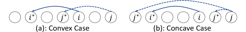
Figure 1. Convex and concave decision monotonicity. (a). Convexity: for two states $i<j$, their best decisions satisfy $i^{*}\leq j^{*}$. (b). Concavity: for two states $i<j$, their best decisions satisfy either $j^{*}\leq i^{*}$ or $j^{*}\geq i$.

Related Work.   Dynamic programming (DP) is one of the most studied topics in algorithm design. The seminal survey by Galil and Park (1992) reviewed two types of optimization techniques sequentially, including decision monotonicity (e.g., (Klawe, 1989; Klawe and Kleitman, 1990; Wilber, 1988; Eppstein et al., 1992b; Galil and Park, 1992; Eppstein, 1990; Galil and Park, 1989; Klawe, 1989)) and sparsity (e.g., (Eppstein et al., 1990, 1992a; Hirschberg, 1977; Hunt and Szymanski, 1977)). In this paper, we mainly focus on parallelizing the sequential algorithms in this scope, and we will review the literature of each problem in the corresponding section.

DP is also widely studied in parallel. There exists rich literature on optimizing various goals in different models, such as span (time) in PRAM (e.g. (Galil and Park, 1994; Apostolico et al., 1990; Babu and Saxena, 1997; Lu and Lin, 1994; Larmore and Rytter, 1994; Atallah et al., 1989; Huang et al., 1994; Larmore and Przytycka, 1995; Rytter, 1988; Larmore and Przytycka, 1996; Larmore et al., 1993)), I/O cost in the external-memory/ideal-cache model (e.g., (Chowdhury and Ramachandran, 2006, 2008, 2010; Chowdhury et al., 2016; Itzhaky et al., 2016; Tang et al., 2015)), rounds in the MPC model (Im et al., 2017; Boroujeni and Seddighin, 2019; Gupta et al., 2023; Bateni et al., 2018), or on the BSP model (Krusche and Tiskin, 2009, 2010; Alves et al., 2002). However, these papers either only considered the DP algorithms without the optimizations, or incur polynomial work overhead, except for (Chan and Lam, 1990; Bradford et al., 1998) for one specific problem. Instead, our paper tries to parallelize the efficient and practical sequential algorithms while maintaining low work. Some other works try to parallelize certain types of DP or applications using DP (e.g., (Awan et al., 2020; Aimone et al., 2019; Blelloch et al., 2016b; Weiss and Schwartz, 2019; Javanmard et al., 2019; Li et al., 2014)). Alternately, our work aims to provide a general approach to parallelize almost all DP algorithms.

2   Model and Framework

We use the work-span model in the classic multithreaded model with binary-forking (Arora et al., 2001; Blelloch et al., 2020b; Blumofe and Leiserson, 1999). We assume a set of threads that share the memory. Each thread acts like a sequential RAM plus a fork instruction that forks two threads running in parallel. When both threads finish, the original thread continues. A parallel-for is simulated by forks in a logarithmic number of steps. A computation can be viewed as a DAG. The work $W$ of a parallel algorithm is the total number of operations, and the span (depth) $S$ is the longest path in the DAG. In practice, we can execute the computation with work $W$ and span $S$ using a randomized work-stealing scheduler (Blumofe and Leiserson, 1999; Gu et al., 2022) in time $W/P+O(S)$ with $P$ processors with high probability. A parallel algorithm is work-efficient, if its work is $O(W)$, where $W$ is the work of the best known or the corresponding sequential algorithm, and nearly work-efficient if its work is $\tilde{O}(W)$. We use $\tilde{O}(\cdot)$ to hide ${\mbox{{polylog}}}(n)$ where $n$ is the input size.

2.1   Basic Concepts in Dynamic Programming

A DP algorithm solves an optimization problem by breaking it down to subproblems, memoizing the answers to the subproblems, and using them to find the answer to the original problem. The subproblems are usually indexed by integers, referred to as states. With clear context, we directly use $i$ to refer to “state $i$”. The DP value of a state is determined either by a boundary condition (i.e., initial values), or from other states, specified by a DP recurrence. This paper studies recurrences in the following form:

(1) $$D[i]={\min/\max}~{}f_{i,j}(D[j])$$

where $j$ is a decision at $i$. Function $f_{i,j}(\cdot)$ indicates how the DP value of state $j$ can be used to update state $i$. The transitions (i.e., dependencies) among states form a DAG $G=(V,E)$ as introduced in Sec. 1. We use $j\rightarrow i$ to denote an edge from $j$ to $i$ in the DAG.

During a DP algorithm, we may maintain the DP value of a state and update it by the recurrence. We call the process of updating $D[i]$ by $D[j]$ a relaxation, or say $j$ relaxes $i$. A relaxation is successful if the DP value is updated to a better value, i.e., a lower (higher) value if the objective is minimum (maximum). We call the actual DP value of a state the true or finalized DP value to distinguish from the DP value being updated during the algorithm, which we call the tentative DP value. We say a state $i$ is finalized if we can ensure that its true DP value has been computed, and tentative otherwise. Among all tentative states, we say a state is ready, if all its decisions are finalized, and unready otherwise. A naïve DP algorithm will process all transitions and states based on a topological ordering.

DP Optimizations.   Instead of computing the recurrence straightforwardly, many algorithms can optimize the computation by skipping vertices and/or edges in the DAG to save work. We call such algorithms optimized DP algorithms. For example, given an input sequence $A[1..n]$, the optimized LIS algorithm (Knuth, 1973) maintains a data structure to precisely find the best decision of each state in $O(\log n)$ cost, and only processes $O(n)$ transitions instead of $O(n^{2})$ as suggested by the recurrence. Similarly, given two input sequences $A[1..n]$ and $B[1..m]$, the optimized LCS algorithm only needs to process all states $D[i,j]$ where $A[i]=B[j]$, instead of $O(nm)$ states in the recurrence. Another typical optimization is decision monotonicity where the best decisions of previous states can narrow down the range for best decisions for later states, which skips transitions and saves work. Typical examples include concave/convex generalized LWS (see Sec. 4), OAT (see Sec. 5.1), GAP (see Sec. 5.2), etc. We will discuss all these algorithms in this paper.

2.2   Parallelizing Sequential DP Algorithms

We now discuss our goal to parallelize a sequential DP algorithm. Our primary goal is to achieve (asymptotically) the same computation as an optimized sequential algorithm. More formally, for a sequential algorithm $\Gamma$ computing a recurrence $R$ with certain optimizations, we define the $\Gamma$-optimized DAG, denoted as $G_{\Gamma}=(V_{\Gamma},E_{\Gamma})$, as follows. $G_{\Gamma}$ is the same as the DP DAG on $R$ with some edges highlighted: for all edges that are processed by $\Gamma$, we highlight them in $G_{\Gamma}$, and call them the effective edges. We call the other edges normal edges. These effective edges can be used to fully complete the computation. For a sequential DP algorithm $\Gamma$, we hope its faithful and best possible parallelization $\Lambda$ to:

• process the same effective edges in $G_{\Gamma}$ and achieve the same work as $\Gamma$, and

• have span proportional to the effective depth of $G_{\Gamma}$, defined as the largest number of effective edges in any path in $G_{\Gamma}$.

Namely, if our goal is to parallelize $\Gamma$ and perform the same computation, the parallel algorithm $\Lambda$ has to process all edges $j\rightarrow i$ processed by $\Gamma$. This means $i$ can be finalized only after j is finalized, so the span is related to the effective depth as defined above. We use $\hat{E}_{\Gamma}$ to denote the set of effective edges, and $\hat{d}(G_{\Gamma})$ as the effective depth of $G_{\Gamma}$. More formally, we define the following concepts.

We say a parallel algorithm $\Lambda$ is an optimal parallelization of a sequential DP algorithm $\Gamma$, if 1) the set of edges processed in $\Lambda$ and $\Gamma$ satisfies $\hat{E}_{\Gamma}\subseteq\hat{E}_{\Lambda}$ and $|\hat{E}_{\Lambda}|=O(|\hat{E}_{\Gamma}|)$, 2) the work of the two algorithms are asymptotically the same, and 3) the span of $\Lambda$ is $\tilde{O}(\hat{d}(G_{\Gamma}))$. Namely, $\Lambda$ can process a superset of edges of that in $\Gamma$, but not asymptotically more, and its span is proportional to the effective depth of the $\Gamma$-optimized DAG.

In addition, we define the perfect parallelization. In an omniscient version of $\Gamma$, we only need to process the best decisions based on their dependencies. We define the $\Gamma$-perfect DAG, denoted as $G^{*}_{\Gamma}$, as subgraph of $G_{\Gamma}$ that only contains the best decision edges (both effective and normal edges). We say an optimal parallelization $\Lambda$ of $\Gamma$ is also a perfect parallelization if the span of $\Lambda$ is $\tilde{O}(\hat{d}(G^{*}_{\Gamma}))$.

While the definitions seem abstract, we will later show that they are intuitive for concrete problems. For example, in longest common subsequence (LCS), both $\hat{d}(G_{\Gamma})$ and $\hat{d}(G^{*}_{\Gamma})$ are the output LCS length $k$ (but for other algorithms they can be different), and our goal is to achieve $\tilde{O}(k)$ span for a perfect parallelization.

Note that the “perfect parallelization” of a sequential algorithm does not directly suggest optimality in work or span bounds for the same problem. One can possibly achieve better bounds by redesigning the recurrence and/or sequential algorithm with fewer edges or a shallower depth. Instead of finding or redesigning a different DAG to obtain new optimizations, our focus is to provide parallelization of existing sequential algorithms with optimizations.

In the following, we first present our new algorithmic framework: the Cordon Algorithm, which provides a correct, although not necessarily efficient parallelization for general DP algorithms. On top of it, for each specific problem, we will show how to achieve low work, which, as discussed in Sec. 4 and 5, can be highly non-trivial.

2.3   Our Framework: the Cordon Algorithm

Our idea is based on the phase-parallel framework (Shen et al., 2022) (see below) adapted to DP algorithms. The phase-parallel framework by Shen et al. aims to identify (as many as possible) operations that do not depend on each other, and process them in parallel. Directly applying this framework to DP algorithms will give the following algorithm outline:

While there exist any tentative states: • Find the set of ready states as $\mathcal{F}$ • Process all states in $\mathcal{F}$ in parallel and mark all of them as finalized

We call each iteration of the while-loop a round. We call the set of states being processed in round $i$ the frontier of round $i$, noted as $\mathcal{F}_{i}$. While the phase-parallel framework gives a high-level approach in achieving parallelism, it does not indicate how to do so (i.e., how to identify the ready states in each round).

We now introduce our Cordon Algorithm, which uses a novel approach to identify the frontier $\mathcal{F}_{i}$ in each round, particularly for a DP computation $G_{\Gamma}$. The Cordon Algorithm identifies the unready tentative states and put sentinels on them; then it uses all sentinels to outline a cordon to mark the boundary of the frontier. We summarize the algorithm in the following steps. Note that every step can be processed in parallel.

1. Mark all states as tentative and initialize them by the boundary condition.

2. If a tentative state $j$ can successfully relax another tentative state $i$ (i.e., update $D[i]$ to a better value), put a sentinel on state $i$. Such a sentinel means that all the descendants (inclusive) of state $i$ are unready. We say this state and all its descendants are blocked by the sentinel in this case. Therefore, a state is ready if there is no sentinel on any of its ancestors (inclusive).

3. For each ready state, use its DP value to relax the tentative DP values of its descendants. Usually, we need to do so implicitly to achieve efficient work. We discuss more details later.

4. Mark all ready states as finalized. Clear all the sentinels.

5. If there still exist tentative states, go to Step 2 and repeat.

We will first prove that the algorithm is correct, i.e., it computes correct DP values for all states. Later we will show some motivating examples to help understand this algorithm in Sec. 3.

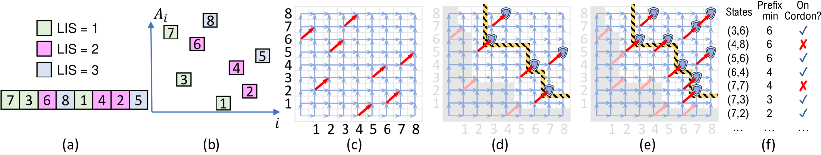
Figure 2. Illustrations for the LIS/LCS problem and the Cordon Algorithm. Subfigure (a): An input sequence for LIS with the DP value of each element. Subfigure (b): A geometric view of the input sequence on a 2D plane with each element represented as $(i,A_{i})$. Subfigure (c): The corresponding LCS on this input—the answer is the longest path from $(0,0)$ to $(8,8)$ using the maximum number of red edges. Subfigure (d): The process to compute the second cordon. The ready states are marked in the shaded gray region. The cordon is decided by the three cells with LIS=2 in the original input. Subfigure (e): A general LCS case where every diagonal can be a red edge. Subfigure (f): An example execution of our LCS algorithm. Here we only show unready states for simplicity.

Theorem 2.1.

The Cordon Algorithm is correct.

• This is equivalent to show that, when we find a ready state and later mark it finalized, its DP value must be finalized.

  We will show this inductively. At the beginning, the ready states are those with zero in-degree in the DAG, and their true DP values are specified by the boundary cases. Clearly, their DP values cannot be relaxed by other states and they will be identified as ready in our algorithm. Their DP values are also computed by the boundary in Step 1. Therefore, our algorithm is correct in the first round.

  Assume the algorithm is correct up to round $r$. We will show that round $r+1$ also correctly finds the ready states and their DP values. Assume to the contrary that a state $i$ identified in Step 2 does not have its true DP value yet. This means that the best decision of $i$ has not relaxed $i$ to the finalized value. Let $j=\mathit{best}[i]$. Note that $j$ cannot be finalized: if so, before $j$ is marked as finalized in Step 4, in Step 3 it must have relaxed $i$.

  Therefore, $j$ is tentative. In this case, let $j_{0}=i$, and state $j_{x}$ be the best decision of state $j_{x-1}$ for $x\geq 1$, i.e., we chase the chain of best decisions and get a list of states $i=j_{0},j_{1}=\mathit{best}[j_{0}]$, etc. Let us find the first $x$ such that $D[j_{x}]$ is not the true DP value but $D[j_{x+1}]$ is the true DP value. We then prove that state $j_{x+1}$ must be a tentative state. If we consider $j_{y}$ as the first finalized state on this chain, then $j_{y-1}$ is a tentative state, and also must already have its true DP value (because $j_{y}$ has relaxed it in Step 3). Note that since state $j_{y-1}$ is a tentative state, all states between $j_{0}$ and $j_{y-1}$ must be tentative. Since $j_{y-1}$ has its true DP value, and $i=j_{0}$ does not have its true DP value, the first switch point $j_{x}$ must be between $j_{0}$ and $j_{y-1}$, and must also be a tentative state.

  Therefore, state $j_{x+1}$ is a tentative state that can relax state $j_{x}$, so it will put a sentinel on state $j_{x}$. As a descendant of $j_{x}$, state $i$ must be blocked by $j_{x}$, and cannot be identified as a ready state. This leads to a contradiction. Therefore, if a state $i$ is identified as ready in our algorithm, its DP value must have been finalized. ∎

The Cordon Algorithm tells which states/vertices should be in the frontier in each round, but the algorithm does not show how to do so efficiently. Especially in Step 3, it is almost infeasible to use the finalized DP values to explicitly update all other states. In this case, we have to develop new parallel data structures to facilitate this step. Next, we first use LIS and LCS as two examples to illustrate our framework. We then apply it to more involved cases that use decision monotonicity in Sec. 4 and 5.

3   Motivating Examples on LIS/LCS

To help the audience understand the more complicated algorithms using DM in the following sections, we first provide two simple examples on Cordon Algorithm, especially on how to compute the cordon efficiently.

Longest Increasing Subsequence (LIS).   We first use LIS as an example. Given an input sequence $A_{i}$, LIS computes the maximum of $D[i]$ such that:

(2) $$D[i]=\max\{1,\max_{j<i,A_{j}<A_{i}}D[j]+1\}$$

We use $n$ as the input size and $k$ as the output LIS length. Directly computing this recurrence takes $O(n^{2})$ work. Sequentially, we can process all states one by one, and compute $\max_{j<i,A_{j}<A_{i}}D[j]$ using a binary search structure, giving $O(n\log k)$ total cost (Knuth, 1973). The binary search precisely finds the best decision of each state, and only $n$ transitions are processed. Many parallel LIS solutions have also been proposed (Shen et al., 2022; Gu et al., 2023; Cao et al., 2023; Krusche and Tiskin, 2009, 2010). We will show that solving LIS using our Cordon Algorithm framework will essentially give an existing algorithm (Gu et al., 2023) and is a perfect parallelization of the sequential $O(n\log k)$ algorithm.

Based on Cordon Algorithm, the boundary case is to set all tentative DP values as 1. Then we will attempt to use the current tentative DP values for relaxation. In this case, for a state $i$, as long as there is any other state $j<i$ with $A_{j}<A_{i}$, $D[i]$ can be relaxed to a better value 2. Therefore, all ready states are those input objects that are prefix-min elements in the sequence, i.e., $A_{i}$ is the smallest value among all $A_{1..i}$. We can set these states as ready, update all other states and repeat. Note that since all unfinalized states have the same tentative DP value of 2, we do not need to explicitly update the values in $D[i]$, but can just maintain a global variable as the current tentative DP value. By the same idea, the ready states in the next round would be the prefix-min elements in the input after removing the finalized states. The same observation (repeatedly finding prefix-min elements) is exactly the core idea of the algorithm in (Gu et al., 2023). In their algorithm, they further use a tournament tree to identify prefix-min elements efficiently and achieve efficient $O(n\log k)$ work, and $O(k\log n)$ span. Note that $k$ is exactly the perfect depth of the DP DAG, which is the longest dependency between best decisions.

Theorem 3.1.

Combining with a tournament tree, Cordon Algorithm leads to a perfect parallelization of sequential $O(n\log k)$ LIS algorithm in (Gu et al., 2023), where $n$ is the input size, and $k$ is the LIS length.

Longest Common Subsequence (LCS).   LIS has a close relationship with other important problems such as LCS. Here we will revisit our cordon-based LIS algorithm from the view of LCS, which also leads to a new parallel LCS algorithm. Given two sequences $A[1..n]$ and $B[1..m]$ ($m\leq n$), LCS aims to find a common subsequence $C$ of $A$ and $B$ such that $C$ has the longest length among all common subsequences. An LIS problem can be reduced to an LCS problem by first relabeling all input elements by $1..n$ based on their total order, and then finding the LCS between this new sequence and a sequence $B=\langle 1,2,\dots,n\rangle$. See Fig. 2(a)–(c) for an illustration. LCS has been extensively studied both sequentially (Hunt and Szymanski, 1977; Hirschberg, 1977; Apostolico and Guerra, 1987; Eppstein et al., 1992a; Knuth, 1973) and in parallel (Lu and Lin, 1994; Tchendji et al., 2020; Babu and Saxena, 1997; Xu et al., 2005; Apostolico et al., 1990; Chen et al., 2006; Ding et al., 2023). The standard DP solution defines each state $D[i,j]$ as the LCS for $A[1..i]$ and $B[1..j]$, and uses the following recurrence:

(3) $$\small D[i,j]=\begin{cases}0,&\mbox{if }i=0\mbox{ or }j=0\\ D[i-1,j-1]+1,&\mbox{if }A[i]=B[j]\\ \max\{D[i-1,j],D[i,j-1]\},&\mbox{otherwise}.\end{cases}$$

These transitions correspond to horizontal, vertical and diagonal edges on a grid (see an example in Fig. 2(c)). A known sequential optimization (i.e., sparsification) (Hunt and Szymanski, 1977; Hirschberg, 1977; Apostolico and Guerra, 1987; Eppstein et al., 1992a) to this recurrence is to observe that only the edges correspond to the diagonal edges with $A[i]=B[j]$ are useful. The computation is equivalent to finding the longest path from the bottom-left to top-right corresponds to these effective (red) edges, and all other edges and states can be skipped. This can lead to a sequential algorithm with $O(L{}\log n)$ cost, where $L{}$ is the number of pairs $(i,j)$ such that $A[i]=B[j]$. For LIS, there are exactly $L{}=n$ such effective edges.

We will show how Cordon Algorithm can be used to parallelize this optimization. Starting with the boundary where $D[i,j]=0$, we observe that the DP value $D[i,j]$ of any state with $A[i]=B[j]$ can be updated to a better value. Therefore, we will put a sentinel at each of such states to indicate that they should be updated. All such sentinels will block the top-right part of the grid. In this way, the blocked region is clearly marked by a staircase region, as shown in Fig. 2(d). Therefore, the entire region within the first cordon has the DP value 0. By repeatedly doing this, we will effectively find that the region between the cordons of round $i+1$ and $i$ are those states with DP value (LCS length) $i$. The algorithm finishes in $k$ rounds where $k$ is the LCS length.

The problem boils down to efficiently identifying the cordon (i.e., the staircase) in each round. Note that in LIS there is at most one effective edge in each column (see Fig. 2(d)), while in LCS there can be multiple effective edges in each column (see Fig. 2(e)). We will show an interesting modification to the original LIS algorithm that can handle this more complicated setting. Here we sort all edges by column index as the primary key (from the smallest to largest) and row index as the secondary key (but from largest to smallest). An example is illustrated in Fig. 2(f). Then, we will still use a tournament tree to maintain this list, and apply prefix-min on the row indexes. It is easy to see that a state/edge is on the cordon if its row index is smaller than or equal to the prefix-min. A tournament tree can identify, mark, and remove these states in $O(l\log(L/l))$ work and $O(\log n)$ span (Gu et al., 2023), where $l$ is the number of diagonal edges on the cordon. We thus have the following theorem.

Theorem 3.2.

Combining with a tournament tree, Cordon Algorithm leads to a perfect parallelization ($O(L{}\log n)$ work and $O(k\log n)$ span) of sequential LCS algorithm in (Apostolico and Guerra, 1987), where $n$ and $m<n$ are the input sequence sizes, $L$ is the number of pairs $(i,j)$ such that $A[i]=B[j]$, and $k$ is the LCS length.

Since $L=O(n^{2})$, the $O(\log L)$ terms in the cost of the tournament trees is stated as $O(\log n)$ in the theorem.

Interestingly, to the best of our knowledge, this is the first parallel LCS algorithm with $o(mn)$ work and $o(\min(n,m))$ span for sparse LCS problem (i.e., $L=o(mn)$ and $k=o(\min(n,m))$). Meanwhile, this algorithm is quite simple—we provide our implementation in (Ding et al., 2024) and experimentally study it in Sec. 6. Another interesting finding is that our algorithm implies how to map LCS to LIS (previously only the other direction is known). Given two input strings $A$ and $B$, if we sort all $(i,j)$ pairs for $A_{i}=B_{j}$ by increasing $i$ (primary key) and decreasing $j$ (secondary key), then LCS is equivalent to the LIS on the secondary keys (the $j$(s)) of this sorted list.

We will show more sophisticated parallelization of DP algorithms in the next sections. Our LCS algorithm will be a subroutine in the more involved parallel GAP algorithm introduced in Sec. 5.2.

4   Parallel Generalized LWS

We now discuss the convex/concave generalized least weight subsequence (GLWS) problem, which is one of the most classic cases of decision monotonicity (DM). Given a cost function $w(j,i)$ for integers $0\leq j<i\leq n$ and $D[0]$, the GLWS problem computes

(4) $$D[i]=\min_{0\leq j<i}\{E[j]+w(j,i)\}$$

for $1\leq i\leq n$, where $E[j]=f(D[j],j)$ can be computed in constant time. The original least weight subsequence (LWS) problem (Hirschberg and Larmore, 1987) is a special case when $E[j]=D[j]$. Here we use the general case $E[j]=f(D[j],j)$ that has the same sequential work bound (Eppstein, 1990; Galil and Park, 1989; Klawe, 1989; Galil and Park, 1992; Eppstein et al., 1988; Eppstein et al., 1992b), because the generalized version is needed in many applications (see examples in Sec. 5). The GLWS problem is also referred to as 1D/1D DP by Galil and Park (1992). The GLWS problem is highly relevant to other important problems (e.g., line breaking (Knuth and Plass, 1981), optimal alphabetic trees (Larmore et al., 1993), and a number of computational geometry problems (Aggarwal and Klawe, 1990)). The essence of GLWS is to cluster a list of 1D objects based on spatial proximity and minimize the total weighted sum of all clusters. As an intuitive example, consider selecting a subset of villages on a road (with their coordinates known) to build post offices to minimize the total cost, where $w(j,i)$ is the cost of using one post office to serve villages $j+1$ to $i$. This gives a GLWS problem with $D[i]$ as the lowest cost to serve the first $i$ villages and $E[i]=D[i]$. The DP recurrence enumerates all possible decisions $j$ such that the last post office serves the villages $j+1$ to $i$, and takes the minimum cost among all possible decisions $j$. Practical cost functions $w$ (e.g., a fixed cost plus a linear or quadratic cost to the service range or sum of distances from villages to the post office) are convex, which implies DM—for two states $i$ and $j>i$, their best decisions $i^{*}$ and $j^{*}$ satisfy $j^{*}\geq i^{*}$. Symmetrically we can show that for concave cost functions $w$, either $j^{*}\geq i$ or $j^{*}\leq i^{*}$ holds, although concave cost functions are less common in the real-world applications of GLWS.

Given its high relevance in practice, convex GLWS has been studied in parallel. Apostolico et al. (1990) showed an algorithm with $O(n^{2}\log n)$ work and $O(\log^{2}n)$ span. Later, Larmore and Przytycka (1995) showed an improved algorithm with $O(n^{1.5}\log n)$ work and $O(\sqrt{n}\log n)$ span. Despite the interesting algorithmic insights in these algorithms, the polynomial overhead in work limits their potential to outperform the classic sequential solutions with $\tilde{O}(n)$ work (Eppstein, 1990; Galil and Park, 1989; Klawe, 1989; Galil and Park, 1992; Eppstein et al., 1988; Eppstein et al., 1992b). For the concave case, some works (Chan and Lam, 1990; Bradford et al., 1998) achieve near work-efficiency and polylog span on the original LWS, but the ideas cannot be applied to generalized LWS.

In this section, we show how to use the Cordon Algorithm to parallelize a well-known sequential GLWS algorithm with ${O}(n\log n)$ work, which works for both convex and concave DM. Although efficiently applying Cordon Algorithm here requires many sophisticated algorithmic techniques, our parallel algorithm (Alg. 1) remains practical and it indeed outperforms the sequential algorithm in a wide parameter range (see Sec. 6 for details). It is also the key building block for many other algorithms shown later in Sec. 5.

We start with preliminaries and the classic sequential algorithm, then discuss how to use Cordon Algorithm to parallelize it. We will use the convex case when describing the algorithm since it is used more often in practice, and discuss the concave case in Sec. 4.3.

4.1   Preliminaries

Convexity, Concavity and Decision Monotonicity.   The convexity of the cost function $w$ is defined by the Monge condition (Monge, 1781). We say that $w$ satisfies the convex Monge condition (also known as quadrangle inequality (Yao, 1980)) if for all $a<b<c<d$,

(5) $$w(a,c)+w(b,d)\leq w(b,c)+w(a,d).$$

We say that $w$ satisfies the concave Monge condition (also known as inverse quadrangle inequality) if for all $a<b<c<d$,

(6) $$w(a,c)+w(b,d)\geq w(b,c)+w(a,d).$$

Consider two states $i$ and $j>i$ with best decisions $i^{*}$ and $j^{*}$. A convex weight function leads to DM such that $j^{*}\geq i^{*}$. A concave weight function leads to DM such that either $j^{*}\geq i$ or $j^{*}\leq i^{*}$.

Another condition closely related to the Monge condition is the total monotonicity (Aggarwal et al., 1987). We say a $n\times m$ matrix $A$ is convex totally monotone if for $a<b$ and $c<d$,

$$A(a,c)\geq A(a,d)\Rightarrow A(b,c)\geq A(b,d).$$

We say a $n\times m$ matrix $A$ is concave totally monotone if for $a<b$ and $c<d$,

$$A(a,c)\leq A(a,d)\Rightarrow A(b,c)\leq A(b,d).$$

Let $c_{i}$ be the column index such that $A[i,c_{i}]$ is the minimum value in row $i$. The convex total monotonicity of $A$ implies that $r_{1}\leq r_{2}\leq...\leq r_{n}$, while in the concave case $r_{1}\geq r_{2}\geq...\geq r_{n}$ (Galil and Park, 1992). Also, if $A$ is convex totally monotone, any submatrix $B$ of $A$ is also convex totally monotone. The convex/concave Monge condition is the sufficient but not necessary condition for convex/concave total monotonicity.

In GLWS, we call $f_{i,j}=E[j]+w(j,i)$ a transition from $j$ to $i$. The convex/concave decision monotonicity is equivalent to the convex/concave total monotonicity of $f_{i,j}$. Note that if $w$ satisfies the convex/concave Monge condition, so does $f_{i,j}$. But the convex/concave total monotonicity of $w$ does not guarantee the convex total monotonicity of $f_{i,j}$. Throughout this paper, we assume the convex/concave Monge condition of $w$, but all our theorems only need the convex/concave total monotonicity of $f_{i,j}$.

The Sequential Algorithm.   The best (sequential) work bound for convex GLWS is $O(n)$ (Larmore and Schieber, 1991; Klawe, 1989; Galil and Park, 1992), and $O(n\alpha(n))$ for the concave case (Klawe and Kleitman, 1990). However, both of them are mainly of theoretical interest since they are complicated and have large constants in both work and space usage. We parallelize a simpler and more practical algorithm with $O(n\log n)$ work (Galil and Park, 1992). This algorithm computes $D[1..n]$ in order. It implicitly maintains the best decision array $\mathit{best}[1..n]$. When the algorithm finishes computing $D[i]$, the algorithm updates $\mathit{best}[i+1..n]$ using $D[i]$, then $\mathit{best}[j]$ ($j>i$) will be the best decision of state $j$ among states $0$ to $i$.

However, maintaining and updating this array of size $n$ for $n$ iterations require quadratic work. Observe that after computing $D[i]$, $\mathit{best}[i+1..n]$ must be non-decreasing in the convex case, and must be non-increasing in the concave case (Galil and Park, 1992). Hence, the algorithm maintains a “compressed” version of $\mathit{best}[i+1..n]$ by a list of triples $([l,r],j)$, which indicates that all states between $l$ and $r$ have best decision $j$, i.e., $\forall i^{\prime}\in[l,r]$, $\mathit{best}[i^{\prime}]=j$. The list is maintained by a monotonic queue, which is a classic data structure based on double-ended queue, and is inherently sequential. In the $i$-th iteration, we can directly find the decision of state $i$ from the queue. After obtaining $D[i]$, the monotonic queue can be updated in $O(\log n)$ amortized cost to consider $i$ as the best decision for all later states. In total, this algorithm costs $O(n\log n)$ work. Here we refer to the audience to the original paper for details of this algorithm. We will call this algorithm $\Gamma_{\mathit{lws}}$. Making use of DM, $\Gamma_{\mathit{lws}}$ only processes transitions between each state $i$ and its best decision. The DAG $G_{\Gamma_{\mathit{lws}}}$ for this algorithm includes normal edges $j\rightarrow i$ for all $j<i$, and exactly $n$ effective edges $\mathit{best}[i]\rightarrow i$ for all states $i$.

Due to simplicity, this algorithm is usually the choice of implementation in practice. We will show a parallel version of this algorithm using Cordon Algorithm.

4.2   Parallel Convex GLWS

Input: problem size $n,D[0]$, cost function $w(\cdot,\cdot)$

Output: $D[1..n]$: the DP table

Maintains: $B$: an sorted array storing triples of $([l,r],j)$, meaning that for all $l\leq i\leq r$, the current best decision $\mathit{best}[i]=j$

1

2$\mathit{now}\leftarrow 0$

3 while $\mathit{now}<n$ do

4       $\mathit{cordon}\leftarrow$ FindCordon($\mathit{now}$)

5       ${\textsf{UpdateBest}}(\mathit{now},\mathit{cordon})$

6       $\mathit{now}\leftarrow\mathit{cordon}-1$

7return $D[1..n]$

8Function FindCordon($\mathit{now}$)

9       $\mathit{cordon}\leftarrow n+1$

10       for $t\leftarrow 1$ to $\log n$ do

11             $l\leftarrow\mathit{now}+2^{t-1}$

12             $r\leftarrow\min(n,\mathit{now}+2^{t}-1)$

13             ParallelForEach $j\in[l,r]$ do

14                   Let $\mathit{best}[j]$ be the current best decision of $j$ recorded by $B$

15                   $D[j]\leftarrow E[\mathit{best}[j]]+w(\mathit{best}[j],j)$ // relax $j$

16                   Binary search in $B$ and find $s_{j}=\min\{i:E[j]+w(j,i)<E[\mathit{best}[i]]+w(\mathit{best}[i],i)\}$, i.e., $i$ is the first state that can be successfully relaxed by $j$

17            $\mathit{cordon}\leftarrow\min(\mathit{cordon},\min_{l\leq j\leq r}s_{j})$

18             if $\mathit{cordon}\leq r+1$ then break

19            

20      return $\mathit{cordon}$

21Function UpdateBest($\mathit{now},\mathit{cordon}$)

22       Tree $T\leftarrow{\textsf{FindIntervals}}(\mathit{now}+1,\mathit{cordon}-1,\mathit{cordon},n)$

23       Flatten $T$ into array $B$

24       Merge adjancent intervals with the same best decision in $B$

25      

26Function FindIntervals($j_{l},j_{r},i_{l},i_{r}$) // use $D[j_{l}..j_{r}]$ to update $\mathit{best}[i_{l}..i_{r}]$

27       if $i_{l}>i_{r}$ then return null

28       if $j_{l}=j_{r}$ then  return a leaf node$([i_{l},i_{r}],j_{l})$

29      

30      $i_{m}\leftarrow(i_{l}+i_{r})/2$

31       $j_{m}\leftarrow\operatorname*{\arg\!\min}_{j_{l}\leq j\leq j_{r}}(E[j]+w(j,i_{m}))$

32       $x\leftarrow$ node$([i_{m},i_{m}],j_{m})$

33       In Parallel:  

34             $T_{l}\leftarrow$FindIntervals($j_{l},j_{m},i_{l},i_{m}-1$)

35             $T_{r}\leftarrow$FindIntervals($j_{m},j_{r},i_{m}+1,i_{r}$)

36      return node $x$ with left child as $T_{l}$ and right child as $T_{r}$

Algorithm 1 Parallel Convex GLWS

We first give the parallel algorithm of convex GLWS. We will use the “post-office” problem mentioned above as a running example to explain the concepts, but our algorithm works for general cases.

Following the idea of the phase-parallel algorithm, with the current finalized states, the goal is to find all ready states as the frontier, where their true DP values can be computed from the finalized ones. We will use our Cordon Algorithm to find the frontier in each round. Naïvely, the recurrence suggests that a state depends on all states before it. However, note that a state is essentially ready as long as its best decision has been finalized. For the convex case, we will use the fact as shown below.

Fact 4.1.

In convex GLWS, let $S=\{j:j>i\wedge\mathit{best}[j]\leq i\}$, which is the set of states with best decisions no later than state $i$; then $S$ is a consecutive range of states starting from $i+1$.

This is a known fact in the sequential setting (can be proved by induction). It suggests that the frontier of each round in the phase-parallel algorithm is a consecutive range of states. Based on this idea, we will maintain $\mathit{now}$ as the last finalized state in each round. Then in the next round, ideally, the algorithm should find the cordon at $\mathit{cordon}$, where all states $[\mathit{now}+1,\mathit{cordon}-1]$ are ready and can compute their true DP value from (i.e., have their best decisions at) states no later than $\mathit{now}$. We show an example of the post-office problem to illustrate the phase-parallel framework in Fig. 3. Based on the discussions above, ideally, in round $i$, the ready states in the frontier are those where the best solution contains $i$ post offices. This is because their best decision must have $i-1$ post offices, and must be finalized in the previous round.

This high-level idea is presented in the main function of Alg. 1. Starting from $\mathit{now}=0$, given the current finalized states $[0,\mathit{now}]$, we will find all ready states $[\mathit{now}+1,\mathit{cordon}-1]$ using the Cordon Algorithm, which essentially will find the cordon at $\mathit{cordon}$. We explain this part with more details in Sec. 4.2.1. Similar to the sequential algorithm, we also maintain a data structure $B$ to store all triples $([l,r],j)$ in order, which indicates that all states between $l$ and $r$ have best decisions at $j$. This data structure is essential to guarantee the efficiency of finding the next frontier, and also has to be updated after each round with the new DP values (Alg. 1).

4.2.1   Finding the Cordon

To find the ready states in each round, we use the Cordon Algorithm. Namely, with all states up to $\mathit{now}$ finalized, we can attempt to use the tentative states after $\mathit{now}$ to update other tentative DP values. Once we find any $j$ that can update $i$, we put a sentinel at $i$. Among all sentinels, the smallest (leftmost) one will give the final position of the cordon.

However, note that we cannot afford exhaustive checking for all pairs of states $(j,i)$. First of all, checking all possible $j>\mathit{now}$ may incur large overhead in work, since most of the later states are unready anyway. Ideally, the algorithm should check up to exactly the position of $\mathit{cordon}$ (but this would be a chicken-and-egg problem). To handle this, our idea is to use prefix-doubling (see function FindCordon in Alg. 1), which attempts to extend the cordon by a batch of $2^{t-1}$ states for increasing $t$ in each substep $t$. If the entire batch is ready—i.e., no states in $[\mathit{now}+1,\mathit{now}+2^{t})$ can be relaxed by each other, and all sentinels are outside the batch—we try a larger step and extend the cordon to $\mathit{now}+2^{t+1}$. During the process, we will maintain $\mathit{cordon}$ as the leftmost sentinel so far. Once we find $\mathit{cordon}$ is inside the batch, it means that this batch is not fully ready. Therefore, the process stops and returns the current value of $\mathit{cordon}$ to the main algorithm.

Using prefix doubling, the parallel algorithm may check more states than the ready ones, but the number of “wasted” states is at most twice of the “useful” ones which will be finalized in this round. Hence, the total number of processed states is $O(n)$.

We then discuss the way to avoid checking all states $i>j$ when $j$ puts sentinels. By DM, if $j$ can successfully relax $i$, then $j$ can also successfully relax all states $i..n$. Therefore, we only need to put a sentinel at the first such state $i$. Recall that we maintain all best decision triples in a data structure $B$ in sorted order. By DM, we can simply binary search ($O(\log n)$ cost) in $B$ to find $s_{j}$ as the first tentative state that can be updated by $j$, and put a sentinel there.

The FindCordon in Alg. 1 gives the full process as described above. Each iteration of the while-loop at Alg. 1 is a substep, which processes a batch of states in $[\mathit{now}+2^{t-1},\mathit{now}+2^{t})$ in substep $t$. Then for each state $j$ in this batch (in parallel), we use $B$ to find the first state that can be updated by $j$ and put a sentinel at this position $s_{j}$. Finally, the leftmost sentinel so far forms the cordon. When the cordon is within the current batch, the algorithm returns. We also show an illustration of this process in Fig. 3.

Lemma 4.0.

The function FindCordon has $O(h\log n)$ work and $O(\log^{2}n)$ span, where $h=\mathit{cordon}-\mathit{now}-1$ is the frontier size.

• As discussed above, the prefix doubling scheme may attempt to process up to $h^{\prime}$ states, where $h^{\prime}\leq 2h$. For each such state, we may binary search in $B$ to find $s_{j}$ in $O(\log n)$ cost, and check the condition on Alg. 1 in $O(1)$ cost. Therefore, FindCordon has work $O(h\log n)$ and span $O(\log^{2}n)$. ∎

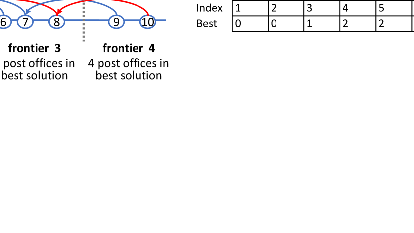
Figure 3. Example of applying the Cordon Algorithm to the post office problem with convex cost function. Circles (states) are villages. Arrows are best decisions between states. The final answer is four post offices serving villages 1–3, 4–7, 8–9, 10–12, respectively. The subrounds below illustrate the prefix-doubling scheme in FindCordon.

4.2.2   Generating New Best-Decision Array

The efficiency of the algorithm relies on maintaining an ordered data structure $B$ for all best decision triples. We will store $B$ as an array of all such triples in sorted order, such that the binary search in Alg. 1 can be performed efficiently. Therefore, after we get the newly finalized states $D[\mathit{now}+1..\mathit{cordon}-1]$, we need to update $B$ accordingly to get the new best decision for all states in $[\mathit{cordon},n]$.

We use a divide-and-conquer approach to do this. Function FindIntervals$(j_{l},j_{r},i_{l},i_{r})$ finds all best decision triples for states in range $[i_{l},i_{r}]$, with best decisions in range $[j_{l},j_{r}]$. Note that we only need the best decisions for all states after $\mathit{cordon}$. All these states must have their current best decisions within $[\mathit{now}+1,\mathit{cordon}-1]$ (if their best decisions are before $\mathit{now}$, they must have been ready in this round and been included in the frontier). Therefore, at the root level, we call FindIntervals$(\mathit{now}+1,\mathit{cordon}-1,\mathit{cordon},n)$.

In FindIntervals, we first compute $j_{m}=\mathit{best}[i_{m}]$ where $i_{m}=(i_{l}+i_{r})/2$, i.e., the best decision of the state in the middle. By (convex) DM, the best decisions of $i\in[i_{l},i_{m}-1]$ are in $[j_{l},j_{m}]$, and the best decisions of $i\in[i_{m}+1,i_{r}]$ are in $[j_{m},j_{r}]$. We will deal with the two subproblems in parallel. To collect all $([l,r],j)$ triples in parallel, we build a tree-based structure bottom-up in the recursion. Finally, we flatten the tree to an array and merge the adjacent intervals if they have the same value of $j$.

Lemma 4.0.

The function UpdateBest has $O(h\log n)$ work and $O(\log^{2}n)$ span, where $h=\mathit{cordon}-\mathit{now}-1$ is the frontier size.

• Flattening and removing duplicates can be performed by simple parallel primitives on trees and arrays in $O(h)$ work and $O(\log n)$ span. Below we will focus on the more complicated FindIntervals function. The span of FindIntervals comes from 1) $O(\log n)$ levels recursions and 2) $O(\log n)$ span to check all states in $[j_{l},j_{r}]$ in parallel. For the work, each recursive call in FindIntervals deals with a range of states $[i_{l},i_{r}]$ using best decision candidates in range $[j_{l},j_{r}]$. The algorithm first finds $i_{m}\in[i_{l},i_{r}]$ and its best decision $j_{m}\in[j_{l},j_{r}]$. This can be done by comparing all possible decisions in $[j_{l},j_{r}]$, which is $O(j_{r}-j_{l})$ work. split the ranges into two subproblems and recurse. Let $N=|i_{r}-i_{l}+1|$ and $M=|j_{r}-j_{l}+1|$ denoting the sizes of the two ranges. The work of FindIntervals indicates the following recurrence:

  $$W(N,M)=W(N/2,M_{1})+W(N/2,M_{2})+O(M),M_{1}+M_{2}=O(M)$$

  This solves to $O(M\log n)$. On the root level, $M=\mathit{cordon}-\mathit{now}-1=h$. This proves the stated work bound. ∎

4.3   Parallel Concave GLWS

To extend the algorithm to the concave case, we need a few modifications. In FindCordon, by the concavity, if $j$ can update $i$, then $j$ must be able to update $j+1$. Therefore, in Alg. 1 in Alg. 1, we check whether $j$ can update $j+1$. If so, we put a sentinel at $j+1$. The other modifications are in FindIntervals. First, due to concavity, when we find $j_{m}$ as the best decision of $i_{m}$ in Alg. 1, we need to swap the last two parameters in the first and second recursive calls, i.e., the best decision range for states $i_{m}+1$ to $i_{r}$ must be before $j_{m}$, and those in $i_{l}$ to $i_{m}-1$ must be after $j_{m}$.

A more involved modification in the concave GLWS is that after we get the array $B$ from FindIntervals, we have to merge it with the old array $B$ before this round—FindIntervals only considers the best decisions among $[\mathit{now}+1,\mathit{cordon}-1]$, but in the concave case, these states may also have better decisions using states before $\mathit{now}$. Suppose we have generated the array $B_{\mathit{new}}$ storing $([l,r],j)$ triples, and we want to merge it with $B_{\mathit{old}}$. Both of $B_{\mathit{old}}$ and $B_{\mathit{new}}$ contain the best decisions of states $[\mathit{cordon}..n]$. The difference is that the $j$s in $B_{\mathit{old}}$ are from $[0..\mathit{now}]$, while the $j$s in $B_{\mathit{new}}$ are from $[\mathit{now}+1..\mathit{cordon}-1]$. By the concave decision monotonicity, the key is to find a cutting point $p$, where the best decisions of $[\mathit{cordon}..p]$ are from $B_{\mathit{new}}$, and the best decisions of $[p+1,n]$ are from $B_{\mathit{old}}$.

1 ParallelForEach $([l_{k},r_{k}],j_{k})$ in $B_{\mathit{new}}$ do

2       $x_{k}\leftarrow$ search the best decision of $l_{k}$ from $B_{\mathit{old}}$.

3      

4Binary search the last $([l_{k},r_{k}],j_{k})$ in $B_{\mathit{new}}$ such that $E[j_{k}]+w(j_{k},l_{k})<E[x_{k}]+w(x_{k},l_{k})$.

5 Binary search the first $([l_{t},r_{t}],j_{t})$ in $B_{\mathit{old}}$ such that $E[j_{t}]+w(j_{t},r_{t})<E[j_{k}]+w(j_{k},r_{t})$.

6 Binary search the last $p$ in $[l_{k},r_{t}]$ such that $E[j_{k}]+w(j_{k},p)<E[j_{t}]+w(j_{t},p)$.

return $p$

Algorithm 2 Find the cutting point $p$

Here we show Alg. 2 to find $p$ in $O(h\log n)$ work and $O(\log n)$ span, where $h=|B_{\mathit{new}}|$ is the frontier size. For all $l_{k}$ in $B_{\mathit{new}}$, we pre-process its best decision stored in $B_{\mathit{old}}$. This step requires $O(h\log n)$ work and $O(\log n)$ span. Then we search in $B_{\mathit{new}}$ to find the interval that $p$ locates in. After this step, there is only one interval $([l_{k},r_{k}],j_{k})$ in $B_{\mathit{new}}$ is interesting. Then we can binary search in $B_{\mathit{old}}$ to find the exact $p$. Note that this method can be easily modified to merge $B_{\mathit{old}}$ and $B_{\mathit{new}}$ even if the cost function is convex.

4.4   Theoretical Analysis

In this section, we show theoretical analysis for our parallel GLWS algorithm. We first summarize our main results as follows.

Theorem 4.3.

Given an input sequence of size $n$, and the sequential GLWS algorithm $\Gamma_{\mathit{lws}}$ introduced in Sec. 4.1, let $k=\hat{d}(G^{*}_{\Gamma_{\mathit{lws}}})$ be the effective depth of the $\Gamma_{\mathit{lws}}$-perfect DAG. Then the Cordon Algorithm for the convex GLWS has $O(n\log n)$ work and $O(k\log^{2}n)$ span. It is a perfect parallelization of $\Gamma_{\mathit{lws}}$.

More intuitively, $k$ in Thm. 4.3 is also the number of best decisions to make in the final solution: for the post-office problem, it is the number of post offices in the optimal solution.

Theorem 4.4.

Given an input sequence of size $n$, and the sequential GLWS algorithm $\Gamma_{\mathit{lws}}$ introduced in Sec. 4.1, let $k=\hat{d}(G_{\Gamma_{\mathit{lws}}})$ be the effective depth of the $\Gamma_{\mathit{lws}}$-optimized DAG. Then the Cordon Algorithm for the concave GLWS has $O(n\log n)$ work and $O(k\log^{2}n)$ span. It is an optimal parallelization of $\Gamma_{\mathit{lws}}$.

We first prove that both algorithms are nearly work-efficient and have $O(n\log n)$ work.

Lemma 4.0.

The Cordon Algorithm for GLWS has $O(n\log n)$ work for both convex and concave case.

• Combining Lemma 4.1 and 4.2 (and the discussion in Sec. 4.3), the work for each round is $O(h\log n)$, where $h=\mathit{cordon}-\mathit{now}-1$ is the frontier size. Since the frontier sizes $h$ across all rounds add up to $n$, the entire algorithm has $O(n\log n)$ work. ∎

We then show that the number of rounds in both convex and concave cases is the effective depth of $G_{\Gamma_{\mathit{lws}}}$. Recall that the DAG $G_{\Gamma_{\mathit{lws}}}$ includes normal edges between all states $j$ and $i<j$, and effective edges between a state $j$ and its best decision. The effective depth $\hat{d}(G_{\Gamma_{\mathit{lws}}})$ is the largest number of effective edges in any path.

Lemma 4.0.

The Cordon Algorithm for GLWS finishes in $k$ rounds, where $k$ is $\hat{d}(G_{\Gamma_{\mathit{lws}}})$.

• Define the effective depth $\hat{d}(s)$ of a state $s$ as the largest number of effective edges of a path ending at $s$. We will inductively prove that a state $s$ is in the frontier of round $r$ iff. $s$ has effective depth $r$. The base case (boundary cases) holds trivially.

Assume the conclusion is true for $r-1$. We first prove the “if” direction, i.e., if a state $s$ has effective depth $r$, it must be in the frontier of round $r$. This is equivalent to show that there is no sentinel on all states from $\mathit{now}$ to $s$. Assume to the contrary that there is a state $y\in(\mathit{now},s]$ with a sentinel, which is put by state $x\in(\mathit{now},y]$. This means that $x$ is a better decision for $y$ than all states before $\mathit{now}$, indicating that $y$’s best decision $y^{*}\geq\mathit{now}$. Based on the induction hypothesis, the effective depth of $y^{*}$ must be larger than $r-1$. Therefore, $\hat{d}(y)=\hat{d}(y^{*})+1>r-1+1=r$, which means that $\hat{d}(y)$ is at least $r+1$. Based on the recurrence, there is a normal edge from $y$ to $s$, so $\hat{d}(s)\geq r+1$, leading to a contradiction.

We then prove the “only if” condition, i.e., if a state $s$ is in the frontier of round $r$, it must have effective depth $r$. The induction hypothesis suggests that all states with effective depth smaller than $r$ have been finalized in previous rounds, so we only need to show that $\hat{d}(s)$ cannot be larger than $r$. Assume to the contrary that $\hat{d}(s)\geq r+1$. Let the path to $s$ with effective depth $\hat{d}(s)$ be $x_{1},x_{2},\dots,s$. Since the total number of effective edges on this path is at least $r+1$, there must exist an effective edge $x_{i}\rightarrow x_{i+1}$ on the path such that $\hat{d}(x_{i})=r$ and $\hat{d}(x_{i+1})=r+1$. However, based on the induction hypothesis, $x_{i}$’s best decision must have been finalized. During Alg. 1, $x$ must get its true DP value, and will find itself able to update $x_{i+1}$. Therefore, there will be a sentinel on $x_{i+1}\leq s$, and $s$ cannot be identified in the frontier of round $r$. ∎

We will then show that the number of rounds of the convex case is also the effective depth of the $\Gamma_{\mathit{lws}}$-perfect DAG $G^{*}_{\Gamma_{\mathit{lws}}}$. This is stronger than the $\Gamma_{\mathit{lws}}$-optimized DAG as shown above. Recall that the perfect DAG $G^{*}_{\Gamma_{\mathit{lws}}}$ contains all best decision edges in $G_{\Gamma_{\mathit{lws}}}$.

Lemma 4.0.

The Cordon Algorithm for convex GLWS runs in $k^{*}$ rounds, where $k^{*}$ is $\hat{d}(G^{*}_{\Gamma_{\mathit{lws}}})$.

• Define the perfect depth $d^{*}(s)$ of a state $s$ as the largest number of effective edges of any path ending at $s$ in $G^{*}_{\Gamma_{\mathit{lws}}}$. Similarly, we will show by induction that in round $r$, all states with perfect depth $r$ will be processed. The base case holds trivially. Assume the conclusion holds for $r-1$. In round $r$, we will show that a state $s$ with perfect depth $r$ must be put in the frontier. Let $s^{*}$ be the best decision of $s$, then $d^{*}(s^{*})=r-1$ and therefore $s^{*}<\mathit{now}$. According to DM, any state $x$ between $\mathit{now}$ and $s$ must have its best decisions $x^{*}\leq s^{*}<\mathit{now}$, indicating that $d^{*}(x^{*})\leq r-1$. Therefore, $x$ must find its true best decision in $B$, and cannot be updated by any other tentative states in Alg. 1. This means that there will be no sentinel between $\mathit{now}$ and $s$, so $s$ must be identified ready in round $r$. Therefore, a state with perfect depth $r$ must be finalized in round $r$, leading to the stated theorem. ∎

Combining Lemma 4.1, 4.2, 4.6 and 4.7 proves the span bounds in Thm. 4.3 and 4.4.

5   Other Parallel DP Algorithms

We now show that our algorithmic framework can be used to parallelize a wide variety of classic sequential DP algorithms. In particular, for the optimal alphabetic tree (OAT) problem (Sec. 5.1), we partially answered a long-standing open problem by Larmore et al. (1993) for reasonable input instances (for instance, positive integer weights in range $n^{\operatorname*{polylog}(n)}$). For the GAP problem (Sec. 5.2), we showed the first nearly work-efficient algorithm with non-trivial parallelism. More interestingly, this algorithm combines all techniques in the algorithms for convex GLWS and sparse LCS.

5.1   Parallel Optimal Alphabetic Trees (OAT)

The optimal alphabetic tree (OAT) problem is a classic problem and has been widely studied both sequentially (Karpinski et al., 1997; Itai, 1976; Van Leeuwen, 1976; Nagaraj, 1997; Hu and Tucker, 1971; Garsia and Wachs, 1977; Davis, 1998; Larmore and Przytycka, 1998) and in parallel (Larmore and Przytycka, 1996; Rytter, 1988; Larmore et al., 1993; Larmore and Przytycka, 1995). Given a sequence of non-negative weights $a_{1..n}$, the OAT is a binary search tree with $n$ leaves and has the minimum cost, where the cost of a tree $T$ is defined as:

(7) $$cost(T)=\sum_{i=1}^{n}a_{i}d_{i}$$

Here $d_{i}$ is the depth of the $i$-th leaf (from the left) of $T$ (the root has depth 0). One can view the weight $a_{i}$ as the frequency of accessing leaf $i$, and the depth of a leaf is the cost of accessing it. Then the cost of $T$ is the total expected cost of accessing all leaves in $T$. The OAT problem is closely related to other important problems such as the optimal binary search tree (OBST) (Knuth, 1971) and Huffman tree (Huffman, 1952).

Sequentially, Hu and Tucker (1971) showed an OAT algorithm with $O(n\log n)$ work. Later Garsia and Wachs (1977) simplified this algorithm. In parallel, Larmore et al. (1993) showed an algorithm based on Garsia-Wachs. We will apply our techniques to this algorithm to improve the span bounds. Due to page limit, we provide the details of  (Larmore et al., 1993) in appendix A, and review the high-level idea here. The algorithm computes an $l$-tree (Garsia and Wachs, 1977), which has the same depth with and will be finally converted to the OAT in $O(n)$ work and polylogarithmic span. The key insight of  (Larmore et al., 1993) is to start with a sequence of $n$ leaf nodes with the input weights, and find several disjoint intervals in the sequence to process in parallel. This partition is done by various operations on the Cartesian tree of the input sequence, which requires $O(n\log n)$ work and $O(\log^{2}n)$ span. Larmore et al. showed that processing each interval can be reduced to a convex LWS. The solution of the LWS will connect items in this interval into a forest, which becomes a subgraph in the final $l$-tree. Finally, for each tree in the forest, we insert its root back to the sequence and repeat the process. This reinsertion step takes $O(n\log n)$ work and $O(\log n)$ span by basic parallel primitives such as sorting and range-minimum queries. The further rounds will connect the forest to the final $l$-tree. Larmore et al. also showed that the number of such intervals shrinks to half in each iteration, so the algorithm will finish in $O(\log n)$ rounds. Here all other steps in addition to solving convex LWS take $O(n\log^{2}n)$ work and $O(\log^{3}n)$ span. The remaining cost of the algorithm is to solve convex LWS in each round, multiplied by the number of rounds, which is $O(\log n)$.

Larmore et al. originally used the parallel convex LWS algorithm from (Apostolico et al., 1990; Alok and James, [n.d.]), which has $O(m^{2}\log m)$ work and $O(\log^{2}m)$ span when taking an input interval of length $m$. Later, Larmore and Przytycka (1995) improved the parallel convex LWS algorithm to $O(m^{1.5}\log m)$ work and $O(\sqrt{m}\log m)$ span, yielding $O(n^{1.5}\log^{2}n)$ work and $O(\sqrt{n}\log^{2}n)$ span for the OAT algorithm—the work overhead is still polynomial. Larmore et al. (1993) left the open problem on whether there exists an OAT algorithm with $\tilde{O}(n)$ work and $\operatorname*{polylog}(n)$ span, which remains unsolved for three decades.

Note that the convex LWS problem is a special case of the convex GLWS problem discussed in Sec. 4.1 with $E[i]=D[i]$. Hence, Alg. 1 directly gives $O(m\log m)$ work and $O(k\log^{2}m)$ span for convex LWS problem, and here $k$ is the longest dependency path of best decisions. In Larmore’s algorithm, the forest for each interval is constructed iteratively by the DP algorithm on LWS: if iteration $i$ finds the best decision at iteration $j<i$, then iteration $i$ creates one more level on top of the forest at iteration $j$. This means that the $k$ is equivalent to the depth of the forest, which is upper bounded by the final OAT height $h$. We present more details in appendix A. Hence, we can parameterize our final bounds using $h$ as:

Theorem 5.1.

The optimal alphabetic tree (OAT) can be constructed in $O(n\log^{2}n)$ work and $O(h\log^{3}n)$ span, where $n$ is the size of input weight sequence and $h$ is the height of the OAT.

This algorithm is nearly work-efficient with span parameterized on $h$. One useful observation is that the OAT height $h$ is polylogarithmic with real-world input instance with positive integer weights and fixed word length. More formally, we can show that:

Lemma 5.0.

If all input weights are positive integers in word size $W$, the OAT height is $O(\log W)$.

The proof is not complicated and we provide it in appendix A. With this lemma, we can state the following corollary.

Corollary 5.3.0.

If the input key weights are positive integers with word size $W=n^{\operatorname*{polylog}n}$, the OAT can be constructed in $O(n\log^{2}n)$ work and $\operatorname*{polylog}(n)$ span, where $n$ is the input size.

The bounds also hold for real number weights if the ratio between the largest and smallest weight is $n^{\operatorname*{polylog}n}$. We note that in realistic models we usually assume word-size $W=n^{O(1)}$, in which case Cor. 5.3 affirmatively answers the open problem in (Larmore et al., 1993).

5.2   The GAP Edit Distance Problem

The GAP problem is a variant of the famous edit distance problem. The GAP problem aligns two input strings with sizes $n$ and $m\leq n$, and allows editing a substring with certain cost function (see formal definition below). This problem has been widely studied both sequentially (Galil and Giancarlo, 1989; Eppstein et al., 1988; Chowdhury and Ramachandran, 2006) and in parallel (Blelloch and Gu, 2020; Chowdhury and Ramachandran, 2010; Galil and Park, 1994; Tang and Wang, 2017; Chowdhury et al., 2016; Itzhaky et al., 2016; Tithi et al., 2015). As noted by Eppstein et al. (1988), most real-world cost functions are either convex or concave, yielding $\tilde{O}(nm)$ work for the GAP problem sequentially. Unfortunately, to the best of our knowledge, these existing parallel algorithms for the GAP problem need $\Omega(n^{2}m)$ work, and the polynomial overhead makes them less practical.

More specifically, GAP takes two strings $A[1..n]$ and $B[1..m]$, and computes the minimum cost to align $A$ and $B$ using the following operations: 1) deleting $A[l+1..r]$ with cost $w_{1}(l,r)$, and 2) deleting $B[l+1..r]$ with cost $w_{2}(l,r)$. Here we consider the following recurrence, which is usually referred to as the GAP recurrence:

$$P[i,j] =\min_{0\leq i^{\prime}<i}D[i^{\prime},j]+w_{1}(i^{\prime},i)$$

$$Q[i,j] =\min_{0\leq j^{\prime}<j}D[i,j^{\prime}]+w_{2}(j^{\prime},j)$$

$$D[i,j] =\min\{P[i,j],Q[i,j],~{}D[i-1,j-1]~{}|~{}A[i]=B[j]\}.$$

Here $P[i,j]$ and $Q[i,j]$ indicate the edits on the two strings. Directly computing the recurrence uses $O(n^{2}m)$ work. Since most real-world cost functions in machine learning, NLP, and bioinfomatics (Eppstein et al., 1988) are either convex or concave, sequentially each row in $P$ or column in $Q$ is a convex or concave GLWS and can be computed in $\tilde{O}(n)$ or $\tilde{O}(m)$ work. Hence, computing the entire $P$ and $Q$ takes $\tilde{O}(nm)$ work, leading to the same cost for computing $D$ and the entire problem. We denote this standard sequential algorithm as $\Gamma_{\mathit{gap}}$.

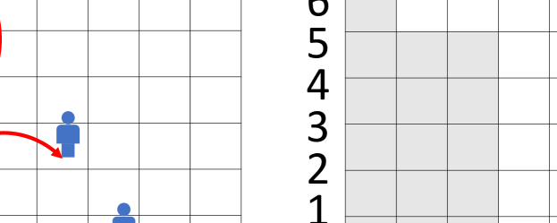
Figure 4. Example of a cordon in the GAP problem.

Parallelizing this approach is extremely challenging even with the parallel convex/concave GLWS in Sec. 4 as a subroutine, and we are unaware of any existing work on this. The challenge here is that the rows in $P$ interact with the columns in $Q$. For instance, computing a row in $P$ requires one element from each column in $Q$, but computing those elements again requires previous rows in $P$.

Our key insight to parallelize this algorithm is to use the Cordon Algorithm to efficiently mark the ready region to be computed in each round. Note that as a generalization of the classic edit distance/LCS, the GAP recurrence is similar to Recurrence 3, but with “jumps” in computing $P$ and $Q$. An illustration is given in Fig. 4. In addition to the diagonal edges as in LCS (see Fig. 2), for rows and columns, there also exist effective (red) edges (see Fig. 4(a)). Here for simplicity we only draw a subset of these edges, and every state $D[i,j]$ always have one vertical effective edge (to compute $Q[i,j]$), one horizontal effective edge (to compute $P[i,j]$), and may have a diagonal edge if $A[i]=B[j]$. All these edges imply the sentinels, which form the cordon and imply the regions for ready states, as shown in Fig. 4(b). The cordon is still a staircase as in LCS.

However, finding the cordon in GAP is sophisticated. We cannot directly use a tournament tree as in LIS, since the vertical and horizontal edges are computed on-the-fly and not known ahead of time. Meanwhile, in a 2D table where the cordon is a staircase, we cannot simply use prefix-doubling as in GLWS in Sec. 4. We propose a unique solution here to use prefix-doubling on a 2D table and computes the staircase cordon efficiently. This approach will consider each row separately, but for all rows, we run prefix doubling synchronously and try to see if the next ranges are available. First, we put a sentinel on state $(x,y)$ with a diagonal edge if $(x-1,y-1)$ is not finalized. We will maintain the best-decision structure for each row and column, in the same way as the GLWS algorithm. For this region to be checked, we will use the same approach as in Alg. 1 to compute $P$ and $Q$, take the minimum as $D$, and use $D$ to check their readiness. If a state $(x,y)$ obtains the best decision from another tentative state, we will put a sentinel on $(x,y)$, which will block the other states $(x^{\prime},y^{\prime})$ with $x^{\prime}\geq x$ and $y^{\prime}\geq y$. The work to put the sentinels is proportional to the number of states we checked in the prefix-doubling, and the span is polylogarithmic.

Finally we discuss how to handle the sentinels placed as above. We store all sentinels based on the row index on increasing order. After this, applying a prefix-min on these sentinels gives part of the cordon (if they exist), and we will merge it with the previous cordon. Then, for all tentative states, we check whether they are on the correct side, and invalidate those across the cordon. Since we are using prefix doubling, the wasted work for the invalid states can be amortized. In the next prefix doubling step, we will also use the cordon to limit the search region. Once all states within the cordon are checked for readiness, we can move to the next round. Due to prefix doubling, we only need $O(\log n)$ steps in each round.

Theorem 5.4.

The Cordon Algorithm for the GAP problem has $O(mn\log n)$ work and $O(k\log^{2}n)$ span, where $n$ and $m\leq n$ are the input size and $k$ is the effective depth of the $\Gamma_{\mathit{gap}}$-optimized DAG for the sequential algorithm $\Gamma_{\mathit{gap}}$ introduced in Sec. 5.2.

Proof of Thm. 5.4.   Recall that the sequential GAP algorithm $\Gamma_{\mathit{gap}}$ gets the DP value for each state $s=(i,j)$ by solving the GLWS problems in row $i$ and column $j$, respectively, and the diagonal edge $(i-1,j-1)\rightarrow(i,j)$ if applicable. Therefore, the optimal DAG $G_{\Gamma_{\mathit{gap}}}$ contains three types of edges

• $(i,j)\rightarrow(i^{\prime},j)$ for all $i^{\prime}>i$,

• $(i,j)\rightarrow(i,j^{\prime})$ for all $j^{\prime}>j$, and

• $(i-1,j-1)\rightarrow(i,j)$ if $A[i]=B[j]$.

Among them, the effective edges include:

• $(i,j)\rightarrow(i^{\prime},j)$ where $i$ is the best decision for $i^{\prime}$ in the GLWS problem on row $j$,

• $(i,j)\rightarrow(i,j^{\prime})$ where $j$ is the best decision for $j^{\prime}$ in the GLWS problem on column $i$, and

• $(i-1,j-1)\rightarrow(i,j)$ if $A[i]=B[j]$.

WLOG we assume $m\leq n$ in this section. We first prove the span bound. We will show that the Cordon Algorithm finishes in $k$ rounds, where $k$ is the effective depth of $G_{\Gamma_{\mathit{gap}}}$.

Lemma 5.0.

Given two sequences of sizes $n$ and $m\leq n$, the Cordon Algorithm on GAP edit distance finishes in $k=\hat{d}(G_{\Gamma_{\mathit{gap}}})$ rounds.

• The proof is similar to Lemma 4.6. We also define the effective depth of a state $s$ as $\hat{d}{s}$. We will show by induction that $s$ is processed in round $r$ iff. $\hat{d}{s}=r$. The base case holds trivially.

  Assume the conclusion holds for all rounds up to $r-1$. We will show it is also true for round $r$. We first prove the “if” direction, i.e., if a state $s=(i,j)$ ($i$-th row, $j$-th column) has effective depth $r$, it must be in the frontier of round $r$. This is equivalent to show that there is no sentinel that blocks $s$. For simple description, for two states $s=(i,j)$ and $s^{\prime}=(i^{\prime},j^{\prime})$, we say $s\prec s^{\prime}$ if $i\leq i^{\prime}$ and $j\leq j^{\prime}$. Clearly, if a state $s\prec s^{\prime}$, a sentinel on $s$ will block $s^{\prime}$. Assume to the contrary that there is a state $y\prec s$ with a sentinel, which is put by another tentative state $x\prec y$. This means that the tentative state $x$ is a better decision than all finalized states, indicating that the best decision of $y$, denoted as $y^{*}$, must also be tentative. Based on the induction hypothesis, the effective depth of $y^{*}$ must be larger than $r-1$. Therefore, $\hat{d}(y)\geq\hat{d}(y^{*})+1>r-1+1=r$, which means that $\hat{d}(y)$ is at least $r+1$. Let $y=(i^{\prime},j^{\prime})$. $y$ and $s$ can be connected by either one normal edge (when they are in the same row or column) or two normal edges ($(i^{\prime},j^{\prime})\rightarrow(i,j^{\prime})$ and $(i,j^{\prime})\rightarrow(i,j)$). This means that the effective depth of $s$ is at least the same as $y$, which is $r+1$. This leads to a contradiction.

  We then prove the “only if” condition, i.e., if a state $s$ is in the frontier of round $r$, it must have effective depth $r$. The induction hypothesis suggests that all states with effective depth smaller than $r$ have been finalized in previous rounds, so we only need to show that $\hat{d}(s)$ cannot be larger than $r$. Assume to the contrary that $\hat{d}(s)\geq r+1$. Let the path to $s$ with effective depth $\hat{d}(s)$ be $x_{1},x_{2},\dots,s$. Since the total number of effective edges on this path is at least $r+1$, there must exist an effective edge $x_{i}\rightarrow x_{i+1}$ on the path such that $\hat{d}(x_{i})=r$ and $\hat{d}(x_{i+1})=r+1$. However, based on induction hypothesis, $x_{i}$’s best decision must have been finalized. In round $r$, $x$ must get its true DP value, and will find itself able to update $x_{i+1}$. Therefore, there will be a sentinel on $x_{i+1}\prec s$, and $s$ cannot be identified in the frontier of round $r$. ∎

Combining Lemma 4.1 and 4.2, the span in each round is $O(\log^{2}n)$. This proves the span bound in Thm. 5.4.

We then prove the work bound in Thm. 5.4.

Lemma 5.0.

Given two sequences of sizes $n$ and $m\leq n$, the Cordon Algorithm on GAP edit distance has work $O(mn\log n)$.

• As $G_{\Gamma_{\mathit{gap}}}$ is a grid graph, its depth is no more than $m+n$. By Lemma 5.5 the algorithm will finish in $k=O(n)$ rounds. In each round, we do prefix-doubling across all $m$ rows and try to push the frontier on each row. In each prefix-doubling step we do a prefix-min that costs $O(m)$ work, so the cost of prefix-doubling is $O(m\log n)$ in each round, and $O(mn\log n)$ in total. Suppose $h$ is the frontier size in one round. Due to prefix-doubling, the number of tentative states we visited is at most $2h$. Combining Lemma 4.1 and 4.2, in each row/column we can achieve work proportional to the number of tentative states. Thus the cost to put sentinels and maintain the best decision arrays is also $O(mn\log n)$. ∎

5.3   General LWS on Trees

The idea of decision monotonicity (DM) can be applied to various structures more than just 1D cases discussed in Sec. 4. The efficient parallelism on 2D grid structure is introduced in Sec. 5.2, and we now show the techniques to enable high parallelism on the tree structure. Here we refer to this problem as Tree-GLWS.

Let $T$ be a tree with $n+1$ nodes, and node $0$ is the root. We use $p(v)$ to denote the parent of node $v$ and $d_{v}$ be the distance from node $0$ to node $v$. Tree-GLWS takes the input tree $T$, a cost function $w$, and the boundary $D[0]$, and computes:

(8) $$D[v]=\min\{E[u]+w(d_{u},d_{v})\}$$

where $u$ is any ancestor of $v$, and $E[u]=f(D[u],u)$ that can be computed in constant time from $D[u]$ and $u$. The cost function $w$ is decided by the depths of $u$ and $v$. Note that here sibling nodes $v_{1}$ and $v_{2}$ will have the same DP value, but $E[v_{1}]$ and $E[v_{2}]$ can be different given that $v_{1}$ and $v_{2}$ are also part of the parameter in computing the function $f$. In this section we assume $w$ is convex, but our algorithm can adapt to the concave case with some modifications.

5.3.1   Building Blocks

We will first overview some basic building blocks, which are crucial subroutines used in our algorithm.

Persistent Data Structures.   A persistent data structure (Driscoll et al., 1989) keeps history versions when being modified. We can achieve persistence for binary search trees (BSTs) efficiently by path-copying (Blelloch et al., 2016a; Sun et al., 2018; Blelloch et al., 2022), where only the affected path related to the update is copied. Hence, the BST operations can achieve persistence with the same asymptotical work and span bounds as the mutable counterpart.

Heavy-Light Decomposition (HLD).   HLD (Sleator and Tarjan, 1983) is a technique to decompose a rooted tree into a set of disjoint chains. In HLD, each non-leaf node selects one heavy edge, the edge to the child that has the largest number of nodes in its subtree. Any non-heavy edge is a light edge. If we drop all light edges, the tree is decomposed into a set of top-down chains with heavy edges. As such, HLD guarantees that the path from the root to any node $v$ contains $O(\log n)$ distinct chains plus $O(\log n)$ light edges. If we use BSTs to maintain each heavy chain in HLD, we can answer path queries (e.g., query the minimum weighted node on a tree path) in $O(\log^{2}n)$ work.

Range Report Based on Tree Depth.   We now discuss a data structure that efficiently reports the set of nodes in a subtree of $T$ where the depths of the nodes are in a given range $l$ to $r$. First we build the Euler-tour (ET) sequence of $T$, so any subtree of $T$ will be a consecutive subsequence in the ET. We can map all nodes to a 2D plane each with coordinates $(f_{v},d_{v})$, where $f_{v}$ is the first index of $v$ in the ET, and the $d_{v}$ is the tree depth of $v$. Now the original query is a 2D range report on this 2D plan. A range tree (Sun and Blelloch, 2019) can be built in $O(n\log n)$ work and $O(\log^{2}n)$ span, and answer this query in $O(m+\log^{2}n)$ work and $O(\log^{2}n)$ span where $m$ is the output size.

5.3.2   Our Main Algorithm

Here if we consider any tree path, Recurrence (8) is exactly the same as for the 1D case in Sec. 4. Hence, we can use a similar approach as in Sec. 4 by maintaining the best-decision array of $([l,r],j)$ triples, meaning that for elements $v$ with depth $l\leq d_{v}\leq r$, $v$’s best decision is $j$. The challenge here is the branching nature of a tree—we need to handle path divergences at nodes with more than one child. The work can degenerate to $\tilde{O}(n^{2})$ if we copy the best-decision arrays at the divergences, since we can end up with $O(n)$ leaves. Sequentially, we can depth-first traverse the tree and compute the “current” best-decision array, and we only need to revert the array when backtracking. However, this approach is inherently sequential. To utilize the Cordon Algorithm on a tree structure, we need to resolve the following two challenges: 1) how to efficiently identify the ready nodes; and 2) how to efficiently maintain the best decision arrays for each node.

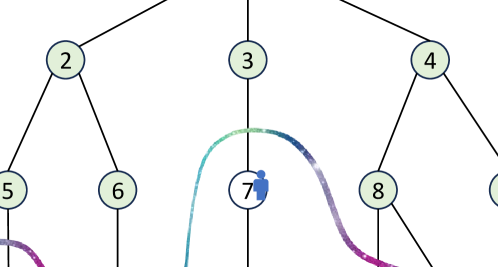
Figure 5. Cordon Algorithm on a tree. Note that the sibling nodes must have the same status.

Identifying the Ready States.   Similar to the 1D case Sec. 4, we maintain the best-decision array for each tree path. Then we traverse the tree top-down, and we identify the ready states $v$ that can be finalized in this round, and compute them in parallel. An illustration can be found in Fig. 5.

Our high-level idea still follows the prefix-doubling technique, similar to the 1D case. In the $t$-th doubling step we expand all nodes with $2^{t-1}\leq d_{v}<2^{t}$. These nodes can be extracted by a range report shown in Sec. 5.3.1. We use prefix doubling and the checking process in Sec. 4 to decide the boundary that forms the cordon in the next round. When checking the availability, we can use the HLD-based tree path query to find the minimum (highest) node on each path that is not available. We will put sentinels on these nodes that block their subtrees. The process stops when we find such nodes for all tree paths. In Fig. 5, these ready nodes are shown in green. In the next round we can asynchronously work on the subtrees on the cordon in parallel. We repeat this process until all nodes are finalized (correctly computed).

Here one difference to the 1D case is that the work cost of perfix doubling cannot be perfectly amortized. In the 1D GLWS, if the prefix-doubling stops at step $t$, we visit at least $2^{t-1}$ ready states and at most $2^{t-1}$ unready states, thus the work to visit the unready states can be amortized. However, in the tree case we are doing prefix-doubling by the depth of nodes. The number of nodes in the last prefix-doubling step can be much larger than in the previous steps, and the cost cannot be amortized. The insight is that due to the prefix-doubling, each node $v$ will be visited in at most $O(\log n)$ rounds. Plus the $O(\log^{2}n)$ work of the range report, the work in each round can be amortized to $O(h\log^{3}n)$, where $h$ is the frontier size.

Updating the Best-Decision Arrays.   The most interesting part in this algorithm is how to maintain the best-decision arrays for all tree paths while achieving work efficiency and high parallelism. Due to the tree structure, the best-decision arrays for different branches of the tree share some parts. In total, there can be $O(n)$ paths with total sizes of $O(n^{2})$. The key challenge is to save the work and space by sharing parts of the arrays, while updating them highly in parallel.

Consider the simple case when the ready nodes form a chain (the 1D case in Sec. 4). Here we use persistent BSTs to maintain the best-decision arrays on each node. We first use UpdateBestChoice in Alg. 1 to generate the best-decision array $B$ in the middle node of the chain, and merge it with the old $B$ (the one stored at the node above this chain) using the similar technique in Sec. 4.3. During this process we use path-copying to generate a new version the new array. Then we work on the upper part and the lower part of the chain in parallel. By this divide-and-conquer method, we can generate the best-decision array on each node of the chain with $O(m\log^{2}m)$ work and $O(\log^{3}m)$ span, where $m$ is the length of the chain.

In the general case, the structure of ready states can be arbitrary. To achieve work-efficiency and high parallelism, our solution is in a “BFS-style” algorithm that utilizes the properties of HLD (see Sec. 5.3.1). For all ready nodes in this round, we extend the heavy chain that is directly connected to the finalized nodes. Since the heavy chain will not diverge, the approach is the same as the 1D case except for additional persistence, with work proportional to the total number of nodes and polylogarithmic span. Once we finish updating the heavy chain, we will in parallel work on the light children of the nodes on the heavy chain we just proceeded. The overall structure is similar to a BFS with heavy edges with weight 0 and light edges with weight 1. Since each node only appears in one heavy chain, the work is still proportional to the number of ready nodes. We can also achieve high parallelism due to the fact that there can be at most $O(\log n)$ heavy chains and light edges from the root to any node $v$. Hence, we can finish updating all paths in a logarithmic number of steps per round, which guarantees both work-efficiency and high parallelism. Here we assume we build the HLD for the entire tree $T$ at the beginning, but we can also build the HLD for the ready states locally for each round.

Combining all pieces together, in each round we can determine the ready states and maintain the best-decision arrays with work proportional to the number of ready states and polylogarithmic span. We hence have the following theorem:

Theorem 5.7.

Cordon Algorithm solves Tree-GLWS in $O(n\log^{3}n)$ work and $O(k\log^{4}n)$ span, where $k$ is the longest path in the best decision dependency graph.

5.4   Parallel $k$-GLWS

Another well-known variant of GLWS is to limit the output that contains a fixed given number of $k$ clusters in the output (Wang and Song, 2011; Yang et al., 2022). Here we refer to it as the $k$-GLWS problem. Formally, let $D[i,k^{\prime}]$ be the minimum cost for the first $i$ elements in $k^{\prime}$ clusters, and the DP recurrence is:

$$D[i,k^{\prime}]=\min_{j<i}{D[j,k^{\prime}-1]+w(j,i)}$$

where $w(j,i)$ is the cost of forming a cluster containing elements indexed from $j+1$ to $i$, and the boundary case $D[0,0]=0$ and $D[i,0]=+\infty$ for $i>0$. Directly solving this recurrence takes $O(kn^{2})$ work. When the cost function $w$ is convex (which happens in many practical settings), the computation of each column in the DP table is a static matrix-searching problem, i.e., for a totally monotone matrix $A$ where $A[j,i]=D[j,k^{\prime}-1]+w(j,i)$, we want to compute the minimum element in each column of $A$. Theoretically this problem can be solved in $O(n)$ work by the SMAWK algorithm (Aggarwal et al., 1987), but this algorithm is quite complicated and inherently sequential. Practically, there exists a simple divide-and-conquer algorithm with $O(n\log n)$ work (Apostolico et al., 1990), which is similar to the function FindIntervals in Alg. 1. This algorithm first computes the minimum element in the $(n/2)$-th column by enumerating all elements in this column, and recurse on two sides. Due to the monotonicity, the minimum element in the $(n/2)$-th column limits the searches on both sides and guarantees the search ranges shrink by a half. Hence, the work spent on each recursive level is $O(n)$, yielding $O(n\log n)$ total work for a recursive structure with $\log n$ levels. By parallelizing the divide-and-conquer and using parallel reduce to find the minimum element (with $O(\log n)$ span), the total span is $O(\log^{2}n)$.

We now show that when applying Cordon Algorithm to this sequential algorithm, the $k^{\prime}$-th frontier contains all states $D[\cdot,k^{\prime}]$. We can see that in the first round, states $D[\cdot,1]$ are ready. Since all states $D[\cdot,2]$ depend on some state from $D[\cdot,1]$, we will put sentinels on all states $D[\cdot,2]$ and they thus block all later states. Then we can inductively show that this applies to all rounds, so finishing this computation requires $k$ rounds. Then computing all states $D[\cdot,k^{\prime}]$ in each round using the aforementioned algorithm requires $O(n\log n)$ work and $O(\log^{2}n)$ span. Hence, the entire algorithm has $O(kn\log n)$ work and $O(k\log^{2}n)$ span. In this problem, $k$ is also the depth of the DP DAG, so this algorithm is a perfect parallelization of the classic sequential algorithm.

5.5   Optimal Binary Search Tree (OBST)

(Static) OBST is one of the earliest examples of DM optimization. Given an array of frequency $a_{0..2n}$, it computes the recurrence

(9) $$D[i,j]=\min_{j\leq k<i}{D[j,k]+D[k+1,i]+w(i,j)}$$

where $w(i,j)=\sum_{k^{\prime}=2(i-1)}^{2j}a_{k^{\prime}}$, and returns $D[1,n]$. Knuth (1971) first showed that computing this recurrence only needs $O(n^{2})$ work, and later Yao (1980) showed that this algorithm applies to any convex function $w(i,j)$. Here let the best decision of a state $D[i,j]$ be the index $k$ that minimizes $D[i,j]$ in eq. 9. In this algorithm, $D[i,j]$ depends on $D[i,j-1]$ (let $l$ be its best decision), $D[i+1,j]$ (let $r$ be its best decision), $D[i,l..r]$, and $D[l..r,j]$. When applying Cordon Algorithm, due to the dependence from $D[i,j]$ to $D[i,j-1]$ and $D[i+1,j]$, the $\delta$-th frontier contains the states $D[i,i+\delta]$. Hence, although it results in optimal parallelization to the standard sequential algorithm, the algorithm requires $n-1$ rounds and thus has $O(n\log n)$ span. Achieving $o(n)$ span may need new insights to redesign the dependencies.

6   Experiments

To demonstrate the practicability of our new algorithms, we designed experiments for LCS and convex GLWS. We implemented our parallel LCS algorithm and parallel GLWS algorithm in C++ using ParlayLib (Blelloch et al., 2020a) to support fork-join parallelism and some parallel primitives (e.g., reduce). Our tests use a 96-core (192 hyperthreads) machine with four Intel Xeon Gold 6252 CPUs and 1.5 TB of main memory. Our code is available at (Ding et al., 2024).

For parallel LCS, the existing parallel implementations we know of (Lu and Lin, 1994; Tchendji et al., 2020; Babu and Saxena, 1997; Xu et al., 2005; Apostolico et al., 1990; Chen et al., 2006; Vahidi et al., 2023) cannot process inputs with $10^{8}$ size, so we compare our parallel LCS algorithm with the sequential version of our algorithm. We test two random strings $A[1..n]$ and $B[1..n]$ with length $n=10^{8}$, while controlling $L$ (number of pairs $(i,j)$ such that $A[i]=B[j]$) and $k$ (the LCS length). The pre-processing time to find all matching pairs is not counted into the running time. Fig. 7 shows the results when $L=10^{8}$ and $L=10^{9}$. Our algorithm has up to 30$\times$ speed up than the sequential version.

For GLWS, we use the setting of the post office problem described in Sec. 4, and compare our parallel algorithm with the sequential solution in Sec. 4.1. We generate random data for $n=10^{8}$ and $10^{9}$, and use different weight functions to control the output size $k$, the number of post offices in the solution. Fig. 7 shows the result on different $n$ and $k$. The time for sequential algorithm does not change significantly, because it has $O(n\log n)$ work, independent of $k$. For our algorithm, the running time varies with $k$ due to the $O(k\log^{2}n)$ span. When $k$ is small, our algorithm is 20$\times$ faster than the sequential algorithm and achieves 30–40$\times$ self-relative speedup.

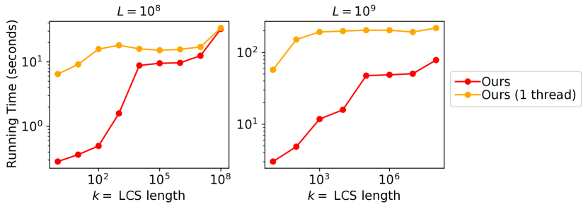
Figure 6. Running time of our parallel LCS algorithm (in Sec. 3).

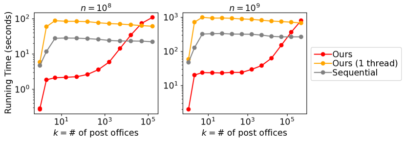
Figure 7. Running time of our parallel convex-GLWS algorithm (Alg. 1).

7   Conclusion and Future Work

We systematically studied general approaches to parallelize classic sequential dynamic programming algorithms, particularly those with non-trivial optimizations such as decision monotonicity and sparsification. We showed a novel framework, the Cordon Algorithm, and apply it to different DP recurrences. Theoretically, we gave the concept of optimal parallelism and perfect parallelism of a sequential algorithm, and showed that with a careful design, we can achieve optimal parallelism for the classic sequential DP algorithms in a (nearly) work-efficient manner, and perfect parallelism for some instances. Practically, we show that our carefully-designed techniques do not include much overhead, and can outperform the original sequential version in a wide variety of cases.

We believe that the novelty of the techniques in this paper opens a list of interesting questions. First, many of the new parallel algorithms are nearly work-efficient—we pick the most practical sequential algorithms for each problem, but they can be off the best work bound by up to an $O(\log n)$ factor. It is theoretically interesting to ask if we can match the best work bound in parallel. Second, among all these classic algorithms we looked at, one problem/algorithm that cannot be directly solved by the Cordon Algorithm is the RNA Secondary Structure (Eppstein et al., 1988). Here, we may have $2^{n}$ different paths in a DP DAG, so applying Cordon Algorithm efficiently may need some complicated techniques. Finally, we show how to faithfully parallelize the sequential DP algorithms. We are aware of other approaches (Lu and Lin, 1994; Tchendji et al., 2020; Xu et al., 2005; Apostolico et al., 1990; Krusche and Tiskin, 2010; Cao et al., 2023) for LIS/LCS that can achieve stronger worst-case span bounds using divide-and-conquer. Hence, an interesting direction is to see if we can redesign other DP algorithms in a similar form to achieve better worst-case span.

Appendix A Additional Details for Parallel Optimal Alphabetic Trees (OAT)

This section supplements additional details for the parallel OAT algorithm in Sec. 5.1.

A.1   Sequential Algorithms for OAT

Hu-Tucker algorithm (Hu and Tucker, 1971) was the first $O(n\log n)$ algorithm for OAT, and a simplified version Garsia-Wachs algorithm (Garsia and Wachs, 1977) was proposed later. Both algorithms have two phases. In the first phase, a certain tree called the $l$-tree (short for level-tree) is constructed from the input sequence. Hu-Tucker algorithm and Garsia-Wachs algorithm differ in the manner to find the $l$-tree, but the final $l$-tree is the same. In the second phase, the OAT can be constructed from the $l$-tree, and each item in the OAT is at the same level as in the $l$-tree.

The key problem is how to compute the $l$-tree. Here we describe the first phase of Garsia-Wachs, as it is easier to understand than Hu-Tucker and the idea is used in the parallel algorithm by Larmore et al. (1993). Let the input weight sequence be $a_{1..n}$. We denote $a_{i}+a_{i+1}$ be the $i$’th 2-sum, for $1\leq i<n$. A pair of consecutive elements $(a_{i},a_{i+1})$ is said to be locally minimal if the $i$’th 2-sum is a local minimum in the sequence of 2-sums. The Garsia-Wachs algorithm repeatedly performs the following steps until there is only one element in the sequence:

1. Find the left-most locally minimal pair $(a_{i},a_{i+1})$.

2. Combine $a_{i}$ and $a_{i+1}$. Make a new node $x$ to be the parent of $a_{i}$ and $a_{i+1}$ in the $l$-tree, and the weight of $x$ is $a_{i}+a_{i+1}$.

3. Remove $a_{i}$ and $a_{i+1}$ from the sequence. Insert $x$ before the first element $a_{j}$ where $j>i$ and $a_{j}\geq x$. If such $a_{j}$ does not exist, insert $x$ at the end of the sequence.

Note that each newly generated node represents a tree, with both children as the two trees corresponding to the two nodes it merges in step (2). At the end, there will be only one element in the sequence, which is the final output of the $l$-tree. An $l$-tree can be easily converted to an OAT in parallel with $O(n)$ work and $O(\log n)$ span, and we refer the audience to (Larmore et al., 1993) for more details.

A.2   The Parallel Algorithm by Larmore et al. (1993)

Here we focus on the first phase on how to construct the $l$-tree in parallel. Larmore et al. observe that we can pick any locally minimal pair instead of the left-most one as in Garsia-Wachs, which does not affect the resulting $l$-tree. Hence, we can in parallel process all possible locally minimal pairs in one round. However, in the worst case the number of rounds is still linear. For example, if $a_{1..n}$ is in increasing order, then only one locally minimal pair can be processed in one round.

To overcome this issue, Larmore et al. further proposed the concept of “valleys”. A valley $\alpha=\mathit{vall}(a_{i})$ is the largest contiguous subsegment of $a$ that 1) contains $a_{i}$, and 2) contains no item larger than $a_{i}$. Hence, $a_{i}$’s valley contains the elements from $a_{i}$’s subtree in the Cartesian tree of $a$. Larmore et al. showed that several disjoint valleys in the sequence can be processed in parallel. To understand this, let us consider a valley $\alpha$. Let $\Delta_{\alpha}$ be the parent of valley $\alpha$ in the Cartesian tree. Since $\alpha$ is maximal, the locally minimal pairs from this range will not interact with the outside elements. Hence, we can consider valley $\alpha$ as an independent task, and repeatedly find and combine the locally minimal pairs inside $\alpha$. The only difference is that if the combined element $x=a_{i}+a_{i+1}>\Delta_{\alpha}$, we mark it as $x^{*}$ and put it in a separate queue. After the parallel processing of disjoint valleys, we collect all marked elements and insert them into the right place.

In total, there can be at most $n$ overlapping valleys. Larmore et al.’s algorithm uses one special type of valley: the 1-valleys. A 1-valley is defined to be a valley $\alpha$ such that for any node $v$ in the subtree of $\alpha$ in the Cartesian tree, if $v$ has two children, at least one of the children is a leaf. We can see that in the sequence the maximal 1-valleys are not overlapping, so we can process them in parallel. They also proved that, in each round if we process all maximal 1-valleys and reinsert them as in the sequential order, the number of maximal 1-valleys in the remaining sequence decreases by at least a half. Thus, the whole algorithm will finish in $O(\log n)$ rounds.

Before we show how to process a 1-valley, we introduce some definitions. Let $p(u)$ is the parent of $u$ in the Cartesian tree of $\alpha$. We define a 1-valley $\alpha$ to be a regular valley if for $u<v$ are two leaves in the Cartesian tree of $\alpha$, then $p(u)<p(v)$. A sorted regular valley is defined as a regular valley with the minimum element in the first one. Larmore et al. showed that a 1-valley can be transformed to a sorted regular valley in $O(m)$ work and $O(\log m)$ span, where $m$ is the size of this 1-valley. A set of items $S$ is defined to be lf-closed (short for leaf-father-closed) if for any $a_{i}\in S$ and $a_{i}$ is a leaf in the Cartesian tree of $\alpha$, then $p(a_{i})$ is also in $S$. The weight of $S$ is defined as the sum of the weights of all items in it. We define $W_{k}$ as the minimum weighted lf-closed set with $k$ items in it. Larmore et al. showed that all $W_{k}$ can be computed in $O(m\log m)$ work and $O(\log m)$ span.

Now consider a sorted regular valley $\alpha$ with length $m$. Our goal is to generate a sequence of forests $\mathit{forest}_{0..m^{\prime}-1}$ ($m^{\prime}<m$) so that each of them corresponds to a subset of subtrees in the $l$-tree. Here $\mathit{forest}_{0}$ is empty. The last forest $\mathit{forest}_{m-1}$, if $m=m^{\prime}$, corresponds to the $l$-tree if we merge all elements in this valley. However, this process may not end here—as mentioned above, we will stop if the weights of subtrees exceed $\Delta_{\alpha}$. Hence, we can have our final state $\mathit{forest}_{m^{\prime}-1}$ with $m^{\prime}<m$. To compute $\mathit{forest}_{i}$, we will enumerate all $\mathit{forest}_{j}$ for $j<i$, and find the best (minimum) transition from them. Here a transition means to build an additional level in the $l$-tree, and the cost $w(j,i)=W_{2i-j}$. Larmore et al. showed that the cost function $w$ is convex, so computing $\mathit{forest}_{i}$ is exactly a convex GLWS problem. If we use Alg. 1 to solve this convex GLWS problem, since each decision $\mathit{best}[i]=j$ will add another level to the trees in $\mathit{forest}_{i}$ from $\mathit{forest}_{j}$, the effective depth is upper bounded by the overall $l$-tree height $h$. Hence, the work and span for each 1-valley subproblem is $O(m\log m)$ work and $O(h\log^{2}m)$ span, where $m$ is the subproblem size. Since the total size of 1-valleys in a recursive round is $O(n)$, the work and span for one round are $O(n\log n)$ work and $O(h\log^{2}n)$, respectively. Multiplying this by $O(\log n)$, the number of recursive rounds, gives the cost bounds in Thm. 5.1.

A.3   Proof of Lemma 5.2

Here we provide the proof of Lemma 5.2. We first show the following lemma.

Lemma A.0.

Let the weight of a subtree in an OAT as the total weight of all leaves in this subtree. In an OAT, the subtree weight grows by at least twice for every three levels.

• Here we denote $p(v)$ as the parent node of $v$ in the output OAT $T$ and $w(v)$ as the sum of the leaf weights in the subtree of node $v$. We will show for any node $a$ in the OAT, the great-grandfather of $a$ (if exists) must have weight no less than $2w(a)$. In the optimal alphabetic tree $T$, let node $b$ be $a$’s sibling and node $c$ be $a$’s parent. WLOG we assume node $a$ is the left child of node $c$. Then, let $d$ be $c$’s sibling, $e$ as $c$’s parent, and $f$ as $e$’s parent. Now the lemma is equivalent to $w(f)\geq 2w(a)$.

  We consider the first case when $c$ is $e$’s left child (case 1 in Fig. 8). In this case, we must have $w(d)\geq w(a)$, since otherwise a right rotation will decrement the total cost of the tree by $w(d)-w(a)$, violating that $T$ is an OAT. Hence, $w(f)\geq w(e)\geq w(d)+w(a)\geq 2w(a)$ in this case.

  The second case is when $c$ is $e$’s right child. There are two sub-cases. First, if $e$ is $f$’s right child (case 2(a) in Fig. 8), then $c$, $e$, and $f$ form another case 1. Hence, we have $w(f)\geq 2w(c)\geq 2w(a)$. Second, if $e$ is $f$’s left child (see $T_{4}$ in case 2(b) in Fig. 8). We can double-rotate and get another valid alphabetic tree $T_{5}$. As $T_{4}$ is the optimal alphabetic tree, we must have $2w(d)+3w(a)+3w(b)+w(g)\leq 2(w(d)+w(a)+w(b)+w(g))$, which leads to $w(g)\geq w(a)+w(b)$. So $w(f)=w(d)+w(a)+w(b)+w(g)\geq w(a)+w(g)\geq 2w(a)$.

  From all three cases above, we show $w(f)\geq 2w(a)$, which proves the lemma that the weight doubles for every three steps up the OAT. ∎

With integer weights in word size $W$, the weight of the root is at most $O(W)$, and the weight of each leaf is at least 1. In this case, the number of levels between them is at most $O(\log W)$. This proves Lemma 5.2.

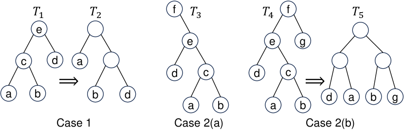
Figure 8. Illustrations for analyzing the OAT Height. The three cases are used in the proof of Lemma A.1.

References

- (1)
- Aggarwal and Klawe (1990) Alok Aggarwal and Maria Klawe. 1990. Applications of generalized matrix searching to geometric algorithms. Discrete Applied Mathematics 27, 1-2 (1990), 3–23.
- Aggarwal et al. (1987) Alok Aggarwal, Maria M Klawe, Shlomo Moran, Peter Shor, and Robert Wilber. 1987. Geometric applications of a matrix-searching algorithm. Algorithmica 2, 1 (1987), 195–208.
- Aimone et al. (2019) James B Aimone, Ojas Parekh, Cynthia A Phillips, Ali Pinar, William Severa, and Helen Xu. 2019. Dynamic programming with spiking neural computing. In International Conference on Neuromorphic Systems. 1–9.
- Alok and James ([n.d.]) Aggarwal Alok and Park James. [n.d.]. Notes on searching in multidimensional monotone arrays. In IEEE Symposium on Foundations of Computer Science (FOCS). 497–512.
- Alves et al. (2002) Carlos ER Alves, Edson Norberto Cáceres, and FKHA Dehne. 2002. Parallel dynamic programming for solving the string editing problem on a CGM/BSP. In ACM Symposium on Parallelism in Algorithms and Architectures (SPAA). 275–281.
- Apostolico et al. (1990) Alberto Apostolico, Mikhail J Atallah, Lawrence L Larmore, and Scott McFaddin. 1990. Efficient parallel algorithms for string editing and related problems. SIAM J. on Computing 19, 5 (1990), 968–988.
- Apostolico and Guerra (1987) Alberto Apostolico and Concettina Guerra. 1987. The longest common subsequence problem revisited. Algorithmica 2 (1987), 315–336.
- Arora et al. (2001) Nimar S Arora, Robert D Blumofe, and C Greg Plaxton. 2001. Thread scheduling for multiprogrammed multiprocessors. Theory of Computing Systems (TOCS) 34, 2 (2001), 115–144.
- Atallah et al. (1989) Mikhail J Atallah, S Rao Kosaraju, Lawrence L Larmore, Gary L Miller, and S-H Teng. 1989. Constructing trees in parallel. In ACM Symposium on Parallelism in Algorithms and Architectures (SPAA). 421–431.
- Awan et al. (2020) Muaaz G Awan, Jack Deslippe, Aydin Buluc, Oguz Selvitopi, Steven Hofmeyr, Leonid Oliker, and Katherine Yelick. 2020. ADEPT: a domain independent sequence alignment strategy for gpu architectures. BMC bioinformatics 21, 1 (2020), 1–29.
- Babu and Saxena (1997) K Nandan Babu and Sanjeev Saxena. 1997. Parallel algorithms for the longest common subsequence problem. In IEEE International Conference on High Performance Computing (HiPC). IEEE, 120–125.
- Bateni et al. (2018) MohammadHossein Bateni, Soheil Behnezhad, Mahsa Derakhshan, MohammadTaghi Hajiaghayi, and Vahab Mirrokni. 2018. Massively parallel dynamic programming on trees. arXiv preprint arXiv:1809.03685 (2018).
- Bellman (1954) Richard Bellman. 1954. The theory of dynamic programming. Bull. Amer. Math. Soc. 60, 6 (1954), 503–515.
- Blelloch et al. (2022) Guy Blelloch, Daniel Ferizovic, and Yihan Sun. 2022. Joinable Parallel Balanced Binary Trees. ACM Transactions on Parallel Computing (TOPC) 9, 2 (2022), 1–41.
- Blelloch et al. (2020a) Guy E. Blelloch, Daniel Anderson, and Laxman Dhulipala. 2020a. ParlayLib — a toolkit for parallel algorithms on shared-memory multicore machines. In ACM Symposium on Parallelism in Algorithms and Architectures (SPAA). 507–509.
- Blelloch et al. (2016a) Guy E. Blelloch, Daniel Ferizovic, and Yihan Sun. 2016a. Just Join for Parallel Ordered Sets. In ACM Symposium on Parallelism in Algorithms and Architectures (SPAA).
- Blelloch et al. (2020b) Guy E. Blelloch, Jeremy T. Fineman, Yan Gu, and Yihan Sun. 2020b. Optimal parallel algorithms in the binary-forking model. In ACM Symposium on Parallelism in Algorithms and Architectures (SPAA). 89–102.
- Blelloch and Gu (2020) Guy E. Blelloch and Yan Gu. 2020. Improved Parallel Cache-Oblivious Algorithms for Dynamic Programming. In SIAM Symposium on Algorithmic Principles of Computer Systems (APOCS).
- Blelloch et al. (2016b) Guy E. Blelloch, Yan Gu, Yihan Sun, and Kanat Tangwongsan. 2016b. Parallel Shortest Paths Using Radius Stepping. In ACM Symposium on Parallelism in Algorithms and Architectures (SPAA). 443–454.
- Blumofe and Leiserson (1999) Robert D. Blumofe and Charles E. Leiserson. 1999. Scheduling multithreaded computations by work stealing. J. ACM 46, 5 (1999), 720–748.
- Boroujeni and Seddighin (2019) Mahdi Boroujeni and Saeed Seddighin. 2019. Improved MPC algorithms for edit distance and Ulam distance. In ACM Symposium on Parallelism in Algorithms and Architectures (SPAA). 31–40.
- Bradford et al. (1998) Phillip G Bradford, Gregory JE Rawlins, and Gregory E Shannon. 1998. Efficient matrix chain ordering in polylog time. SIAM J. on Computing 27, 2 (1998), 466–490.
- Cao et al. (2023) Nairen Cao, Shang-En Huang, and Hsin-Hao Su. 2023. Nearly optimal parallel algorithms for longest increasing subsequence. In ACM Symposium on Parallelism in Algorithms and Architectures (SPAA).
- Chan and Lam (1990) Kwong-fai Chan and Tak-wah Lam. 1990. Finding least-weight subsequences with fewer processors. In International Symposium on Algorithms. Springer, 318–327.
- Chen et al. (2006) Yixin Chen, Andrew Wan, and Wei Liu. 2006. A fast parallel algorithm for finding the longest common sequence of multiple biosequences. BMC bioinformatics 7 (2006), 1–12.
- Chowdhury et al. (2016) Rezaul Chowdhury, Pramod Ganapathi, Jesmin Jahan Tithi, Charles Bachmeier, Bradley C Kuszmaul, Charles E Leiserson, Armando Solar-Lezama, and Yuan Tang. 2016. Autogen: Automatic discovery of cache-oblivious parallel recursive algorithms for solving dynamic programs. In ACM Symposium on Principles and Practice of Parallel Programming (PPOPP). 10.
- Chowdhury and Ramachandran (2006) Rezaul A. Chowdhury and Vijaya Ramachandran. 2006. Cache-oblivious dynamic programming. In ACM-SIAM Symposium on Discrete Algorithms (SODA). 591–600.
- Chowdhury and Ramachandran (2008) Rezaul A. Chowdhury and Vijaya Ramachandran. 2008. Cache-efficient dynamic programming algorithms for multicores. In ACM Symposium on Parallelism in Algorithms and Architectures (SPAA). ACM.
- Chowdhury and Ramachandran (2010) Rezaul A. Chowdhury and Vijaya Ramachandran. 2010. The cache-oblivious gaussian elimination paradigm: theoretical framework, parallelization and experimental evaluation. Theory of Computing Systems (TOCS) 47, 4 (2010), 878–919.
- Czumaj (1992) Artur Czumaj. 1992. Parallel algorithm for the matrix chain product problem. (1992).
- Davis (1998) Sashka Davis. 1998. Hu-Tucker alogorithm for building optimal alphabetic binary search trees. (1998).
- Ding et al. (2023) Xiangyun Ding, Xiaojun Dong, Yan Gu, Youzhe Liu, and Yihan Sun. 2023. Efficient Parallel Output-Sensitive Edit Distance. In 31st Annual European Symposium on Algorithms (ESA 2023) (Leibniz International Proceedings in Informatics (LIPIcs)), Inge Li Gørtz, Martin Farach-Colton, Simon J. Puglisi, and Grzegorz Herman (Eds.), Vol. 274. Schloss Dagstuhl – Leibniz-Zentrum für Informatik, Dagstuhl, Germany, 40:1–40:20. https://doi.org/10.4230/LIPIcs.ESA.2023.40
- Ding et al. (2024) Xiangyun Ding, Yan Gu, and Yihan Sun. 2024. Source Code. https://github.com/ucrparlay/Parallel-Work-Efficient-Dynamic-Programming.
- Driscoll et al. (1989) James R. Driscoll, Neil Sarnak, Daniel D. Sleator, and Robert E. Tarjan. 1989. Making data structures persistent. J. Computer and System Sciences 38, 1 (1989), 86–124.
- Eppstein (1990) David Eppstein. 1990. Sequence comparison with mixed convex and concave costs. J. Algorithms 11, 1 (1990), 85–101.
- Eppstein et al. (1988) David Eppstein, Zvi Galil, and Raffaele Giancarlo. 1988. Speeding up dynamic programming. In IEEE Symposium on Foundations of Computer Science (FOCS). 488–496.
- Eppstein et al. (1990) David Eppstein, Zvi Galil, Raffaele Giancarlo, and Giuseppe F Italiano. 1990. Sparse dynamic programming. In ACM-SIAM Symposium on Discrete Algorithms (SODA). 513–522.
- Eppstein et al. (1992a) David Eppstein, Zvi Galil, Raffaele Giancarlo, and Giuseppe F Italiano. 1992a. Sparse dynamic programming I: linear cost functions. J. ACM 39, 3 (1992), 519–545.
- Eppstein et al. (1992b) David Eppstein, Zvi Galil, Raffaele Giancarlo, and Giuseppe F Italiano. 1992b. Sparse dynamic programming II: convex and concave cost functions. J. ACM 39, 3 (1992), 546–567.
- Galil and Giancarlo (1989) Zvi Galil and Raffaele Giancarlo. 1989. Speeding up dynamic programming with applications to molecular biology. Theoretical Computer Science (TCS) 64, 1 (1989), 107–118.
- Galil and Park (1989) Zvi Galil and Kunsoo Park. 1989. A linear-time algorithm for concave one-dimensional dynamic programming. (1989).
- Galil and Park (1992) Zvi Galil and Kunsoo Park. 1992. Dynamic programming with convexity, concavity and sparsity. Theoretical Computer Science 92, 1 (1992), 49–76.
- Galil and Park (1994) Zvi Galil and Kunsoo Park. 1994. Parallel algorithms for dynamic programming recurrences with more than O(1) dependency. J. Parallel Distrib. Comput. 21, 2 (1994), 213–222.
- Garsia and Wachs (1977) Adriano M Garsia and Michelle L Wachs. 1977. A new algorithm for minimal binary search trees. SIAM J. Comput. 6, 4 (1977), 622–642.
- Gu et al. (2023) Yan Gu, Ziyang Men, Zheqi Shen, Yihan Sun, and Zijin Wan. 2023. Parallel Longest Increasing Subsequence and van Emde Boas Trees. In ACM Symposium on Parallelism in Algorithms and Architectures (SPAA).
- Gu et al. (2022) Yan Gu, Zachary Napier, and Yihan Sun. 2022. Analysis of Work-Stealing and Parallel Cache Complexity. In SIAM Symposium on Algorithmic Principles of Computer Systems (APOCS). SIAM, 46–60.
- Gupta et al. (2023) Chetan Gupta, Rustam Latypov, Yannic Maus, Shreyas Pai, Simo Särkkä, Jan Studenỳ, Jukka Suomela, Jara Uitto, and Hossein Vahidi. 2023. Fast Dynamic Programming in Trees in the MPC Model. In ACM Symposium on Parallelism in Algorithms and Architectures (SPAA). 443–453.
- Hirschberg (1977) Daniel S Hirschberg. 1977. Algorithms for the longest common subsequence problem. J. ACM 24, 4 (1977), 664–675.
- Hirschberg and Larmore (1987) Daniel S Hirschberg and Lawrence L. Larmore. 1987. The least weight subsequence problem. SIAM J. on Computing 16, 4 (1987), 628–638.
- Hu and Tucker (1971) Te C Hu and Alan C Tucker. 1971. Optimal computer search trees and variable-length alphabetical codes. SIAM J. Appl. Math. 21, 4 (1971), 514–532.
- Huang et al. (1994) S-HS Huang, Hongfei Liu, and Venkatraman Viswanathan. 1994. Parallel dynamic programming. IEEE International Parallel and Distributed Processing Symposium (IPDPS) 5, 3 (1994), 326–328.
- Huffman (1952) David A. Huffman. 1952. A method for the construction of minimum-redundancy codes. Proceedings of the IRE 40, 9 (1952), 1098–1101.
- Hunt and Szymanski (1977) James W Hunt and Thomas G Szymanski. 1977. A fast algorithm for computing longest common subsequences. Commun. ACM 20, 5 (1977), 350–353.
- Im et al. (2017) Sungjin Im, Benjamin Moseley, and Xiaorui Sun. 2017. Efficient massively parallel methods for dynamic programming. In ACM Symposium on Theory of Computing (STOC). 798–811.
- Itai (1976) Alon Itai. 1976. Optimal alphabetic trees. SIAM J. Comput. 5, 1 (1976), 9–18.
- Itzhaky et al. (2016) Shachar Itzhaky, Rohit Singh, Armando Solar-Lezama, Kuat Yessenov, Yongquan Lu, Charles Leiserson, and Rezaul Chowdhury. 2016. Deriving divide-and-conquer dynamic programming algorithms using solver-aided transformations. In Symposium on Object-oriented Programming, Systems, Languages and Applications (OOPSLA). 145–164.
- Javanmard et al. (2019) Mohammad Mahdi Javanmard, Pramod Ganapathr, Rathish Das, Zafar Ahmad, Stephen Tschudi, and Rezaul Chowdhury. 2019. Toward efficient architecture-independent algorithms for dynamic programs: poster. In Symposium on Principles and Practice of Parallel Programming (PPoPP). 413–414.
- Karpinski et al. (1997) Marek Karpinski, Lawrence L Larmore, and Wojciech Rytter. 1997. Correctness of constructing optimal alphabetic trees revisited. Theoretical Computer Science 180, 1-2 (1997), 309–324.
- Klawe (1989) Maria M. Klawe. 1989. A simple linear time algorithm for concave one-dimensional dynamic programming. University of British Columbia Vancouver.
- Klawe and Kleitman (1990) Maria M Klawe and Daniel J Kleitman. 1990. An almost linear time algorithm for generalized matrix searching. SIAM Journal on Discrete Mathematics 3, 1 (1990), 81–97.
- Knuth (1971) Donald E. Knuth. 1971. Optimum binary search trees. Acta informatica 1 (1971), 14–25.
- Knuth (1973) Donald E. Knuth. 1973. The Art of Computer Programming, Volume III: Sorting and Searching. Addison-Wesley.
- Knuth and Plass (1981) Donald E. Knuth and Michael F. Plass. 1981. Breaking paragraphs into lines. Software: Practice and Experience 11, 11 (1981), 1119–1184.
- Krusche and Tiskin (2009) Peter Krusche and Alexander Tiskin. 2009. Parallel longest increasing subsequences in scalable time and memory. In International Conference on Parallel Processing and Applied Mathematics. Springer, 176–185.
- Krusche and Tiskin (2010) Peter Krusche and Alexander Tiskin. 2010. New algorithms for efficient parallel string comparison. In ACM Symposium on Parallelism in Algorithms and Architectures (SPAA). 209–216.
- Larmore and Przytycka (1995) Lawrence L Larmore and Teresa M Przytycka. 1995. Constructing Huffman trees in parallel. SIAM J. on Computing 24, 6 (1995), 1163–1169.
- Larmore and Przytycka (1996) Lawrence L Larmore and Teresa M Przytycka. 1996. A parallel algorithm for optimum height-limited alphabetic binary trees. J. Parallel and Distrib. Comput. 35, 1 (1996), 49–56.
- Larmore and Przytycka (1998) Lawrence L Larmore and Teresa M Przytycka. 1998. The optimal alphabetic tree problem revisited. Journal of Algorithms 28, 1 (1998), 1–20.
- Larmore et al. (1993) Lawrence L Larmore, Teresa M Przytycka, and Wojciech Rytter. 1993. Parallel construction of optimal alphabetic trees. In ACM symposium on Parallel Algorithms and Architectures (SPAA). 214–223.
- Larmore and Rytter (1994) Lawrence L Larmore and Wojciech Rytter. 1994. An optimal sublinear time parallel algorithm for some dynamic programming problems. Inform. Process. Lett. 52, 1 (1994), 31–34.
- Larmore and Schieber (1991) Lawrence L Larmore and Baruch Schieber. 1991. On-line dynamic programming with applications to the prediction of RNA secondary structure. J. Algorithms 12, 3 (1991), 490–515.
- Li et al. (2014) Xiang Li, Jiahua Wei, Tiejian Li, Guangqian Wang, and William W-G Yeh. 2014. A parallel dynamic programming algorithm for multi-reservoir system optimization. Advances in water resources 67 (2014), 1–15.
- Lu and Lin (1994) Mi Lu and Hua Lin. 1994. Parallel algorithms for the longest common subsequence problem. IEEE Transactions on Parallel and Distributed Systems 5, 8 (1994), 835–848.
- Miller and Myers (1988) Webb Miller and Eugene W Myers. 1988. Sequence comparison with concave weighting functions. Bulletin of mathematical biology 50 (1988), 97–120.
- Monge (1781) Gaspard Monge. 1781. Mémoire sur la théorie des déblais et des remblais. Mem. Math. Phys. Acad. Royale Sci. (1781), 666–704.
- Nagaraj (1997) SV Nagaraj. 1997. Optimal binary search trees. Theoretical Computer Science 188, 1-2 (1997), 1–44.
- Rytter (1988) Wojciech Rytter. 1988. On efficient parallel computations for some dynamic programming problems. Theoretical Computer Science 59, 3 (1988), 297–307.
- Shen et al. (2022) Zheqi Shen, Zijin Wan, Yan Gu, and Yihan Sun. 2022. Many Sequential Iterative Algorithms Can Be Parallel and (Nearly) Work-efficient. In ACM Symposium on Parallelism in Algorithms and Architectures (SPAA).
- Sleator and Tarjan (1983) Daniel D Sleator and Robert Endre Tarjan. 1983. A data structure for dynamic trees. J. Computer and System Sciences 26, 3 (1983), 362–391.
- Sun and Blelloch (2019) Yihan Sun and Guy E Blelloch. 2019. Parallel Range, Segment and Rectangle Queries with Augmented Maps. In SIAM Symposium on Algorithm Engineering and Experiments (ALENEX). 159–173.
- Sun et al. (2018) Yihan Sun, Daniel Ferizovic, and Guy E Blelloch. 2018. PAM: Parallel Augmented Maps. In ACM Symposium on Principles and Practice of Parallel Programming (PPOPP).
- Tang and Wang (2017) Yuan Tang and Shiyi Wang. 2017. Brief Announcement: STAR (Space-Time Adaptive and Reductive) Algorithms for Dynamic Programming Recurrences with More Than O(1) Dependency. In ACM Symposium on Parallelism in Algorithms and Architectures (SPAA). 279–281.
- Tang et al. (2015) Yuan Tang, Ronghui You, Haibin Kan, Jesmin Jahan Tithi, Pramod Ganapathi, and Rezaul A Chowdhury. 2015. Cache-oblivious wavefront: improving parallelism of recursive dynamic programming algorithms without losing cache-efficiency. In ACM Symposium on Principles and Practice of Parallel Programming (PPOPP). 205–214.
- Tchendji et al. (2020) Vianney Kengne Tchendji, Armel Nkonjoh Ngomade, Jerry Lacmou Zeutouo, and Jean Frédéric Myoupo. 2020. Efficient CGM-based parallel algorithms for the longest common subsequence problem with multiple substring-exclusion constraints. Parallel Comput. 91 (2020), 102598.
- Tithi et al. (2015) Jesmin Jahan Tithi, Pramod Ganapathi, Aakrati Talati, Sonal Aggarwal, and Rezaul Chowdhury. 2015. High-performance energy-efficient recursive dynamic programming with matrix-multiplication-like flexible kernels. In IEEE International Parallel and Distributed Processing Symposium (IPDPS). 303–312.
- Vahidi et al. (2023) Soroush Vahidi, Baruch Schieber, Zhihui Du, and David A Bader. 2023. Parallel Longest Common SubSequence Analysis In Chapel. In 2023 IEEE High Performance Extreme Computing Conference (HPEC). IEEE, 1–6.
- Van Leeuwen (1976) Jan Van Leeuwen. 1976. On the Construction of Huffman Trees. In ICALP. 382–410.
- Wang and Song (2011) Haizhou Wang and Mingzhou Song. 2011. Ckmeans. 1d. dp: optimal k-means clustering in one dimension by dynamic programming. The R journal 3, 2 (2011), 29.
- Weiss and Schwartz (2019) Elad Weiss and Oded Schwartz. 2019. Computation of Matrix Chain Products on Parallel Machines. In International Parallel and Distributed Processing Symposium (IPDPS). IEEE, 491–500.
- Wilber (1988) Robert Wilber. 1988. The concave least-weight subsequence problem revisited. J. Algorithms 9, 3 (1988), 418–425.
- Xu et al. (2005) Xiaohua Xu, Ling Chen, Yi Pan, and Ping He. 2005. Fast parallel algorithms for the longest common subsequence problem using an optical bus. In International Conference on Computational Science and Its Applications. Springer, 338–348.
- Yang et al. (2022) Dingcheng Yang, Wenjian Yu, Xiangyun Ding, Ao Zhou, and Xiaoyi Wang. 2022. DP-Nets: Dynamic programming assisted quantization schemes for DNN compression and acceleration. Integration 82 (2022), 147–154.
- Yao (1980) F. Frances Yao. 1980. Efficient dynamic programming using quadrangle inequalities. In ACM Symposium on Theory of Computing (STOC). 429–435.
- Yao (1982) F Frances Yao. 1982. Speed-up in dynamic programming. SIAM Journal on Algebraic Discrete Methods 3, 4 (1982), 532–540.