3D Guidance Law for Maximal Coverage and Target Enclosing with Inherent Safety

Abstract

In this paper, we address the problem of enclosing an arbitrarily moving target in three dimensions by a single pursuer, which is an unmanned aerial vehicle (UAV), for maximum coverage while also ensuring the pursuer’s safety by preventing collisions with the target. The proposed guidance strategy steers the pursuer to a safe region of space surrounding the target, allowing it to maintain a certain distance from the latter while offering greater flexibility in positioning and converging to any orbit within this safe zone. Our approach is distinguished by the use of nonholonomic constraints to model vehicles with accelerations serving as control inputs and coupled engagement kinematics to craft the pursuer’s guidance law meticulously. Furthermore, we leverage the concept of Lyapunov Barrier Function as a powerful tool to constrain the distance between the pursuer and the target within asymmetric bounds, thereby ensuring the pursuer’s safety within the predefined region. To validate the efficacy and robustness of our algorithm, we conduct experimental tests by implementing a high-fidelity quadrotor model within Software-in-the-loop (SITL) simulations, encompassing various challenging target maneuver scenarios. The results obtained showcase the resilience of the proposed guidance law, effectively handling arbitrarily maneuvering targets, vehicle/autopilot dynamics, and external disturbances. Our method consistently delivers stable global enclosing behaviors, even in response to aggressive target maneuvers, and requires only relative information for successful execution.

I Introduction

In recent times, autonomous vehicles have gained significant prominence in a range of tasks, including reconnaissance, surveillance, crop and forest monitoring, and search and rescue missions [1, 2, 3, 4, 5]. Most of these tasks share a common theme of behavior where an autonomous vehicle known as the pursuer monitors an object of interest known as the target. The pursuer achieves this by maintaining a specific distance or proximity to the target, which can be stationary or dynamic. The pursuer’s ability to achieve a stable motion around the target, thereby maintaining fixed desired proximity, is commonly referred to as target enclosing, target circumnavigation, or target encirclement [6]. One of the earliest approaches to address the target enclosing problem involved utilizing cyclic pursuit by agents to achieve a circular formation around the target [7, 8]. In another approach known as vector field guidance, the pursuer enclosed the target utilizing vector fields designed to create a limit cycle or a periodic orbit of the desired shape around the target [9, 10, 11, 12, 13]. Several other methods have been developed for trapping one or more targets in circular orbits based on different guidance strategies while also focusing on reducing the communication effort [14, 15, 16, 17, 18, 19]. For example, only range measurements were utilized in [15], while only bearing information was utilized in [14, 16]. In [18, 19], only relative information (range and bearing measurements) was utilized for the development of target encirclement laws, whereas the work in [6, 20, 21, 22, 23, 24] addressed a general target enclosing problem using relative information.

The above-mentioned works developed target enclosing laws with restrictions on the target’s motion (stationary or slow-moving target). Such simplifications make it possible to obtain a tractable feedback controller but may require information on the target maneuver, necessitating communication between the target and the pursuer. For example, in [25], the authors assumed the target to be moving in a straight line, while the authors in [19] developed separate laws when dealing with constant acceleration, constant velocity, or stationary target. Further, despite the practical importance of 3D engagements, there has been limited focus on the development of laws for target enclosing in 3D space. In [26], authors utilized a behavioral model to develop a 3D guidance algorithm to enclose a target in a GPS-denied environment based on camera images. The authors in [27] developed target tracking laws for a pursuer with nonholonomic kinematics, orbiting on a path depending on the target’s heading and motion, and provided experimental results for an actual airship. Further, the above-mentioned works on 3D target enclosing decouple the 3D engagement into two planar engagements, restricting the movement of the pursuer to a single plane and developing guidance laws for simple target maneuvers. Such considerations may depreciate the performance of the guidance law by restricting the allowable path taken by the pursuer. Recently, the works in [21, 22] have developed 3D guidance laws to enclose targets within arbitrary shapes, providing flexibility to the pursuer to move freely.

In most of the previously mentioned works, the authors are primarily concerned with the pursuer reaching the desired proximity around the target. However, to maximize coverage in challenging situations, e.g., in environmental monitoring and surveillance, a robust guidance strategy must allow the pursuer to converge within a predefined region in the vicinity of the desired proximity rather than aiming for a singular orbit. Moreover, in practice, the pursuer may not be able to precisely track its position at the desired proximity due to unmodeled dynamics, disturbances, or aggressive target maneuvers, which may lead to a potential collision between the pursuer and the target. By ensuring the target’s position and the region to which the pursuer converges never intersect, the pursuer’s safety in the designated region (a volume of cloud around the target) can be guaranteed. Additionally, this may provide the pursuer with multiple trajectory options while enclosing the target, eventually leading to maximal coverage and enclosing.

This letter is motivated by the need to develop a generalized 3D target enclosing law for the pursuer that provides safety guarantees and robustness against any target maneuvers while also ensuring maximal coverage. Particularly, our guidance approach steers the pursuer to a region of safe space to develop guidance laws using 3D relative kinematics with nonholonomic constraints without small angle approximations or decoupling to allow greater maneuverability to the pursuer’s motion. Unlike previous approaches, our work provides greater flexibility to the pursuer to execute 3D maneuvers without being restricted to a single plane, requires only relative information, and guarantees its safety from the target. Additionally, we optimally allocate the control effort into the pitch and the yaw planes to minimize the pursuer’s overall energy expenditure during enclosing. Further, we implement our proposed control law on a high-fidelity UAV model via software in the loop simulation to attest to the practicality of our guidance law.

II Problem Formulation

Consider the three-dimensional engagement between a pursuer (P) and a target (T) in the inertial frame of reference $F_{I}$ (denoted by mutually orthogonal $\{X_{I},Y_{I},Z_{I}\}$ axes), as illustrated in the Figure 1(a). The pursuer and the target can move at different speeds, denoted by $V_{P}$ and $V_{T}$, respectively, while they are separated by a distance $r$. By rotating $F_{I}$ through azimuth line-of-sight (LOS) angle $\psi\in(-\pi,\pi]$ and elevation LOS angle $\theta\in[-\pi/2,\pi/2]$, we obtain the pursuer-target LOS frame of reference $F_{L}$, denoted by mutually orthogonal $\{X_{L},Y_{L},Z_{L}\}$ axes. $F_{L}$ has the $X_{L}$ axis aligned along the line-of-sight (LOS) from the pursuer to the target. Further, the body-fixed frame of reference for the pursuer and target are denoted by $F_{P}$ and $F_{T}$, respectively (denoted by mutually orthogonal $\{X_{i},Y_{i},Z_{i}\}$ axes where $i\in\{P,T\}$ represents the pursuer and the target). The engagement between the vehicles in $F_{L}$ is depicted in Figure 1(b), where $V_{P}$ and $V_{T}$ are aligned along the $X_{i}$ axis of their respective body-fixed frame. $F_{P}$ is determined by rotation of $F_{L}$ through pursuer azimuth angle $\chi_{P}\in(-\pi,\pi]$ and pursuer elevation angles $\gamma_{P}\in[-\pi/2,\pi/2]$, while $F_{T}$ is obtained by rotation of $F_{L}$ through pursuer azimuth angle $\chi_{T}\in(-\pi,\pi]$ and pursuer elevation angles $\gamma_{T}\in[-\pi/2,\pi/2]$.

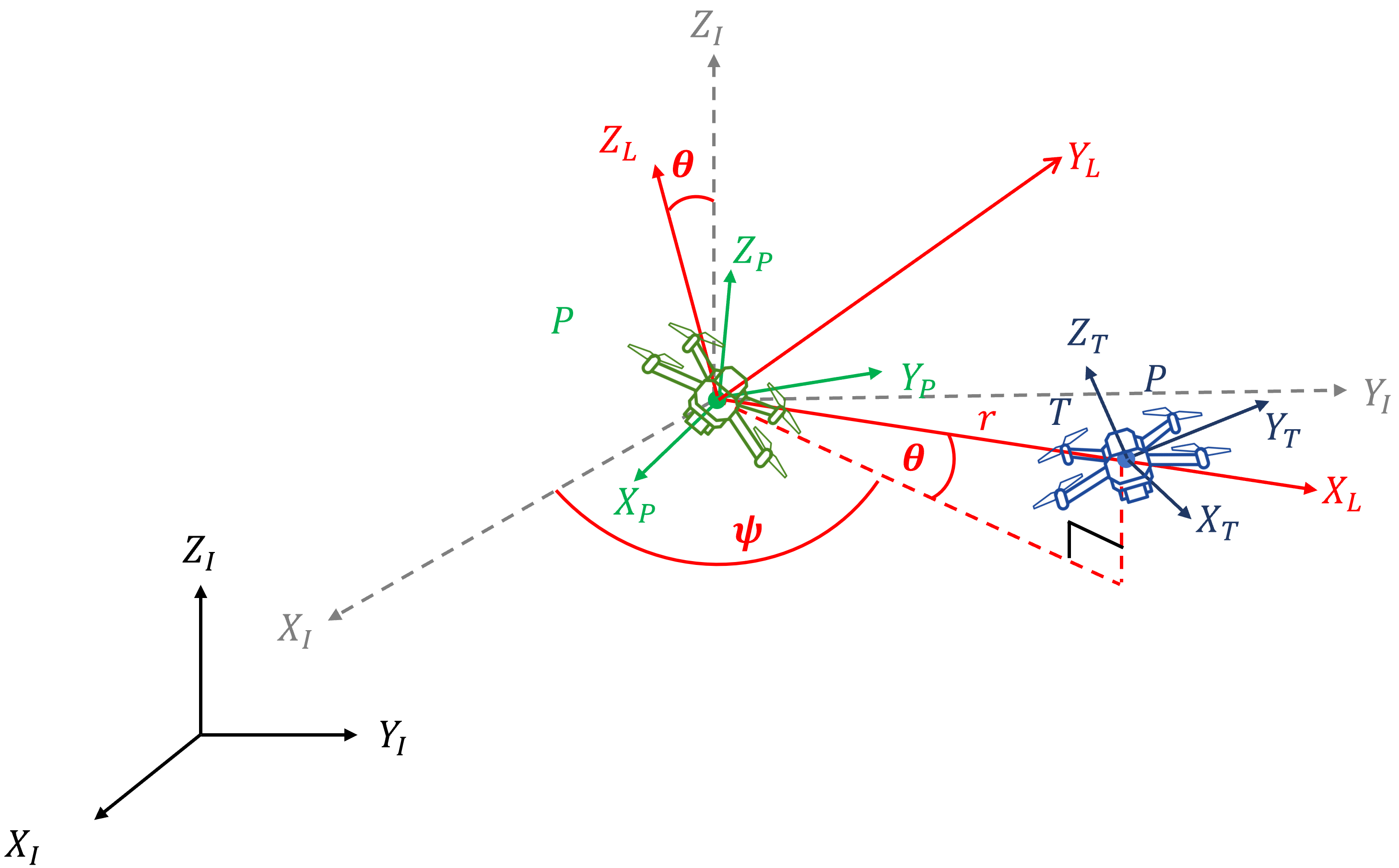
(a) Inertial frame of reference.

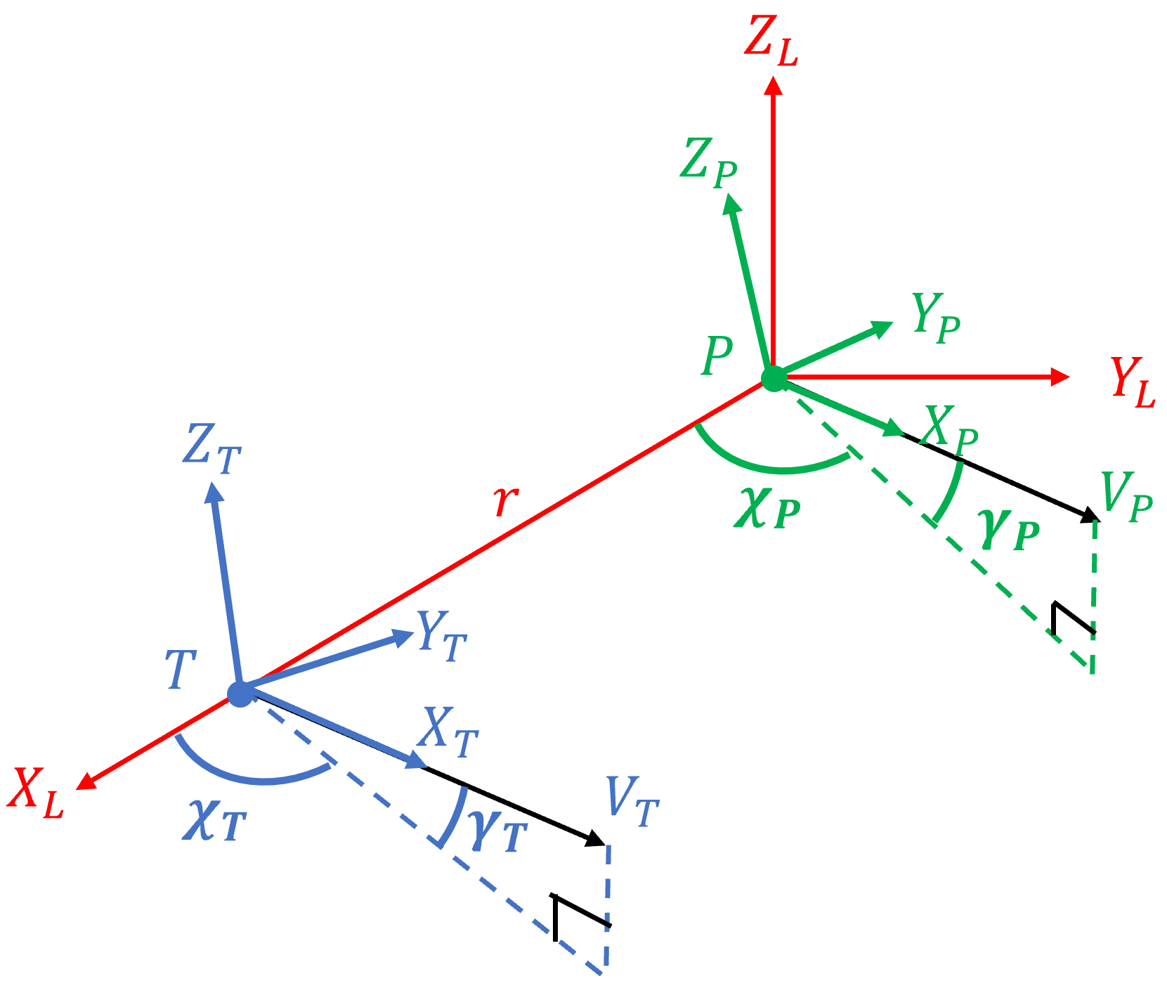
(b) LOS frame of reference.

Figure 1: Engagement geometry.

Assuming the vehicles to be point masses with nonholonomic constraints, the equations of the relative motion between the pursuer and the target are governed by,

$$\dot{r} =V_{T}\cos\gamma_{T}\cos\chi_{T}-V_{P}\cos\gamma_{P}\cos\chi_{P},$$ (1a)

$$\dot{\theta} =\frac{V_{T}\sin\gamma_{T}-V_{P}\sin\gamma_{P}}{r},$$ (1b)

$$\dot{\psi} =\frac{V_{T}\cos\gamma_{T}\sin\chi_{T}-V_{P}\cos\gamma_{P}\sin\chi_{P}}{r\cos\theta},$$ (1c)

where $[V_{i},\gamma_{i}$, $\chi_{i}]^{\top}$ represent the states of the respective vehicle. The rates of the vehicles’ speed and turn are related as follows:

$$\dot{\gamma}_{i} =\frac{a_{i}^{\gamma}}{V_{i}}-\dot{\psi}\sin\theta\sin\chi_{i}-\dot{\theta}\cos\chi_{i},$$ (2a)

$$\dot{\chi}_{i} =\frac{a_{i}^{\chi}}{V_{P}\cos\gamma_{i}}+\dot{\psi}\tan\gamma_{i}\cos\chi_{i}\sin\theta-\dot{\psi}\cos\theta$$

$$-\dot{\theta}\tan\gamma_{i}\sin\chi_{i},$$ (2b)

$$\dot{V}_{i} =a_{i}^{r},$$ (2c)

where $a_{i}^{r}$ denotes the vehicle’s radial acceleration, $a_{i}^{\gamma}$ denotes the lateral acceleration component in the pitch plane, and $a_{i}^{\chi}$ denotes the lateral acceleration component of the vehicles in the yaw plane such that the subscript $i\in\{P,T\}$. The accelerations $\mathbf{u}_{T}=[a_{T}^{r},a_{T}^{\gamma},a_{T}^{\chi}]^{\top}$ and $\mathbf{u}_{P}=[a_{P}^{r},a_{P}^{\gamma},a_{P}^{\chi}]^{\top}$ represent their respective control inputs in their respective body-fixed frames $F_{P}$ and $F_{T}$. As evident from (2c), the radial accelerations $a_{i}^{r}$ directly influence the vehicles’ speeds, while the lateral acceleration components $a_{i}^{\gamma}$ and $a_{i}^{\chi}$ affect their turn rates, thereby influencing the direction of their velocities, as observed in (2a)-(2c). Such a model provides a practical representation for aerial vehicles constrained to steer with a minimum turning radius and controlled through accelerations.The accelerations of the target are assumed to be bounded, that is, $|a_{T}^{r}|\leq a_{\max}^{r}$, $|a_{T}^{\gamma}|\leq a_{\max}^{\gamma}$ and $|a_{T}^{\chi}|\leq a_{\max}^{\chi}$, which is reasonable in practice. It is also crucial to emphasize that the kinematics described in (1) is solely based on relative variables. Such an approach is particularly advantageous in GPS-denied environments, as it relies exclusively on relative measurements. Hence, we assume that the pursuer is equipped with onboard sensors to collect relative information. This setup eliminates the necessity for costly vehicle-to-vehicle communication and allows us to design an algorithm that operates effectively with limited information.

Our objective is to design the control inputs for the pursuer to enclose a mobile target with maximal coverage while ensuring that the pursuer and the target do not collide ($r>0\;\forall\;t\geq 0$). Meanwhile, we also aim to minimize the pursuer’s overall energy expenditure. To this end, rather than tracking the target’s speed, we simply let the pursuer attain a desired linear speed $V_{d}$, which is predetermined and remains constant throughout the engagement. Thus, $\lim_{t\to\infty}V_{P}\to V_{d}$ is the first objective. Additionally, a necessary step in target enclosing entails pursuer converging to a fixed desired proximity $r_{d}$ from the target, that is, $\lim_{t\to\infty}r\to r_{d}$. It is worth mentioning that most of the prior works on target enclosing, e.g., [18, 19, 20, 21, 22, 23, 24], only satisfy the second objective to attain target enclosing wherein the pursuer converges to a predetermined orbit around the target, without considerations of explicit safety (that is, ensuring $r>0,\;\forall\;t\geq 0$) in the design. In practice, an agile maneuvering target may prevent the pursuer from maintaining a position at the desired proximity, potentially resulting in a collision with the target. Therefore, our aim is to design a guidance law that guarantees pursuer-target collision avoidance at all times in addition to allowing for maximal coverage. The safety constraint utilized in our approach is outlined as $r\in[r_{T},r_{C}]$, where $r_{T}$ denotes the radius of the threat region, which may be determined based on the situation and actual physical parameters such as minimum turn radius of the pursuer, minimum collision avoidance distance, sensing radius, lethal radius, or range of target weapons. On the other hand, $r_{C}$ denotes the radius of the connectivity/coverage region that may be selected based on the sensors utilized for detecting and tracking the target. The inequality $r\geq r_{T}$ ensures that the pursuer and the target maintain a non-zero distance between them throughout the engagement, whereas $r\leq r_{C}$ represents an additional safety consideration to ensure that the pursuer does not maneuver very far away from the target rendering it incapable of enclosing the target. Therefore, the pursuer satisfying such safety constraints confines its movement within the safe region of operation as depicted in Figure 2.

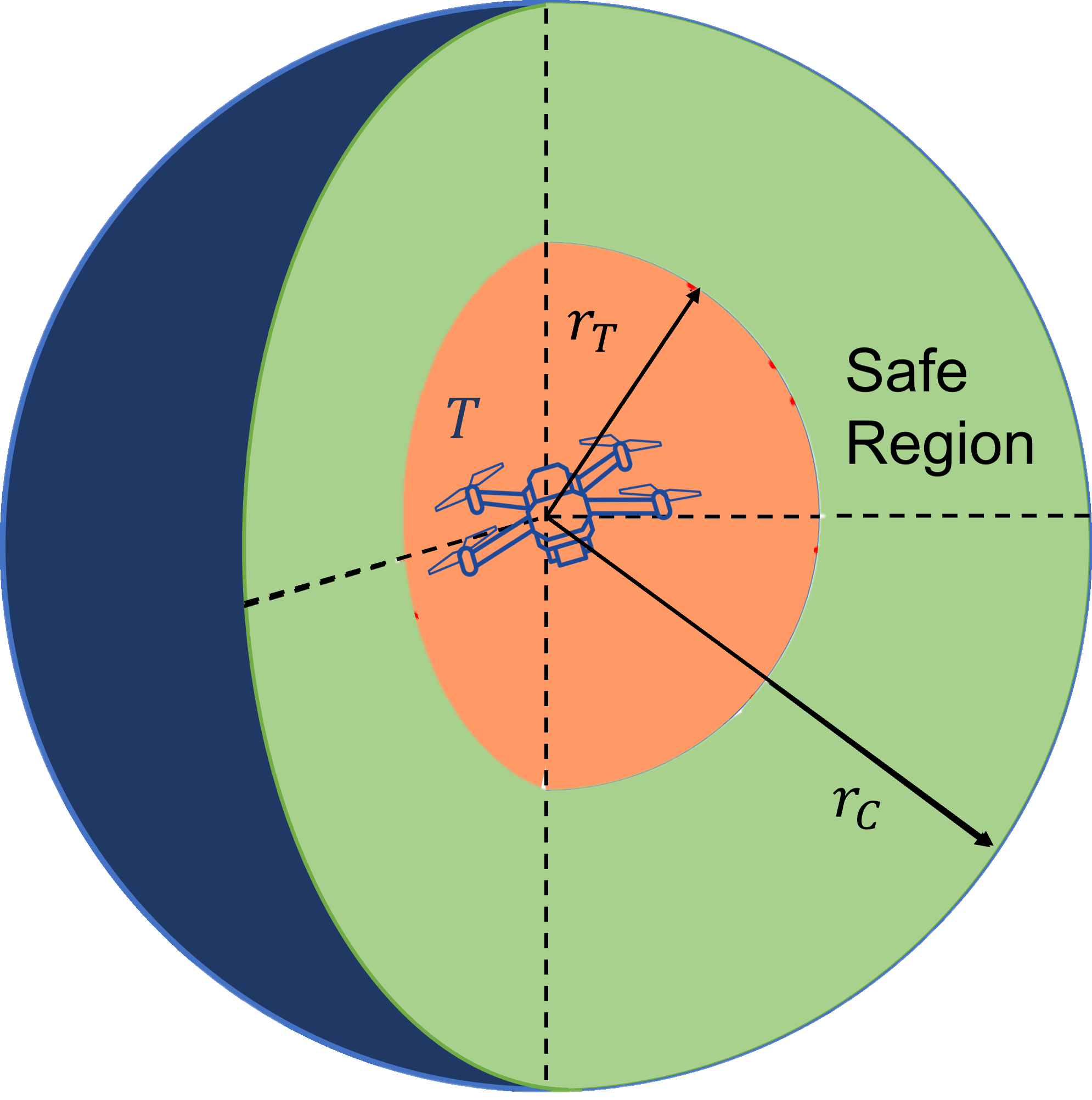
Figure 2: Pursuer’s regions of operation.

Let us denote the configuration or the position of the pursuer with respect to the target by $\phi(t)=[r(t),\theta(t),\psi(t)]^{\top}$. The safe region of operation, comprising of a spherical shell (or volume of cloud surrounding the target) of a fixed thickness ($r_{C}-r_{T}$), representing the allowable positions of the pursuer that ensures safety and enclosing is defined by the set $\Omega_{p}\coloneqq\left\{\left(r,\theta,\psi\right)\big{|}\,r\in\left[r_{T},r_{C}\right]\right\}.$ This set $\Omega_{p}$ remains constant in $F_{L}$ but varies with time in $F_{I}$ due to the mobility of the target. Consequently, $\phi(t)\in\Omega_{p}\;\forall\;t\geq 0$ is an additional critical objective to ensure that the pursuer remains in the predefined set of relative positions for all times. In 3D, achieving the second control objective will lead the pursuer to converge on a sphere of constant radius, maintaining the desired proximity to the target. This offers the pursuer numerous options for 3D orbits to effectively enclose the target. Moreover, incorporating the third control objective broadens these options, as the pursuer is now permitted to occupy a spherical shell representing the safe region. To summarize, the primary control objectives are to ensure (i) $\lim_{t\rightarrow\infty}V_{P}(t)\rightarrow V_{d}$, (ii) $\lim_{t\rightarrow\infty}r(t)\rightarrow r_{d}$, (iii) $\phi(t)\in\Omega_{p}\;\forall\;t\geq 0$. Additionally, we aim to minimize the pursuer’s overall control effort during enclosing by weighted effort allocation, thereby providing it even greater flexibility to shape its trajectory. In this letter, we aim to develop a generalized 3D guidance law for the pursuer to enclose an arbitrarily maneuvering target that guarantees the safety of the pursuer from the target while also ensuring maximal coverage during enclosing. The proposed guidance strategy enables the pursuer to maintain a fixed linear speed $V_{d}$ to lower the energy expenditure and converge to a set of relative positions $\Omega_{p}$. This inherently guarantees safety from the target’s movement and flexibility to occupy a larger set of positions relative to it. Further, we do not decouple the pursuer’s motion into separate channels, allowing it to maneuver freely in 3D, converging to any orbit situated surrounding the target within a volume of cloud (around $r_{d}$).

Before discussing the main results, we present an important result on the second-order Barrier Lyapunov Function relevant to control design with constraints on state variables. Such a function ensures stability with output constraints to guarantee the boundedness of the related error variable.

Lemma 1.

[28] Consider the open sets, $\mathcal{Z}_{1}\coloneqq\{z_{1}\in\mathbb{R},-a<z_{1}<b\}\subset\mathbb{R}$, $\mathcal{N}\coloneqq\mathbb{R}\times\mathcal{Z}_{1}\subset\mathbb{R}^{2}$ and the system $\dot{\eta}=h(t,\eta)$, where $\eta\coloneqq[w,z_{1}]^{\top}\in\mathcal{N}$ and $h$ is piecewise continuous in $t$ and locally Lipschitz in z, uniform in t, such that $h:\mathbb{R}_{>0}\times\mathcal{N}\rightarrow\mathbb{R}^{2}$. Suppose there exist two continuously differentiable and positive definite functions $U:\mathbb{R}\rightarrow\mathbb{R}_{\geq 0}$ and $V_{1}$, such that $V_{1}(z_{1})\rightarrow\infty,\;\text{as}\;\epsilon\rightarrow-a\;\text{or}\;\epsilon\rightarrow b$ and $\gamma_{1}\left(\lVert w\rVert\right)\leq U(\lVert w\rVert)\leq\gamma_{2}\left(\lVert w\rVert\right)$, where $\gamma_{1}$ and $\gamma_{2}$ are $K_{\infty}$ functions. Let $V_{2}(\eta)=V_{1}(z_{1})+U(w)$ and $\epsilon(0)$ belong to the set $\epsilon\in(-a,b)$. If the given inequality holds, $\dot{V}=\frac{\partial V}{\partial\eta}h\leq 0$, then $\epsilon(t)$ remains in the open set $\epsilon\in(-a,b),\;\forall\,t\in[0,\infty).$

III Main Results

In this section, we design the radial and lateral accelerations of the pursuer to satisfy the control objectives. We demonstrate that the proposed radial acceleration is independent of the lateral acceleration to simplify the design and lower the energy expenditure. This, in turn, will also aid in lowering the lateral acceleration effort because it may exhibit some dependence on the radial acceleration. This will be shown later.

We first design the pursuer’s radial acceleration to maintain the desired linear speed $V_{d}$, while enclosing the mobile target. To this end, we define the error as, $e_{v}=V_{P}-V_{d}$. On differentiating $e_{v}$ with respect to time and using (2c), we obtain the dynamics of this error variable as $\dot{e}_{v}=\dot{V}_{P}=a_{P}^{r}$, since $\dot{V}_{d}=0$. From this equation, it is evident that the linear speed error rate is directly related to the radial acceleration. Therefore, we propose the pursuer’s radial acceleration as

$$a_{P}^{r}=-K_{v}(V_{P}-V_{d}),$$ (3)

where $K_{v}>0$ denotes the controller gain.

Theorem 1.

Consider the equations of pursuer-target relative motion (1). The pursuer’s radial acceleration (3) allows it to maintain a constant speed throughout the engagement.

Proof.

Consider a Lyapunov Function candidate $V_{v}=\frac{1}{2}e_{v}^{2}$. On differentiating $V_{v}$ with respect to time and substituting for $\dot{e}_{v}$, we obtain, $\dot{V}_{v}=e_{v}\dot{e}_{v}=e_{v}a_{P}^{r}$. Choosing $a_{P}^{r}$ as in (3) renders the time derivative of the Lyapunov function candidate as $\dot{V}_{v}=-K_{v}e_{v}^{2}<0\,\forall\,e_{v}\in\mathbb{R}\setminus\{0\},$ if $K_{v}>0$. This implies that under the proposed control law, $V_{v}$ and hence $e_{v}$ decays to zero, resulting in the pursuer’s speed converging to the desired speed. On substituting the proposed control law $a_{P}^{r}$, we obtain the closed loop error dynamics as $\dot{e_{v}}=-K_{v}e_{v}$, which upon integration yields $e_{v}(t)=e_{v}(0)e^{-K_{v}t}$, thereby showing asymptotic convergence ($e_{v}\to 0$ as $t\to\infty$).∎

It follows from Theorem 1, the $V_{P}\to V_{d}$ as $t\to\infty$. In comparison to previous works, our approach simplifies the linear speed control design to lower the energy expenditure by requiring the pursuer to maintain a constant speed as opposed to dynamically changing $V_{P}$. Selecting $V_{d}$ such that $V_{d}>\sup_{t\geq 0}V_{T}$, provides an appropriate choice of $V_{d}$ that may provide the pursuer the capability to enclose the target at all times. In practice, such information can be easily obtained using onboard sensors or a ground station.

We now derive the lateral acceleration for the pursuer that allows it to converge to the desired proximity from the target while remaining in the safe region. We show that the proposed guidance law guarantees the global convergence of the range error with respect to the predefined state constraints. This implies that starting from all feasible initial configurations, the pursuer is able to achieve stable enclosing behavior without violating the safety constraints. Given the constant desired proximity $r_{d}$ of the pursuer from the target, we define the range error as $\epsilon(t)=r(t)-r_{d}$. Based on the safety constraint, the pursuer-target relative range $r$ is bounded between the predefined constraints in order to confine the movement of the pursuer within the safe region. Therefore, the error variable should also remain bounded as $-a<\epsilon<b$, where $a=r_{d}-r_{T}$ and $b=r_{C}-r_{d}$ denote the additional parameters representing the range error at boundaries. It is evident that different choices of $a$ and $b$ may lead to asymmetric bounds on the error variable. A larger value of $a$ will provide more flexibility to the pursuer to avoid collision with the target, while a smaller value of $b$ ensures that the pursuer does not maneuver far away from the desired proximity to ensure successful enclosing of the target at all times for maximal coverage. To analyze the behavior of range error, we differentiate $\epsilon$ with respect to time and use (1a) to obtain the dynamics of the error variable as, $\dot{\epsilon}=\dot{r}-\dot{r}_{d}=V_{T}\cos\gamma_{T}\cos\chi_{T}-V_{P}\cos\gamma_{P}\cos\chi_{P}$ since $\dot{r}_{d}=0$. It can be observed that the range error rate is directly related to the relative velocity along the pursuer-target LOS. On further differentiating $\dot{e}_{r}$ with respect to time and using (1) and (2), we obtain the dynamics of error rate as,

$$\ddot{\epsilon} =r\dot{\theta}^{2}+r\cos\theta^{2}\dot{\psi}^{2}+a_{P}^{r}\cos\gamma_{P}\cos\chi_{P}+\mathcal{U}+\Delta,$$ (4)

where we have separately clubbed the target’s and the pursuer’s control input-dependent terms. Here $\Delta=-a_{T}^{r}\cos\gamma_{T}\cos\chi_{T}-\sin\gamma_{T}\cos\chi_{T}a_{T}^{\gamma}-\sin\chi_{T}a_{T}^{\chi}$ denotes the target’s control input dependent term and $\mathcal{U}=\sin\gamma_{P}\cos\chi_{P}a_{P}^{\gamma}+\sin\chi_{P}a_{P}^{\chi}$ denotes the effective control input combining the pursuer’s lateral acceleration components. It can be observed from (4) that the range error dynamics has a relative degree of two with respect to the pursuer’s lateral acceleration components. Further, we will circumvent the need for exact information of the target’s control (that may be difficult to obtain in practice) by reasonably treating $\Delta$ as a bounded uncertainty. Note that various choices of $a_{P}^{\gamma}$ and $a_{P}^{\chi}$ may lead to the same $\mathcal{U}$. Therefore, we first propose the effective control input $\mathcal{U}$ to nullify the range error and its rate, given by

$$\mathcal{U} =-r\dot{\theta}^{2}-r\cos^{2}\theta\dot{\psi}^{2}-K_{v}\left(V_{p}-V_{d}\right)\cos\gamma_{P}\cos\chi_{P}$$

$$+\dot{\alpha}-{K}_{2}\mathrm{sign}{\left(\dot{r}-\alpha\right)}-\left[\frac{q}{a^{2}-\epsilon^{2}}+\frac{\left(1-q\right)}{b^{2}-\epsilon^{2}}\right]\epsilon,$$ (5)

where a sufficient condition on the controller gain $K_{2}$ is such that $K_{2}>|a_{\max}^{r}|+|a_{\max}^{\gamma}|+|a_{\max}^{\chi}|$ and $q\left(\epsilon\right)=\begin{cases}1,\;\text{if}\;\epsilon>0\\ 0,\;\text{if}\;\epsilon\leq 0\\ \end{cases}$ denotes a switching function with $\alpha$ denoting the stabilizing function given as,

$$\alpha =-\bigr{[}q(b^{2}-\epsilon^{2})+\left(1-q\right)(a^{2}-\epsilon^{2})\bigr{]}{K}_{1}\epsilon^{3},$$ (6)

where $K_{1}>0$ is also a controller gain. For brevity, we drop the argument of $q(\epsilon)$ from everywhere, and it will be understood that $q$ is a function of $\epsilon$.

Theorem 2.

Consider the equations of pursuer-target relative motion (1). The pursuer’s effective control effort (5) allows it to converge to the desired proximity around the target for maximal coverage during enclosing while also ensuring its safety.

Proof.

Consider an asymmetric Lyapunov Barrier Function candidate, $V_{1}(\epsilon)=q\log{\frac{b^{2}}{b^{2}-\epsilon^{2}}}+\left(1-q\right)\log{\frac{a^{2}}{a^{2}-\epsilon^{2}}}$, which is a convex combination of two barrier functions with only one of them activated at a particular instance of time, based on $q$. Let us assume a pseudo-variable $z=\dot{\epsilon}-\alpha$, where $\alpha$ is a stabilizing function to be designed. Differentiating $V_{1}$ with respect to time and using $\dot{\epsilon}=z+\alpha$, we obtain, $\dot{V}_{1}(\epsilon)=\Big{(}\frac{q}{b^{2}-\epsilon^{2}}+\frac{1-q}{a^{2}-\epsilon^{2}}\Big{)}\epsilon\left(z+\alpha\right).$ By selecting the the stabilizing function as in (6), it follows that $\dot{V}_{1}=-K_{1}\epsilon^{4}+\Big{(}\frac{q}{b^{2}-\epsilon^{2}}+\frac{1-q}{a^{2}-\epsilon^{2}}\Big{)}\epsilon z.$ Now let us consider a second Lyapunov function candidate, $V_{2}(z,\epsilon)=V_{1}+\frac{1}{2}z^{2},$ where the original Lyapunov candidate is augmented with $z$-dependent quadratic term. On differentiating $V_{2}$ with respect to time, we obtain $\dot{V}_{2}=-K_{1}\epsilon^{4}+\Bigr{[}\frac{q\epsilon}{b^{2}-\epsilon^{2}}+\frac{\left(1-q\right)\epsilon}{a^{2}-\epsilon^{2}}+r\dot{\theta}^{2}+r\cos\theta^{2}\dot{\psi}^{2}-K_{v}(V_{p}-V_{d})\cos\gamma_{P}\cos\chi_{P}+\mathcal{U}+\Delta-\dot{\alpha}\Bigr{]}z$ after using $\dot{z}=\ddot{\epsilon}-\dot{\alpha}$ and substituting for $\dot{V}_{1}$, $\ddot{\epsilon}$ and $a_{P}^{r}$. Choosing the effective control input as specified in (5) simplifies the preceding expression to, $\dot{V}_{2}=-K_{1}\epsilon^{4}+\left(-K_{2}\mathrm{sign}(z)+\Delta\right)z$, which consequently implies $\dot{V}_{2}\leq-K_{1}\epsilon^{4}-\left(K_{2}-|\Delta|\right)|z|$ and hence $\dot{V}_{2}\leq-\Big{(}K_{2}-\left(|a_{\max}^{r}|+|a_{\max}^{\gamma}|+|a_{\max}^{\chi}|\right)\Big{)}|z|-K_{1}\epsilon^{4}$, which reveals the sufficient condition provided after (5) to ensure that $\dot{V}_{2}<0\;\forall\;\{\epsilon,z\}\in\mathbb{R}^{2}\setminus\{0,0\}$. Therefore, $\epsilon\to 0$ and $z\to 0$ as $t\to\infty$. This results in the pursuer converging to the desired proximity around the target, that is, $r\to r_{d}$. It can be further deduced from Lemma 1, that $a<\epsilon(t)<b,\;\forall\;t>0$, provided that $a<\epsilon(0)<b$. ∎

From (6), one may observe that $\alpha\to 0$ as $\epsilon\to 0$. Therefore, from Theorem 2, we can also conclude that $\dot{r}\to 0$ as $t\to\infty$ since $z=\dot{r}-\alpha$. At steady-state, the pursuer converges to the desired proximity from the target, maintaining constant speed $V_{d}$, resulting in $\mathcal{U}\to-r_{d}\dot{\theta}^{2}-r_{d}\cos\theta^{2}\dot{\psi}^{2}$ from (5) denoting the centripetal acceleration required to maintain position on a sphere of radius $r_{d}$. Theorem 2 also provides guarantees on the boundedness of the range error, that is, $a<\epsilon<b$. This also implies $r_{T}<r(t)<r_{C}$ since $r_{d}$ is a constant. Thus, the pursuer consistently stays within the safe region surrounding the target, provided it starts within this region initially and eventually converges to the desired proximity. This essentially means that $\phi(t)\in\Omega_{p}\;\forall\;t\geq 0$ given $\phi(0)\in\Omega_{p}$, verifying the criticality of the safety condition as an additional control objective, thereby ensuring the pursuer avoids collision with the target at all times.

Although it might seem from (5) that the proposed effective control may potentially grow unbounded if $\epsilon=a$ or $\epsilon=b$. However, such a situation never arises as confirmed in Theorem 2 since the error variable always remains within the predefined constraints, never reaching the constraint boundaries. The first two terms in (5) represent the centripetal acceleration required to maintain a circular orbit at the current $r$ around the target. The third term in (5) represents the component of the radial acceleration along the LOS, indicating a relationship between the radial and lateral accelerations. The fifth and the sixth terms in (5) aid in adjusting the pursuer trajectory toward the desired proximity. Finally, the last two terms in (5) also ensure that the pursuer consistently stays within the safe region surrounding the target.

As previously mentioned, the effective control input $\mathcal{U}$ is a combination of the components of lateral acceleration in the pitch and yaw planes. This implies that infinite choices of $a_{p}^{\gamma}$ and $a_{p}^{\chi}$ can result in the same $\mathcal{U}$. Hence, we now formulate an optimization problem to distribute the control effort in the pitch and the yaw planes to achieve the effective lateral acceleration control $\mathcal{U}$ as proposed in (5). We define the cost function for optimization as $\mathcal{J}=\sqrt{\left(\frac{a_{P}^{\gamma}}{w_{1}}\right)^{2}+\left(\frac{a_{P}^{\chi}}{w_{2}}\right)^{2}}$, where $w_{1},w_{2}>0$ denote the weight parameters in the pitch and yaw channels, respectively. Such a cost function may represent the pursuer’s energy expenditure or maneuverability in terms of its acceleration in the pitch and yaw plane when $w_{1}=w_{2}$.

Theorem 3.

The optimal values of the pursuer’s lateral acceleration components in the pitch and yaw plane, $a_{P}^{\gamma}=\frac{\sin\gamma_{P}\cos\chi_{P}w_{1}^{2}\mathcal{U}}{(\sin\gamma_{P}\cos\chi_{P})^{2}w_{1}^{2}+(\sin\chi_{P})^{2}w_{2}^{2}}$ and $a_{P}^{\chi}=\frac{\sin\chi_{P}w_{2}^{2}\mathcal{U}}{(\sin\gamma_{P}\cos\chi_{P})^{2}w_{1}^{2}+(\sin\chi_{P})^{2}w_{2}^{2}}$ minimizes the cost function $\mathcal{J}$ under the constraints (5).

Proof.

For the proof of this theorem, we direct the reader to [6] and [22] for a detail explanation, which employs a similar technique for control (lateral acceleration) allocation.∎

It may seem that the acceleration components in Theorem 3 may grow unbounded if $(\sin\gamma_{P}\cos\chi_{P})^{2}w_{1}^{2}+(\sin\chi_{P})^{2}w_{2}^{2}=0$. However, this expression can become zero if and only if $\gamma_{p}=0$ and $\chi_{p}=0$. We show that such a scenario rarely arises and does not affect the target enclosing behavior. To analyze the dynamics of the pursuer’s angles, we define the pursuer’s effective lead angle $\sigma_{P}$ as the angle that the velocity vector subtends to the LOS and is given by the relationship, $\cos\sigma_{P}=\cos\gamma_{P}\cos\chi_{P}$. Thereby, we can infer that $\sigma_{P}\to 0$ if both $\gamma_{P}\to 0$ and $\chi_{P}\to 0$. Therefore, showing that $\sigma_{P}=0$ is not an equilibrium point is sufficient to show that the components in Theorem 3 do not grow unbounded. To this end, we differentiate the above-mentioned lead angle relationship with respect to time and use $a_{p}^{\gamma}$ and $a_{p}^{\chi}$ from Theorem 3 to obtain the dynamics of pursuer’s lead angle at the steady state when $\gamma_{p}=0$, $\chi_{P}=0$ since $\dot{\sigma}_{P}=\frac{-r_{d}\dot{\theta}^{2}-r_{d}\cos\theta^{2}\dot{\psi}^{2}}{\sin\sigma_{P}},$ where we have substituted $\epsilon\to 0$, $\dot{\epsilon}\to 0$, $\alpha\to 0$ and $\dot{\alpha}\to 0$. From this, it is evident that when $\sigma_{P}\to 0$, $\dot{\sigma}_{P}\to\infty$, which shows that $\sigma_{P}=0$ is not an equilibrium point. However, in the transient phase, $\sigma_{P}\to 0$ may occur momentarily and result in the saturation of lateral acceleration components (since the control inputs cannot be infinite in practice) that steers the pursuer away from $\sigma_{P}=0$ immediately. Hence, the proposed lateral acceleration components in Theorem 3 are non-singular almost everywhere. Furthermore, the proposed radial acceleration (3) and the optimal lateral acceleration components (as in Theorem 3) for the pursuer are dependent only on relative variables and independent of target control inputs, making our design robust to target’s maneuver and lucrative for the environment where global information is not readily available.

IV Simulation Results

We now demonstrate the efficacy of the proposed target enclosing guidance law by implementation on a high-fidelity quadrotor model via SITL simulations. We also compare this to the results obtained by simulating the nonlinear kinematic model (1) to demonstrate the robustness of our guidance law to unmodeled dynamics. In the nonlinear dynamical model, we utilize the equations of relative motion to represent the system dynamics without accounting for vehicle dynamics, autopilots, measurement noise, and computation latency. On the other hand, the SITL simulations replicate conditions closer to real-world scenarios, emulating a high-fidelity quadrotor model and incorporating various components (autopilot, ground station, companion computer) essential for autonomous flight. Our SITL setup employs Gazebo software to simulate a high-fidelity quadrotor model, Pixhawk autopilot, and MAVROS node of the Robot Operating System (ROS), connecting the vehicles to a companion computer [29]. Further, MATLAB is employed in the companion computer to receive vehicle information and issue the proposed guidance commands. Given our primary objective of developing the guidance law, we allow the pursuer access to the target’s global information. This facilitates the computation of requisite relative information for calculating the control inputs. Our simulation setup, operating on a 16 GB RAM AMD Ryzen 7 PC, achieves a sampling rate of 0.05 seconds (20Hz) for the guidance loop. Figure 3 depicts the flow of information between different components of the SITL setup.

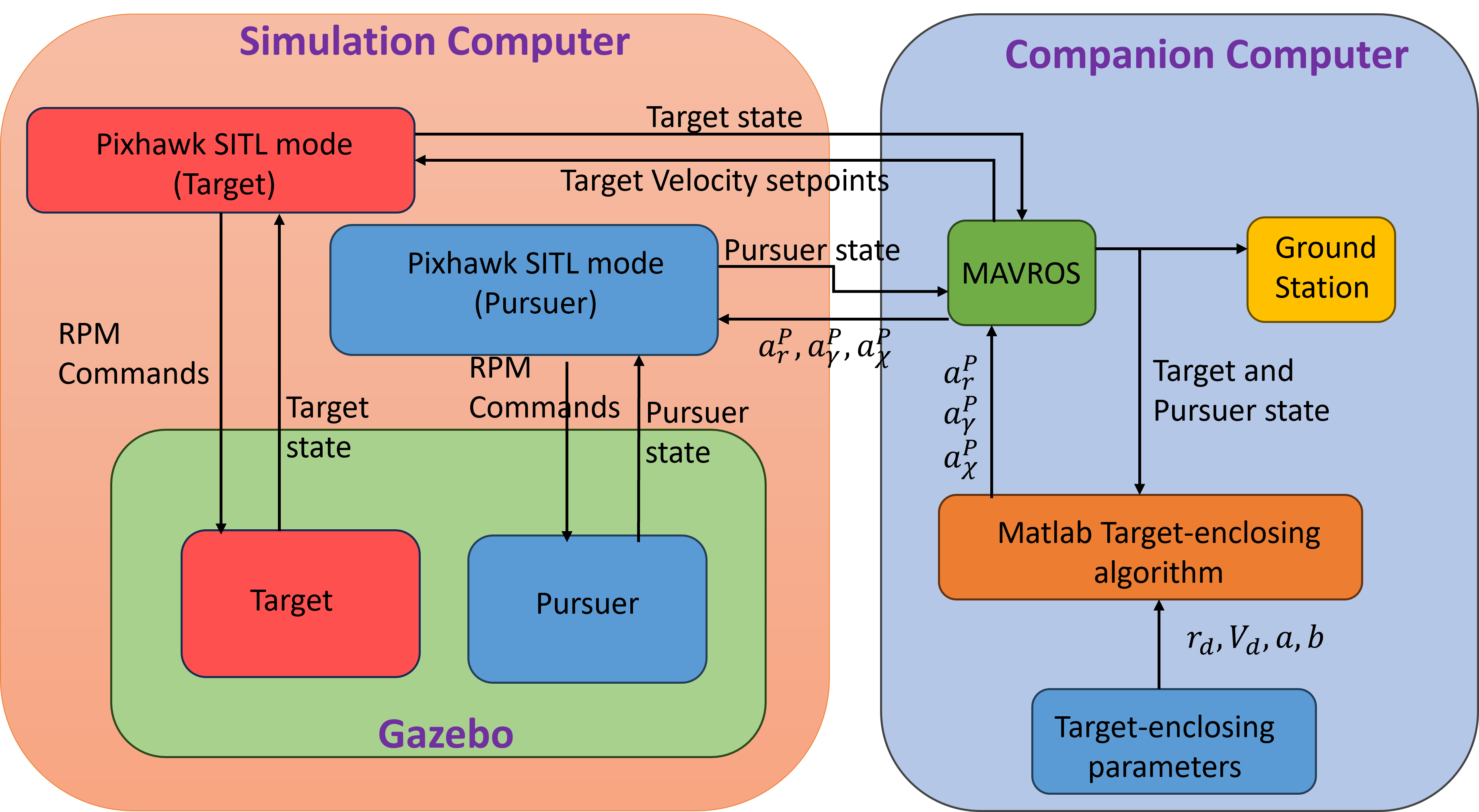
Figure 3: SITL Setup.

For all the experiments, the pursuer starts at $[x_{P},y_{P},z_{P}]^{\top}$ $=[0,0,15]^{\top}$ m, with $\gamma_{P}=10^{\circ}$ and $\chi_{P}=10^{\circ}$, while the target starts at $[x_{T},y_{T},z_{T}]^{\top}$ $=[12,12,15]^{\top}m$, with $\gamma_{T}=10^{\circ}$ and $\chi_{T}=10^{\circ}$, such that the initial values of relative variables are given as $r=18$ m, $\theta=0^{\circ}$ and $\psi=45^{\circ}$. The desired proximity from the target and the pursuer’s desired speed is selected as $r_{d}=8$ m and $V_{d}=5$ m/sec respectively, whereas the controller parameters and gains are chosen as $a=5$ m, $b=15$ m, $K_{1}=0.008$, $K_{2}=30$, $w_{1}=0.5$ and $w_{2}=0.5$. In the trajectory plots that follow, circular markers represent the initial position of the vehicles. Additionally, the videos of the vehicles’ trajectories for the simulations presented below can be found here.

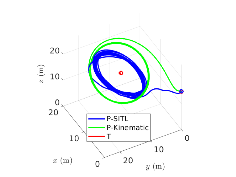
(a) ST.

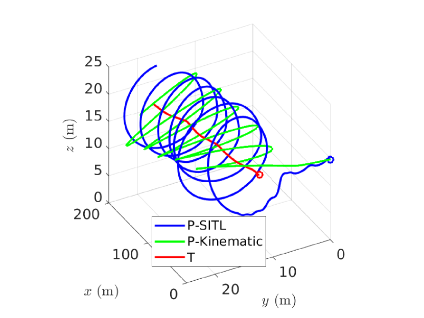
(b) CVT.

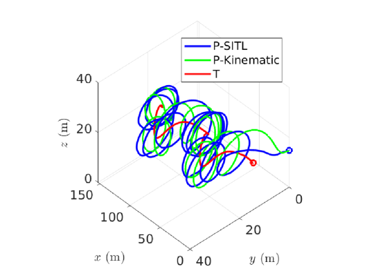
(c) MT.

Figure 4: Pursuer’s trajectories for various target maneuvers.

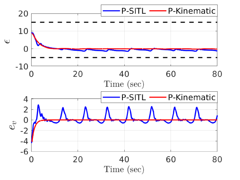
(a) ST.

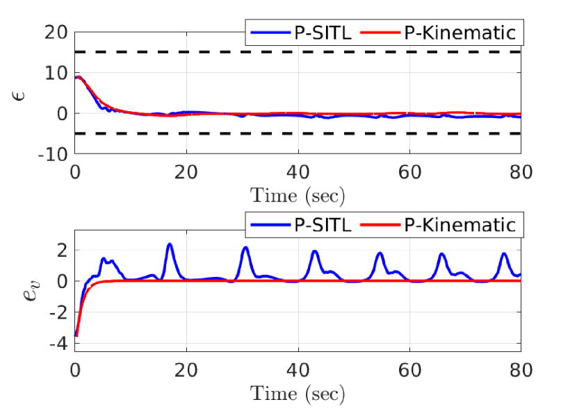
(b) CVT.

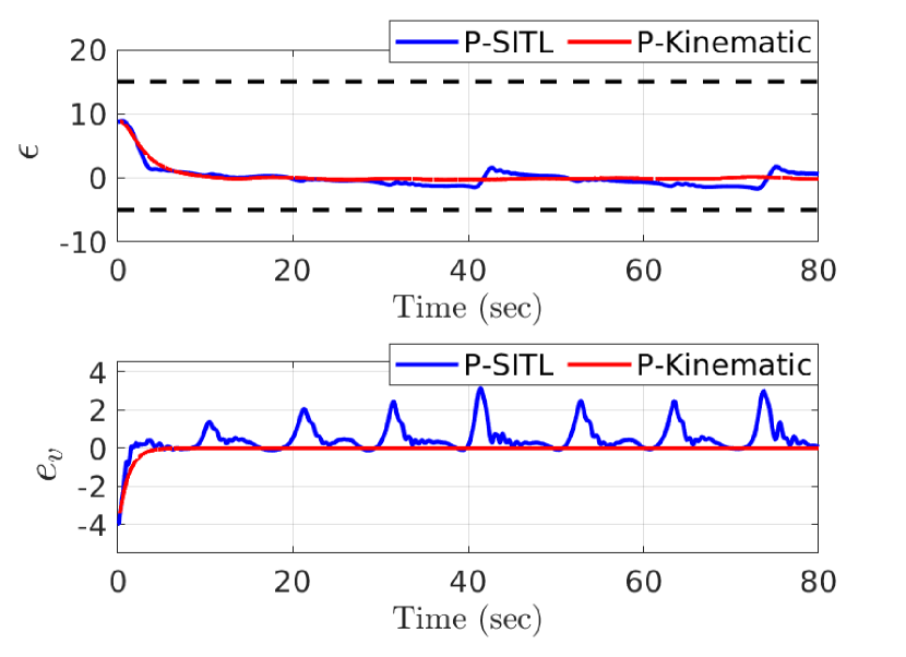
(c) MT.

Figure 5: Pursuer’s error variables for various target maneuvers.

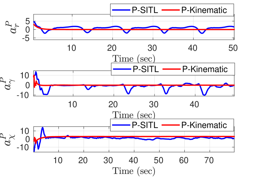
(a) ST.

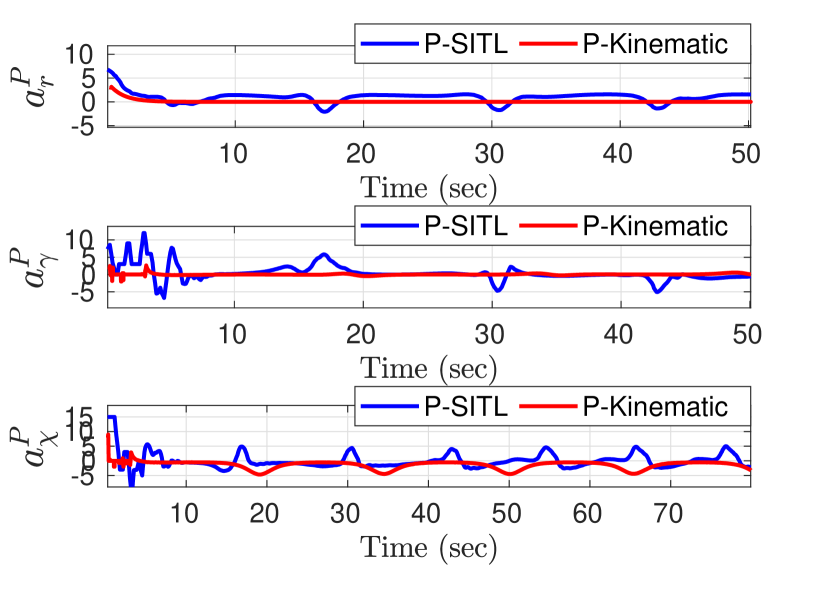
(b) CVT.

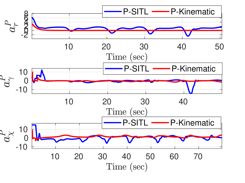
(c) MT.

Figure 6: Pursuer’s control inputs for various target maneuvers.

We present simulation results for three distinct target scenarios. In the first scenario, the target remains stationary (ST), while in the second scenario, the target moves in a straight line at a constant speed of $V_{T}=2$ m/s (CVT). Furthermore, in the third scenario, the target performs arbitrary maneuvers (MT), following a velocity profile described by $\mathbf{v_{T}}(t)=[\sin(10\pi t),\cos(10\pi t),0.5]^{\top}$ in the inertial frame of reference. Figure 4 illustrates the trajectories of the pursuer flexibly enclosing the target in arbitrary 3D orbits for different scenarios. However, the planes at which the pursuer converges to enclose the target are different for kinematic and SITL simulations, even when starting with the same conditions. This is due to the fact that the two simulation cases utilize different system dynamics, varying the conditions for target enclosing. Additionally, it is important to observe in Figure 4(a) that in the SITL simulations, the pursuer follows a set of enclosing trajectories, while in the kinematic simulation, the pursuer converges to a single orbit. This depicts the flexibility provided to the pursuer in our guidance approach, allowing it to converge to a region rather than a single orbit, even in practical scenarios. The profiles of the pursuer’s error variables are depicted in Figure 5. In the kinematic simulation, the range and speed errors quickly nullify and stabilize at zero. In SITL simulations, error profiles depict periodic deviation from zero, pertaining to the situation when the quadrotor moves from the highest to the lowest heights of the enclosing trajectory. This happens because of unmodeled dynamics. However, the range error remains within the desired bounds, ensuring the movement of the pursuer in the safe region and successful enclosing for all the target scenarios. The profiles of the pursuer’s control inputs are shown in Figure 6, where for the kinematic simulations, the profiles converge to the required steady-state values for target enclosing, whereas the SITL simulations show the periodic deviation from the steady-state values depicting high control demand due to momentary increase in the range and the speed errors. Despite such behaviors, the pursuer is able to enclose the target with maximal coverage while also adhering to the safety constraints, thereby exhibiting a certain degree of robustness during implementation.

V Conclusions

We proposed a 3D guidance law for the pursuer to enclose a mobile target where the pursuer is constrained to maneuver only within the safe region of operation. The pursuer’s radial acceleration is designed to achieve the desired speed, while the lateral accelerations are designed to steer the pursuer on enclosing shapes around the target. Our design provides guarantees on the boundedness of the pursuer-target relative range between the predefined bounds, preventing pursuer-target collision and ensuring the pursuer’s capability to enclose the target at all times with maximal coverage. We utilized coupled engagement kinematics and allocated control effort via static energy minimization, resulting in generalized 3D safe target enclosing behavior for the pursuer, which only requires information on relative variables. Although our design does not account for aerodynamic parameter variation or external/measurement disturbances, implementation of the guidance law on a quadrotor UAV in SITL simulations depicted the robustness of our approach to target maneuver, vehicle dynamics, and autopilot dynamics in achieving stable enclosing behavior. Extension to multiagent settings, design with full dynamics-based vehicle modeling, and including additional constraints such as obstacles could be interesting future directions to pursue.

References

- [1] J. Scherer and B. Rinner, “Multi-uav surveillance with minimum information idleness and latency constraints,” IEEE Robotics and Automation Letters, vol. 5, no. 3, pp. 4812–4819, 2020.
- [2] X. Lin, Y. Yazıcıoğlu, and D. Aksaray, “Robust planning for persistent surveillance with energy-constrained uavs and mobile charging stations,” IEEE Robotics and Automation Letters, vol. 7, no. 2, pp. 4157–4164, 2022.
- [3] N. Chebrolu, T. Läbe, and C. Stachniss, “Robust long-term registration of uav images of crop fields for precision agriculture,” IEEE Robotics and Automation Letters, vol. 3, no. 4, pp. 3097–3104, 2018.
- [4] M. Silic and K. Mohseni, “Field deployment of a plume monitoring uav flock,” IEEE Robotics and Automation Letters, vol. 4, no. 2, pp. 769–775, 2019.
- [5] P. Kumar Ranjan, A. Sinha, Y. Cao, D. Tran, D. Casbeer, and I. Weintraub, “Energy-efficient ring formation control with constrained inputs,” Journal of Guidance, Control, and Dynamics, vol. 46, no. 7, pp. 1397–1407, 2023.
- [6] A. Sinha and Y. Cao, “Three-dimensional autonomous guidance for enclosing a stationary target within arbitrary smooth geometrical shapes,” IEEE Transactions on Aerospace and Electronic Systems, vol. 59, no. 6, pp. 9247–9256, 2023.
- [7] T.-H. Kim and T. Sugie, “Cooperative control for target-capturing task based on a cyclic pursuit strategy,” Automatica, vol. 43, no. 8, pp. 1426–1431, 2007.
- [8] “Pursuit formations of unicycles,” Automatica, vol. 42, no. 1, pp. 3–12, 2006.
- [9] E. W. Frew, D. A. Lawrence, and S. Morris, “Coordinated standoff tracking of moving targets using lyapunov guidance vector fields,” Journal of Guidance, Control, and Dynamics, vol. 31, no. 2, pp. 290–306, 2008.
- [10] Y. Gao, C. Bai, L. Zhang, and Q. Quan, “Multi-uav cooperative target encirclement within an annular virtual tube,” Aerospace Science and Technology, vol. 128, p. 107800, 2022.
- [11] A. A. Pothen and A. Ratnoo, “Curvature-constrained lyapunov vector field for standoff target tracking,” Journal of Guidance, Control, and Dynamics, vol. 40, no. 10, pp. 2729–2736, 2017.
- [12] S. Lim, Y. Kim, D. Lee, and H. Bang, “Standoff target tracking using a vector field for multiple unmanned aircrafts,” Journal of Intelligent & Robotic Systems, vol. 69, pp. 347–360, 01 2013. Copyright - Springer Science+Business Media Dordrecht 2013; Last updated - 2014-08-23.
- [13] D. Zhang, H. Duan, and Z. Zeng, “Leader–follower interactive potential for target enclosing of perception-limited uav groups,” IEEE Systems Journal, vol. 16, no. 1, pp. 856–867, 2022.
- [14] S. Park, “Circling over a target with relative side bearing,” Journal of Guidance, Control, and Dynamics, vol. 39, no. 6, pp. 1454–1458, 2016.
- [15] Y. Cao, “Uav circumnavigating an unknown target under a gps-denied environment with range-only measurements,” Automatica, vol. 55, pp. 150–158, 2015.
- [16] S. Park, “Guidance law for standoff tracking of a moving object,” Journal of Guidance, Control, and Dynamics, vol. 40, no. 11, pp. 2948–2955, 2017.
- [17] M. Deghat, I. Shames, B. D. O. Anderson, and C. Yu, “Localization and circumnavigation of a slowly moving target using bearing measurements,” IEEE Transactions on Automatic Control, vol. 59, no. 8, pp. 2182–2188, 2014.
- [18] Y. Lan, G. Yan, and Z. Lin, “Distributed control of cooperative target enclosing based on reachability and invariance analysis,” Systems & Control Letters, vol. 59, no. 7, pp. 381–389, 2010.
- [19] P. Jain, C. K. Peterson, and R. W. Beard, “Encirclement of moving targets using noisy range and bearing measurements,” Journal of Guidance, Control, and Dynamics, vol. 45, no. 8, pp. 1399–1414, 2022.
- [20] A. Sinha and Y. Cao, “Nonlinear guidance law for target enclosing with arbitrary smooth shapes,” Journal of Guidance, Control, and Dynamics, vol. 45, no. 11, pp. 2182–2192, 2022.
- [21] A. Sinha and Y. Cao, “3-d nonlinear guidance law for target circumnavigation,” IEEE Control Systems Letters, vol. 7, pp. 655–660, 2023.
- [22] A. Sinha and Y. Cao, “Three-dimensional guidance law for target enclosing within arbitrary smooth shapes,” Journal of Guidance, Control, and Dynamics, vol. 46, no. 11, pp. 2224–2234, 2023.
- [23] P. K. Ranjan, A. Sinha, and Y. Cao, “Self-organizing multiagent target enclosing under limited information and safety guarantees,” 2024.
- [24] P. K. Ranjan, A. Sinha, and Y. Cao, “Robust uav guidance law for safe target circumnavigation with limited information and autopilot lag considerations,” AIAA SCITECH 2024 Forum, 2024.
- [25] H. Oh, S. Kim, H.-s. Shin, B. A. White, A. Tsourdos, and C. A. Rabbath, “Rendezvous and standoff target tracking guidance using differential geometry,” Journal of Intelligent & Robotic Systems, vol. 69, pp. 389–405, 01 2013. Copyright - Springer Science+Business Media Dordrecht 2013; Last updated - 2014-08-23.
- [26] H. Li, Y. Cai, J. Hong, P. Xu, H. Cheng, X. Zhu, B. Hu, Z. Hao, and Z. Fan, “Vg-swarm: A vision-based gene regulation network for uavs swarm behavior emergence,” IEEE Robotics and Automation Letters, vol. 8, no. 3, pp. 1175–1182, 2023.
- [27] E. Price, M. J. Black, and A. Ahmad, “Viewpoint-driven formation control of airships for cooperative target tracking,” IEEE Robotics and Automation Letters, vol. 8, no. 6, pp. 3653–3660, 2023.
- [28] K. P. Tee, S. S. Ge, and E. H. Tay, “Barrier lyapunov functions for the control of output-constrained nonlinear systems,” Automatica, vol. 45, no. 4, pp. 918–927, 2009.
- [29] Pixhawk Autopilot, ”Multi-Vehicle Simulation with Gazebo Classic”, https://docs.px4.io/main/en/sim_gazebo_classic/multi_vehicle_simulation.html (Accessed: 12-14-2023).