Measurement of Interstellar Magnetization by Synchrotron Polarization Variance
Abstract
Since synchrotron polarization fluctuations are related to the fundamental properties of the magnetic field, we propose the polarization intensity variance to measure the Galactic interstellar medium (ISM) magnetization. We confirm the method’s applicability by comparing it with the polarization angle dispersion and its reliability by measuring the underlying Alfvénic Mach number of MHD turbulence. With the finding of the power-law relation of between polarization intensity variance and Alfvénic Mach number , we apply the new technique to the Canadian Galactic Plane Survey (CGPS) data, achieving Alfvénic Mach number of the Galactic ISM. Our results show that the low-latitude Galactic ISM is dominated by sub-Alfénic turbulence, with approximately between 0.5 and 1.0.
1 Introduction
It is generally accepted that interstellar medium (ISM) is turbulent and magnetized, and is ubiquitous in the universe (Armstrong et al. 1995; Elmegreen & Scalo 2004). Magnetohydrodynamic (MHD) turbulence plays a crucial role in many key astrophysical processes, such as star formation, cosmic ray acceleration and propagation, as well as magnetic reconnection (e.g., Larson 1981; Lazarian & Vishniac 1999; Schlickeiser 2003; McKee & Ostriker 2007; Lazarian et al. 2015). Determining the properties of magnetized turbulence is a crucial step in exploring astrophysical activity. However, the measurement of ISM magnetic field strength is extremely challenging.
At present, several techniques measuring magnetic field strength have been proposed. As is well known, the Zeeman effect caused by spectral line splitting is a classic method in measuring the magnetic field component along the line of sight (LOS), requiring high instrument sensitivity and a longer observational integration time (Goodman et al. 1989; Crutcher 1999; Bourke et al. 2001; Crutcher et al. 2010; Mao et al. 2021; Inoue 2023). The traditional Faraday rotation synthesis can well present the magnetic structure of the Milky Way and nearby galaxies. However, this method cannot determine the magnetic field direction due to the ambiguity of the phase angle (Burn 1966; Beck & Wielebinski 2013). The Davis-Chandrasekhar-Fermi (DCF, Davis 1951; Chandrasekhar & Fermi 1953) method utilizes fluctuations in observed polarization and gas Doppler shift velocity to estimate the projected magnetic field strength by , where is an adjustable factor (typically ), is the LOS velocity dispersion, and is polarization angle dispersion. In general, this method results in the measured magnetic field strength deviating from the expected value. Note that this method is based on the assumption of incompressible isotropic turbulence. In fact, the theoretical and observational results imply that ISM turbulence is compressible and anisotropic (Goldreich & Sridhar 1995, henceforth GS95; Cho & Lazarian 2002; Spangler & Spitler 2004).
Recently, different improved versions of the DCF method have been enhanced. For instance, Lazarian et al. (2022) proposed a differential measure approach where the adjustable factor in the DCF method is related to turbulence properties rather than a constant. In the framework of the DCF method, different effects have been included into the DCF method such as the average effect of independent eddies in the LOS direction (Cho & Yoo 2016), atomic arrangement effect (Pavaskar et al. 2023), and polarization angle difference as a function of the distance between a pair of measurement points (Falceta-Gonçalves et al. 2008; Hildebrand et al. 2009; Houde et al. 2009). For the latter, due to the angle dispersion function affected by the integration effect along the LOS, the spatial range to measure should be limited within scales smaller than (Cho & Yoo 2016; Liu et al. 2021).
With the modern understanding of the MHD turbulence theory, other techniques for measuring the strength of magnetic fields have been proposed. First, the anisotropy of the structure functions has been proposed considering the velocity channel (Esquivel & Lazarian 2011; Esquivel et al. 2015), and the velocity centroid and rotation measurement (Xu & Hu 2021; Hu et al. 2021). Second, gradient measurements involve velocity (Lazarian et al. 2018) and synchrotron polarization (Carmo et al. 2020). Third, the ratio of the E and B modes arises from dust polarization (Cho 2023).
In the earlier numerical work, Zhang et al. (2016) proposed the synchrotron polarization dispersion for measuring the scaling index of underlying MHD turbulence (see also Lazarian & Pogosyan 2016 for theoretical predictions). This method is named polarization frequency analysis (PFA) which considers the variance of polarization intensity as a function of the square of wavelength . They found that the turbulent spectral index can be successfully recovered from the polarization intensity variance in the region dominated by the mean field. In this work, we want to know whether polarization intensity variance can be used as a complementary method for measuring magnetic field strength. At the same time, to enhance the reliability of our techniques, we will also explore the use of polarization angle dispersion to measure magnetization levels.111When mentioning the magnetization or magnetization levels in this paper, we specifically refer to it as the Alfvénic Mach number .
The structure of this paper is regularized as follows. In Section 2, we provide theoretical fundamentals including the properties of MHD turbulence, synchrotron polarization radiation, and statistical measure techniques. Section 3 describes simulation methods with basic parameter setup. Numerical results and application of observational data are presented in Sections 4 and 5, respectively. Sections 6 and 7 give discussion and summary, respectively.
2 Theoretical Considerations
2.1 Modern understanding of MHD Turbulence
The modern understanding of the MHD turbulence theory can be traced back to the work of GS95, which focused on incompressible and trans-Alfvénic (with Alfvénic Mach number ) turbulence and predicted the scale-dependent anisotropy expressed as , where and are the scales parallel and perpendicular to the local magnetic fields, respectively. Essentially, the turbulent cascade in the perpendicular direction and wave-like motion in the parallel direction are mutually coupled, establishing a critical balance condition by
| (1) |
between turbulent eddy turnover time and the Alfvén wave period. Here, is the Alfvénic velocity related to the magnetic field of and gas density of . With this critical balance assumption, GS95 found that the cascading rate remains constant, i.e., , which results in the classical Kolmogorov’s spectrum of (Kolmogorov 1941).
In later studies, GS95’s work, in relation to trans-Alfvénic turbulence, was generalized to two scenarios: and (Lazarian & Vishniac 1999; Lazarian 2006), where is the injection velocity at the injection or outer scale . For the former, , Lazarian & Vishniac (1999) found a transition scale
| (2) |
In the range of , with remaining unchanged while continuously decreasing until reaching the critical equilibrium condition at the scale , the turbulent cascade presents the weak turbulence properties. In the range of , where is the turbulent dissipation scale222In general, at the scale smaller than , turbulence dissipation is dominated by numerical dissipation ( cells, Hernández-Padilla et al. 2020). If the transition scale is smaller than the dissipation scale, the numerical results connecting with the astrophysical environment may cause problems (Brandenburg & Lazarian 2013)., turbulence cascade shows the strong turbulence properties, with the parallel and perpendicular scale relationship of
| (3) |
and with velocity and scale relationship
| (4) |
Note that when , Eqs. (3) and (4) will return to the original GS95 relationship of and , respectively.
For the latter, , Lazarian (2006) predicted that this super-Alfvénic turbulence has the transition scale of
| (5) |
where the anisotropy of turbulent eddies occurs. When , the magnetic field is not dynamically important at the maximum scale, and within the scale range of , turbulence follows an anisotropic Kolmogorov cascade (see Lazarian (2006) for more details).
2.2 Synchrotron Polarization
When relativistic electrons move in a ubiquitous magnetic field, the synchrotron radiation process inevitably arises. With an assumption of a uniformly isotropic power-law energy distribution for relativistic electrons, where is the electron energy and is the photon spectral index related to the electron spectral index by the relation of , we have the synchrotron intensity per unit frequency interval (Ginzburg & Syrovatskii 1965)
| (6) |
where represents the integration length along the LOS. Based on Eq.(6), we can get the linearly polarized intensity by
| (7) |
The Stokes parameters and are related to the polarization intensity by , , where is the polarization angle. Defining the complex polarization vector
| (8) |
we can write the polarization intensity as
| (9) |
Furthermore, when synchrotron radiation experiences a radiative transfer, the Faraday rotation effect will result in the depolarization of the radiation signal. The resulting polarization angle can be re-written as
| (10) |
where the rotation measure (RM) is given by
| (11) |
Here, in units of is the thermal electron density, in units of is the parallel component of the magnetic field along the LOS, and in units of is the path length.
2.3 Statistical Measure Techniques
Since magnetic field fluctuations cause a change in polarization signal, the properties of the magnetic field can be explored through analyzing the polarization observational information. According to Zhang et al. (2016), we define the correlation function of the polarization intensity as
| (12) |
where and denote the spatial locations on the plane of the sky. Considering the correlation of polarization intensities at the same spatial separation =0 on the plane of the sky, we name it as the polarization variance, i.e., one-point statistics. Practically, we normalize the polarization intensity variance in units of the mean of the polarization intensity. This procedure can eliminate the influence of dimensionality on the statistics for realistic observations in different astrophysical environments. Moreover, according to the analysis of the DCF method (e.g., Lazarian et al. 2022), we define the polarization angle dispersion by
| (13) |
With the above two definitions (Eqs. (12) and (13)), this paper will explore how and connect with the magnetization by the Bayesian analysis method. To implement Bayesian statistics and fitting algorithms, we use the Python package PyMC to solve general Bayesian statistical inference and prediction problems (Patil et al. 2010). With the PyMC, we can determine the best fitting level and fitting error from two variables. From a theoretical view, with fundamental parameter assumptions such as the parameter depending on the observable , a linearly fitted parameter model , and a normal distribution error , we have the linear regression relationship of . Therefore, this model can be represented as a probability distribution , where denotes a normally distributed random variable, a mean of linear predictor and a square variance of .
In practice, we consider the measured quantity as the independent variable for linear fitting, and direct statistical quantities ( and ) as the dependent variables. The assumed distributions and parameters of all priors in this linear model are listed as follows
| (14) |
| (15) |
| (16) |
We use Markov Chain Monte Carlo methods in Bayesian analysis, after choosing posterior 333We have tested the influence of sample numbers on the results. When choosing posterior samples are greater than , the numerical results will remain the same., with each sample including parallel chains for tune, the output with the highest density interval can provide the mean, standard deviation, and intercept of the linear fitting slope.
3 Generation of MHD Turbulence Simulation Data
To simulate magnetized turbulent ISM, we consider a set of governing equations of MHD turbulence as follows:
| (17) |
| (18) |
| (19) |
| (20) |
where is gas density, the evolution time of the fluid, gas pressure, the current density, and a random driving force. At the same time, we use the isothermal state equation to close the above equations.
When numerically solving the above equations, we use a single-fluid, operator-split, and staggered-grid MHD Eulerian code ZEUS-MP/3D (Hayes et al. 2006). We set a non-zero uniform magnetic field along the -axis, resulting in a total magnetic field , where is a fluctuating magnetic field, and an average density . With the periodic boundary conditions and solenoid turbulence driving, we run two sets of simulations with different resolutions: Group with a numerical resolution of 792 at a driving wavenumber of , and Group with the resolution of 480 at , by changing the uniform magnetic field and injection energy. When reaching a quasi-steady state at ( being Alfvénic timescale), we terminate the simulation and then output the information of the last snapshot, which includes the 3D velocities, magnetic fields, and density. Using the definitions of Alfvénic Mach number , sonic Mach number of , and the plasma parameter , we characterize different data groups as listed in Table 1. The latter, , describes the compressibility of turbulence, with a low corresponding to the compressible regime dominated by magnetic pressure, and a high to the nearly incompressible one dominated by gas pressure.
| Models | A1 | A2 | A3 | A4 | A5 | A6 | A7 | A8 | A9 | A10 | B1 | B2 | B3 | B4 | B5 | B6 | B7 | B8 | B9 |
|---|---|---|---|---|---|---|---|---|---|---|---|---|---|---|---|---|---|---|---|
| 0.64 | 1.17 | 0.61 | 0.82 | 1.01 | 1.19 | 1.38 | 1.55 | 1.67 | 1.71 | 0.83 | 2.22 | 0.32 | 0.59 | 0.48 | 0.94 | 0.49 | 1.02 | 0.52 | |
| 0.63 | 0.60 | 5.81 | 5.66 | 5.62 | 5.63 | 5.70 | 5.56 | 5.50 | 5.39 | 0.25 | 0.24 | 0.98 | 1.92 | 0.48 | 0.93 | 0.16 | 0.34 | 0.05 | |
| 2.06 | 7.61 | 0.02 | 0.04 | 0.07 | 0.09 | 0.12 | 0.16 | 0.18 | 0.20 | 22.74 | 172.02 | 0.21 | 0.19 | 2.02 | 2.09 | 18.99 | 17.52 | 206.56 | |
| 0.1 | 0.03 | 4.6 | 2.6 | 1.7 | 1.1 | 0.8 | 0.6 | 0.5 | 0.4 | 0.01 | 0.001 | 1.0 | 1.0 | 0.1 | 0.1 | 0.01 | 0.01 | 0.001 | |
| 0.50 | 0.86 | 0.47 | 0.63 | 0.76 | 0.87 | 1.02 | 1.12 | 1.25 | 1.39 | 0.64 | 1.84 | 0.23 | 0.46 | 0.39 | 0.74 | 0.40 | 0.80 | 0.39 |
4 Results
4.1 Images of polarization intensity and polarization angle with Faraday rotation
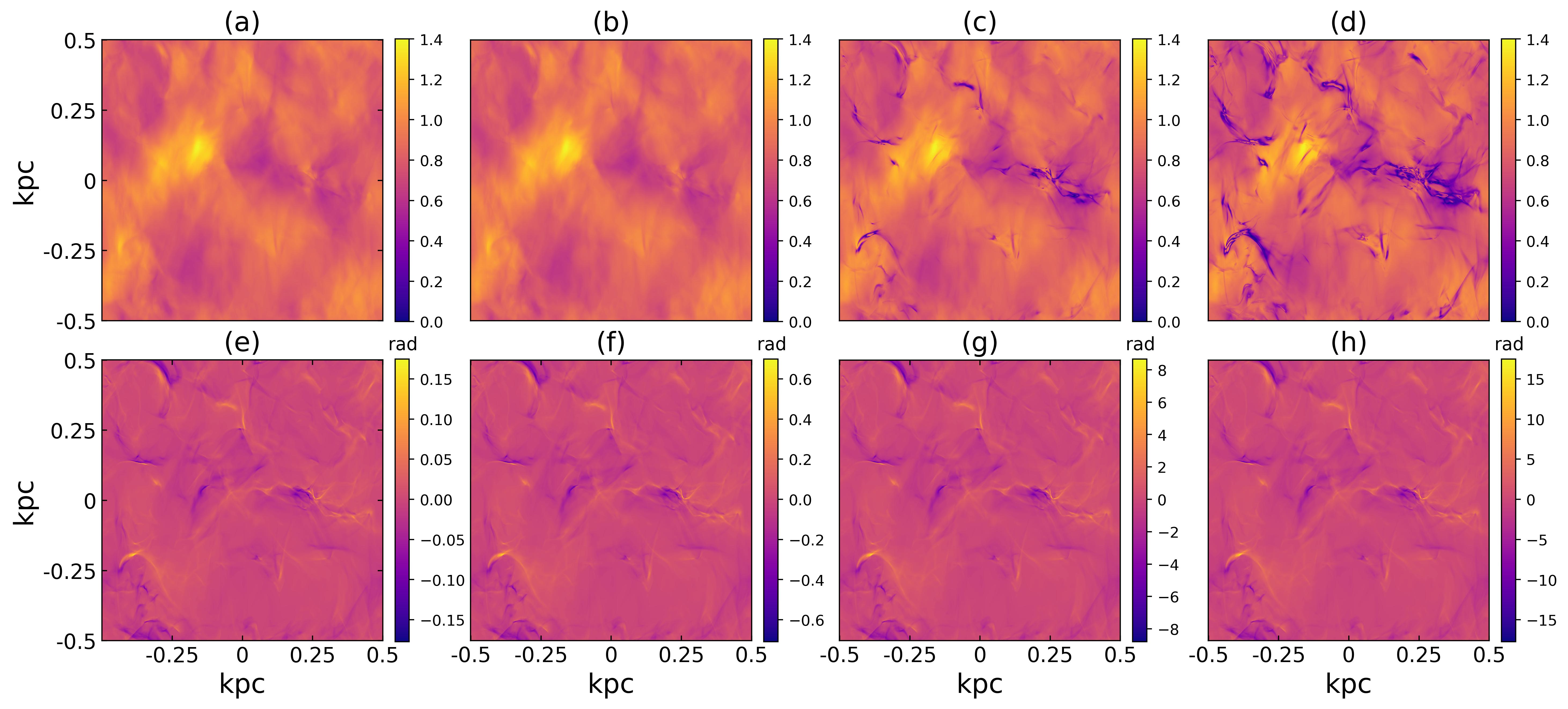
To generate synchrotron polarization observations, we use typical parameters from the Galactic ISM, such as thermal electron number density of , spectral index of relativistic electron of (note that change in the index cannot affect our results; see Zhang et al. (2018) for more details), magnetic field strength of , Faraday integral depth of . Furthermore, we consider the -axis along the LOS direction, which results in the plane of the sky parallel to the - plane. Based on Section 2.2, we obtain the images of the Stokes parameters , , and using the above parameters.
As is well known, when a linearly polarized electromagnetic wave propagates along a magnetic field, the polarization direction will change due to the influence of Faraday rotation. Equation (10) indicates that the change in polarization angle is wavelength-dependent. To understand the effect of Faraday rotation on polarization radiation, we present the polarization intensity (upper row) and polarization angle (lower row) maps at different frequencies in Figure 1. From left to right, images correspond to the frequencies of 10, 5, 1.42, and , respectively. As shown in the upper panels of Figure 1, with decreasing frequency, the maximum value of polarization intensity is slightly lower, while the minimum value is significantly lower. At the low-frequency regime (see panel (d)), we can see significantly elongated filament structures due to the enhancement of Faraday depolarization.
The lower panels of Figure 1 present the distribution of polarization angle. At the high frequency of (see panel (e)), it is , where the Faraday rotation effect is almost negligible. As the frequency decreases, we see that Faraday rotation increases the polarization angle. When reduced to 1.42 , polarization angle rotates about (see panel (g)).
4.2 Finding of the power-law relationship
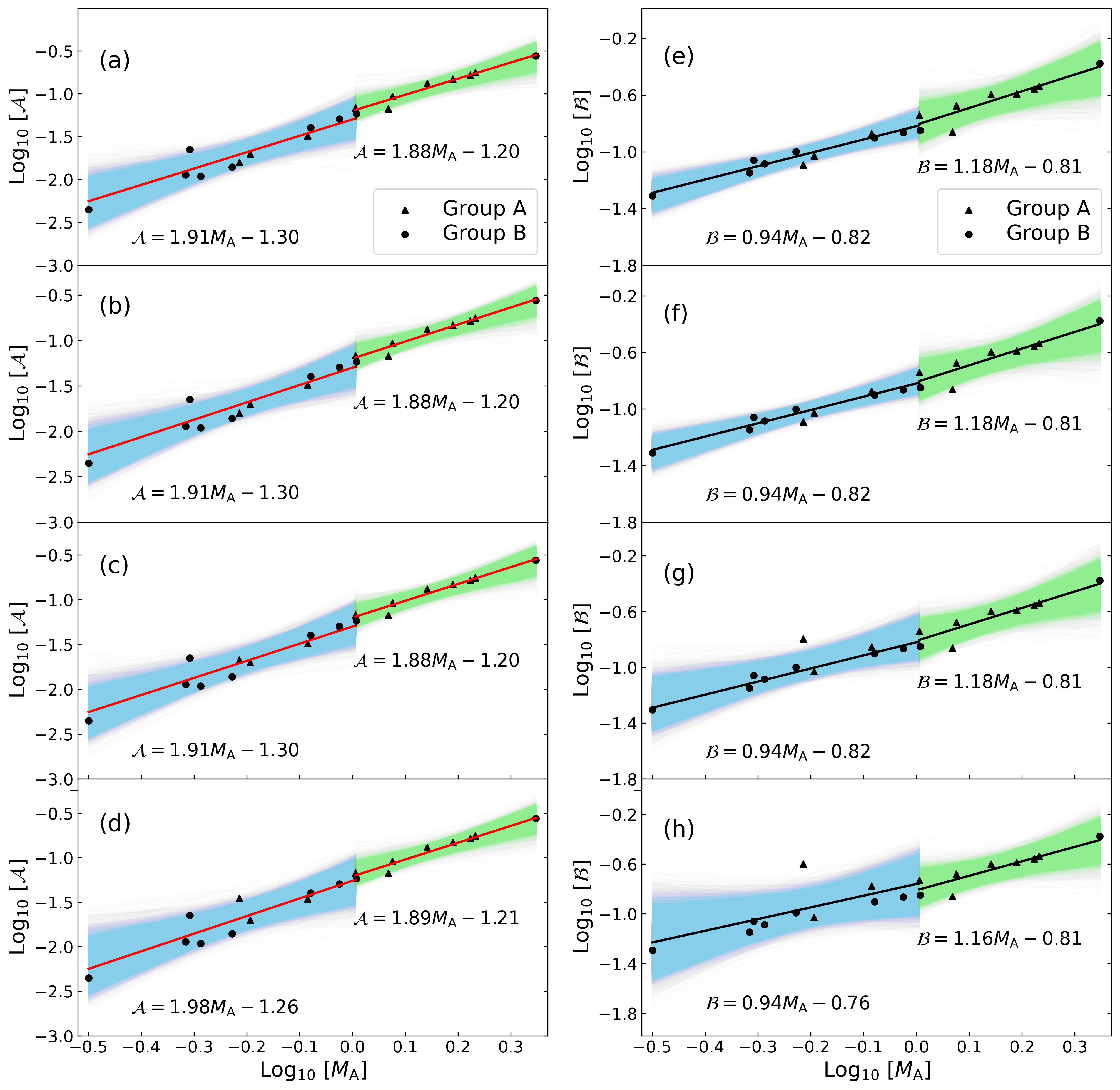
Based on Sections 2.3 and 4.1, we analyze the polarization intensity variance and polarization angle dispersion using each MHD turbulence data listed in Table 1. Then, we use Bayesian analysis to search for the power-law relationship of and as a function of . Given the differences in the turbulence nature of MHD (see Section 2.1), we perform a separate fitting for the sub- and super-Alfvénic regimes.
The results are plotted in Figure 2 for vs. (left column) and vs. (right column). From top to bottom, the frequencies used are 10, 5, 1.42, and , respectively. The blue and green shaded areas represent the highest density interval , i.e., the fitted confidence level, in the sub- and super-Alfvénic regimes, respectively. In the sub-Alfvénic regime, we find the power-law relations of and , while in the super-Alfvénic regime, we obtain the relations of and . These relationships have been transformed from a logarithmic space to a linear space. In the range from 10 to , we find that the power-law relation remains the same, except for the change in fitting error as summarized in Table 2 due to the Faraday rotation effect. Although the power-law relationship between and changes slightly when the frequency decreases to , we focus more on the results at a frequency of , so this has no impact on our observational application in Section 5.
As a result, since the polarization intensity variance and polarization angle dispersion exhibit a good power-law relationship with , we can employ these relations to determine the magnetization of the ISM.
| Methods | Frequencies | Sub-Alfvénic | Super-Alfvénic |
|---|---|---|---|
4.3 Testing for the measurement techniques
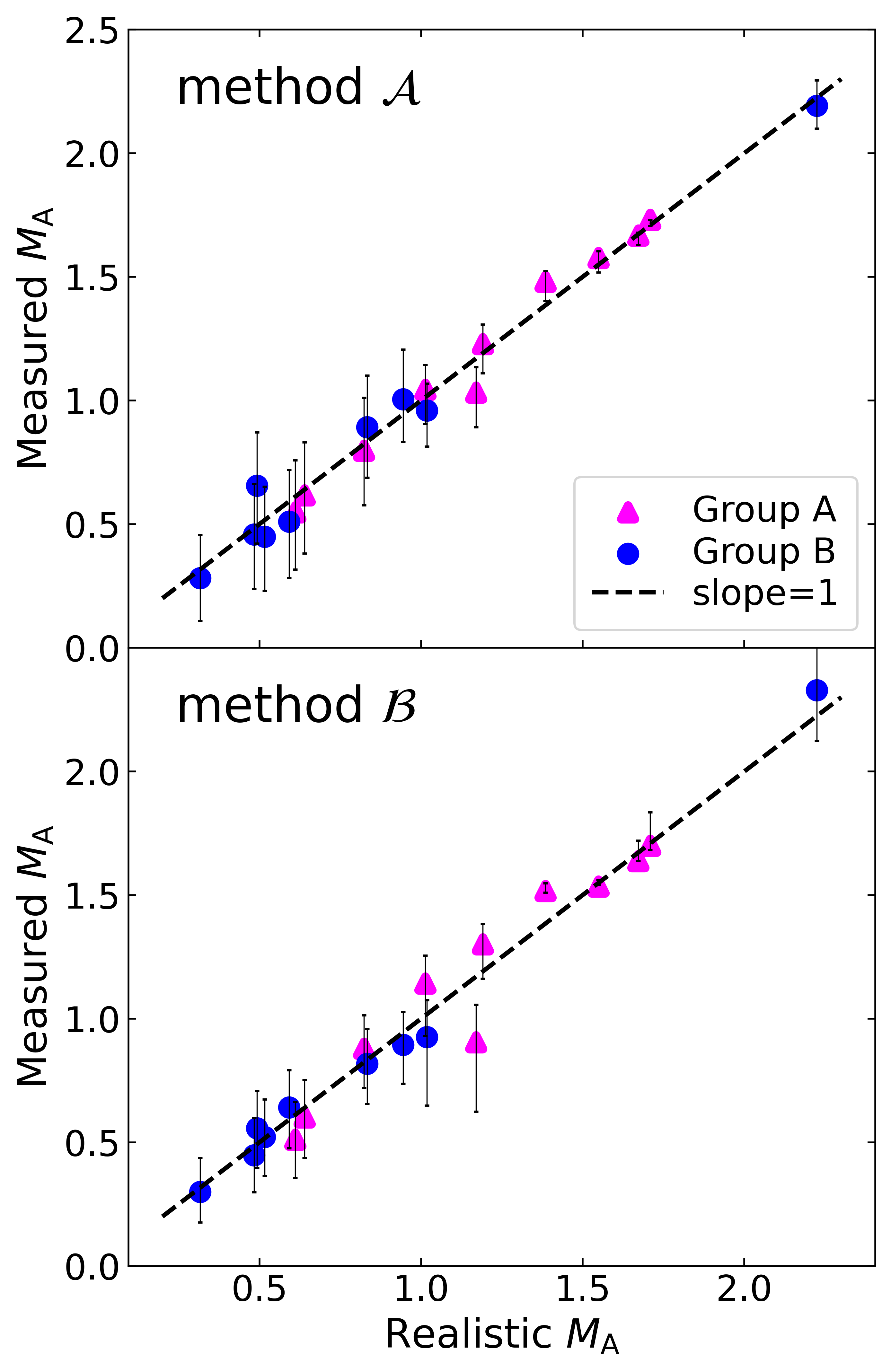
To test the reliability of the measurements, we first apply the two techniques to the imaging data we obtained by MHD turbulence simulations. By knowing the values of in advance, we can compare their values with the measured by techniques. Figure 3 shows the results we obtained by polarization intensity variance (upper panel) and the polarization angle dispersion (lower panel). The error bars are calculated using the upper and lower error limits summarized in Table 2, which also indicates the range of fitting errors presented in Figure 2. From Figure 3, we can see that filled data points for circles and triangles are distributed near the dashed line with a slope equal to 1, which demonstrates that the measured by both methods is consistent with the realistic determined from 3D MHD turbulence simulations.
Consequently, the power-law relationships we obtained are reliable for measuring . Next, we apply the power-law relationships summarized in Table 2 to measure the magnetization of the Galactic ISM.
5 Application to Observations
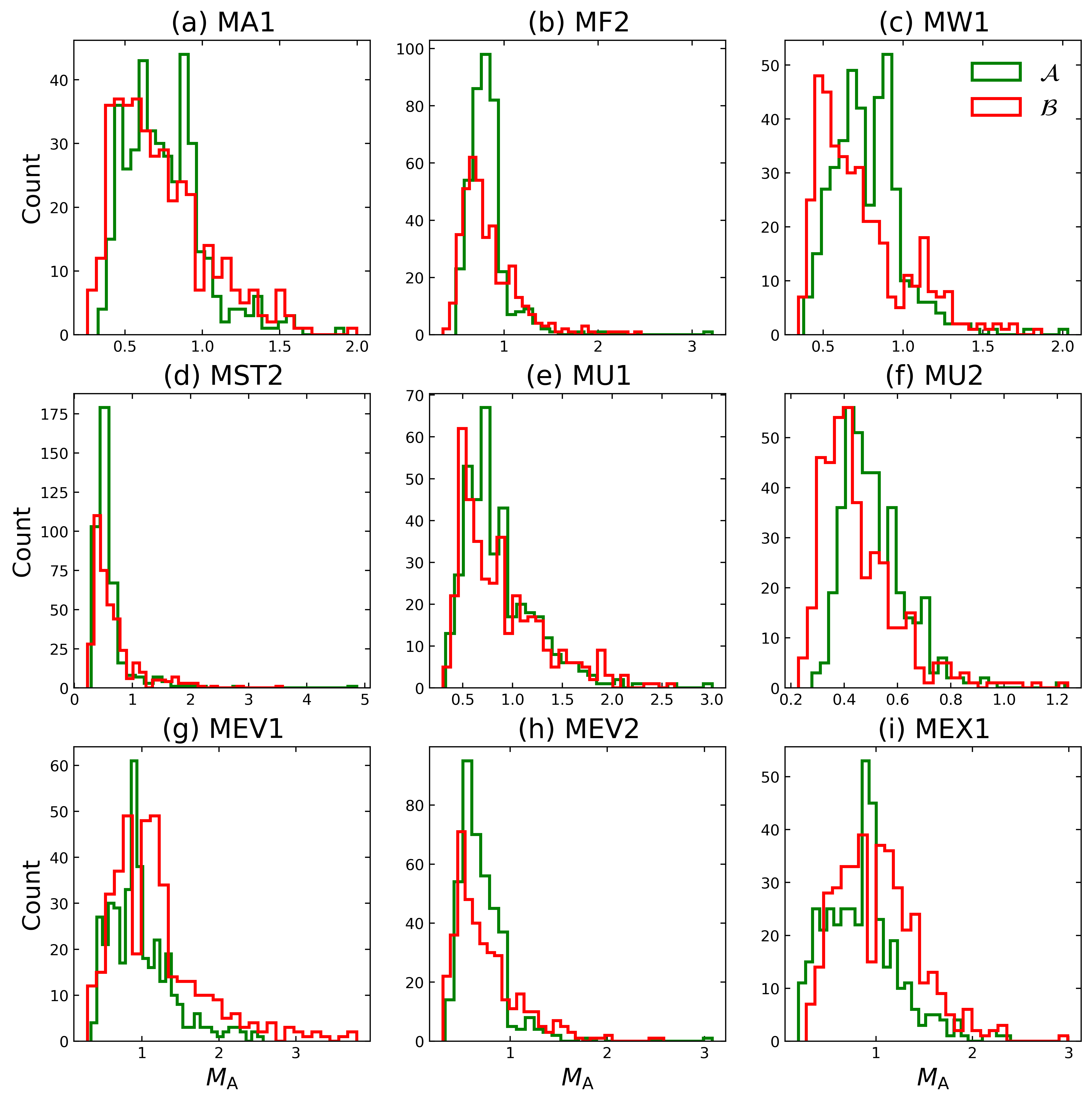
Here, we apply our techniques to the Canadian Galactic Plane Survey (CGPS) data with arcminute-scale images of all major components of the ISM over a large portion of the Galactic disk. Note that the Dominion Radio Astrophysical Observatory (DRAO) Synthesis Telescope surveys have imaged a section of the Galactic plane. The DRAO fields were combined into pixel mosaic images ( for each), with a resolution close to on a Galactic Cartesian grid at the 1.42 GHz. By randomly selecting 9 mosaics named MA1, MF2, MST2, MU1, MU2, MW1, MEV1, MEV2, and MEX1 (see Taylor et al. 2003 for detailed coordinate locations), we extract pixels, corresponding to the region of , from individual mosaic images to avoid the margin effect of the images (see also Zhang et al. 2019).
We consider a statistical average of different sub-regions from the whole mosaic image to measure expected from the whole mosaic image. In practice, we first decompose the selected mosaic image into 400 and 256 sub-block regions, which correspond to and pixels, respectively. Then, we employ the power-law relationships summarized in Table 2 to obtain the values of each sub-block region. Finally, we obtain statistical measurements of for all sub-regions to characterize the magnetization of the whole mosaic image.
The measurement results using pixels are plotted in Figures 4, from which we can see that histogram distributions from methods and are approximately consistent. To obtain quantitative values, we characterize the measurement for each mosaic image by the average and peak values of histogram distributions. Fitting the distribution histogram with the Gaussian function at a confidence level, we obtained the average and peak values of the distribution for each mosaic image.
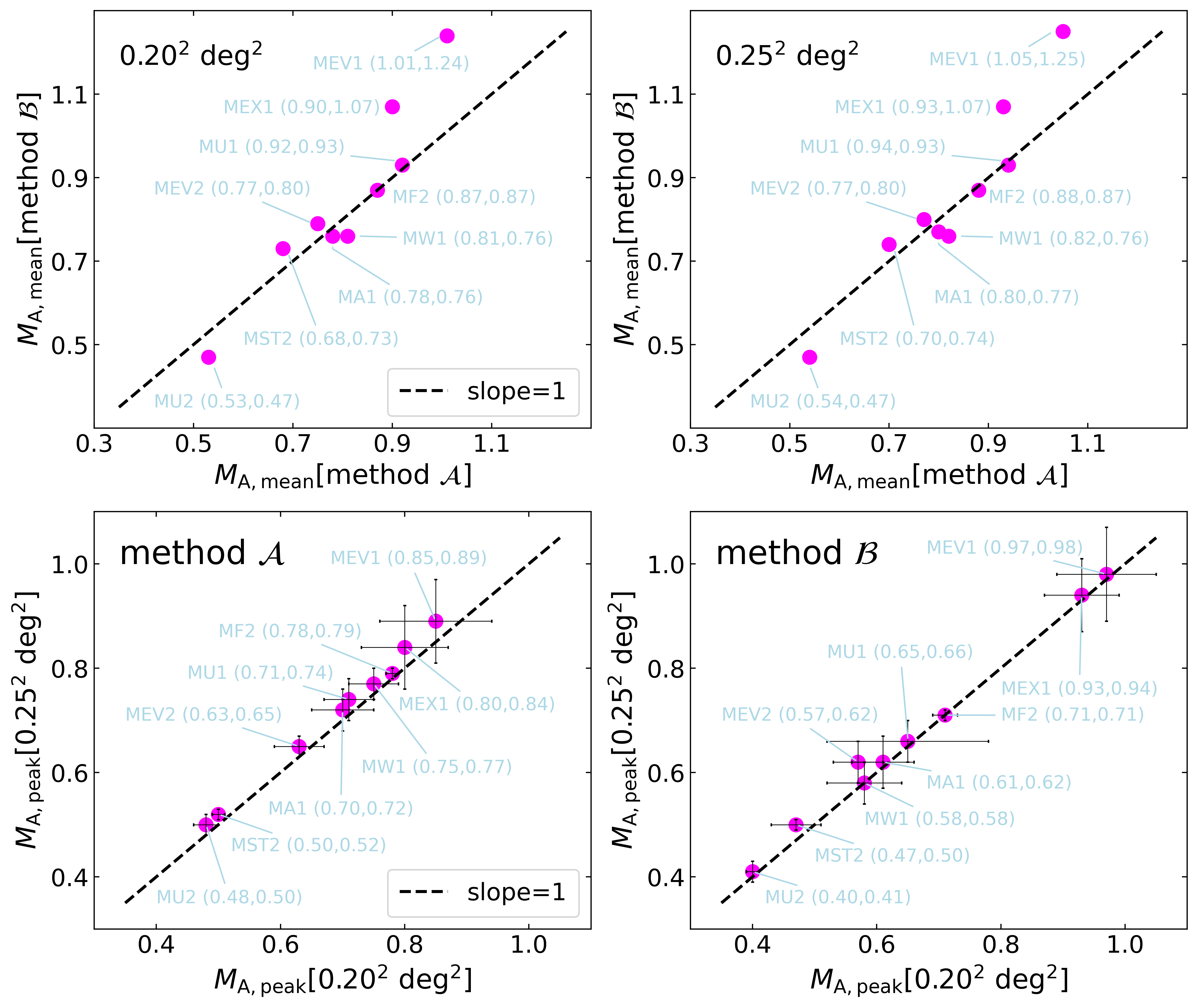
The upper panels of Figure 5 show the comparison of the average values measured by methods and when selecting different sub-region sizes. As seen in the upper panels, the results measured by the two methods are relatively similar in most regions, except that the results of method are about 0.1 larger for the MEV1 and MEX1 mosaics. This result shows that on the one hand, the measurement results of method are more reliable, and on the other hand, the size of the selected sub-region has no effect on measurements featured by average values. The lower panels of Figure 5 compare the distribution peak values of the same method when changing the size of the sub-region sizes, with the error bar plotted by a Gaussian function fitting error. It can be seen that the measurement results of methods and are the same in different sub-region sizes, indicating that the choice of sub-region size has little effect on the measurement results of . As a result, we propose that the low-latitude Galactic ISM is mainly dominated by sub-Alfvénic turbulence, with a magnetization level approximately between 0.5 and 1.0.
6 Discussion
Our current work has explored how polarization intensity variance can be used to measure the ISM magnetization, confirming the feasibility of this method. Considering the influence of Faraday depolarization on the measurement method, we find that in the explored parameter space, even if the polarization angle rotation reaches radians (see Figure 1), the power-law relation we established is less affected by the Faraday rotation effect, that is, only the fitting error variation of Bayesian statistics (see Table 2).
To further confirm the complementarity of the polarization intensity variance measurements, we have also tested other methods such as the top-base ratio from polarization gradient statistics, inverted variance method, and polarization degree dispersion. These methods have been explored in Lazarian et al. (2018) and Carmo et al. (2020). Our testing results are similar to Figure 7 of Lazarian et al. (2018) using the Galactic Arecibo L-band Feed Array data. Note that the measurement of the polarization degree dispersion often provides a smaller measurement value, because the Faraday rotation effect will result in a relatively low observed polarization degree.
We would like to emphasize that our current work is based on the framework of the modern understanding of MHD turbulence theory. The established power-law relationship is confined to the strong turbulence regime of the MHD turbulence cascade (see Section 2.1), that is, we ensure that the MHD simulation dataset listed in Table 1 has a sufficiently wide inertial range, with and greater than (see Equations (2) and (5)). For polarization angle dispersion, our results arising from compressible turbulence show the power-law relation of and in the sub- and super-Alfvénic regimes, respectively. Differently, Skalidis et al. (2021) and Lazarian et al. (2023) claimed that the polarization angle dispersion maintains the relation of for incompressible turbulence, and for compressible turbulence. What we would like to clarify is that their polarization dispersion is defined as , which is different from our definition in Equation (13). Note that Falceta-Gonçalves et al. (2008) mentioned that the polarization angle dispersion may be related to the angle between the LOS direction and the mean magnetic field. In our work, we do not consider the influence of the angle between the LOS and the mean magnetic field on our new method; this will be explored in the future.
In general, when the brightness temperature approaches the thermal temperature of relativistic electrons, the synchrotron self-absorption effect is expected to be important at low frequencies (Zhang & Wang, 2022). However, our testing shows that this radiative transfer process is negligible for the parameters used in this paper. In addition, it is not important for the effects of nonadiabatic propagation for Faraday rotation in the Galactic ISM (Lee et al., 2019).
7 Summary
In this work, we proposed a new method, polarization intensity variance, for measuring ISM magnetization. After confirming the reliability of the new technique using numerical simulation data, we applied the technique to measure the Galactic ISM magnetization with real observations. The main results are summarized as follows.
-
•
We proposed that polarization intensity variance can achieve accurate measurement of the ISM magnetization. Compared with the polarization angle dispersion method, we verify the reliability of the polarization intensity variance method in measuring the ISM magnetization.
-
•
We found a power-law relationship of between polarization intensity variance and magnetization . For the polarization angle dispersion, the power-law relationships are in the sub-Aflvénic turbulence and in the super-Aflvénic turbulence.
-
•
Using simulation polarization data with the known values, we demonstrated that polarization intensity variance can successfully recover the underlying magnetization , supporting the applicability of this new method.
-
•
With the application of polarization intensity variance, we propose that the low-latitude Galactic ISM is dominated by sub-Alfénic turbulence, with approximately between 0.5 and 1.0.
References
- Armstrong et al. (1995) Armstrong, J. W., Rickett, B. J., & Spangler, S. R. 1995, ApJ, 443, 209, doi: 10.1086/175515
- Beck & Wielebinski (2013) Beck, R., & Wielebinski, R. 2013, in Planets, Stars and Stellar Systems. Volume 5: Galactic Structure and Stellar Populations, ed. T. D. Oswalt & G. Gilmore, Vol. 5, 641, doi: 10.1007/978-94-007-5612-0_13
- Bourke et al. (2001) Bourke, T. L., Myers, P. C., Robinson, G., & Hyland, A. R. 2001, ApJ, 554, 916, doi: 10.1086/321405
- Brandenburg & Lazarian (2013) Brandenburg, A., & Lazarian, A. 2013, Space Sci. Rev., 178, 163, doi: 10.1007/s11214-013-0009-3
- Burn (1966) Burn, B. J. 1966, MNRAS, 133, 67, doi: 10.1093/mnras/133.1.67
- Carmo et al. (2020) Carmo, L., González-Casanova, D. F., Falceta-Gonçalves, D., et al. 2020, ApJ, 905, 130, doi: 10.3847/1538-4357/abc331
- Chandrasekhar & Fermi (1953) Chandrasekhar, S., & Fermi, E. 1953, ApJ, 118, 113, doi: 10.1086/145731
- Cho (2023) Cho, J. 2023, ApJ, 953, 114, doi: 10.3847/1538-4357/ace10a
- Cho & Lazarian (2002) Cho, J., & Lazarian, A. 2002, Phys. Rev. Lett., 88, 245001, doi: 10.1103/PhysRevLett.88.245001
- Cho & Yoo (2016) Cho, J., & Yoo, H. 2016, ApJ, 821, 21, doi: 10.3847/0004-637X/821/1/21
- Crutcher (1999) Crutcher, R. M. 1999, ApJ, 520, 706, doi: 10.1086/307483
- Crutcher et al. (2010) Crutcher, R. M., Wandelt, B., Heiles, C., Falgarone, E., & Troland, T. H. 2010, ApJ, 725, 466, doi: 10.1088/0004-637X/725/1/466
- Davis (1951) Davis, L. 1951, Physical Review, 81, 890, doi: 10.1103/PhysRev.81.890.2
- Elmegreen & Scalo (2004) Elmegreen, B. G., & Scalo, J. 2004, ARA&A, 42, 211, doi: 10.1146/annurev.astro.41.011802.094859
- Esquivel & Lazarian (2011) Esquivel, A., & Lazarian, A. 2011, ApJ, 740, 117, doi: 10.1088/0004-637X/740/2/117
- Esquivel et al. (2015) Esquivel, A., Lazarian, A., & Pogosyan, D. 2015, ApJ, 814, 77, doi: 10.1088/0004-637X/814/1/77
- Falceta-Gonçalves et al. (2008) Falceta-Gonçalves, D., Lazarian, A., & Kowal, G. 2008, ApJ, 679, 537, doi: 10.1086/587479
- Ginzburg & Syrovatskii (1965) Ginzburg, V. L., & Syrovatskii, S. I. 1965, ARA&A, 3, 297, doi: 10.1146/annurev.aa.03.090165.001501
- Goldreich & Sridhar (1995) Goldreich, P., & Sridhar, S. 1995, ApJ, 438, 763, doi: 10.1086/175121
- Goodman et al. (1989) Goodman, A. A., Crutcher, R. M., Heiles, C., Myers, P. C., & Troland, T. H. 1989, ApJ, 338, L61, doi: 10.1086/185401
- Hayes et al. (2006) Hayes, J. C., Norman, M. L., Fiedler, R. A., et al. 2006, ApJS, 165, 188, doi: 10.1086/504594
- Hernández-Padilla et al. (2020) Hernández-Padilla, D., Esquivel, A., Lazarian, A., et al. 2020, ApJ, 901, 11, doi: 10.3847/1538-4357/abad9e
- Hildebrand et al. (2009) Hildebrand, R. H., Kirby, L., Dotson, J. L., Houde, M., & Vaillancourt, J. E. 2009, ApJ, 696, 567, doi: 10.1088/0004-637X/696/1/567
- Houde et al. (2009) Houde, M., Vaillancourt, J. E., Hildebrand, R. H., Chitsazzadeh, S., & Kirby, L. 2009, ApJ, 706, 1504, doi: 10.1088/0004-637X/706/2/1504
- Hu et al. (2021) Hu, Y., Xu, S., & Lazarian, A. 2021, ApJ, 911, 37, doi: 10.3847/1538-4357/abea18
- Inoue (2023) Inoue, Y. 2023, PASJ, 75, L7, doi: 10.1093/pasj/psad017
- Kolmogorov (1941) Kolmogorov, A. 1941, Akademiia Nauk SSSR Doklady, 30, 301
- Larson (1981) Larson, R. B. 1981, MNRAS, 194, 809, doi: 10.1093/mnras/194.4.809
- Lazarian (2006) Lazarian, A. 2006, ApJ, 645, L25, doi: 10.1086/505796
- Lazarian et al. (2015) Lazarian, A., Eyink, G., Vishniac, E., & Kowal, G. 2015, Philosophical Transactions of the Royal Society of London Series A, 373, 20140144, doi: 10.1098/rsta.2014.0144
- Lazarian et al. (2023) Lazarian, A., HO, K. W., Yuen, K. H., & Vishniac, E. 2023, arXiv e-prints, arXiv:2312.05399, doi: 10.48550/arXiv.2312.05399
- Lazarian & Pogosyan (2016) Lazarian, A., & Pogosyan, D. 2016, ApJ, 818, 178, doi: 10.3847/0004-637X/818/2/178
- Lazarian & Vishniac (1999) Lazarian, A., & Vishniac, E. T. 1999, ApJ, 517, 700, doi: 10.1086/307233
- Lazarian et al. (2018) Lazarian, A., Yuen, K. H., Ho, K. W., et al. 2018, ApJ, 865, 46, doi: 10.3847/1538-4357/aad7ff
- Lazarian et al. (2022) Lazarian, A., Yuen, K. H., & Pogosyan, D. 2022, ApJ, 935, 77, doi: 10.3847/1538-4357/ac6877
- Lee et al. (2019) Lee, H., Cho, J., & Lazarian, A. 2019, ApJ, 877, 108, doi: 10.3847/1538-4357/ab1b1e
- Liu et al. (2021) Liu, J., Zhang, Q., Commerçon, B., et al. 2021, ApJ, 919, 79, doi: 10.3847/1538-4357/ac0cec
- Mao et al. (2021) Mao, J., Britto, R. J., Buckley, D. A. H., et al. 2021, ApJ, 914, 134, doi: 10.3847/1538-4357/abfdc6
- McKee & Ostriker (2007) McKee, C. F., & Ostriker, E. C. 2007, ARA&A, 45, 565, doi: 10.1146/annurev.astro.45.051806.110602
- Patil et al. (2010) Patil, A., Huard, D., & Fonnesbeck, C. J. 2010, Journal of Statistical Software, 35, 1, doi: 10.18637/jss.v035.i04
- Pavaskar et al. (2023) Pavaskar, P., Yan, H., & Cho, J. 2023, MNRAS, 523, 1056, doi: 10.1093/mnras/stad1237
- Schlickeiser (2003) Schlickeiser, R. 2003, in Energy Conversion and Particle Acceleration in the Solar Corona, ed. L. Klein, Vol. 612, 230–260
- Skalidis et al. (2021) Skalidis, R., Sternberg, J., Beattie, J. R., Pavlidou, V., & Tassis, K. 2021, A&A, 656, A118, doi: 10.1051/0004-6361/202142045
- Spangler & Spitler (2004) Spangler, S. R., & Spitler, L. G. 2004, Physics of Plasmas, 11, 1969, doi: 10.1063/1.1687688
- Taylor et al. (2003) Taylor, A. R., Gibson, S. J., Peracaula, M., et al. 2003, AJ, 125, 3145, doi: 10.1086/375301
- Xu & Hu (2021) Xu, S., & Hu, Y. 2021, ApJ, 910, 88, doi: 10.3847/1538-4357/abe403
- Zhang et al. (2016) Zhang, J.-F., Lazarian, A., Lee, H., & Cho, J. 2016, ApJ, 825, 154, doi: 10.3847/0004-637X/825/2/154
- Zhang et al. (2018) Zhang, J.-F., Lazarian, A., & Xiang, F.-Y. 2018, ApJ, 863, 197, doi: 10.3847/1538-4357/aad182
- Zhang et al. (2019) Zhang, J.-F., Liu, Q., & Lazarian, A. 2019, ApJ, 886, 63, doi: 10.3847/1538-4357/ab4b4a
- Zhang & Wang (2022) Zhang, J.-F., & Wang, R.-Y. 2022, Frontiers in Astronomy and Space Sciences, 9, 869370, doi: 10.3389/fspas.2022.869370