Tuning the electronic and magnetic properties of NiBr₂ via pressure

Abstract

Transition metal dihalides (MX₂, M= transition metal, X= halide) have attracted much attention recently due to their intriguing low-dimensional magnetic properties. Particular focus has been placed in this family in the context of multiferroicity– a common occurrence in MX₂ compounds that adopt non-collinear magnetic structures. One example of helimagnetic multiferroic material in the dihalide family is represented by NiBr₂. Here, we study the evolution of the electronic structure and magnetic properties of this material under pressure using first-principles calculations combined with Monte Carlo simulations. Our results indicate there is significant magnetic frustration in NiBr₂ due to the competing interactions arising from its underlying triangular lattice. This magnetic frustration increases with pressure and is at the origin of the helimagnetic order. Further, pressure causes a sizable increase in the interlayer interactions. Our Monte Carlo simulations show that a large (3-fold) increase in the helimagnetic transition temperature can be achieved at pressures of around 15 GPa. This indicates that hydrostatic pressure can indeed be used as a tuning knob to increase the magnetic transition temperature of NiBr₂.

I Introduction

Two-dimensional (2D) van der Waals (vdW) magnets have been intensively studied as they provide powerful platforms to explore novel physical phenomena and to implement intriguing applications Blei et al. (2021); Gibertini et al. (2019). Transition metal dihalides represent an emerging class of 2D vdW magnets that can exhibit multiferroic order and non-collinear spin textures McGuire (2017). Within this family, the magnetic semiconductor NiI₂ has been the subject of much research in recent yearsAmoroso et al. (2020); Ju et al. (2021); Song et al. (2022); Fumega and Lado (2022); Lebedev et al. (2023); Das et al. (2024). In the bulk, two magnetic phase transitions take place in this material: one at 75 K to a collinear antiferromagnetic (AFM) state and one at 60 K to a helimagnetic state Billerey et al. (1977, 1980). This noncollinear magnetic state simultaneously hosts a spin-induced ferroelectric polarization tunable with magnetic field, making NiI₂ a type-II multiferroic Kurumaji et al. (2013a). Recently, it has been demonstrated that the multiferroic phase in NiI₂ persists from the bulk to the single-layer limit Song et al. (2022). Further, it has been shown that a significant enhancement of the helimagnetic order in bulk NiI₂ can be achieved with hydrostatic pressure Occhialini et al. (2023); Kapeghian et al. (2024) all the way up to 132 K at 5 GPa.

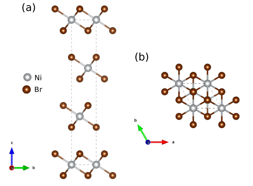
Figure 1: Crystal structure of bulk NiBr₂. Out-of-plane (a) and in-plane (b) views of the $R\overline{3}m$ structure. Ni atoms are represented by gray spheres, while brown spheres represent Br atoms. A black dotted line marks the unit cell boundaries.

Given that 2D multiferroics would provide disruptive possibilities to electrically control magnetic order, it is interesting to further explore other candidate materials in this context. An obvious choice is NiBr₂, a related compound from the dihalide family. NiBr₂ crystallizes in a CdCl₂ structure (space group $R\overline{3}m$)Day et al. (1976); Nasser et al. (1992) as depicted in Fig. 1. Its structure is formed by edge-sharing NiBr₆ octahedra (forming a triangular lattice) that stack along the $c$ axis with weak vdW bonding. The Ni²⁺ (S=1) Ni ions order antiferromagnetically at T_N,1 = 52 K Day et al. (1976); Day and Ziebeck (1980); Adam et al. (1980). As in NiI₂, this collinear AFM phase consists of ferromagnetic planes coupled antiferromagnetically out of plane. At T_N,2= 23 K, a second transition occurs to a spin-spiral orderDay and Ziebeck (1980); Adam et al. (1980). Interestingly, akin to NiI₂, NiBr₂ also develops a ferroelectric polarization in its helimagnetic low-temperature ground state Tokunaga et al. (2011). Notably, the helimagnetic transition temperature of NiBr₂ is considerably lower than that of NiI₂ but hydrostatic pressure could in principle be exploited as a means to enhance it.

Here, we study the effects of hydrostatic pressure on the magnetic properties of bulk NiBr₂ using a combination of first-principles calculations and Monte Carlo simulations. Our results indicate that there is a substantial magnetic frustration in NiBr₂ (that increases with pressure) arising from the competition between the intralayer ferromagnetic nearest-neighbor interaction ($J^{\parallel 1}$) and the antiferromagnetic third nearest-neighbor interaction ($J^{\parallel 3}$). Such magnetic frustration is at the origin of its helimagnetic ground state whose transition temperature we can accurately reproduce at ambient pressure using Monte Carlo simulations. We find that pressure has a significant effect on the interlayer coupling ($J^{\perp\mathrm{eff}}$), but also on some of the leading intralayer interactions. Using the first-principles-derived magnetic constants, Monte Carlo simulations reveal a 3-fold increase in the helimagnetic transition temperature of NiBr₂ at a modest pressure of 15 GPa.

II Computational Methods

First-Principles Calculations. We conducted density functional theory (DFT)-based calculations in NiBr₂ using the projector augmented wave (PAW) method Kresse and Joubert (1999) as implemented in the VASP code Kresse and Furthmüller (1996a, b). The wave functions were expanded in the plane-wave basis with a kinetic-energy cut-off of 500 eV. We considered the $3p$, $3d$, and $4s$ orbitals ($3p^{6}3d^{8}4s^{2}$ configuration) as valence states for the Ni atoms. Meanwhile, for the Br atoms, we considered the $4s$ and $4p$ orbitals ($4s^{2}4p^{5}$ configuration) as valence states.

Hydrostatic pressure was applied in 5 GPa increments (up to 15 GPa), conducting full structural relaxations. The optimization of the bulk unit cells at each pressure involved optimizing atomic positions, cell shape, and cell volume, but focusing exclusively on the rhombohedral phase. The energy and force minimization tolerances were set at $10^{-10}$ eV and $10^{-3}$ eV/Å, respectively. The calculations were done using the Perdew-Burke-Ernzerhof (PBE) Perdew et al. (1996) version of the generalized gradient approximation (GGA) functional, with the inclusion of the DFT-D3 van der Waals correction Grimme et al. (2010). Additionally, we incorporated an on-site Coulomb repulsion parameter ($U$) using the Liechtenstein Liechtenstein et al. (1995) approach to account for correlation effects in the Ni-$d$ electrons Rohrbach et al. (2003). The $U$ and Hund’s coupling $J_{\mathrm{H}}$ values utilized in all the calculations presented in the main text ($U=3.9$ eV and $J_{\mathrm{H}}=0.79$ eV) were derived from constrained random phase approximation (cRPA) calculations Riedl et al. (2022). For all of the relaxations, we fixed the magnetic configuration to an AFM state comprised of FM planes coupled AFM out of plane. To accommodate the AFM ordering, we employed a $1\times 1\times 2$ supercell and conducted Brillouin zone (BZ) sampling using a $40\times 40\times 4$ Monkhorst-Pack k-mesh centered on the $\Gamma$ point. This AFM order aligns with the $c$-component of the magnetic propagation vector ($\sim$ 3/2) McGuire (2017).

Finally, we computed the exchange couplings and anisotropies for NiBr₂ using the four-state method, extensively detailed in Refs. [Xiang et al., 2013, 2011a; Šabani et al., 2020; Xu et al., 2018, 2020]. This method relies on performing total energy mappings through noncollinear magnetic DFT calculations with spin-orbit coupling (SOC). Each magnetic interaction parameter is associated with the energies of four distinct magnetic configurations, wherein the directions of the magnetic moments are constrained, and large supercells are employed to prevent coupling between distant neighbors. Using this methodology, intralayer (interlayer) magnetic constants were calculated for each pressure.

Monte Carlo Simulations. We employed the Matjeset al. code to conduct Monte Carlo simulations in NiBr₂ to further investigate its magnetic response with pressure. Around $\sim 10^{6}$ thermalization steps were executed at each temperature, followed by $\sim 10^{4}$ Monte Carlo steps for statistical averaging. The simulations utilized a standard Metropolis algorithm on supercells with dimensions $L\times L\times 4$ and periodic boundary conditions. To determine the supercell size $L$, we adopted the criterion $L\simeq nL_{\mathrm{m.u.c.}}$, where $n$ is an integer, and $L_{\mathrm{m.u.c.}}$ represents the minimum lateral size of the magnetic unit cell. The length of the magnetic unit cell $L_{\mathrm{m.u.c.}}$ was estimated as $L_{\mathrm{m.u.c.}}\sim 1/q^{\parallel}$, where $q^{\parallel}$ denotes the magnitude of the in-plane component of the magnetic propagation vector derived as $q^{\parallel}=\frac{1}{2\pi}\arccos{\left[\left(1+\sqrt{1-2(J^{\parallel 1}/J^{\parallel 3})}\right)/4\right]}$Hayami et al. (2016); Batista et al. (2016).

III Results

We start by introducing the microscopic model that we will follow to obtain the relevant magnetic interactions for NiBr₂, given by the following Heisenberg Hamiltonian between localized spins S_i that we split into intra- and interlayer contributions expressed as $H^{\parallel}$ and $H^{\perp}$, respectively,

$$H^{\parallel}=\frac{1}{2}\sum_{i\neq j}\mathbf{S}_{i}\cdot\mathbf{J}^{\parallel}_{ij}\cdot\mathbf{S}_{j}+\sum_{i}\mathbf{S}_{i}\cdot\mathbf{A}_{i}\cdot\mathbf{S}_{i},$$ (1)

$$H^{\perp}=\frac{1}{2}\sum_{i,j}J^{\perp}_{ij}\mathbf{S}_{i}\cdot\mathbf{S}_{j},$$ (2)

Here, the indices $i$ and $j$ refer to the Ni atom sites. In Eq. 1, A_i denotes the on-site or single-ion anisotropy (SIA) and J_ij represents the intralayer exchange coupling interaction tensor. The latter can be decomposed into two contributions for NiBr₂: an isotropic coupling term, and an anisotropic symmetric term (the antisymmetric term which corresponds to the Dzyaloshinskii–Moriya interaction vanishes in NiBr₂ due to the presence of inversion symmetry). $J^{\perp}_{ij}$ in Eq. 2 represents the isotropic interlayer exchange constant between spins $\mathbf{S}_{i,j}$. We consider up to third nearest-neighbor isotropic exchanges both in-plane and out-of-plane. The full tensor is only taken into account for the in-plane nearest-neighbor exchange interaction. The factors of 1/2 are used to account for double-counting. The sign conventions used here are as follows: a positive (negative) isotropic exchange interaction favors an antiparallel (parallel) alignment of spins and a positive (negative) scalar single-ion parameter indicates an easy-plane (easy-axis) anisotropy.

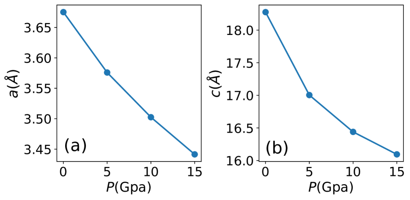
Figure 2: First-principles derived (a) in-plane and (b) out-of-plane relaxed lattice parameters as a function of pressure (P) for bulk NiBr₂.

Before moving into the evolution of the relevant magnetic parameters, we start by describing the evolution of the structural properties of NiBr₂ under pressure. Figure 2 displays the relaxed lattice parameters of NiBr₂ as a function of pressure obtained from our first-principles calculations using the computational parameters described in Section II. Upon applying hydrostatic pressure, both the in-plane (see Fig. 2(a)) and out-of-plane (see Fig. 2(b)) lattice parameters decrease monotonically, with a much larger decrease in the out-of-plane lattice parameter, as expected for a van der Waals material. Specifically, $a$ decreases from 3.67 Å  at ambient pressure to 3.44 Å  at 15 GPa while $c$ decreases from 18.27 Å to 16.09 Å at 15 GPa.

The basic evolution of the electronic structure is shown in Appendix A. Up to the highest pressures studied here, NiBr₂ remains insulating within our GGA+$U$ calculations (the gap can only be closed at $\sim$ 80 GPa). The derived magnetic moment for the Ni atoms is $\sim 1.54~{}\mu_{\mathrm{B}}$ at all pressures, consistent with high-spin Ni²⁺ but with a slightly reduced value with respect to the nominal one due to hybridization with the Br ligands (with moments $\sim 0.17\,\mu_{\mathrm{B}}$ at all pressures). Our first-principles derived magnetic moments are in good agreement with the ordered experimental Ni moment values obtained at ambient pressure $\sim 1.5\,\mu_{\mathrm{B}}$ Bikaljevic et al. (2021); McGuire (2017).

Isotropic intralayer exchanges
$P$	$J^{\parallel 1}$	$J^{\parallel 2}$	$J^{\parallel 3}$	$J^{\parallel 3}/J^{\parallel 1}$
0	-3.19	-0.05	1.56	-0.49
5	-3.71	-0.06	2.25	-0.61
10	-4.24	-0.14	2.92	-0.69
15	-4.68	-0.17	3.74	-0.8

SIA and intralayer TSA
$P$	$A$	$J^{\mathrm{S}\parallel 1}_{xx}$	$J^{\mathrm{S}\parallel 1}_{yy}$	$J^{\mathrm{S}\parallel 1}_{zz}$	$J^{\mathrm{S}\parallel 1}_{yz}$	$J^{\mathrm{S}\parallel 1}_{yz}/J^{\parallel 1}$
0	0.0	-0.04	0.04	0.0	-0.06	0.019
5	0.0	-0.05	0.04	0.0	-0.07	0.018
10	0.0	-0.05	0.05	0.0	-0.07	0.018
15	0.03	-0.2	0.13	0.07	-0.08	0.017

Isotropic interlayer exchanges
$P$	$J^{\perp 1}$	$J^{\perp 2}$	$J^{\perp 3}$	$J^{\perp\mathrm{eff}}$	$J^{\perp 2}/J^{\parallel 1}$
0	0.01	0.62	0.17	0.96	-0.19
5	0.01	1.7	0.42	2.54	-0.46
10	0.02	2.84	0.67	4.19	-0.67
15	0.12	4.02	0.9	5.94	-0.85

Table 1: Calculated NiBr₂ isotropic intralayer exchange interactions (top panel), interlayer isotropic interactions (bottom panel), SIA (A), and first-nearest neighbor in-plane two-site anisotropy (TSA) constants (middle panel) in a cartesian $x,y,z$ reference system where $x$ was chosen to be parallel to the Ni-Ni bonding vector for different pressures ($P$). $J^{\perp eff}$ represents the effective interlayer exchange and is obtained as $J^{\perp 1}+J^{\perp 2}+2J^{\perp 3}$, where the coefficient in the last term arises because there are twice as many out-of-plane third nearest-neighbors as first- and second nearest-neighbors. Pressure is in units of GPa, and exchange constants are given in units of meV.

After establishing the basics of the evolution of the structure and electronic structure in the AFM collinear phase, next we move on to the calculations of the magnetic coupling constants for NiBr₂ using the four-state method (we followed the implementation used for other dihalides as described in Refs. Amoroso et al., 2020; Gorkan et al., 2023; Kapeghian et al., 2024). Table 1 presents the computed intralayer and interlayer magnetic parameters introduced in Eqs. 1 and 2, as well as relevant ratios between magnetic couplings for pressures up to 15 GPa. Fig 3(a) shows the evolution of these relevant magnetic exchange ratios as a function of pressure while Fig 3(b) shows the paths for the dominant exchange interactions. At ambient pressure, the largest exchange interaction in NiBr₂ is the ferromagnetic (FM) intralayer first nearest-neighbor exchange ($J^{\parallel 1}$ $\sim$ -3.2 meV). The second nearest-neighbor exchange is vanishingly small and FM, while the third nearest-neighbor intralayer exchange is AFM and sizable ($J^{\parallel 3}$ $\sim$ 1.6 meV). The derivation of a large $J$ for third (vs. second) nearest-neighbors is consistent with previous results obtained for dihalide monolayers in Ref. Riedl et al., 2022: for second nearest-neighbors, only the $t_{2g}$-$e_{g}$ hopping is relevant at $d^{8}$ filling, leading to a weak FM interaction, while for third nearest-neighbors, there are large $e_{g}$-$e_{g}$ hoppings that arise from hopping paths that are ligand-assisted. Importantly, the competition between intralayer FM $J^{\parallel 1}$ and AFM $J^{\parallel 3}$ (measured by the ratio $J^{\parallel 3}/J^{\parallel 1}=-0.5$) results in a strong magnetic frustration which favors the realization of the non-collinear magnetic ground state of NiBr₂ Rastelli et al. (1979). Another critical parameter in the context of magnetic exchanges is the ratio $J^{\mathrm{S}\parallel 1}_{yz}/J^{\parallel 1}$ which gauges the canting of the two-site anisotropy axes from the direction perpendicular to the layersAmoroso et al. (2020). This ratio is estimated to be very small in NiBr₂ $J^{\mathrm{S}\parallel 1}_{yz}/J^{\parallel 1}=0.019$. Moving to the interlayer exchange interactions, they are all AFM in nature with the second nearest-neighbor $J^{\perp 2}$ being the dominant one $\sim$ 0.6 meV. If we look at the ratio between the dominant intra- vs. interlayer interactions $J^{\perp 2}/J^{\parallel 1}$$\sim$ - 0.2 at ambient pressure.

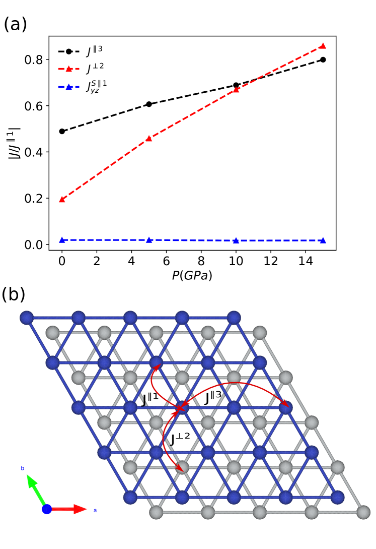
Figure 3: (a) Pressure evolution of the three relevant ratios of exchange couplings $J^{\parallel 3}$/$J^{\parallel 1}$, $J^{\perp 2}$/$J^{\parallel 1}$, $J^{S\parallel 1}_{yz}$/$J^{\parallel 1}$ for bulk NiBr₂. (b) The paths for the dominant exchange interactions $J^{\parallel 1}$, $J^{\parallel 3}$ and $J^{\perp 2}$ are shown over the triangular arrangement of Ni atoms in NiBr₂ (with gray spheres corresponding to Ni atoms in the bottom layer and blue spheres to those in the top layer).

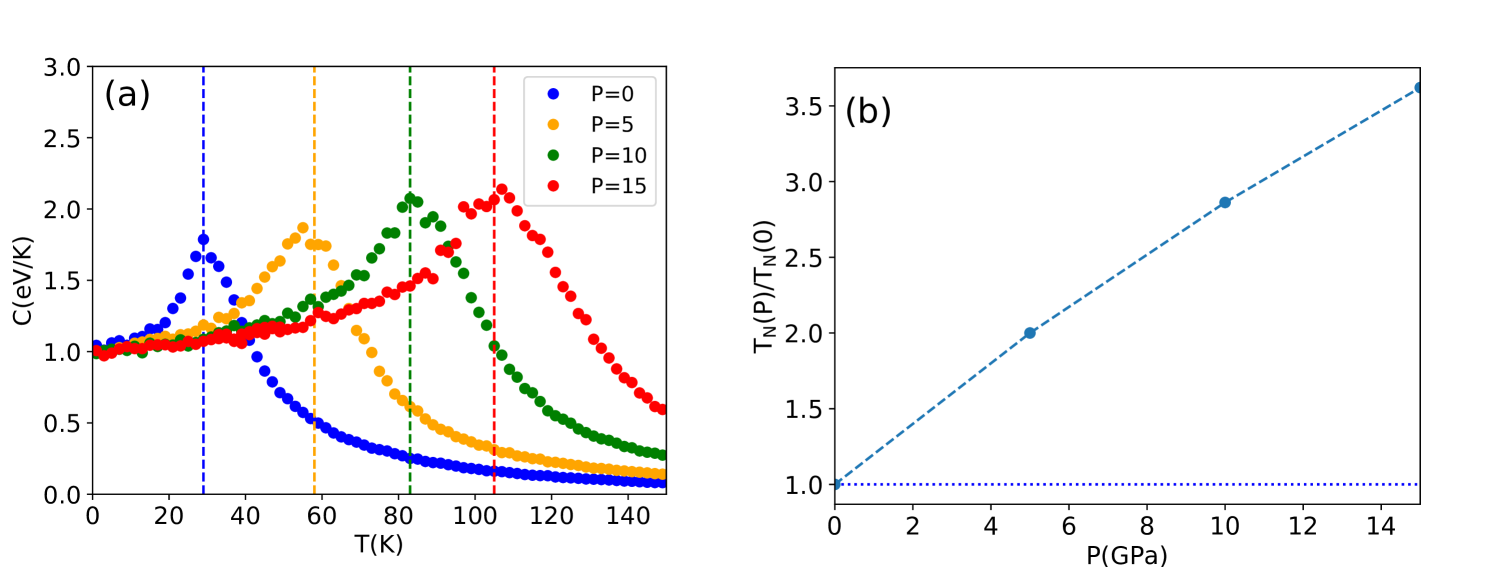
Figure 4: (a) Specific heat $C$ of bulk NiBr₂ as a function of temperature $T$ for various pressures P = 0, 5, 10, and 15 GPa obtained from Monte Carlo simulations. The dashed lines indicate the critical temperature $T_{\mathrm{N}}$ at each pressure: 29, 58, 83, and 105 K for 0, 5, 10, and 15 GPa, respectively. (b) Ambient-pressure-normalized critical temperature values for bulk NiBr₂ as a function of pressure $P$.

The signs of the dominant intra- and interlayer interactions do not change with pressure but the magnitude of the isotropic magnetic constants increases considerably. For the first nearest-neighbor isotropic exchange $J^{\parallel 1}$_15GPa= 1.5 $J^{\parallel 1}$_0GPa, for the third nearest-neighbor isotropic exchange $J^{\parallel 3}$_15GPa= 2.4 $J^{\parallel 3}$_0GPa, while the second nearest-neighbor $J^{\parallel 2}$ remains vanishingly small at all pressures. The pressure-dependent response of the dominant intralayer isotropic exchanges can be understood by looking at the relevant hopping amplitudes, as we showed before for NiI₂ Kapeghian et al. (2024). For $J^{\parallel 1}$ there are two primary contributions, one being FM (mainly arising from the hopping process between $t_{2g}$ and $e_{g}$ states via the ligand $p$ states) and the other AFM (mainly arising from direct $d-d$ overlap between Ni $t_{2g}$-like states). With increasing pressure, the FM contribution increases at a faster rate resulting in an overall increase of $J^{\parallel 1}$ even though the competition due to the AFM hoppings still persists. In contrast, $J^{\parallel 3}$ exhibits solely AFM contributions originating from $e_{g}$-$e_{g}$ hoppings, as mentioned above, without FM contributions. In this manner, the $J^{\parallel 3}/J^{\parallel 1}$ ratio undergoes a sizable increase with pressure from -0.5 at ambient pressure to -0.8 at 15 GPa (see Fig. 3(a)). The single-ion anisotropy is negligible at all pressures, and the intralayer anisotropic exchanges($J^{\mathrm{S}\parallel 1}_{yz}$) exhibit minimal changes with pressure as well. The ratio $J^{\mathrm{S}\parallel 1}_{yz}/J^{\parallel 1}$ remains nearly constant (and small) up to 15 GPa, as depicted in Fig. 3(a).

Regarding the interlayer exchanges, the signs of the dominant interlayer isotropic exchange interactions persist as well: both $J^{\perp 2}$ and $J^{\perp 3}$ remain antiferromagnetic in the pressure range studied here, even though they increase sizably with pressure ($J^{\perp 1}$ remains small in comparison). This substantial increase is particularly noticeable for the dominant second nearest-neighbor interlayer exchange $J^{\perp 2}$_15GPa= 6.5$J^{\perp 2}$_0GPa. Such a large increase can be attributed to the significant decrease in the $c$ lattice parameter with pressure described above, as expected in a vdW material. Importantly, $J^{\perp 2}$ at 15 GPa becomes the second largest interaction overall, closely competing in value with $J^{\parallel 1}$ (see Fig. 3(a)). In fact, if considering the overall effective interlayer exchange $J^{\perp\mathrm{eff}}$, it surpasses the dominant intralayer $J$ at $\sim$ 10 GPa as shown in Table 1.

The magnetic constants derived from the four-state method for NiBr₂ were subsequently used in Monte Carlo simulations. At low temperatures, we confirm that the derived magnetic ground state is a spin spiral (this is consistent with previous DFT-based studies that reported a spin-spiral ground state in monolayer NiBr₂Amoroso et al. (2021); Sødequist and Olsen (2023); Wu et al. (2023), see the corresponding magnetic texture and structure factor in Appendix B). From our pressure-dependent specific heat calculations we can clearly observe a magnetic transition at a temperature $T_{\mathrm{N}}$, indicated by the dashed vertical line in Fig. 4(a), that increases monotonically with pressure. Although some double-peak structure can be observed (that was also obtained in similar calculations for NiI₂Kapeghian et al. (2024)) we focus here on a qualitative understanding of the trends in the magnetic response with pressure, rather than pursuing a quantitative description of the two magnetic transitions (more rigorous statistical measures would be needed to assign physical meaning to the aforementioned double-peak structure, which we leave for future work). Fig. 4(b) clearly shows the monotonic increase of $T_{\mathrm{N}}$ as a function of pressure, with the data points being normalized relative to the value calculated at ambient pressure ($T_{\mathrm{N}}$(0 GPa)=29 K, very close to the experimentally derived value of $\sim$ 23 K). Notably, our calculated $T_{\mathrm{N}}$ undergoes a three-fold increase between 0 and 15 GPa (rising from 29 to 105 K).

Importantly, the increase in the $J^{\parallel 3}/J^{\parallel 1}$ ratio with pressure we have found in NiBr₂ has important implications for the helimagnetic propagation vector and likely for the related spin-induced ferroelectric polarization. As mentioned in Section II, the in-plane component of the magnetic propagation vector can be determined as $q^{\parallel}=2\arccos{\left[\left(1+\sqrt{1-2(J^{\parallel 1}/J^{\parallel 3})}\right)/4\right]}$, the related spin-induced ferroelectric order can be estimated as P $\propto$ sin($q$) by the generalized Katsura-Nagaosa-Balatsky model Kurumaji et al. (2013b); Song et al. (2022); Xiang et al. (2011b). The observed increase in $J^{\parallel 3}/J^{\parallel 1}$ with pressure favors a larger $q$ (shorter in-plane spiral pitch) which, potentially, can then give rise to a larger spin-induced polarization (see Appendix C for further details).

IV Summary

To summarize, we employed first-principles calculations combined with Monte Carlo simulations to investigate the impact of hydrostatic pressure on the magnetic properties of bulk NiBr₂. Using the four-state method, we computed the intralayer and interlayer exchange parameters (up to third nearest neighbors) of the low energy effective spin model for bulk NiBr₂. The low-temperature magnetic ordering corresponds to a spin spiral that is governed by the magnetic frustration between the two dominant in-plane exchange terms ($J^{\parallel 1}$ and $J^{\parallel 3}$), exhibiting different signs (ferro- and antiferromagnetic, respectively). The interlayer exchanges were identified as antiferromagnetic, with $J^{\perp 2}$ being the dominant interaction. With increasing pressure, all the dominating exchange couplings ($J^{\parallel 1}$, $J^{\parallel 3}$ and $J^{\perp 2}$) increase monotonically, and consequently, the (heli)-magnetic ordering temperature increases. These results suggest that hydrostatic pressure holds promise as a means to enhance the magnetic response of NiBr₂. Even though we do not analyze here the corresponding induced electric polarization, we anticipate that pressure could also potentially enhance the concomitant multiferroic response of NiBr₂.

V ACKNOWLEDGMENTS

SB, JK, OE and AB acknowledge support from NSF Grant No. DMR-2206987 and the ASU Research Computing Center for high-performance computing resources.

Appendix A Band Structure evolution with pressure for NiBr₂

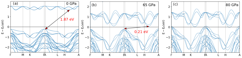
Figure 5: GGA-PBE+D3+$U$ band structure plots for bulk NiBr₂ (calculated with AFM order and $U=3.9$ eV) at ambient pressure (a), 65 GPa (b) and 80 GPa (c) where the energy band gaps are indicated in the insulating 0 and 65 GPa cases. Reciprocal space coordinates: $\Gamma=(0,0,0)$, $\mathrm{M}=(1/2,0,0)$, $\mathrm{K}=(1/3,1/3,0)$, $\mathrm{A}=(0,0,1/2)$, $\mathrm{L}=(1/2,0,1/2)$, $\mathrm{H}=(1/3,1/3,1/2)$

Fig 5 shows the evolution of the band structure along high-symmetry directions for NiBr₂ in the collinear an AFM state (consisting of ferromagnetic planes coupled antiferromagnetically out-of-plane) under hydrostatic pressure. The band gap can only be closed at $\sim$ 80 GPa.

Table 2 contains the corresponding indirect band gap $E_{gap}$ of bulk NiBr₂ as function of pressure.

$P$ (GPa)	Egap
0	1.8737
5	1.7282
10	1.5999
15	1.4630
40	0.8075
65	0.2137
80	0.0

Table 2: Indirect band gap $E_{gap}$ of bulk NiBr₂ as function of pressure. Here, a zero band gap value corresponds to a metallic state.

Appendix B Magnetization textures of monolayer NiBr₂

Fig 6(a) shows the magnetization texture of monolayer NiBr₂ ($10\times 10$ supercell) at P=0 and T=1 K, which exhibits a spin-spiral structure along the $x$ direction. The spin-spiral structure along the $x$ direction is confirmed by the spin structure factor data shown in Fig 6(b). The spin structure factor for momentum q is defined as

$$S(\textbf{q})=\frac{1}{N}\sum_{\alpha=x,y,z}\langle|\sum_{i}s_{i\alpha}e^{-i\textbf{q}\cdot\textbf{r}_{i}}|^{2}\rangle,$$ (3)

where N = $L^{2}$ is the total number of spins and $s_{i\alpha}$ denotes the $\alpha$ component of the spin at site i with position of the site $\textbf{r}_{i}$. This calculated spin structure factor is nonzero at two q points in momentum space.

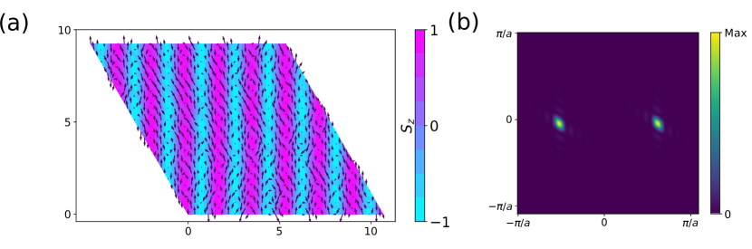
Figure 6: (a) Magnetization texture: black arrows represent the in-plane s_x, s_y spin components; the colormap indicates the out-of-plane s_z spin component and (b) Spin structure factor of monolayer NiBr₂ at ambient pressure at 1 K.

Appendix C Magnetic propagation vector

Table 3 contains the important exchange interaction ratio between $J^{\parallel 1}$ and $J^{\parallel 3}$ for bulk NiBr₂ for pressures up to 15 GPa. As mentioned in the main text, these exchange interactions are calculated using the four-state method. From this exchange interaction ratio, we calculate the in-plane component of the magnetic propagation vector $q^{\parallel}=\frac{1}{2\pi}\arccos{\left[\left(1+\sqrt{1-2(J^{\parallel 1}/J^{\parallel 3})}\right)/4\right]}$ which gives the magnetic unit cell size $L_{\mathrm{m.u.c.}}\sim 1/q^{\parallel}$ Hayami et al. (2016); Batista et al. (2016). With increasing pressure, the ratio $|J^{\parallel 1}$/$J^{\parallel 3}|$ decreases resulting in an increasing $q^{\parallel}$ with pressure. Such an increase in $q^{\parallel}$ with pressure corresponds to a decreasing $L_{\mathrm{m.u.c.}}$, which means that the magnetic unit cells gets smaller with increasing pressure.

$P$ (GPa)	$J^{\parallel 1}/J^{\parallel 3}$	$q^{\parallel}$	$L_{\mathrm{m.u.c.}}$
0	-2.05	0.098	10.14
5	-1.65	0.110	9.05
10	-1.45	0.116	8.59
15	-1.25	0.122	8.16

Table 3: Ratio of the leading intralayer exchanges $J^{\parallel 1}/J^{\parallel 3}$, in-plane component of the magnetic propagation vector magnitude $q^{\parallel}$, and magnetic unit cell length $L_{\mathrm{m.u.c.}}$ for bulk NiBr₂ at pressures ($P$) up to 15 GPa.

References

- Blei et al. (2021) M. Blei, J. L. Lado, Q. Song, D. Dey, O. Erten, V. Pardo, R. Comin, S. Tongay, and A. S. Botana, Applied Physics Reviews 8, 021301 (2021).
- Gibertini et al. (2019) M. Gibertini, M. Koperski, A. F. Morpurgo, and K. S. Novoselov, Nature Nanotechnology 14, 408 (2019).
- McGuire (2017) M. A. McGuire, Crystals 7 (2017), 10.3390/cryst7050121.
- Amoroso et al. (2020) D. Amoroso, P. Barone, and S. Picozzi, Nat Commun 11, 5784 (2020).
- Ju et al. (2021) H. Ju, Y. Lee, K.-T. Kim, I. H. Choi, C. J. Roh, S. Son, P. Park, J. H. Kim, T. S. Jung, J. H. Kim, K. H. Kim, J.-G. Park, and J. S. Lee, Nano Letters 21, 5126 (2021).
- Song et al. (2022) Q. Song, C. A. Occhialini, E. Ergeçen, B. Ilyas, D. Amoroso, P. Barone, J. Kapeghian, K. Watanabe, T. Taniguchi, A. S. Botana, S. Picozzi, N. Gedik, and R. Comin, Nature 602, 601 (2022).
- Fumega and Lado (2022) A. O. Fumega and J. L. Lado, 2D Materials 9, 025010 (2022).
- Lebedev et al. (2023) D. Lebedev, J. T. Gish, E. S. Garvey, T. K. Stanev, J. Choi, L. Georgopoulos, T. W. Song, H. Y. Park, K. Watanabe, T. Taniguchi, N. P. Stern, V. K. Sangwan, and M. C. Hersam, Advanced Functional Materials 33, 2212568 (2023).
- Das et al. (2024) J. Das, M. Akram, and O. Erten, Phys. Rev. B 109, 104428 (2024).
- Billerey et al. (1977) D. Billerey, C. Terrier, N. Ciret, and J. Kleinclauss, Physics Letters A 61, 138 (1977).
- Billerey et al. (1980) D. Billerey, C. Terrier, R. Mainard, and A. Pointon, Physics Letters A 77, 59 (1980).
- Kurumaji et al. (2013a) T. Kurumaji, S. Seki, S. Ishiwata, H. Murakawa, Y. Kaneko, and Y. Tokura, Phys. Rev. B 87, 014429 (2013a).
- Occhialini et al. (2023) C. A. Occhialini, L. G. P. Martins, Q. Song, J. S. Smith, J. Kapeghian, D. Amoroso, J. J. Sanchez, P. Barone, B. Dupé, M. J. Verstraete, J. Kong, A. S. Botana, and R. Comin, (2023), arXiv:2306.11720 [cond-mat.mtrl-sci] .
- Kapeghian et al. (2024) J. Kapeghian, D. Amoroso, C. A. Occhialini, L. G. P. Martins, Q. Song, J. S. Smith, J. J. Sanchez, J. Kong, R. Comin, P. Barone, B. Dupé, M. J. Verstraete, and A. S. Botana, Phys. Rev. B 109, 014403 (2024).
- Day et al. (1976) P. Day, A. Dinsdale, E. R. Krausz, and D. J. Robbins, Journal of Physics C: Solid State Physics 9, 2481 (1976).
- Nasser et al. (1992) J. Nasser, J. Kiat, and R. Gabilly, Solid State Communications 82, 49 (1992).
- Day and Ziebeck (1980) P. Day and K. R. A. Ziebeck, Journal of Physics C: Solid State Physics 13, L523 (1980).
- Adam et al. (1980) A. Adam, D. Billerey, C. Terrier, R. Mainard, L. Regnault, J. Rossat-Mignod, and P. Mériel, Solid State Communications 35, 1 (1980).
- Tokunaga et al. (2011) Y. Tokunaga, D. Okuyama, T. Kurumaji, T. Arima, H. Nakao, Y. Murakami, Y. Taguchi, and Y. Tokura, Phys. Rev. B 84, 060406 (2011).
- Kresse and Joubert (1999) G. Kresse and D. Joubert, Phys. Rev. B 59, 1758 (1999).
- Kresse and Furthmüller (1996a) G. Kresse and J. Furthmüller, Phys. Rev. B 54, 11169 (1996a).
- Kresse and Furthmüller (1996b) G. Kresse and J. Furthmüller, Computational Materials Science 6, 15 (1996b).
- Perdew et al. (1996) J. P. Perdew, K. Burke, and M. Ernzerhof, Phys. Rev. Lett. 77, 3865 (1996).
- Grimme et al. (2010) S. Grimme, J. Antony, S. Ehrlich, and H. Krieg, The Journal of Chemical Physics 132, 154104 (2010).
- Liechtenstein et al. (1995) A. I. Liechtenstein, V. I. Anisimov, and J. Zaanen, Phys. Rev. B 52, R5467 (1995).
- Rohrbach et al. (2003) A. Rohrbach, J. Hafner, and G. Kresse, Journal of Physics: Condensed Matter 15, 979 (2003).
- Riedl et al. (2022) K. Riedl, D. Amoroso, S. Backes, A. Razpopov, T. P. T. Nguyen, K. Yamauchi, P. Barone, S. M. Winter, S. Picozzi, and R. Valentí, Phys. Rev. B 106, 035156 (2022).
- Xiang et al. (2013) H. Xiang, C. Lee, H.-J. Koo, X. Gong, and M.-H. Whangbo, Dalton Trans. 42, 823 (2013).
- Xiang et al. (2011a) H. J. Xiang, E. J. Kan, S.-H. Wei, M.-H. Whangbo, and X. G. Gong, Phys. Rev. B 84, 224429 (2011a).
- Šabani et al. (2020) D. Šabani, C. Bacaksiz, and M. V. Milošević, Phys. Rev. B 102, 014457 (2020).
- Xu et al. (2018) C. Xu, J. Feng, H. Xiang, and L. Bellaiche, npj Computational Materials 4 (2018), 10.1038/s41524-018-0115-6.
- Xu et al. (2020) C. Xu, J. Feng, S. Prokhorenko, Y. Nahas, H. Xiang, and L. Bellaiche, Phys. Rev. B 101, 060404(R) (2020).
- (33) B. D. et al., “github.com/bertdupe/matjes,” .
- Hayami et al. (2016) S. Hayami, S.-Z. Lin, and C. D. Batista, Phys. Rev. B 93, 184413 (2016).
- Batista et al. (2016) C. D. Batista, S.-Z. Lin, S. Hayami, and Y. Kamiya, Reports on Progress in Physics 79, 084504 (2016).
- Bikaljevic et al. (2021) D. Bikaljevic, C. González-Orellana, M. Pena-Díaz, D. Steiner, J. Dreiser, P. Gargiani, M. Foerster, M. A. Nino, L. Aballe, S. Ruiz-Gomez, et al., ACS nano 15, 14985 (2021).
- Gorkan et al. (2023) T. Gorkan, J. Das, J. Kapeghian, M. Akram, J. V. Barth, S. Tongay, E. Akturk, O. Erten, and A. S. Botana, Phys. Rev. Mater. 7, 054006 (2023).
- Rastelli et al. (1979) E. Rastelli, A. Tassi, and L. Reatto, Physica B+C 97, 1 (1979).
- Amoroso et al. (2021) D. Amoroso, P. Barone, and S. Picozzi, Nanomaterials 11, 1873 (2021).
- Sødequist and Olsen (2023) J. Sødequist and T. Olsen, 2D Materials 10, 035016 (2023).
- Wu et al. (2023) D.-W. Wu, Y.-B. Yuan, S. Liu, M.-Q. Long, and Y.-P. Wang, Phys. Rev. B 108, 054429 (2023).
- Kurumaji et al. (2013b) T. Kurumaji, S. Seki, S. Ishiwata, H. Murakawa, Y. Kaneko, and Y. Tokura, Phys. Rev. B 87, 014429 (2013b).
- Xiang et al. (2011b) H. J. Xiang, E. J. Kan, Y. Zhang, M.-H. Whangbo, and X. G. Gong, Phys. Rev. Lett. 107, 157202 (2011b).