Laguerre-Gaussian light induction of orbital currents and Kapitza stabilization in superconducting circuits
Abstract
We investigate the effects of a Laguerre-Gaussian (LG) beam on the superconducting state. We show that the vortex angular momentum of a LG beam affects the superconducting state and induces currents. The induction of the current by light is illustrated on a Josephson loop and SQUID devices. In particular, we establish that coupling a dc SQUID to the AC magnetic flux of a LG beam can stabilize phase in the SQUID. This can happen via developing a global or local minimum in the effective potential at . In the latter case, this happens via the Kapitza mechanism.
I Introduction
The process of interaction of quantum fields where one transfers quantum numbers from one to another is a well known phenomenon in quantum mechanics. We focus on the specific case of transfer of quantum numbers of light to coherent electron quantum state. Examples of these transfer processes include energy, momentum, angular momentum transfers as illustrated, e.g., by light-induced momentum change of a particle and induction of magnetization due to circular polarization of the photons [1, 2, 3, 4, 5, 6, 7, 8] . Recently, it has been suggested that interaction of light carrying non-zero angular momentum can induce vortices in superconductors [9, 10, 11]
In this paper, we look at a newer example of the interaction of quantum matter with structured light and microwave radiation: the induction of the circular orbital motion of the superconducting electrons illuminated by the so-called Laguerre-Gaussian (LG) beam, see Eq. 1. A LG beam has the vortex in light field phase [12]. The assumption hence is that even in linear response the phase coherent superconducting (SC) electrons will develop a coherent response while interacting with the beam that carries vorticity. We indeed find that LG beams do induce SC currents. One can say that vorticity of the beam is imprinted on the coherent quantum fluid, in our case chosen to be SC fluid. Qualitative explanation of the effect is direct: to carry orbital momentum, an electromagnetic (EM) wave propagating in -direction must have its amplitude of the electric and magnetic fields to be dependent on coordinates, or in polar angle in case of LG beam, on which we concentrate. This means that -component of the magnetic field of the beam is non-zero. This results in non-zero flux through an area normal to the beam propagation, Fig. 1, which oscillates with the frequency of the LG beam.
The effect is expected to be present in broader contexts; here we choose to illustrate it on the SQUID - the SC device that contain loop currents that are interacting with the light.
To test these ideas one can use sensing of the induced flux by SQUID devices via Aharonov-Bohm like setup. We show that this can lead to the dynamically stabilized effective Josephson junction. While the effect we discuss has similarities with the Aharonov-Bohm effect, there is a key difference – in the light-induced flux, the light field needs to enter into a SC and hence plays the role of the physical field that is sampled by SC current. In the traditional Aharonov-Bohm effect, the magnetic field is nonzero inside the solenoid and does not enter into the superconductor. Hence, for the setups we consider, it is important that the light field directly “touches” the superconducting electron liquid.
The structure of the paper is as follows: we give a brief introduction into a LG beam in Section II. In Section III, we start with the simpler example of a magnetic field and flux induced by a LG beam in the SC loop. In Section IV, we expand the calculation to the dc SQUID geometry. In Section V, we consider the full nonlinear dynamics of the coupled light-SQUID setup and find that, with the proper tuning, one can induce Josephson phase shift as a stable point of the junction potential. We also elaborate on the light-induced Kapitza engineered junction. We conclude in Section VI.
II Magnetic flux generated by LG beams
To the zeroth order in the paraxial parameter, the electric field of a linearly polarized LG higher mode with a wavevector and wavelength propagating in -direction can be considered purely transverse and written as [13]
| (1) |
where is the radius-vector written in cylindrical coordinates, is a unit vector in -direction, and
| (2) | ||||
| (3) |
where is the spot size at , where is the Rayleigh range with being the refraction index of the medium, is the radius of curvature of the wavefront of the Gaussian beam at , is the Gouy phase, and is an integer corresponding to the order of the LG mode. In fact, -component of the electric field is not zero: From , it can be estimated that , which is small compared to in the paraxial approximation.
Correspondingly, the vector potential is the real part of
| (4) |
and the flux through a disk-area of radius normal to the beam propagation is
| (5) |
This simple observation implies the possibility of generating high-frequency oscillating electromotive force with a LG beam via Faraday effect. For modern lasers, such flux is rather small - on the order Wb, which is only times larger than the magnetic flux quantum, . However, the Josephson phase is sensitive to the magnetic flux which is on the order of , and in the next sections we study the interaction of such a flux from LG beams with superconducting rings with Josephson junctions (JJ).
We note that the flux is contour dependent, and specifically chosen contours for other type of beams also can contain non-zero flux. However, a circular-shaped contours look particularly convenient to us.
III A LG beam shone on a rf SQUID
We start with shining LG light into the orifice of an rf SQUID structure, see Fig. 1. In the following, we neglect the physics that can lead to Shapiro effect [14] due to the electric component of the EM wave and photon-assisted tunneling [15, 16]. This is a reasonable approximation if the JJs are positioned in such a way that the polarization of the electric field is perpendicular to the Josephson current through the junctions (i.e., it is parallel to the surfaces of the electrodes that constitute the junctions) and the power of the beam is sufficiently small.
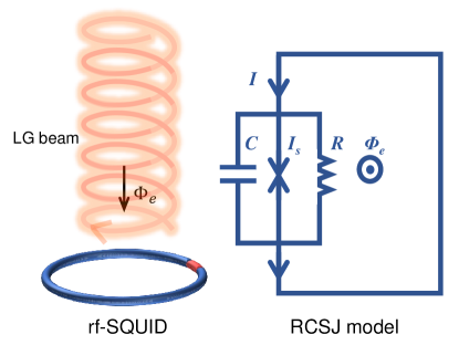
The RCSJ model for the dynamics of the rf SQUID then reads [17]
| (6) | ||||
where is the full flux through the orifice of the SQUID, , , and are the capacitance, resistance, and self-inductance of the rf SQUID, respectively, is the Josephson critical current, is the full current in the loop, and is the magnetic flux quantum. Combined, eqs. in Eq. 6 give
| (7) |
where , , , , and . This model with oscillating in time studied in [18, 19, 20] exhibits complex dynamic behavior including chaos.
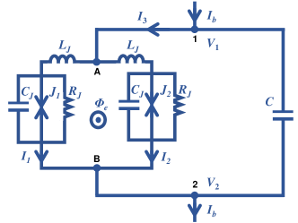
IV A LG beam is shone inside a dc SQUID shunted by an external capacitor
We can couple to the dynamic variable in the dc SQUID setup. Let us consider a symmetric dc SQUID shunted by an external capacitor as depicted in Fig. 2. We start with the simplest model neglecting the self-inductances of the electrodes comprising the dc SQUID and the capacitances and resistances of the JJs. In this case, the dc SQUID behaves effectively like a JJ with the amplitude of the Josephson critical current modulated by the external flux through the dc SQUID [21].
Indeed, the flux through the SQUID is
| (8) |
where are phase differences across the JJs, , and is the current circulating in the loop of the dc SQUID. Neglecting term in Eq. 8, the interference of the currents and through JJs gives
| (9) |
where .
Ultimately, we can think about the dc SQUID as an effective JJ with flux modulated critical current . Under the assumptions, the voltage across the SQUID is
| (10) |
Combinination of Eqs. 9 and 10, and , where is the charge on the shunting capacitor and is the bias current (which we do not show in Fig. 2) assumed to be constant, leads to the equation for analogous to the RCSJ model
| (11) |
where we have also added a dissipative term and , where .
We assume now, according to Eq. 5, the time-dependence for the external flux is cosinusoidal, such that with , and . Using the Jacobi–Anger expansion [22]
| (12) |
we rewrite Eq. 11 as
| (13) | ||||
which we recognize as an equation of an oscillator in a fast oscillating field. Then, for sufficiently large , we can expect the Kapitza-pendulum scenario [23, *kapitza1, 25, *kapitza2, 27], i.e., the stabilization upon drive of the formerly unstable state. We investigate such a possibility in the next section, where, based on the simple idea layed out in this section, we systematically study Kapitza-pendulum scenario in the dc SQUID geometry without shunting the SQUID by an external capacitor. The case with an external capacitor without neglecting the JJ’s capacitances and inductances is briefly discussed in Appendix A.
V dc SQUID
Based on the ideas in the previous section, we investigate the possibility of the Kapitza scenario in a dc SQUID subjected to the flux from a LG beam without it being shunted by an external capacitor. A vast literature is devoted to the study of dynamics in dc SQUIDs [28, 29, 30, 31, 32, 33, 34, 35]. Kapitza engineering [36, 37, 38, 39, 40] of a SQUID has not been widely discussed to date.
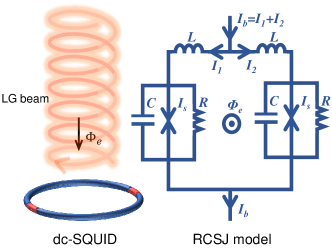
Consider an equivalent scheme of a symmetric dc SQUID depicted in Fig. 3. The relation for the flux and phases reads
| (14) |
where is the current circulating in the loop of the dc SQUID. For the time-dependent , this equation assumes instantaneous adjustment of the phases . This is approximately true if the time-scale on which changes is significantly slower than the relevant time-scale for the superconductor dynamics, , where and are the Plank constant and the superconducting order parameter, respectively.
The set of Kirhoff’s laws for currents reads
| (15) | |||
where is the bias current assumed to be constant. And the voltage across the dc SQUID is given by (see Appendix A for an example of the derivation)
| (16) |
Taking sum and difference of the first two equations in Eq. 15 and introducing notation , , , and , we obtain
| (17) | ||||
where is the full flux in units of and relates to via Eq. 14.
Note that the second equation in Eq. 17 is an equation for the flux inside the SQUID and is essentially the same as Eq. 7 for the dynamics of the flux inside an rf SQUID.
We can deem the considered system as a black-box device and ask a question about its I-V characteristic. Under typical assumption that is created by an external source of constant current, the output voltage, according to Eq. 16, is . Thus, in the Kapitza scenario of inverted pendulum, where oscillate around , such a black-box device may be considered as an effective -phase Josephson junction.
For , two equations in Eq. 17 decouple. We start with this case in the following section.
V.1 Neglecting the self-inductance:
When , is simply given by the external flux: . For generality, we will include a dc component of the external flux
| (18) |
Substituting this into the first equation in Eq. 17 and using the Jacobi-Anger expansion, we obtain
| (19) | ||||
where we also set . Non-zero cases then can be taken into account in the context of the washboard potential.
To investigate this, we employ the idea of separation of time scales [23, *kapitza1, 25, *kapitza2, 27]: given , we expect the solution can be described as a slowly varying component (on the scale of ) with small-amplitude fast oscillations (on the scale of ) on top of it 111An analytical method of wider applicability can be used [46], i.e., we represent
| (20) |
where and are the slow and fast components, respectively. Substituting this in Eq. 19, expanding in , and collecting the dominant fast terms together, we obtain an equation for
| (21) |
where we kept the dissipative term in Eq. 21 to incorporate the overdamped regime, . The solution for the fast component is
| (22) |
where the phase shifts satisfy . We set to comply with the physical picture of the solution (small-amplitude fast oscillations about the slow-mode component).
For the slow term, after averaging over time, we have
| (23) | |||
When , Eq. 23 is an equation of motion for a mathematical pendulum in an effective potential
| (24) |
where
| (25) |
This potential develops a local minimum at when . It is easy to see that such a condition can be satisfied for sufficiently close to the roots of the zero-order Bessel function of the first kind or/and for such that is sufficiently small. Simultaneously, the natural frequency of the oscillator in Eq. 23 becomes small, which allows for the Kapitza effect to occur at frequencies comparable to , the plasma frequency of the Josephson junction.
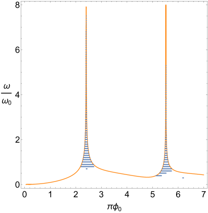
When , the coefficient in the third term in Eq. 23 becomes negative. This sign can be absorbed by shifting by in Eq. 23: . Correspondingly, the effective potential shifts by as well, moving the global minimum to . We call this regime the inverted pendulum regime. The Kapitza effect, i.e., the stabilization of the oscillation around the emergent local minimum, then is realized for . We call this regime the inverted Kapitza pendulum regime. Setting , we illustrate these regimes in Fig. 4, where we plot -vs- dependence at .
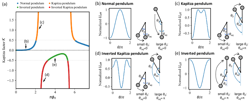
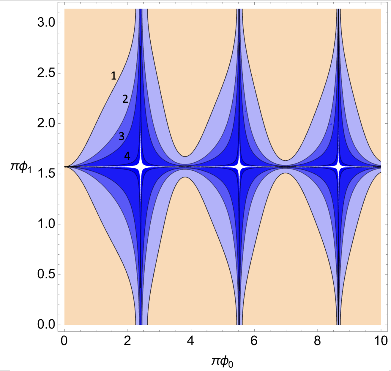
Found analytically under the assumptions explained above, Eq. 25 is not exact and does not allow to determine the smallest values of at which the Kapitza effect still occur. In Fig. 5, we plot a curve in - plane at at which and numerically determined region, where the Kapitza effect takes place. We see that the theoretical curve fit the numerically determined boundaries of Kapitza region quite well for sufficiently large . In Fig. 6, we plot curves in - plane for four values of : .
V.2 Relevant parameters of the LG beam
The model we have considered above have certain bounds of applicability. As follows from the discussion after Eq. 14, the frequency of should satisfy .
Considering typical in high-temperature superconductors being about K, the frequency of the LG beam then has to satisfy Hz, i.e., has to lie in the microwave range. Correspondingly, the wavelength of the LG beam is at least on the order of m. Consequently, the waist of the beam is also at least m. This would likely imply that in a realistic experiment the paraxial parameter is not small, and the formulas in Eqs. 1 and 2 are not quantitatively correct. Nevertheless, the value of the transverse component remains of the same order as the paraxial approximation predicts [42]. Thus, since the total flux through the ring is determined by the transverse component of the vector potential, we proceed with the estimation of the flux through the ring at (i.e., at the beam’s waist) using the electric field given by Eq. 1
| (26) |
where , which has a maximum at = 1.
According to Eq. 25, the smallest values of flux at which the Kapitza effect is observed is around , the first root of . And thus, from Eq. 26, we find that for this value is achieved at , which for Hz becomes V.
In the paraxial approximation, the total power of the LG mode is given by
| (27) |
which is the same formula as for the power of the fundamental Gaussian mode.
The power output of contemporary continuous-wave masers is much lower than that of lasers, typically on the order of picoWatts. For W, from Eq. 27, we obtain V, which is enough to achieve the desirable amount of flux. In case of a maser based on nitrogen vacancies in diamond, which produces one of the highest output power of W [43, 44], we estimate V.
V.3 The effect of self-inductance:
When , two equations in Eq. 17 are coupled. Here we discuss the results of numerical investigation of this set of equations at non-zero .
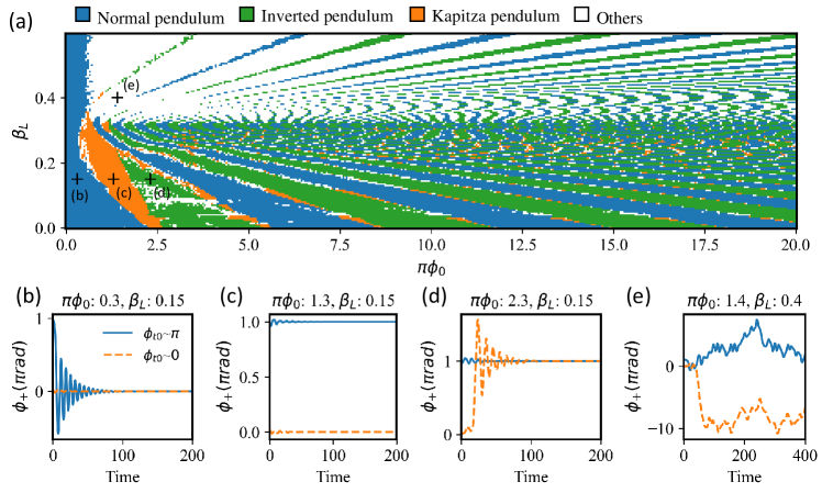
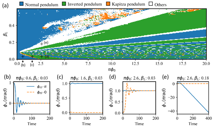
If is non-negligible, then the screening effect from the current inside the closed-loop SQUID circuit affects the dynamics of the effective phase . We utilize the Crank–Nicolson method to solve for the time trace of the phase and flux in Eq. 17. Adopting the screening parameter , we plot the phase diagram in terms of the normal, Kapitza (encompassing both the Kapitza and the inverted Kapitza), and inverted pendulum regimes in Figs. 7 and 8 for and , respectively, without distinguishing between the Kapitza and the inverted Kapitza regimes.
For both ratios of after small finite value of , the phase diagrams display ray-like structures of normal and inverted regimes with origins on the horizontal line at finite . These “rays” are separated by the “rays” with a mix of the Kapitza and “Other” regimes (see Figs. 7 and 8). Here, it is possible that some of the inclusions (especially in the lower part of the plots) of regions of “Other” regimes is due to instabilities in our numerical solutions. For ( for and for ), there is only normal pendulum regime of the dynamics of .
VI Conclusion and discussion
In this study we present the results for stirring of the circular motion of the superconducting fluid with structured light, a LG beam. In particular, we find Laguerre-Gaussian beams with provide non-zero AC magnetic flux through a disk-area of finite radius. This flux can be used to induce currents in superconducting rings and superconducting rings with Josephson junctions.
In the dc SQUID geometry, a SC ring with two JJ, we have found that coupling of periodic flux might lead to the Kapitza effect – the stabilization of oscillations about emergent local minimum at phase equal to . In the limit of negligible self-inductance, the ranges of the flux amplitude for which Kapitza effect is found are relatively narrow with the widest being the first one from zero flux. Numerical investigations suggest that these intervals for the Kapitza effect shift to smaller values of fluxes, and the width of such intervals can even enlarge (see Fig. 7). Unlike the case of the well-known mechanical oscillator, within the time-scales separation approach, the effect can be observed for driving frequencies that are on the order of the natural frequency, .
It is known that inverted regime of the oscillations of a dc SQUID, in which the global minimum shifts by , is achieved by biasing the SQUID with proper amount of DC flux. Here we have shown that analogical regime can be achieved with purely AC magnetic flux.
Our estimations suggest that the frequency of a LG beam should be in the microwave regime for the employed model to be correct. However, the effect might survive beyond the applicability of the model used. While the power output of current masers is much lower compared to that of lasers, we estimate that it is enough to produce the Kapitza effect. On the other hand, the model of the dynamics does not rely on the particular source of the AC magnetic flux, and the predicted dynamics can be tested in the lab with conventional electronics. The possibility of utilizing the Kapitza and inverted regime of a dc SQUID in applications, e.g., sensing, is not fully clear to us at this point.
The appearance of the local minimum in the effective potential allows to speculate about the possibility of utilizing it for constructing a novel Floquet-type qubit [45] based on Josephson junctions.
Based on a simple idea similar to the one explained in Section IV, we expect the possibility of stabilizing the effective phase at in an asymmetric dc SQUID. We will investigate such a possibility in a follow-up paper.
VII Acknowledgments
We are grateful to A. Dalal, G. Jotzu, I. Khaymovich, D. Kuzmanovski, I. Sochnikov, and P. Volkov for useful discussions. This work was supported by the European Research Council ERC HERO-810451 synergy grant, KAW foundation 2019-0068 and the Swedish Research Council (VR). Work at University of Connecticut was supported by the OVPR Quantum CT.
Appendix A A dc SQUID shunted by an external capacitor
In this section, we formulate the equations that govern the dynamics of a symmetric dc SQUID shunted by an external capacitor. The equivalent scheme is depicted in Fig. 9. The flux equation is
| (28) |
where is the current circulating in the dc SQUID loop. The Kirchhoff’s laws take the form
| (29) | ||||
| (30) | ||||
| (31) | ||||
| (32) |
where are the Josephson phases of the JJs , are currents through the JJs , is the total current through the dc SQUID, is the bias current assumed to be constant, , , and are the critical current, capacitance, and the resistance of JJs, is the self-inductance of the parts with JJs of the circuit between points A and B (see Fig. 9), and is the charge of the external capacitor , where are the voltages at points (see Fig. 9).
To find the expression for , let us consider two paths connecting points and : and . Then for we can write
| (33) | |||
From which we find
| (34) |
Using as before, summing and taking the difference of Eqs. 29 and 30, and adding to them Eq. 32, we get the following system of equations:
| (35) | |||
| (36) | |||
| (37) |
References
- Pitaevskii [1961] L. P. Pitaevskii, Electric forces in a transparent dispersive medium, JETP Letters 12, 1008 (1961).
- Pershan et al. [1966] P. S. Pershan, J. P. van der Ziel, and L. D. Malmstrom, Theoretical discussion of the inverse faraday effect, raman scattering, and related phenomena, Phys. Rev. 143, 574 (1966).
- Popova et al. [2011] D. Popova, A. Bringer, and S. Blügel, Theory of the inverse faraday effect in view of ultrafast magnetization experiments, Phys. Rev. B 84, 214421 (2011).
- Popova et al. [2012] D. Popova, A. Bringer, and S. Blügel, Theoretical investigation of the inverse faraday effect via a stimulated raman scattering process, Phys. Rev. B 85, 094419 (2012).
- Kirilyuk et al. [2010] A. Kirilyuk, A. V. Kimel, and T. Rasing, Ultrafast optical manipulation of magnetic order, Rev. Mod. Phys. 82, 2731 (2010).
- Hertel [2006] R. Hertel, Theory of the inverse faraday effect in metals, J. Magn. Magn. Mater. 303, L1 (2006).
- Majedi [2021] A. H. Majedi, Microwave-induced inverse faraday effect in superconductors, Phys. Rev. Lett. 127, 087001 (2021).
- Mironov et al. [2021] S. V. Mironov, A. S. Mel’nikov, I. D. Tokman, V. Vadimov, B. Lounis, and A. I. Buzdin, Inverse faraday effect for superconducting condensates, Phys. Rev. Lett. 126, 137002 (2021).
- Yokoyama [2020] T. Yokoyama, Creation of superconducting vortices by angular momentum of light, J. Phys. Soc. Jpn. 89, 103703 (2020).
- Sharma and Balatsky [2023] P. Sharma and A. V. Balatsky, Light induced magnetism in metals via inverse faraday effect (2023), arXiv:2303.01699 [cond-mat.supr-con] .
- Croitoru et al. [2022] M. D. Croitoru, S. V. Mironov, B. Lounis, and A. I. Buzdin, Toward the light-operated superconducting devices: Circularly polarized radiation manipulates the current-carrying states in superconducting rings, Adv. Quantum Technol. 5, 2200054 (2022).
- Quinteiro Rosen et al. [2022] G. F. Quinteiro Rosen, P. I. Tamborenea, and T. Kuhn, Interplay between optical vortices and condensed matter, Rev. Mod. Phys. 94, 035003 (2022).
- Siegman [1986] A. E. Siegman, Lasers (University Science Books, 1986).
- Shapiro [1963] S. Shapiro, Josephson currents in superconducting tunneling: The effect of microwaves and other observations, Phys. Rev. Lett. 11, 80 (1963).
- Dayem and Martin [1962] A. H. Dayem and R. J. Martin, Quantum interaction of microwave radiation with tunneling between superconductors, Phys. Rev. Lett. 8, 246 (1962).
- Tien and Gordon [1963] P. K. Tien and J. P. Gordon, Multiphoton process observed in the interaction of microwave fields with the tunneling between superconductor films, Phys. Rev. 129, 647 (1963).
- Likharev [2022] K. K. Likharev, Dynamics of Josephson junctions and circuits (Routledge, 2022).
- Hizanidis et al. [2016] J. Hizanidis, N. Lazarides, and G. P. Tsironis, Robust chimera states in squid metamaterials with local interactions, Phys. Rev. E 94, 032219 (2016).
- Hizanidis et al. [2018] J. Hizanidis, N. Lazarides, and G. P. Tsironis, Flux bias-controlled chaos and extreme multistability in SQUID oscillators, Chaos 28, 063117 (2018).
- Hizanidis et al. [2020] J. Hizanidis, N. Lazarides, and G. P. Tsironis, Pattern formation and chimera states in 2D SQUID metamaterials, Chaos 30, 013115 (2020).
- Hatridge et al. [2011] M. Hatridge, R. Vijay, D. H. Slichter, J. Clarke, and I. Siddiqi, Dispersive magnetometry with a quantum limited squid parametric amplifier, Phys. Rev. B 83, 134501 (2011).
- Abramowitz and Stegun [1964] M. Abramowitz and I. A. Stegun, Handbook of Mathematical Functions with Formulas, Graphs, and Mathematical Tables, ninth Dover printing, tenth GPO printing ed. (Dover, New York, 1964).
- Kapitza [1951a] P. L. Kapitza, Dynamic stability of a pendulum with an oscillating point of support, Zh. Eksp. Teor. Fiz. 21, 588 (1951a).
- kap [1965a] Dynamical stability of a pendulum when its point of suspension vibrates, in Collected Papers of P.L. Kapitza, edited by D. Ter Haar (Pergamon, 1965) Chap. 45, pp. 714–725.
- Kapitza [1951b] P. L. Kapitza, A pendulum with vibrating support, Uspekhi physicheskikh nauk 44, 7 (1951b).
- kap [1965b] Pendulum with a vibrating suspension, in Collected Papers of P.L. Kapitza, edited by D. Ter Haar (Pergamon, 1965) Chap. 46, pp. 726–737.
- Landau and Lifshitz [1982] L. Landau and E. Lifshitz, Mechanics, v. 1 (Elsevier Science, 1982) sec. 30.
- Wang [2023] Y. Wang, Frequency-phase-locking mechanism inside dc squids and the analytical expression of current-voltage characteristics, Phys. C 609, 1354257 (2023).
- Tuckerman and Magerlein [1980] D. B. Tuckerman and J. H. Magerlein, Resonances in symmetric Josephson interferometers, Appl. Phys. Lett. 37, 241 (1980).
- Zappe and Landman [1978] H. H. Zappe and B. S. Landman, Analysis of resonance phenomena in Josephson interferometer devices, J. Appl. Phys. 49, 344 (1978).
- Faris and Valsamakis [1981] S. M. Faris and E. A. Valsamakis, Resonances in superconducting quantum interference devices—SQUID’s, J. Appl. Phys. 52, 915 (1981).
- Ben‐Jacob and Imry [1981] E. Ben‐Jacob and Y. Imry, Dynamics of the DC‐SQUID, J. Appl. Phys. 52, 6806 (1981).
- Ryhänen et al. [1992] T. Ryhänen, H. Seppä, and R. Cantor, Effect of parasitic capacitance and inductance on the dynamics and noise of dc superconducting quantum interference devices, J. Appl. Phys. 71, 6150 (1992).
- Peterson and McDonald [1983] R. L. Peterson and D. G. McDonald, Voltage and current expressions for a two‐junction superconducting interferometer, J. Appl. Phys. 54, 992 (1983).
- Polak and Sarnelli [2007] T. P. Polak and E. Sarnelli, Resonance phenomena in asymmetric superconducting quantum interference devices, Phys. Rev. B 76, 014531 (2007).
- Voronova et al. [2016] N. S. Voronova, A. A. Elistratov, and Y. E. Lozovik, Inverted pendulum state of a polariton rabi oscillator, Phys. Rev. B 94, 045413 (2016).
- Martin et al. [2018] J. Martin, B. Georgeot, D. Guéry-Odelin, and D. L. Shepelyansky, Kapitza stabilization of a repulsive bose-einstein condensate in an oscillating optical lattice, Phys. Rev. A 97, 023607 (2018).
- Lerose et al. [2019] A. Lerose, J. Marino, A. Gambassi, and A. Silva, Prethermal quantum many-body kapitza phases of periodically driven spin systems, Phys. Rev. B 100, 104306 (2019).
- Kulikov et al. [2022] K. V. Kulikov, D. V. Anghel, A. T. Preda, M. Nashaat, M. Sameh, and Y. M. Shukrinov, Kapitza pendulum effects in a josephson junction coupled to a nanomagnet under external periodic drive, Phys. Rev. B 105, 094421 (2022).
- Kuzmanovski et al. [2024] D. Kuzmanovski, J. Schmidt, N. A. Spaldin, H. M. Rønnow, G. Aeppli, and A. V. Balatsky, Kapitza stabilization of quantum critical order, Phys. Rev. X 14, 021016 (2024).
- Note [1] An analytical method of wider applicability can be used [46].
- Agrawal and Pattanayak [1979] G. P. Agrawal and D. N. Pattanayak, Gaussian beam propagation beyond the paraxial approximation, J. Opt. Soc. Am. 69, 575 (1979).
- Zollitsch et al. [2023] C. Zollitsch, S. Ruloff, Y. Fett, et al., Maser threshold characterization by resonator Q-factor tuning, Commun. Phys. 6, 295 (2023).
- Jin et al. [2015] L. Jin, M. Pfender, N. Aslam, P. Neumann, S. Yang, J. Wrachtrup, and R.-B. Liu, Proposal for a room-temperature diamond maser, Nat. Commun. 6, 8251 (2015).
- Gandon et al. [2022] A. Gandon, C. Le Calonnec, R. Shillito, A. Petrescu, and A. Blais, Engineering, control, and longitudinal readout of Floquet qubits, Phys. Rev. Appl. 17, 064006 (2022).
- Butikov [2011] E. I. Butikov, An improved criterion for Kapitza’s pendulum stability, J. Phys. A: Math. Theor. 44, 295202 (2011).