Nonsmooth, Nonconvex Optimization Using Functional Encoding and Component Transition Information

Abstract

We have developed novel algorithms for optimizing nonsmooth, nonconvex functions in which the nonsmoothness is caused by nonsmooth operators presented in the analytical form of the objective. The algorithms are based on encoding the active branch of each nonsmooth operator such that the active smooth component function and its code can be extracted at any given point, and the transition of the solution from one smooth piece to another can be detected via tracking the change of active branches of all the operators. This mechanism enables the possibility of collecting the information about the sequence of active component functions encountered in the previous iterations (i.e., the component transition information), and using it in the construction of a current local model or identification of a descent direction in a very economic and effective manner. Based on this novel idea, we have developed a trust-region method and a joint gradient descent method driven by the component information for optimizing the encodable piecewise-smooth, nonconvex functions. It has further been shown that the joint gradient descent method using a technique called proactive component function accessing can achieve a linear rate of convergence if a so-called multi-component Polyak-Łojasiewicz inequality and some other regularity conditions hold at a neighborhood of a local minimizer. As an important by-product discovered in the research, the multi-component Polyak-Łojasiewicz inequality is a generalization of the ordinary Polyak-Łojasiewicz inequality for the case of having multiple component functions that are active at some sub-regions near the local minimizer. We have provided more verifiable conditions for the multi-component Polyak-Łojasiewicz inequality to hold. The functional encoding mechanism is very easy to implement and the effectiveness of the component-information-driven joint gradient descent algorithm has been demonstrated via numerical experiments on standard test problem and it outperforms three advanced methods developed in literature for nonsmooth, nonconvex optimization. Furthermore, it seems that the component-information-driven joint gradient descent method is supreme among the methods investigated in this paper on solving large problem instances. The paper is concluded with an open problem and highlights a few potential research directions.

Keywords: nonsmooth and nonconvex optimization, functional encoding, component transition information, joint gradient descent method, multi-component Polyak-Łojasiewicz inequality

1 Introduction

We consider the following unconstrained optimization problem

$$\min_{x\in{\mathbb{R}^{n}}}f(x)\;,$$ (1.1)

where $f(\cdot)$ is a continuous function that can be nonconvex and nonsmooth. In general, a nonsmooth function can be non-differentiable at a dense subset of the domain. But in this work, we focus on the family of nonsmooth function $f$ for which the non-differentiability is caused by the presence of operators including but not limited to $\max()$, $\min()$, $|\cdot|$ and $(\cdot)^{+}$, etc., in the analytical form of $f$, which means $f$ is a piecewise-smooth function. This family of nonsmooth functions covers a majority of problem instances arising from practical applications such as objective functions in signal processing and machine learning with nonsmooth penalty, piecewise nonlinear regression, control systems, and deep neural networks, etc. In this paper, we assume that the analytical form of $f$ is accessible by the algorithm.

1.1 Motivation and Intuition

Methods developed for solving nonsmooth optimization problems include, but are not limited to, subgradient methods, bundle methods, trust region methods, gradient sampling methods and quasi-newton methods. Most existing methods take the objective as a general non-differentiable function (e.g., locally Lipschitz continuous) with subgradient information accessible at all points except for a non-dense subset in the domain. Despite that algorithm design under this general setting can make these methods conceptually applicable to a large category of nonsmooth problems, it does not sufficiently leverage the analytical structure of the objective for many practical problem instances that are of the most interest. In particular, for the problem setting in (1.1), each nonsmooth operator may induce multiple branch functions and each branch function may contain another nonsmooth operator, and so on and so forth. In this case, to evaluate the function value at a point $x$, one needs to check through each nonsmooth operator to judge which branch(s) of the operator is (are) active. Once the branching status of all operators in $f$ are obtained with respect to $x$, the function value $f(x)$ is equal to the value of the active smooth function(s) (will be referred as component functions later in the paper) evaluated at $x$, where these component functions are extracted from $f$ purely according to the branching status of all operators in $f$. Furthermore, it is obvious that the gradient at $x$ for each active component function can be easily computed once the active component function has been extracted with the analytical form available. On the other hand, a key observation is that all the possible component functions extractable from $f$ can be uniquely encoded by the branching status of operators in $f$. One can imagine that for a sequence of points generated by an algorithm, it is able to log the code of the active component function(s) at each previous iteration. Following this idea, we immediately come up with the question:

This paper is dedicated to address the above question from the perspectives of theory, algorithm and implementation. Intuitively, if recent points generated by the algorithm are in the active region of a same (smooth) component function, the algorithm should perform as solving a smooth problem, until it encounters a different component function in later iterations, in which case, it should utilize the component transition information to build a local model or to determine the moving direction in the next iteration. It means that such an algorithm if existing, is expected to conduct extra computation for tackling nonsmoothness only if necessary, which seems to be wiser than blindly drawing sample points from a neighborhood or collecting bundle points without much information about how effective they are. Furthermore, bundle methods need to have an empirical mechanism of updating the set of bundle points and it is often difficult to determine a pre-specified (possibly dynamic) economic bundle size that works for all problem instances to achieve reliable convergence in practice. Similarly, for subgradient sampling based methods, finding a economic sample size and an empirical way of determining the radius of the sampling region is also challenging especially for high dimensional problems. A component-information-driven algorithm has a hope to tackle the above challenges as we have the knowledge about how many component functions the algorithm has encountered in a neighborhood which can be used to control the complexity of the local model, and may ensure stable and efficient convergency for high complexity (e.g., having a large number of nonsmooth operators) and high dimensional problems.

1.2 Review of related works

Bundle methods are in the category of the most efficient methods for nonsmooth optimization, which were initiated in [26], and have been developed to incorporate more ingredients to increase stability and efficiency since then. The key idea of bundle methods is to utilize the subgradient information obtained from previous iterations to build the current local model and determine the next searching direction. A typical bundle method often consists of five major steps in an iteration: construction of the local model, solving the local model to determine the searching direction, line search for getting an efficient while reliable step size, checking the termination criteria and updating the set of bundle points for the next iteration [2]. The quality and reliability of the local model, as well as the complexity of constructing it play an essential role in determining the algorithm performance. To improve the quality of the local model, primary bundle methods have been integrated with other methods to develop advanced methods such as proximal bundle [22, 24, 21, 36, 20, 32], quasi-Newton bundle [28, 30], and trust-region bundle methods [33], etc. In a proximal bundle method, it manages a bundle of subgradients (often obtained from previous iterations) to generate a convex piecewise linear local model, while a quadratic penalty term can be incorporated to control the moving distance from the current point [2]. Recently the proximal bundle algorithm has been generalized with different assumptions on the objective function [21, 9, 20, 32, 23], which extended the application domain of this type of methods. Proximal bundle method has also been extended for handling nonsmooth, nonconvex constrained optimization [8, 35, 34, 29]. In Quasi-Newton bundle methods [31], BFGS updating rules are used to approximate the inverse Hessian matrix for deriving the search direction. In trust-region bundle methods [33], the trust region management is used as an alternative to proximity control and it is a tighter control on the step size.

Gradient (subgradient) sampling (GS) methods [3, 7, 25] are in another category of effective methodology for nonsmooth optimization. The key difference between this type of methods and bundle methods is that the algorithm proactively draws samples in a neighborhood of the current point to access the subgradient information nearby. As an advantage, the sampling technique can help collecting sufficient subgradient information for improving the accuracy of the local model. However, it also takes additional computational time for sampling and selecting useful subgradients in each iteration. Another side effect of a large sample size is that it leads to a high-complexity constrained quadratic program as a local model at every iteration, which is the most time-consuming step in a contemporary GS method. Inexact subproblem solutions are proposed to mitigate this shortcoming [6]. The motivation of sampling technique is based on the assumption that the objective function can be non-differentiable at the current point. But if the point is in the domain of a smooth piece of the objective, sampling is not necessary and it can save much computational effort. Since the algorithm is not informed by the macroscopic structural information of the objective function, it will miss the opportunities of skipping the sampling procedure or reducing the sample size. As a consequence, it is difficult to establish a uniform rule of determining the an adaptive sample size based on the dimension of the problem and the performance of previous iterations. Gradient sampling methods are often coupled with quasi-Newton methods [27] for utilizing the neighborhood subgradient information in building a high-quality quadratic local model [7].

An interesting research stream for nonsmooth nonconvex optimization in the recent decade is based on the assumption that the analytical form of the objective function is given and the non-differentiability is only caused by operators of $\max()$, $\min()$, $|\cdot|$ and $(\cdot)^{+}$. Given this information, techniques of sequential variable substitution and localizaiton have been developed to reformulate the original unconstrained nonsmooth optimization problem into multiple constrained smooth optimization subproblems defined locally [14, 15, 12]. A local subproblem is parameterized by a binary vector indicating the branch of each nonsmooth operator. First and second order optimality conditions can be derived for the constrained local problem [15]. Successive piecewise-linearization algorithm has been developed for solving these local subproblems by exploiting the kink structure resulted by the branches of nonsmooth operators [12, 17]. The algorithm can be enhanced by the automatic differentiation technique in implementation [13]. Linear rate of convergence can be achieved using exact second-order information under the linear independent kink qualification (LIKQ) [16]. There are a few shortcomings of this approach. First, adding auxiliary variables extends the dimension of an instance and increases complexity. Second, it requires intensive reformulation process and artificial interpretation, which makes it difficult to implement for automatically transforming the original problem and solving nonsmooth optimization problems at scale.

On the rate of convergence, Han and Lewis [19] proposed a survey descent algorithm that achieves a local linear rate of convergence for the family of max-of-smooth functions with each component function being strongly convex. Mifflin et al. [31] has developed a quasi-Newton bundle method for nonsmooth convex optimization. The method consists of a quasi-Newton outer iterations and using bundle method as inner iterations, and it has been shown that the method achieves superlinear convergency in the outer iteration with certain assumptions and regularity conditions on the objective. However, the bundle method needs to take a sufficient amount of inner iterations to find a solution with a certain accuracy level required by the outer iterations. Charisopoulos and Davis [4] have recently developed an advanced subgradient method that achieves superlinear convergency for objective functions satisfying sharp growth and semi-smooth conditions defined in the paper. The convergence rate of proximal bundle methods has also been investigated in [11, 10, 1]. We refer to the monograph [5] for theory and algorithms established for contemporary nonconvex nondifferentiable optimization.

1.3 Contributions and organization of the paper

The contributions of our work are summarized as follows from three perspectives.

1. The conceptual and algorithmic perspective: We have introduced the idea of encoding the objective function based on the branches of each nonsmooth operator in the analytical form and tracking the active component function encountered in each iteration. The idea has been rigorously conveyed via definitions and carried out in the development of two novel methods: the component-information-driven trust-region method (CID-TR) and the component-information-driven joint gradient descent method (CID-JGD). In the development of the CID-JGD algorithm, we have pointed out that even though some component functions are not active at the current point, the algorithm can still proactively access their function values and gradients to utilize them in determining the next moving direction. This is an important mechanism for the CID-JGD algorithm to achieve a linear rate of convergence.

2. The theoretical perspective: The convergence of the CID-TR algorithm and the linear rate of convergence of the CID-JGD algorithm under certain conditions have been established. We have also discovered a multi-component Polyak-Łojasiewicz inequality which is an elegant generalization of the ordinary Polyak-Łojasiewicz inequality for the case of having multiple component functions that are active at some sub-regions near the local minimizer. We have proved that the multi-component Polyak-Łojasiewicz inequality holds if each component function satisfies a complementary-positive-definite condition at the neighborhood, which is more basic and verifiable.

3. Implementation: We have implemented a practical version of the CID-JGD method which also incorporate some ingredients from the CID-TR method. We remark that the implementation of functional encoding and accessing a given component function represented by a code to obtain its function value and gradient at given point almost comes as a free by-product, as because even for the ordinary approach of function value or gradient evaluation, it requires identification of the active branch of each non-smooth operator. The only extra complexity is to return this information along with the function value. We have found that the CID-JGD can solve large-scale nonsmooth and nonconvex standard test problems stably and efficiently.

The paper is organized as follows: In Section 1.4, we provide definitions to rigorously deliver the notions of encodability, functional encoding, component functions and stationarity based on this setting, and these notions have been illustrated by a few examples. In Section 2, we present a component-information-driven trust-region (CID-TR) method for solving (1.1) and the proof of convergence. In Section 3, we present a component-information-driven joint gradient descent method for solving (1.1), and the proof of global linear convergence, given that the objective is locally-max representable and the multi-component Polyak-Łojasiewicz inequality holds at a neighborhood of the minimizer. In Section 4, we present guidelines on implementing a practical version of the CID-JGD method, and its performance on solving median and large size standard test problems compared with three advanced algorithms for solving non-smooth problems proposed in literature. The paper is concluded with an open problem and highlights a few potential research directions.

1.4 Preliminaries

We begin by defining necessary notions for characterizing the analytical form of an objective involving non-smooth operators.

Definition 1 (encodablility).

A nonsmooth function $f:\mathbb{R}^{n}\to\mathbb{R}$ is encodable if there exists a finite set $\Theta$ of codes, a multi-valued mapping $\mathcal{M}:\mathbb{R}^{n}\to\Theta$, a set $\{f_{\theta}:\theta\in\Theta\}$ of continuous functions satisfying the following conditions:

1. The function $f_{\theta}:\widetilde{\mathcal{D}}_{\theta}\to\mathbb{R}$ defined on an open set $\widetilde{\mathcal{D}}_{\theta}\subseteq\mathbb{R}^{n}$ is differentiable on the domain $\widetilde{\mathcal{D}}_{\theta}$;

2. $f(x)=f_{\theta}(x)\;\forall x\in\mathbb{R}^{n}$ and $\forall\theta\in\mathcal{M}(x)$;

3. For any $x\in\mathbb{R}^{n}$, there exists a sufficient small neighborhood $U$ of $x$ such that $\mathcal{M}(y)\subseteq\mathcal{M}(x),\forall y\in U$.

The subset $\mathcal{D}_{\theta}:=\{x:\theta\in\mathcal{M}(x)\}$ is called the active domain of the component $\theta$ (assuming $\mathcal{D}_{\theta}\subseteq\widetilde{\mathcal{D}}_{\theta}$), and $f_{\theta}$ is called the component function induced by $\theta$. Based on $\widetilde{\mathcal{D}}_{\theta}$, we can define a mapping $\widetilde{\mathcal{M}}:\;\mathbb{R}^{n}\to\Theta$ as $\widetilde{\mathcal{M}}(x):=\{\theta\in\Theta:\;x\in\widetilde{\mathcal{D}}_{\theta}\}$.

Definition 2 (multiplicity).

Given an encodable nonsmooth function $(f,\mathcal{M})$, the multiplicity of $x\in\mathbb{R}^{n}$ is the cardinality of $\mathcal{M}(x)$.

Definition 3 (stationary point).

Given an encodable nonsmooth function $(f,\mathcal{M})$, $x$ is a stationary point of $f$ if $0\in\textrm{conv}\{\nabla f_{\theta}(x):\theta\in\mathcal{M}(x)\}$.

Assumption 1.

Assume that each component function $f_{\theta}$ of the encodable function $(f,\mathcal{M})$ is $L_{\Theta}$-smooth for a uniform Lipschitz coefficient $L_{\Theta}$.

Given an encodable function $(f,\mathcal{M})$, a point $x$ and a nonempty subset $\mathcal{C}$ of $\Theta$, we will frequently refer to the following quadratic program:

$$\min_{\lambda}\;\left\lVert\sum_{\theta\in\mathcal{C}}\lambda_{\theta}\nabla f_{\theta}(x)\right\rVert^{2} \quad\textrm{s.t. }\;\sum_{\theta\in\mathcal{C}}\lambda_{\theta}=1,\quad\lambda_{\theta}\geq 0. x \mathcal{C}$$ (QP--)

Denote $\mathrm{sol(}\mathrm{QP}\textrm{-}{x}\textrm{-}{\mathcal{C}}\mathrm{)}$ as the optimal solution $\lambda^{*}$ of $(\mathrm{QP}\textrm{-}{x}\textrm{-}{\mathcal{C}})$, and $\mathrm{vec(}\mathrm{QP}\textrm{-}{x}\textrm{-}{\mathcal{C}}\mathrm{)}$ as the optimal vector $d^{*}=\sum_{\theta\in\mathcal{C}}\lambda^{*}_{\theta}\nabla f_{\theta}(x)$. We further define $\mathcal{I}_{+}(x,\mathcal{C}):=\{\theta:\lambda^{*}_{\theta}>0\}$ and $\mathcal{I}_{0}(x,\mathcal{C}):=\{\theta:\lambda^{*}_{\theta}=0\}$ where $\lambda^{*}=\mathrm{sol(}\mathrm{QP}\textrm{-}{x}\textrm{-}{\mathcal{C}}\mathrm{)}$.

Notation	Definition
$\Theta$	the set of codes corresponding to all component functions of $f$
$\mathcal{M}$	the multi-valued mapping from $\mathbb{R}^{n}$ to $\Theta$ (Definition 1)
$\widetilde{\mathcal{D}}_{\theta}$	domain of the component function $f_{\theta}$ for $\theta\in\Theta$ (Definition 1)
$\mathcal{D}_{\theta}$	the active domain of the component function $f_{\theta}$ for $\theta\in\Theta$ (Definition 1)
$\widetilde{\mathcal{M}}(x)$	$\theta\in\widetilde{\mathcal{M}}(x)\Longleftrightarrow x\in\widetilde{\mathcal{D}}_{\theta}$ (Assumption 2)
$l_{\mathcal{D}}$	a constant satisfying $\textrm{dist}(\mathcal{D}_{\theta},\widetilde{\mathcal{D}}_{\theta})\geq l_{\mathcal{D}}$ for all $\theta\in\Theta$ (Assumption 2)
$L_{\Theta}$	the common Lipschitz constant of $\nabla f_{\theta}$ for all $\theta\in\Theta$
$\mu_{\mathrm{PL}}$	the constant in the multi-component Polyak-Łojasiewicz-inequality (Definition 7)
$\mathbb{B}(x,r)$	the open ball of radius $r$ at the center $x$
$\mathcal{S}(x,\epsilon)$	defined as $\{\theta\in\widetilde{\mathcal{M}}(x):f(x)-f_{\theta}(x)\leq\epsilon\}$
$G_{f}$	an upper bound of $\left\lVert\nabla{f}_{\theta}(x)\right\rVert$ for all $x\in X$ and $\theta\in\Theta$,
	where $X$ is a sufficiently large closed set that contains all points of interest
$\mathrm{Gap}(x,\mathcal{C})$	defined as $\max_{\theta\in\mathcal{C}}f_{\theta}(x)-\min_{\theta\in\mathcal{C}}f_{\theta}(x)$ for any subset $\mathcal{C}$ of $\widetilde{\mathcal{M}}(x)$
$r_{\textrm{init}}$	the initial radius of the trust region (Algorithm 1)
$r_{\textrm{critical}}$	the critical radius of the trust region for running the procedure ConvergGuarantee (Algorithm 1)
$c_{\mathrm{eff}}$	a parameter used in Algorithm 1
$\mu_{\mathrm{inc}}$	increasing ratio of the trust-region size (Algorithm 1)
$\mu_{\mathrm{dec}}$	decreasing ratio of the trust-region size and trust-step size (Algorithm 1 and Algorithm 2)
$\rho_{0}$	the threshold of decrement rate for a successful move (Algorithm 1 and Algorithm 2)
$\rho_{\mathrm{inc}}$	the threshold of decrement rate for increasing the trust-region radius (Algorithm 1)
$\Theta_{\mathrm{disc}}$	the set of component codes that has been discovered so far in the algorithm (Algorithm 1)
$\gamma$	an internal parameter used in Algorithm 2 for measuring gap reduction
$z_{\theta}$	the representative point corresponding to the component $\theta$ for $\theta\in\Theta_{\mathrm{disc}}$ (Algorithm 1)
$\mathcal{T}(x,r)$	defined as $\{\theta\in\Theta_{\mathrm{disc}}:\left\lVert x-z_{\theta}\right\rVert\leq r\}$ (Algorithm 1)
$\mathcal{T}_{\mathrm{eff}}(x,r)$	defined as $\{\theta\in\mathcal{T}(x,r):\;f(x)\geq\left\langle\nabla f_{\theta}(z_{\theta}),x-z_{\theta}\right\rangle+f_{\theta}(z_{\theta})\}$ (Algorithm 1)

Table 1: List of notations used in the paper

Example 1.

Consider the function $f(x)=\max\big{\{}-x+1,\;\frac{1}{4}x,\;x-6\big{\}}$. It has a non-smooth operator $\max(\cdot)$, which splits $f$ into three component functions: $f_{1}(x):=-x+1$, $f_{2}(x)=\frac{1}{4}x$ and $f_{3}(x)=x-6$ with the component code $\theta=1,2,3$, respectively. Consider five points $x_{1}=0$, $x_{2}=\frac{4}{5}$, $x_{3}=4$, $x_{4}=8$ and $x_{5}=10$. The $x_{1}$ makes $f_{1}$ active and $x_{2}$ makes both $f_{1},f_{2}$ active, etc. Based on Definition 1, the multi-valued mapping $\mathcal{M}$ maps $x_{i}$ ($i=1,2,3,4,5$) to the following set values:

$$\mathcal{M}(x_{1})=\{1\},\;\mathcal{M}(x_{2})=\{1,2\},\;\mathcal{M}(x_{3})=\{2\},\;\mathcal{M}(x_{4})=\{2,3\},\;\mathcal{M}(x_{5})=\{3\}.$$

The active domain $\mathcal{D}_{\theta}$ is given by

$$\mathcal{D}_{1}=\Big{(}-\infty,\frac{4}{5}\Big{]},\;\mathcal{D}_{2}=\Big{[}\frac{4}{5},8\Big{]},\;\mathcal{D}_{3}=\Big{[}8,\infty\Big{)}.$$

Example 2 ([18]).

Chained Crescent II (enhanced)

$$f(x)=\sum^{n-1}_{i=1}\max\{x^{2}_{i}+(x_{i+1}-1)^{2}+|x_{i+1}-1|,-x^{2}_{i}-(x_{i+1}-1)^{2}+|x_{i+1}+1|\}.$$ (1.2)

The function contains $3(n-1)$ non-smooth operators: the $\max\{\cdot\}$, the absolute operator $|\cdot|$ of $|x_{i+1}-1|$ and the absolute operator $|\cdot|$ of $|x_{i+1}+1|$ in each term in the summation. The function can be encoded as

$$\theta=\bigoplus^{n-1}_{i=1}(\theta^{i}_{1},\theta^{i}_{2},\theta^{i}_{3}),$$ (1.3)

where $\theta^{i}_{1},\theta^{i}_{2},\theta^{i}_{3}\in\{1,2\}$ respectively encodes the branch of the three operators in the $i$-th term of the summation. Figure 1 illustrates the functional encoding and branching scheme of the three non-smooth operators in the $i$-th term of the summation. In particular, the code $(\theta^{i}_{1},\theta^{i}_{2},\theta^{i}_{3})=(1,2,1)$ corresponds to the resulting term $x^{2}_{i}+(x_{i+1}-1)^{2}-x_{i+1}+1$, while the code $(\theta^{i}_{1},\theta^{i}_{2},\theta^{i}_{3})=(1,2,2)$ corresponds to the same resulting term, but they have different active domains. Once the values of $(\theta^{i}_{1},\theta^{i}_{2},\theta^{i}_{3})$ are specified for all $i\in\{1,\ldots,n-1\}$, we obtain a specific component function corresponding to the code $\theta$.

Figure 1: Non-smooth operator branching scheme of the function in Example 2.

2 A component-information-driven trust-region method

We first describe the high-level idea of optimizing an encodable nonsmooth function by utilizing the component transition information. To utilize the component information, we create a list to record the point $x^{n}$ and active component represented by the code $\theta_{n}$ at every iteration of the algorithm.

A method for solving a general non-convex piecewise-smooth encodable function is given in Algorithm 1. As the algorithm proceed, it will identify more component functions e.g., the active component functions corresponding to the iteration points $\{x^{n}\}$, and the component codes of which are stored in the set $\Theta_{\mathrm{disc}}$. every discovered component function $f_{\theta}$ (for $\theta\in\Theta_{\mathrm{disc}}$) has a unique representative point $z_{\theta}\in\mathcal{D}_{\theta}$ that will be used as the tangent point to create a hyperplane substitute of $f_{\theta}$ in building local models and $z_{\theta}$ is subject to be updated based on its distance from the next iteration point. The updating rule will be discussed in a moment. Each iteration of the while-loop consists of four steps. In Step 1, a local piecewise-linear convex model is built using the representative points of components from $\mathcal{T}_{\mathrm{eff}}(x^{n},c_{\mathrm{eff}}r)$, where $x^{n}$ is the current iteration point and $r$ is the radius of the trust region. The set $\mathcal{T}_{\mathrm{eff}}(x^{n},c_{\mathrm{eff}}r)$ is determined as follows: First select all the components that have their representative points within the distance $c_{\mathrm{eff}}r$ from $x^{n}$. The set of these components are denoted as $\mathcal{T}(x^{n},c_{\mathrm{eff}}r)$. From $\mathcal{T}(x^{n},c_{\mathrm{eff}}r)$, select all components $\theta\in\mathcal{T}(x^{n},c_{\mathrm{eff}}r)$ satisfying $f(x^{n})\geq\left\langle\nabla f_{\theta}(z_{\theta}),x^{n}-z_{\theta}\right\rangle+f_{\theta}(z_{\theta})$ to form $\mathcal{T}_{\mathrm{eff}}(x^{n},c_{\mathrm{eff}}r)$. These notations are defined in Table 1. In Step 2, the algorithm minimizes the local model within the trust region. In Step 3 and Step 4, the algorithm evaluates the performance of the local model to adjust the radius of the trust region as well as to determine whether moving to the minimizer of the local model or staying at the current point in the next iteration. It also updates the representative points of components being discovered by calling the procedure UpdateGradPoints at Line 17.

Note that the procedure UpdateGradPoints($x_{\mathrm{nxt}}$, $x_{\mathrm{trial}}$) will update the representative points of the components in $\mathcal{M}(x_{\mathrm{trial}})$, where $x_{\mathrm{nxt}}$ is the point in the next iteration and $x_{\mathrm{trial}}$ is a trial point. For each $\theta\in\mathcal{M}(x_{\mathrm{trial}})$, the representative point $z_{\theta}$ will be set to $x_{\mathrm{trial}}$ only if (a) the component $\theta$ has been identified for the first time in the algorithm or (b) the component $\theta$ has been identified before but the distance $\left\lVert z_{\theta}-x_{\mathrm{nxt}}\right\rVert$ between $x_{\mathrm{nxt}}$ and the current representative point $z_{\theta}$ is larger than the distance $\left\lVert x_{\mathrm{trial}}-x_{\mathrm{nxt}}\right\rVert$.

Despite that the trust-region method presented by the while-loop is practical, it does not necessarily guarantee that the algorithm will converge to a stationary point of $f$. The reason is that in the Step 1, the algorithm does not have a sophisticated control of which subset of representative points is worth using to build a local model. In particular, if the representative points $\{z_{\theta}:\theta\in\mathcal{T}_{\mathrm{eff}}(x^{n},c_{\mathrm{eff}}r)\}$ used to build the local model are not close enough to $x^{n}$, the local model can be a poor approximation and the minimizer of it may locate very close to $x^{n}$ but still making the decrement ratio $\rho$ greater than the threshold $\rho_{0}$. If this situation persists, it could happen that the trust-region radius is not reduced in the later iterations but the local models keep having minimizers that converge to a non-stationary point. To ensure convergence, we design a more delicate procedure ConvergGuarantee which is called after the while-loop in Algorithm 1. In ConvergGuarantee, we enumerate $k$ from 1 to $|\mathcal{T}(x^{n},r_{0})|$ with $r_{0}$ being a fixed constant. For each $k$ we consider the $k$ nearest representative points from the current iteration point $x^{n}$, use them to compute a searching direction $d^{n}$ via solving (2.1) and apply line search to obtain a qualified step size $\alpha_{t}$. With the line-search procedure, the quality of the next iteration point can be better controlled. Furthermore, the enumeration of $k$ can ensure that all possible choices of representative points based on the distance to $x^{n}$ can be tried, which is essential to establish the convergence result in Theorem 1.

Algorithm 1 A trust-region based first-order algorithm for solving non-convex non-smooth programs.

1:Parameters: $r_{\textrm{init}},r_{\textrm{critical}},c_{\mathrm{eff}},\rho_{0},\rho_{\mathrm{inc}},\mu_{\mathrm{inc}}>1,\mu_{\mathrm{dec}}<1\textrm{ and }N_{0}$.

2:Set $x^{0}$, $n\leftarrow 1$, $r\leftarrow r_{\textrm{init}}$ and $\Theta_{\mathrm{disc}}\leftarrow\mathcal{M}(x^{0})$.

3:while $r>r_{\textrm{critical}}$ or $n\leq{N_{0}}$ do

4:    Step 1. Build a local model using representative points corresponding to components from $\mathcal{T}_{\mathrm{eff}}(x^{n},c_{\mathrm{eff}}r)$:

$$\varphi(x;x^{n})=\max_{\theta}\{\left\langle\nabla f_{\theta}(z_{\theta}),x-z_{\theta}\right\rangle+f_{\theta}(z_{\theta}):\;\theta\in\mathcal{T}_{\mathrm{eff}}(x^{n},c_{\mathrm{eff}}r)\}.$$

5:    Step 2. Solve the following optimization problem:

$$\min_{x}\varphi(x;x^{n})\quad\textrm{s.t.}\;x\in\overline{\mathbb{B}}(x^{n},r).$$

6:    Let $x^{*}$ be the optimal solution of the above local problem.

7:    Set $\Theta_{\mathrm{disc}}\leftarrow\Theta_{\mathrm{disc}}\cup\mathcal{M}(x^{*})$.

8:    Step 3. If $f(x^{*})\geq f(x^{n})$, set $r\leftarrow\mu_{\textrm{dec}}r$ and $x^{n+1}\leftarrow x^{n}$. Go to Step 1.

9:    Step 4. Compute the decrement ratio:

$$\rho=\frac{f(x^{n})-f(x^{*})}{\varphi(x^{n};x^{n})-\varphi(x^{*};x^{n})}.$$

10:    if $\rho<\rho_{0}$ then

11:       Set $r\leftarrow\mu_{\textrm{dec}}r$, $x^{n+1}\leftarrow x^{n}$.

12:    else if $\rho_{0}\leq\rho<\rho_{\textrm{inc}}$ then

13:       Set $r\leftarrow r$ and $x^{n+1}\leftarrow x^{*}$.

14:    else

15:       set $r\leftarrow\mu_{\textrm{inc}}r$ and $x^{n+1}\leftarrow x^{*}$.

16:    end if

17:    UpdateGradPoints($x^{n+1}$, $x^{n+1}$)

18:    Set $n\leftarrow n+1$.

19:end while

20:ConvergGuarantee($r$, $n$, $x^{n}$).

Algorithm 1 (continued) Procedures used in Algorithm 1.

1:procedure ConvergGuarantee($r_{0}$, $n$, $x^{n}$)

2:    An internal parameter: $\alpha_{\mathrm{max}}>0$, $\rho_{0}$ and $\mu_{\mathrm{dec}}$.

3:    while $n<\infty$ do

4:       Set $k\leftarrow 1$.

5:       while $k\leq|\mathcal{T}(x^{n},r_{0})|$ do

6:          From $\{z_{\theta}:\theta\in\mathcal{T}(x^{n},r_{0})\}$, select the $k$ nearest points $z_{\theta_{1}},\ldots,z_{\theta_{k}}$ from $x^{n}$, breaking tie arbitrarily.

7:          Let $\mathcal{T}_{k}=\{\theta_{1},\ldots,\theta_{k}\}$.

8:          If $k=1$, let $r_{k}\leftarrow 0$. Otherwise, let $r_{k}\leftarrow\max_{\theta\in\mathcal{T}_{k}}\left\lVert x^{n}-z_{\theta}\right\rVert$.

9:          Solve the following quadratic program:

$$\min_{\lambda}\left\lVert\sum_{\theta\in\mathcal{T}_{k}}\lambda_{\theta}\nabla f_{\theta}(z_{\theta})\right\rVert^{2}\;\textrm{ s.t. }\sum_{\theta\in\mathcal{T}_{k}}\lambda_{\theta}=1,\;\lambda_{\theta}\geq 0\;\forall\theta\in\mathcal{T}_{k}.$$ (2.1)

10:          Let $\lambda^{n}$ be the optimal solution of the above problem, and let $d^{n}=\sum_{\theta\in\mathcal{T}_{k}}\lambda^{n}_{\theta}\nabla f_{\theta}(z_{\theta})$.

11:          Set $t\leftarrow 1$, $\alpha_{t}\leftarrow\min\{\alpha_{\mathrm{max}},r_{0}/\left\lVert d^{n}\right\rVert\}$ and $flag^{(k)}\leftarrow 1$.

12:          while $flag^{(k)}=1$ do

13:             Compute the following ratio:

$$\rho_{n}=\frac{f(x^{n})-f(x^{n}-\alpha_{t}d^{n})}{\alpha_{t}\left\lVert d^{n}\right\rVert^{2}}.$$ (2.2)

14:             if $\rho_{n}\geq\rho_{0}$ then

15:                Set $x^{n+1}\leftarrow x^{n}-\alpha_{t}d^{n}$ and $flag^{(k)}\leftarrow 0$.

16:                UpdateGradPoints($x^{n}-\alpha_{t}d^{n}$, $x^{n}-\alpha_{t}d^{n}$).

17:             else

18:                Set $x^{n+1}\leftarrow x^{n}$.

19:                UpdateGradPoints($x^{n}$, $x^{n}-\alpha_{t}d^{n}$).

20:                if $k=1$ or ($k\geq 2$ and $\left\lVert\alpha_{t}d^{n}\right\rVert>r_{k}$) then

21:                   Set $\alpha_{t+1}\leftarrow\mu_{\mathrm{dec}}\alpha_{t}$ and $t\leftarrow t+1$.

22:                else

23:                   Set $flag^{(k)}\leftarrow 0$.

24:                end if

25:             end if

26:          end while

27:          Set $k\leftarrow k+1$.

28:       end while

29:       Set $n\leftarrow{n+1}$.

30:    end while

31:end procedure

 

1:procedure UpdateGradPoints($x$, $x_{\mathrm{trial}}$)

2:    for $\theta\in\mathcal{M}(x_{\mathrm{trial}})$ do

3:       if there does not exist $\theta$ in $\Theta_{\mathrm{disc}}$ then

4:          Set $\Theta_{\mathrm{disc}}\leftarrow\Theta_{\mathrm{disc}}\cup\{\theta\}$ and $z_{\theta}\leftarrow x_{\mathrm{trial}}$.

5:       else if $\left\lVert x_{\mathrm{trial}}-x\right\rVert<\left\lVert z_{\theta}-x\right\rVert$ then

6:          Set $z_{\theta}\leftarrow x_{\mathrm{trial}}$.

7:       end if

8:    end for

9:end procedure

Proposition 1.

Let $x\in\mathbb{R}^{n}$ and $f_{i}(x)=a^{\top}_{i}x+b_{i}$ for $i\in[k]$. Let $A=[a_{1},a_{2},\ldots,a_{k}]$ and suppose $\mathrm{rank}(A)=k$. Let $e=\boldsymbol{1}_{k}$ be the $k$-dimensional vector of ones. Consider the quadratic program $\min_{\lambda}\;\left\lVert A\lambda\right\rVert^{2}\quad\textrm{s.t. }\;e^{\top}\lambda=1$, and let $d^{*}=\sum^{k}_{i=1}\lambda^{*}_{i}a_{i}$, where $\lambda^{*}$ is an optimal solution of the quadratic program. $\mathrm{(a)}$ The vector $d^{*}$ has the following analytical expression

$$d^{*}=\frac{1}{e^{\top}(A^{\top}A)^{-1}e}\cdot A(A^{\top}A)^{-1}e,$$ (2.3)

and it has the following properties

$$\left\lVert d^{*}\right\rVert=\frac{1}{[e^{\top}(A^{\top}A)^{-1}e]^{1/2}},\quad\mathrm{and}\quad\left\langle a_{i},d^{*}\right\rangle=\left\lVert d^{*}\right\rVert^{2}\quad\forall i\in[k].$$ (2.4)

In other words, $d^{*}$ is the joint gradient of $\{f_{i}:i\in[k]\}$. $\mathrm{(b)}$ Suppose $f(x)=\max\{f_{i}(x):i\in[k]\}$ and $x_{0}$ is a point satisfying $f(x_{0})=f_{i}(x_{0})$ for all $i\in[k]$. If $\lambda^{*}_{i}\geq 0$ for all $i\in[k]$, then $-d^{*}$ is the steepest descent direction of $f$ at $x_{0}$.

Proposition 2.

For the set $\{v_{i}\}^{k}_{i=1}$ of $k$ vectors in $\mathbb{R}^{m}$, consider the quadratic programming problem

$$\min_{\lambda}\left\lVert\sum^{k}_{i=1}\lambda_{i}v_{i}\right\rVert^{2}\;\mathrm{s.t.}\sum^{k}_{i=1}\lambda_{i}=1,\;\lambda_{i}\geq 0\;\forall i\in[k].$$ (2.5)

Let $\lambda^{*}_{i}$ be an optimal solution of (2.5), and define the sets $\mathcal{I}=\{i:\lambda^{*}_{i}>0\}$ and $\mathcal{I}^{\prime}=\{i:\lambda^{*}_{i}=0\}$. Let $u=\sum_{i\in\mathcal{I}}\lambda^{*}_{i}v_{i}$. Then the inequality $\left\langle u,v_{i}\right\rangle\geq\left\lVert u\right\rVert^{2}$ holds for each $i\in\mathcal{I}^{\prime}$.

Lemma 1.

Let $(f,\mathcal{M})$ be an encodable function, $x^{*}$ be a point satisfying $|\mathcal{M}(x^{*})|\geq 2$ and suppose $\left\lVert\mathrm{vec(}\mathrm{QP}\textrm{-}{x^{*}}\textrm{-}{\mathcal{M}(x^{*})}\mathrm{)}\right\rVert>0$. Let $\mathcal{C}$ be a nonempty subset of $\mathcal{M}(x^{*})$ and $z_{\theta}\in\mathcal{D}_{\theta}$ for all $\theta\in\mathcal{C}$. Let $\lambda$ be the optimal solution of the following quadratic program

$$\min_{\lambda}\left\lVert\sum_{\theta\in\mathcal{C}}\lambda_{\theta}\nabla f_{\theta}(z_{\theta})\right\rVert^{2}\;\mathrm{s.t.}\sum_{\theta\in\mathcal{C}}\lambda_{\theta}=1,\;\lambda_{i}\geq 0\;\forall\theta\in\mathcal{C},$$ (2.6)

and $d=\sum_{\theta\in\mathcal{C}}\lambda_{\theta}\nabla f_{\theta}(z_{\theta})$. Then for any constant $0<\rho<1$, there exist constants $\alpha_{0},\epsilon_{0}>0$ such that the following inequality holds if $\alpha\leq\alpha_{0}$ and $\max_{\theta\in\mathcal{C}}\left\lVert z_{\theta}-x^{*}\right\rVert<\epsilon_{0}$:

$$\frac{f(x^{*})-f_{\theta}(x^{*}-\alpha d)}{\alpha\left\lVert d\right\rVert^{2}}\geq\rho\quad\forall\theta\in\mathcal{C}.$$ (2.7)

Proof.

We have the following inequalities hold for any $\theta\in\mathcal{C}$:

$$f(x^{*})-f_{\theta}(x^{*}-\alpha d)=f_{\theta}(x^{*})-f_{\theta}(x^{*}-\alpha d)$$ (2.8)

$$\geq f_{\theta}(x^{*})-\Big{[}f_{\theta}(x^{*})-\alpha\left\langle\nabla f_{\theta}(x^{*}),d\right\rangle+\frac{1}{2}\alpha^{2}L_{\Theta}\left\lVert d\right\rVert^{2}\Big{]}$$

$$=\alpha\left\langle\nabla f_{\theta}(x^{*}),d\right\rangle-\frac{1}{2}\alpha^{2}L_{\Theta}\left\lVert d\right\rVert^{2}$$

$$\geq\alpha\left\langle\nabla f_{\theta}(x^{*}),d^{*}\right\rangle-\alpha\left\lVert\nabla f_{\theta}(x^{*})\right\rVert\cdot\left\lVert d^{*}-d\right\rVert-\alpha^{2}L_{\Theta}\left\lVert d^{*}\right\rVert^{2}-\alpha^{2}L_{\Theta}\left\lVert d^{*}-d\right\rVert^{2},$$

where $d^{*}=\mathrm{vec(}\mathrm{QP}\textrm{-}{x^{*}}\textrm{-}{\mathcal{C}}\mathrm{)}$. Since we have $\lim_{z_{\theta^{\prime}}\to x^{*}}d\to d^{*}$ for all $\theta^{\prime}\in\mathcal{C}$, (2.8) implies that the following inequality holds if $\epsilon_{0}$ is sufficiently small and $\left\lVert z_{\theta}-x^{*}\right\rVert<\epsilon_{0}\;\forall\theta\in\mathcal{C}$:

$$\lim_{\begin{subarray}{c}z_{\theta^{\prime}}\to x^{*}\\ \forall\theta^{\prime}\in\mathcal{C}\end{subarray}}\frac{f(x^{*})-f_{\theta}(x^{*}-\alpha d)}{\alpha\left\lVert d\right\rVert^{2}}\geq\frac{\left\langle\nabla f_{\theta}(x^{*}),d^{*}\right\rangle}{\left\lVert d^{*}\right\rVert^{2}}-\alpha L_{\Theta}.$$ (2.9)

Let $\lambda^{*}=\mathrm{sol(}\mathrm{QP}\textrm{-}{x^{*}}\textrm{-}{\mathcal{C}}\mathrm{)}$, $\mathcal{I}=\{i:\lambda^{*}_{i}>0\}$ and $\mathcal{I}^{\prime}=\{i:\lambda^{*}_{i}=0\}$. For a $\theta\in\mathcal{C}$, if $\theta\in\mathcal{I}$, applying Proposition 1 at $x^{*}$ gives $\left\langle d^{*},\nabla f_{\theta}(x^{*})\right\rangle=\left\lVert d^{*}\right\rVert^{2}$. If $\theta\in\mathcal{I}^{\prime}$, applying Proposition 2 with $u\leftarrow d^{*}$ and $v_{i}\leftarrow\nabla f_{\theta}(x^{*})$ (notations used in the proposition statement) gives $\left\langle d^{*},\nabla f_{\theta}(x^{*})\right\rangle\geq\left\lVert d^{*}\right\rVert^{2}$. For both cases, the following inequality holds

$$\lim_{\begin{subarray}{c}z_{\theta^{\prime}}\to x^{*}\\ \forall\theta^{\prime}\in\mathcal{C}\end{subarray}}\frac{f(x^{*})-f_{\theta}(x^{*}-\alpha d)}{\alpha\left\lVert d\right\rVert^{2}}\geq 1-\alpha L_{\Theta}\geq\rho\quad\forall\theta\in\mathcal{C},$$ (2.10)

with $\alpha\leq(1-\rho)/L_{\Theta}$, which concludes the proof. ∎

Theorem 1.

For an encodable function $(f,\mathcal{M})$, suppose the Algorithm 1 outputs a sequence $\{x^{n}\}^{\infty}_{n=1}$ that is bounded. Then the sequence converges to a stationary point of $f$.

Proof.

Claim 1. The sequence generated by the algorithm can only have exactly one limit point. We prove the claim by contradiction. Suppose the sequence has more than one limit points. By the mechanism of the algorithm, the function value strictly decreases at each iteration. Notice that the algorithm will eventually run the procedure ConvgGuarantee. Let $y$ and $y^{\prime}$ be two distinct limit points such that for any $\epsilon>0$, $\exists{n}>N_{0}$ ($n$ may depend on $\epsilon$) such that $\left\lVert x^{n}-y\right\rVert\leq\epsilon$ and $\left\lVert x^{n+1}-y^{\prime}\right\rVert\leq\epsilon$. Since $f(x^{n})>f(x^{n+1})$ due to monotonic decreasing of the function value, and $\epsilon$ can be sufficiently small, it implies that $f(y)\geq f(y^{\prime})$. However, if $f(y)>f(y^{\prime})$ the algorithm should not generate points approach $y$ after iteration $n+1$ due to the strict decreasing property, which contradicts to the hypothesis that $y$ is a limit point. It follows that we can only have $f(y)=f(y^{\prime})$. Let $d^{n}$ be the direction and $\alpha_{t}$ be the step size at (2.2), i.e., $\alpha_{t}d^{n}=x^{n+1}-x^{n}$. We have $\alpha_{t}\left\lVert d^{n}\right\rVert\geq\left\lVert y-y^{\prime}\right\rVert-2\epsilon$. But $\alpha_{t}\left\lVert d^{n}\right\rVert^{2}\geq(\left\lVert y-y^{\prime}\right\rVert-2\epsilon)^{2}/\alpha_{t}$. Therefore, the ratio

$$\rho_{n}=\frac{f(x^{n})-f(x^{n}-\alpha_{t}d^{n})}{\alpha_{t}\left\lVert d^{n}\right\rVert^{2}}\leq\frac{\alpha_{t}[f(x^{n})-f(x^{n}-\alpha_{t}d^{n})]}{(\left\lVert y-y^{\prime}\right\rVert-2\epsilon)^{2}}$$

can be sufficiently small (i.e., $\rho_{n}<\rho_{0}$) as because $\epsilon\to 0$, $f(x^{n})\to f(y)$, $f(x^{n}-\alpha_{t}d^{n})=f(x^{n+1})\to f(y^{\prime})$, $f(y)=f(y^{\prime})$ and $\left\lVert y-y^{\prime}\right\rVert$ is a fixed value. This implies that transition from $x^{n}$ to $x^{n+1}$ should not occur, which is a contradiction. This concludes the proof of the claim.

Let $x^{*}$ be the (only) limit point of $\{x^{n}\}^{\infty}_{n=1}$. Suppose $x^{*}$ is not stationary. Let $\Theta^{n}$ be the set of components explored by the algorithm up until the beginning of iteration $n$, and $z^{n}_{\theta}$ be the (unique) representative point associated with component $\theta$ for $\theta\in\Theta^{n}$. Let $\Theta_{0}=\cup^{\infty}_{n=1}\Theta^{n}$.

Claim 2. For each $\theta\in\Theta_{0}$, either one of the following two cases should hold: (1). $\lim_{n\to\infty}z^{n}_{\theta}=x^{*}$; (2). $\exists\epsilon>0$ such that $\inf_{n\to\infty}\left\lVert z^{n}_{\theta}-x^{*}\right\rVert\geq\epsilon$. We prove the claim by contradiction. Suppose $\exists\theta\in\Theta_{0}$ such that neither of the two cases hold. It implies that $\exists\epsilon>0$, such that for any $m$, $\exists{n}^{\prime}>m$ satisfying $\left\lVert z^{n^{\prime}}_{\theta}-x^{*}\right\rVert<\epsilon/4$ and $\left\lVert z^{n^{\prime}+1}_{\theta}-x^{*}\right\rVert\geq\epsilon$. On the other side, we can choose a sufficiently large $m$ such that $\left\lVert x^{n}-x^{*}\right\rVert<\epsilon/4$ for any $n>m$. The following inequalities hold:

$$\|z^{n^{\prime}}_{\theta}-x^{n^{\prime}+1}\|\leq\|z^{n^{\prime}}_{\theta}-x^{*}\|+\|x^{*}-x^{n^{\prime}+1}\|<\frac{1}{4}\epsilon+\frac{1}{4}\epsilon=\frac{1}{2}\epsilon,$$ (2.11)

$$\|z^{n^{\prime}+1}_{\theta}-x^{n^{\prime}+1}\|\geq\|z^{n^{\prime}+1}_{\theta}-x^{*}\|-\|x^{*}-x^{n^{\prime}+1}\|>\epsilon-\frac{\epsilon}{4}=\frac{3}{4}\epsilon.$$

However, (2.11) indicates that by the end of iteration $n^{\prime}+1$, the unique representative point for the component $\theta$ has changed from $z^{n^{\prime}}_{\theta}$ to $z^{n^{\prime}+1}_{\theta}$, but $\left\lVert z^{n^{\prime}}_{\theta}-x^{n^{\prime}+1}\right\rVert<\left\lVert z^{n^{\prime}+1}_{\theta}-x^{n^{\prime}+1}\right\rVert$, which contradicts to the updating rule of $z_{\theta}$ in the procedure UpdateGradPoints. This proves the Claim 2.

We prove the theorem by contradiction. Suppose $x^{*}$ is not stationary. Given the above claim, let $\Theta^{*}=\{\theta\in\Theta_{0}:\lim_{n\to\infty}z^{n}_{\theta}=x^{*}\}$. It is easy to infer that $\Theta^{*}\subseteq\mathcal{M}(x^{*})$. The claim further implies that $\exists r>0$ such that any test point $x^{n}-\alpha_{t}d^{n}$ inputed in UpdateGradPoints at Line 16 and Line 19 of Algorithm 1 should satisfy that $\mathcal{M}(x^{n}-\alpha_{t}d^{n})\subseteq\Theta^{*}$ if $\left\lVert x^{n}-\alpha_{t}d^{n}-x^{*}\right\rVert<r$. Since $x^{*}$ is not stationary by hypothesis, $0\notin\textrm{conv}\{\nabla f_{\theta}(x^{*}):\theta\in\mathcal{M}(x^{*})\}$, and hence $\left\lVert\mathrm{vec(}\mathrm{QP}\textrm{-}{x^{*}}\textrm{-}{\mathcal{M}(x^{*})}\mathrm{)}\right\rVert>0$. Applying Lemma 1 on $x^{*}$ with $\mathcal{C}\leftarrow\Theta^{*}$, we can obtain a $\alpha_{0}$ such that for any $\alpha\in[\alpha_{0},(1/\mu_{\mathrm{dec}})\alpha_{0}]$ the following inequality holds:

$$\frac{f(x^{*})-f_{\theta}(x^{*}-\alpha d^{*})}{\alpha\left\lVert d^{*}\right\rVert^{2}}\geq\rho_{0}+\delta\quad\forall\theta\in\Theta^{*},$$ (2.12)

for some $\delta$ satisfying $\rho_{0}+\delta<1$, where $d^{*}=\mathrm{vec(}\mathrm{QP}\textrm{-}{x^{*}}\textrm{-}{\Theta^{*}}\mathrm{)}$. Since $x^{n}\to x^{*}$, for an arbitrary $\epsilon>0$, $\exists N_{\epsilon}$ such that for any $n>N_{\epsilon}$, we have

$$|f(x^{*})-f(x^{n})|<\epsilon,$$ (2.13)

$$|f(x^{*}-\alpha d^{*})-f(x^{n}-\alpha d^{n})|<\epsilon,$$

for any $\alpha\in[\alpha_{0},(1/\mu_{\mathrm{dec}})\alpha_{0}]$. Consider when ConvergGuarantee runs the loop at Line 5 and iterates at $k=|\Theta^{*}|$, we should have $\mathcal{T}_{k}=\Theta^{*}$. Therefore, because of (2.13), $d^{n}\to{d^{*}}$ and $\left\lVert d^{*}\right\rVert$ is lower bounded by a positive number (due to non-stationarity hypothesis for $x^{*}$), we can select a sufficient small $\epsilon$ and $\delta$ such that for any $n>N_{\epsilon}$

$$\rho_{n}=\frac{f(x^{n})-f(x^{n}-\alpha d^{n})}{\alpha\left\lVert d^{n}\right\rVert^{2}}\geq\frac{f(x^{*})-f(x^{*}-\alpha d^{*})}{\alpha\left\lVert d^{*}\right\rVert^{2}}-\delta\geq\rho_{0}\quad\forall\alpha\in[\alpha_{0},(1/\mu_{\mathrm{dec}})\alpha_{0}].$$ (2.14)

Note that at Line 21 of the line-search loop, the step size $\alpha_{t}$ is reduced until either $\left\lVert\alpha_{t}d^{n}\right\rVert\leq r_{k}$ (for $k\geq 2$) or $flag^{(k)}=0$. By Line 8 of ConvergGuarantee, we observe that $r_{k}\to 0$ as $n\to\infty$ due to $x_{n}\to{x^{*}}$ and $z^{n}_{\theta}\to{x^{*}}\;\forall\theta\in\Theta^{*}$. It implies that we can make $N_{\epsilon}$ sufficiently large such that $\left\lVert\alpha_{0}d^{n}\right\rVert>r_{k}$ for all $n>N_{\epsilon}$. There are two cases for the line search while-loop at Line 12:

Case 1. It reaches a $\alpha_{t}>(1/\mu_{\mathrm{dec}}\alpha_{0})$ that makes the ratio $\rho_{n}\geq\rho_{0}$. In this case, the algorithm should move to $x^{n+1}=x^{n}-\alpha_{t}d^{n}$ in the next iteration which contradicts to the limit $x^{n}\to x^{*}$ as because $\left\lVert\alpha_{t}d^{n}\right\rVert\geq(1/\mu_{\mathrm{dec}}\alpha_{0})\left\lVert d^{n}\right\rVert$ is lower bounded by a positive constant due to $\lim_{n\to\infty}d^{n}=d^{*}$.

Case 2. The step size is reduced such that there exists a $t_{0}$ satisfying $\alpha_{t_{0}}>(1/\mu_{\mathrm{dec}})\alpha_{0}$ with $flag^{(k)}=1$ and $\alpha_{t}\leq(1/\mu_{\mathrm{dec}})\alpha_{0}$ for any $t>t_{0}$. In this case, by the definition of $t_{0}$ and the mechanism of the while-loop at Line 12, for $t=t_{0}+1$ the condition $\alpha_{t}\in[\alpha_{0},(1/\mu_{\mathrm{dec}})\alpha_{0}]$ should hold. Given that $\alpha_{t}$ (with $t=t_{0}+1$) is in the interval $[\alpha_{0},(1/\mu_{\mathrm{dec}})\alpha_{0}]$, it should yield $\rho_{n}\geq\rho_{0}$ based on (2.14), which still indicates that the algorithm should move from $x^{n}$ to $x^{n}-\alpha_{t}d^{n}$ in the next iteration, contradicting to $x^{n}\to x^{*}$. Therefore, $x^{*}$ must be a stationary point. ∎

3 A component-information-driven joint gradient descent algorithm and the analysis on the rate of convergence

Figure 2: Road map of theoretical results for proving the global linear rate of convergence (Theorem 4).

We have not identified any properties on the rate of convergence of Algorithm 1. In this section, we propose and analyze a component-information-driven joint gradient descent algorithm (Algorithm 2) which can achieve a global linear rate of convergence under certain conditions. This is the main result of this section presented as Theorem 4. Intermediate results are developed to achieve it, and the connection of these results are shown in Figure 2. We first make an assumption and give a few definitions that will be used to describe the mechanism of the algorithm.

Assumption 2.

Suppose there is a sufficiently large compact set $X\subseteq\mathbb{R}^{n}$ that contains all points of interest for minimizing $f$. For every $\theta\in\Theta$, assume that the (definition) domain $\widetilde{\mathcal{D}}_{\theta}$ and the active domain $\mathcal{D}_{\theta}$ satisfy the inequality $\textrm{dist}(\partial\widetilde{\mathcal{D}}_{\theta},\partial(\mathcal{D}_{\theta}\cap{X}))\geq{l}_{\mathcal{D}}$, where $\partial\widetilde{\mathcal{D}}_{\theta}$ and $\partial(\mathcal{D}_{\theta}\cap{X})$ are boundary points of $\widetilde{\mathcal{D}}_{\theta}$ and $\mathcal{D}_{\theta}\cap{X}$, respectively, $\textrm{dist}(\partial\widetilde{\mathcal{D}}_{\theta},\partial(\mathcal{D}_{\theta}\cap{X})):=\inf\{\left\lVert x-x^{\prime}\right\rVert:x\in\partial\widetilde{\mathcal{D}}_{\theta},\;x^{\prime}\in\partial(\mathcal{D}_{\theta}\cap{X})\}$, and $l_{\mathcal{D}}$ is a uniform constant independent of $\theta$. Assume that the set $\widetilde{\mathcal{M}}(x)$ is accessible by an oracle when $x$ is given.

Given that $\mathcal{D}_{\theta}\subseteq\widetilde{\mathcal{D}}_{\theta}$, the assumption $\textrm{dist}(\partial\widetilde{\mathcal{D}}_{\theta},\partial(\mathcal{D}_{\theta}\cap{X}))\geq{l}_{\mathcal{D}}$ says that there is a gap between the boundary of the definition domain and that of the restricted active domain $\mathcal{D}_{\theta}\cap{X}$. This assumption supports the definition of locally-max representability (Definition 4). Intuitively, it means that a component function $f_{\theta}$ cannot be active exactly at its definition domain within $X$. It should allow a ‘broader’ definition domain that might overlap with the definition domains of other component functions to enable the comparison on their function values. The reason of introducing $X$ is to validate the assmuption for the case when $\widetilde{\mathcal{D}}_{\theta}$ is unbounded. For example, if $f$ has only one component $\theta$, and in this case $\widetilde{\mathcal{D}}_{\theta}=\mathcal{D}_{\theta}$ which violates the assumption, but it can be resolved by imposing a bounded set $X$ on $\mathcal{D}_{\theta}$. We remark that Assumption 2 will be used in the design and convergence analysis of Algorithm 2, but they are not needed for practical implementation.

Definition 4 (locally-max representability).

An encodable function $f$ is locally-max representable if for any $x\in\mathbb{R}^{n}$, $f(x)=\max\{f_{\theta}(x):\theta\in\widetilde{\mathcal{M}}(x)\}$.

Definition 4 says that $f(x)$ can be represented as a maximum of $f_{\theta}(x)$ over components $\theta$ of which $x$ is in the domain.

Definition 5.

For an encodable function $(f,\mathcal{M})$ and a local minimizer $x^{*}$, A subset $\mathcal{C}^{*}\subset\mathcal{M}(x^{*})$ is a complete basis of component functions if it satisfies the following two conditions:

• $\left\lVert\mathrm{vec(}\mathrm{QP}\textrm{-}{x^{*}}\textrm{-}{\mathcal{C}^{*}}\mathrm{)}\right\rVert=0$;

• either $|\mathcal{C}^{*}|=1$ or $\left\lVert\mathrm{vec(}\mathrm{QP}\textrm{-}{x^{*}}\textrm{-}{\mathcal{C}^{\prime}}\mathrm{)}\right\rVert>0$ for any $\mathcal{C}^{\prime}\subsetneq\mathcal{C}^{*}$.

Definition 6.

A minimizer $x^{*}$ of $f$ is non-degenerate if $\mathcal{M}(x^{*})$ is a complete basis at $x^{*}$.

According to the Definition 6, a minimizer $x^{*}$ is degenerate if $\mathcal{M}(x^{*})$ contains a complete basis at $x^{*}$ as a proper subset.

Definition 7.

Let $x^{*}$ be a non-degenerate local minimizer of $f$. The multi-component Polyak-Łojasiewicz-inequality (PL-inequality) is satisfied at $x^{*}$ if there exist $r,\mu_{\mathrm{PL}}>0$ such that the inequality

$$f(x)-f^{*}\leq\mu_{\mathrm{PL}}\left(\left\lVert\mathrm{vec(}\mathrm{QP}\textrm{-}{x}\textrm{-}{\mathcal{C}^{*}}\mathrm{)}\right\rVert^{2}+\mathrm{Gap}(x,\mathcal{C}^{*})\right)$$ (3.1)

holds for all $x\in\mathbb{B}(x^{*},r)$, where $\mathcal{C}^{*}=\mathcal{M}(x^{*})$ is the complete basis at $x^{*}$ and $\mathrm{Gap}(x,\mathcal{C}^{*})=\max_{\theta\in\mathcal{C}^{*}}f_{\theta}(x)-\min_{\theta\in\mathcal{C}^{*}}f_{\theta}(x)$ is a notation defined in Table 1.

Note that when $|\mathcal{C}^{*}|=1$, $\mathrm{vec(}\mathrm{QP}\textrm{-}{x}\textrm{-}{\mathcal{C}^{*}}\mathrm{)}=\nabla{f}(x)$ and $\mathrm{Gap}(x,\mathcal{C}^{*})=0$, in which case, the multi-component PL-inequality reduces to the ordinary PL-inequality.

Observation 1.

$\mathrm{Gap}(x,\mathcal{C})\leq\epsilon$ implies $\mathcal{C}\subseteq\mathcal{S}(x,\epsilon)$, where $\mathcal{S}(x,\epsilon)=\{\theta\in\widetilde{\mathcal{M}}(x):f(x)-f_{\theta}(x)\leq\epsilon\}$ is a notation defined in Table 1.

Proposition 3.

For any point $x$, any subset of component functions $\mathcal{C}\subseteq\widetilde{\mathcal{M}}(x)$, let $d=\mathrm{vec(}\mathrm{QP}\textrm{-}{x}\textrm{-}{\mathcal{C}}\mathrm{)}$. The following inequalities hold:

$$\alpha\left\lVert d\right\rVert^{2}-\frac{1}{2}L_{\Theta}\alpha^{2}\left\lVert d\right\rVert^{2}\leq f_{\theta}(x)-f_{\theta}(x-\alpha d)\leq\alpha\left\lVert d\right\rVert^{2}+\frac{1}{2}L_{\Theta}\alpha^{2}\left\lVert d\right\rVert^{2},$$ (3.2)

for any $\theta\in\mathcal{C}$ and step size $\alpha$ satisfying $x-\alpha d\in\widetilde{\mathcal{D}}_{\theta}$.

Proof.

This is a direct application of the fact $\left\langle\nabla f_{\theta}(x),d\right\rangle=\left\lVert d\right\rVert^{2}$ for any $\theta\in\mathcal{C}$ from Proposition 1, the Taylor expansion and $L_{\Theta}$-smoothness. ∎

Proposition 4.

The function $v(x):=\left\lVert\mathrm{vec(}\mathrm{QP}\textrm{-}{x}\textrm{-}{\mathcal{M}(x)}\mathrm{)}\right\rVert$ is lower semi-continuous on $X$.

Proof.

For any $x_{0}\in X$, it suffices to show that $\liminf_{x\to{x_{0}}}v(x)\geq{v}(x_{0})$. First, we notice that since $\widetilde{\mathcal{D}}_{\theta}$ is an open set for every $\theta\in\Theta$, $\widetilde{\mathcal{M}}(x)=\widetilde{\mathcal{M}}(x_{0})$ if $x$ is sufficiently close to $x_{0}$. Furthermore, due to the continuity of $f_{\theta}$, we conclude that $\mathcal{M}(x)\subseteq\mathcal{M}(x_{0})$ if $x$ is sufficiently close to $x_{0}$. Given that $\left\lVert\mathrm{vec(}\mathrm{QP}\textrm{-}{x_{0}}\textrm{-}{\mathcal{M}(x_{0})}\mathrm{)}\right\rVert\leq\left\lVert\mathrm{vec(}\mathrm{QP}\textrm{-}{x_{0}}\textrm{-}{\mathcal{C}}\mathrm{)}\right\rVert$ for any $\mathcal{C}\subseteq\mathcal{M}(x_{0})$. From Proposition 10, since $\left\lVert\mathrm{vec(}\mathrm{QP}\textrm{-}{x}\textrm{-}{\mathcal{C}}\mathrm{)}\right\rVert$ is continuos at $x_{0}$, it follows that

$$\liminf_{x\to{x_{0}}}v(x) =\liminf_{x\to{x_{0}}}\left\lVert\mathrm{vec(}\mathrm{QP}\textrm{-}{x}\textrm{-}{\mathcal{M}(x)}\mathrm{)}\right\rVert$$

$$\geq\liminf_{x\to{x_{0}}}\left\lVert\mathrm{vec(}\mathrm{QP}\textrm{-}{x}\textrm{-}{\mathcal{M}(x_{0})}\mathrm{)}\right\rVert$$

$$={v}(x_{0}),$$

where the inequality in the second line uses the fact that $\mathcal{M}(x)\subseteq\mathcal{M}(x_{0})$ when $x\to{x_{0}}$. This concludes the proof. ∎

3.1 Mechanism of the component-information-driven joint gradient descent method

At an iteration $k$ of the CID-JGD method Algorithm 2, it selects a set $\mathcal{S}_{k}=\mathcal{S}(x_{k},w_{k})$ of component functions to compute a joint-descent direction $-d_{k}$, and perform line search along $-d_{k}$. Note that the $\mathcal{S}(x_{k},w_{k})$ is the subset of components in the set $\widetilde{\mathcal{M}}(x_{k})$ (accessible by the algorithm according to Assumption 2) of well-defined components at $x_{k}$ satisfying that their function values are within the gap $w_{k}>0$ below the value of the current active component function. The algorithm will reduce $w_{k}$ at some iterations to improve the quality of search direction, which is determined by the comparison between $\left\lVert d_{k}\right\rVert^{2}$ and $\mathrm{Gap}(x_{k},\mathcal{S}_{k})$. As one can imagine, when the current point is outside a certain neighborhood of the minimizer $x^{*}$, the set $\widetilde{\mathcal{M}}(x_{k})$ can change after $x_{k}$. However, when the point is sufficiently close to $x^{*}$, the set $\widetilde{\mathcal{M}}(x_{k})$ will be equal to $\widetilde{\mathcal{M}}(x^{*})$ and hence will not change in later iterations. A small neighborhood of $x^{*}$ in which $\widetilde{\mathcal{M}}(x)=\widetilde{\mathcal{M}}(x^{*})$ is referred as a critical region. We remark that the critical region here is a vague term for the purpose of description. Rigorous notions will be used in the theoretical statements. The high-level idea is to show that in each iteration of Algorithm 2, it can achieve a lower bounded decrement of the function value when the solution is outside the critical region, i.e., $f(x_{k})-f(x_{k+1})\geq{c}$ for some constant $c>0$, while achieving a linear rate of convergence within a critical region under certain conditions.

As we will show in the later section, it is possible to achieve a linear rate of convergence if the multi-component Polyak-Łojasiewicz-inequality Definition 7 holds in a critical region of $x^{*}$. The right hand side of the inequality consists of two terms: the squared joint-gradient norm $\left\lVert\mathrm{vec(}\mathrm{QP}\textrm{-}{x}\textrm{-}{\mathcal{C}^{*}}\mathrm{)}\right\rVert^{2}$ and the gap $\mathrm{Gap}(x,\mathcal{C}^{*})$. The algorithm can be designed such that it diminishes the joint-gradient norm if it dominates the sum by moving along the joint gradient descent direction induced by $\mathcal{C}^{*}$, otherwise, it reduces the gap (Line 14) by moving along the joint gradient descent direction induced by a proper subset of $\mathcal{C}^{*}$. But the challenge is that it is impossible to know if the current point is inside a critical region, as because it is impossible to know whether $\widetilde{\mathcal{M}}(x_{k})$ is equal to $\widetilde{\mathcal{M}}(x^{*})$. To overcome this ambiguity, the algorithm should always assume that the solution is inside a critical region and try to perform the GapReduction procedure when necessary among a presumable set of components. The GapReduction calls a Validation procedure to verify if the gap reduction succeeds. It can be shown that if the current point is inside a critical region, the gap reduction will always succeed, and if the current point is outside a critical region, the algorithm could always achieve a lower bounded decrement of function value, independent of whether the GapReduction succeeds.

Algorithm 2 A component-information-drive joint gradient descent (CID-JGD) algorithm

1:Input: an initial point $x_{\textrm{init}}$, an initial gap $w_{\textrm{init}}>0$ and parameters $\rho_{0},\alpha_{0},\mu_{\mathrm{dec}}\in(0,1)$, $\gamma\in(0,1/4)$.

2:Initialization: Set $k\leftarrow{0}$, $x_{k}{\leftarrow}x_{\textrm{init}}$, $w_{k}\leftarrow{w}_{\textrm{init}}$.

3:while true do

4:    Let $\theta_{k}$ be the active component at $x_{k}$ and $\mathcal{S}_{k}\leftarrow\mathcal{S}(x_{k},w_{k})$.

5:    Compute $d_{k}\leftarrow\mathrm{vec(}\mathrm{QP}\textrm{-}{x_{k}}\textrm{-}{\mathcal{S}_{k}}\mathrm{)}$.

6:    if $\left\lVert d_{k}\right\rVert^{2}\geq\mathrm{Gap}(x_{k},\mathcal{S}_{k})$ then

7:        Set $\alpha\leftarrow\alpha_{0}$ and $\rho\leftarrow{0}$.

8:        while $\rho<\rho_{0}$ do

9:           Set $\alpha\leftarrow\mu_{\mathrm{dec}}\alpha$.

10:           Compute $\rho\leftarrow[f(x_{k})-f(x_{k}-\alpha{d_{k}})]/(\alpha\left\lVert d_{k}\right\rVert^{2})$.

11:        end while

12:        Set $x_{k+1}\leftarrow{x_{k}}-\alpha{d_{k}}$ and $w_{k+1}\leftarrow{w}_{k}$.

13:    else

14:        $[{status},x_{\textrm{out}}]=\textsc{GapReduction}(x_{k},\gamma,w_{k},\mathcal{S}_{k})$.

15:        if $status=0$ then

16:           Set $w_{k+1}\leftarrow\frac{1}{2}w_{k}$ and $x_{k+1}\leftarrow{x_{k}}$.

17:        else

18:           Set $w_{k+1}\leftarrow{w}_{k}$ and $x_{k+1}\leftarrow{x_{\textrm{out}}}$.

19:        end if

20:    end if

21:    Set $k\leftarrow{k+1}$.

22:end while

 

1:function GapReduction($x_{\textrm{in}},\gamma,\epsilon,\mathcal{C}_{\textrm{in}}$)

2:    Set $t\leftarrow 1$, $x_{t}\leftarrow{x_{\textrm{in}}}$.

3:    while $t\leq|\mathcal{C}_{\textrm{in}}|$ and $\mathrm{Gap}(x_{t},\mathcal{C}_{\textrm{in}})>2\gamma\mathrm{Gap}(x_{\mathrm{in}},\mathcal{C}_{\textrm{in}})$ do

4:        $[status,x_{\textrm{out}}]=\textsc{Validation}(x_{t},\gamma,\mathcal{C}_{\textrm{in}})$.

5:        If $status=0$, return $[status=0,x_{\mathrm{in}}]$.

6:        Set $x_{t+1}\leftarrow{x_{\textrm{out}}}$ and $t\leftarrow{t+1}$.

7:    end while

8:    if $\mathcal{S}(x_{t},\epsilon)\neq\mathcal{C}_{\textrm{in}}$ or $\mathrm{Gap}(x_{t},\mathcal{C}_{\textrm{in}})/\mathrm{Gap}(x_{\mathrm{in}},\mathcal{C}_{\textrm{in}})>1/2$ or $f(x_{t})\geq{f(x_{\mathrm{in}})}$ then

9:        return $[status=0,x_{\mathrm{in}}]$.

10:    else

11:        return $[status=1,x_{t}]$.

12:    end if

13:end function

Algorithm 2 (continued) A validation function used in the algorithm.

1:function Validation($x,\gamma,\mathcal{C}_{\textrm{in}}$)

2:    Let $\theta\in\textrm{argmin}_{\theta^{\prime}\in\mathcal{C}_{\textrm{in}}}f_{\theta^{\prime}}(x)$, selected with an arbitrary tie-breaking rule.

3:    Let $\mathcal{C}=\mathcal{C}_{\textrm{in}}\setminus\{\theta\}$, and compute $d=\mathrm{vec(}\mathrm{QP}\textrm{-}{x}\textrm{-}{\mathcal{C}}\mathrm{)}$.

4:    Let $\Delta\leftarrow\mathrm{Gap}(x,\mathcal{C}_{\textrm{in}})$.

5:    Define $g(\cdot)=\max_{\theta^{\prime}\in\mathcal{C}_{\textrm{in}}\setminus\{\theta\}}f_{\theta^{\prime}}(\cdot)$.

6:    If $\left\langle\nabla f_{\theta}(x),d\right\rangle\geq 0$, return $[status=0,x]$.

7:    Let $\alpha=\frac{\left(1-\frac{\gamma}{2}\right)\Delta}{\left\lVert d\right\rVert^{2}-\left\langle\nabla f_{\theta}(x),d\right\rangle}$.

8:    if $\mathcal{M}(x-\alpha{d})\subseteq\mathcal{C}_{\textrm{in}}$ then

9:        Compute $\Delta^{\prime}=g(x-\alpha{d})-f_{\theta}(x-\alpha{d})$.

10:        if $0\leq\Delta^{\prime}\leq\gamma\Delta$ then

11:           return $[status=1,x-\alpha{d}]$.

12:        else

13:           return $[status=0,x]$.

14:        end if

15:    else

16:        return $[status=0,x]$.

17:    end if

18:end function

3.2 Lower bounded decrement outside a critical region

In this sub-section, we focus on showing that there exists a critical region $\mathbb{B}(x^{*},r)$ such that for any solution $x_{n}$ outside this region, the condition in Line 6 of Algorithm 2 will always hold (which guarantees that the line-search inner loop will always be executed), the number of inner iterations for line-search is upper bounded by a constant, and the function-value decrement is lower bounded by a constant. This result is presented in Lemma 2.

Proposition 5.

Let $(f,\mathcal{M})$ be a locally-max representable encodable function and let Assumption 2 hold. Suppose $x^{*}$ is the unique local (and also global) minimizer of $f$. For any $r>0$, there exist $q,\epsilon>0$ such that for $\forall x\in X\setminus\mathbb{B}(x^{*},r)$ the following property holds:

$$\left\lVert\mathrm{vec(}\mathrm{QP}\textrm{-}{x}\textrm{-}{\mathcal{C}}\mathrm{)}\right\rVert\geq q\quad\forall\mathcal{C}\subseteq\mathcal{S}(x,\epsilon),$$ (3.3)

where $X$ is the compact set in Assumption 2.

Proof.

Since $\left\lVert\mathrm{vec(}\mathrm{QP}\textrm{-}{x}\textrm{-}{\mathcal{C}_{2}}\mathrm{)}\right\rVert\leq\left\lVert\mathrm{vec(}\mathrm{QP}\textrm{-}{x}\textrm{-}{\mathcal{C}_{1}}\mathrm{)}\right\rVert$ if $\mathcal{C}_{1}\subseteq\mathcal{C}_{2}$, it suffices to show $\left\lVert\mathrm{vec(}\mathrm{QP}\textrm{-}{x}\textrm{-}{\mathcal{S}(x,\epsilon)}\mathrm{)}\right\rVert\geq{q}$ for some $q,\epsilon>0$. Since $x^{*}$ is the unique local minimizer of $f$, it implies that for any $r>0$ and any $x\in X\setminus\mathbb{B}(x^{*},r)$, the following inequality holds

$$\left\lVert\mathrm{vec(}\mathrm{QP}\textrm{-}{x}\textrm{-}{\mathcal{M}(x)}\mathrm{)}\right\rVert>0$$ (3.4)

due to that the optimality condition does not hold at $x$. By Proposition 4, since $v(x)=\left\lVert\mathrm{vec(}\mathrm{QP}\textrm{-}{x}\textrm{-}{\mathcal{M}(x)}\mathrm{)}\right\rVert$ is lower semi-continuous and $X\setminus\mathbb{B}(x^{*},r)$ is a closed set, it follows that

$$\inf_{x\in X\setminus\mathbb{B}(x^{*},r)}v(x)>0.$$ (3.5)

We prove by contradiction, suppose there exist a sequence $\{x_{n},\epsilon_{n},q_{n}\}$ satisfying $x_{n}\in X\setminus\mathbb{B}(x^{*},r)$, $\epsilon_{n}\to 0$ and $q_{n}\to 0$ such that

$$\left\lVert\mathrm{vec(}\mathrm{QP}\textrm{-}{x_{n}}\textrm{-}{\mathcal{S}(x_{n},\epsilon_{n})}\mathrm{)}\right\rVert\leq{q_{n}}.$$ (3.6)

Let $x_{0}\in X\setminus\mathbb{B}(x^{*},r)$ be a limit point of $\{x_{n}\}$. By selecting a convergent subsequence of $\{x_{n}\}$, we can assume that $x_{n}\to{x_{0}}$ without loss of generality. It follows that for sufficiently large $n$, we have $\widetilde{\mathcal{M}}(x_{n})=\widetilde{\mathcal{M}}(x_{0})$ and $\mathcal{S}(x_{n},\epsilon_{n})\subseteq\mathcal{M}(x_{0})$ due to the continuity of $f_{\theta}$. We conclude that

$$\lim_{n\to\infty}\left\lVert\mathrm{vec(}\mathrm{QP}\textrm{-}{x_{n}}\textrm{-}{\mathcal{S}(x_{n},\epsilon_{n})}\mathrm{)}\right\rVert\geq\lim_{n\to\infty}\left\lVert\mathrm{vec(}\mathrm{QP}\textrm{-}{x_{n}}\textrm{-}{\mathcal{M}(x_{0})}\mathrm{)}\right\rVert$$ (3.7)

$$=\left\lVert\mathrm{vec(}\mathrm{QP}\textrm{-}{x_{0}}\textrm{-}{\mathcal{M}(x_{0})}\mathrm{)}\right\rVert=v(x_{0})>0.$$

However, (3.6) implies that $\lim_{n\to\infty}\left\lVert\mathrm{vec(}\mathrm{QP}\textrm{-}{x_{n}}\textrm{-}{\mathcal{S}(x_{n},\epsilon_{n})}\mathrm{)}\right\rVert=0$, which is a contradiction. ∎

Proposition 6.

Suppose Assumption 2 hold. Consider two points $x$ and $x-\alpha d$ with some step size $\alpha$ and $d=\mathrm{vec(}\mathrm{QP}\textrm{-}{x}\textrm{-}{\mathcal{S}}\mathrm{)}$, where $\mathcal{S}=\mathcal{S}(x,\epsilon)$. Suppose the active component at $x$ is $\theta$. If $\theta\notin\widetilde{\mathcal{M}}(x-\alpha d)$ or $\mathcal{M}(x-\alpha d)$ is not contained in $\mathcal{S}(x,\epsilon)$, then

$$\alpha\geq\min\left\{\frac{1}{L_{\Theta}},\frac{l_{\mathcal{D}}}{G_{f}},\frac{\epsilon}{3G^{2}_{f}}\right\}.$$ (3.8)

Proof.

If $\theta\notin\widetilde{\mathcal{M}}(x-\alpha d)$, it indicates that $x\in\mathcal{D}_{\theta}$ but $x-\alpha d\notin\widetilde{\mathcal{D}}_{\theta}$. It then implies that $\alpha\left\lVert d\right\rVert\geq\textrm{dist}(\partial\widetilde{\mathcal{D}}_{\theta},\partial(\mathcal{D}_{\theta}\cap{X}))\geq l_{\mathcal{D}}$, and hence $\alpha\geq l_{\mathcal{D}}/G_{f}$, where we have used the fact that $\left\lVert d\right\rVert\leq G_{f}$ and $G_{f}$ is the constant defined in Table 1. It proves (3.8) in this case. In the following analysis, we focus on the case that $\theta\in\widetilde{\mathcal{M}}(x-\alpha d)$. Let $\theta^{\prime}\in\mathcal{M}(x-\alpha d)$ be an active component at $x-\alpha d$. If $\theta^{\prime}\notin\mathcal{S}(x,\epsilon)$, there are two cases: (1) $\theta^{\prime}\notin\widetilde{\mathcal{M}}(x)$; and (2) $\theta^{\prime}\in\widetilde{\mathcal{M}}(x)\setminus\mathcal{S}(x,\epsilon)$. In the case (1), a similar argument can show that $\alpha\geq l_{\mathcal{D}}/G_{f}$. In the case (2), we have $f_{\theta}(x)-f_{\theta^{\prime}}(x)\geq\epsilon$ and $f_{\theta^{\prime}}(x-\alpha d)-f_{\theta}(x-\alpha d)\geq 0$, where we use the hypothesis that $\theta\in\widetilde{\mathcal{M}}(x-\alpha d)$. It follows that

$$0\leq f_{\theta^{\prime}}(x-\alpha d)-f_{\theta}(x-\alpha d)$$ (3.9)

$$=[f_{\theta^{\prime}}(x-\alpha d)-f_{\theta^{\prime}}(x)]-[f_{\theta}(x-\alpha d)-f_{\theta}(x)]+f_{\theta^{\prime}}(x)-f_{\theta}(x)$$

$$\leq[f_{\theta^{\prime}}(x-\alpha d)-f_{\theta^{\prime}}(x)]-[f_{\theta}(x-\alpha d)-f_{\theta}(x)]-\epsilon$$

$$\leq\Big{(}-\alpha\left\langle\nabla f_{\theta^{\prime}}(x),d\right\rangle+\frac{1}{2}L_{\Theta}\alpha^{2}\left\lVert d\right\rVert^{2}\Big{)}-\Big{(}-\alpha\left\lVert d\right\rVert^{2}-\frac{1}{2}L_{\Theta}\alpha^{2}\left\lVert d\right\rVert^{2}\Big{)}-\epsilon$$

$$\leq 2\alpha G_{f}\left\lVert d\right\rVert+\alpha^{2}L_{\Theta}G_{f}\left\lVert d\right\rVert-\epsilon.$$

If $\alpha\geq\frac{1}{L_{\Theta}}$, it satisfies (3.8). Otherwise, the above inequality indicates that $\alpha\geq\frac{\epsilon}{3G^{2}_{f}}$. Therefore, in any case, the step size can have a lower bound as (3.8), which concludes the proof. ∎

Proposition 7.

Suppose Assumption 2 hold. Suppose $x^{*}$ is the unique minimizer of $f$. For any $r>0$, let $q,\epsilon$ satisfy Proposition 5. Consider the main part of Algorithm 2. Then the inequality $w_{k}\geq\min\{\epsilon,q^{2}\}/2$ holds for any $x_{k}\in X\setminus\mathbb{B}(x^{*},r)$. The constants $r,q,\epsilon$ only depend on the function $f$ but are independent of the process of the algorithm.

Proof.

From Proposition 5, there exist $r,\epsilon,q>0$ make the following inequality hold

$$\left\lVert\mathrm{vec(}\mathrm{QP}\textrm{-}{x}\textrm{-}{\mathcal{C}}\mathrm{)}\right\rVert\geq q\quad\forall\mathcal{C}\subseteq\mathcal{S}(x,\epsilon).$$ (3.10)

for any $x\in X\setminus\mathbb{B}(x^{*},r)$. Note that the condition at Line 6 indicates that $w_{k}$ will possibly be reduced by half in the next iteration only if $\left\lVert d_{k}\right\rVert^{2}<\mathrm{Gap}(x_{k},\mathcal{S}_{k})$, otherwise it will remain unchanged. Since $\mathrm{Gap}(x_{k},\mathcal{S}_{k})\leq{w}_{k}$ by definition, it implies that a necessary condition for reducing $w_{k}$ by half is $\left\lVert d_{k}\right\rVert^{2}<w_{k}$. Suppose $w_{k}<\min\{\epsilon,q^{2}\}$ at certain iteration $k$. Since $\mathcal{S}_{k}=\mathcal{S}(x_{k},w_{k})\subseteq\mathcal{S}(x_{k},\epsilon)$, we have

$$d^{2}_{k}=\left\lVert\mathrm{vec(}\mathrm{QP}\textrm{-}{x_{k}}\textrm{-}{\mathcal{S}_{k}}\mathrm{)}\right\rVert^{2}\geq{q^{2}}>w_{k}.$$

This means that the condition for reducing $w_{k}$ is not satisfied once $w_{k}$ drops below $\min\{\epsilon,q^{2}\}$. Therefore, any $w_{k}\geq\min\{\epsilon,q^{2}\}/2$ for any $x_{k}\in{X}\setminus\mathbb{B}(x^{*},r)$. ∎

Lemma 2.

Suppose Assumption 2 hold. Suppose $f$ has a unique minimizer $x^{*}$. Let $\{x_{n}\}$ be the points generated by Algorithm 2 in the main part. There exist $r,\epsilon,q>0$ such that for any $x_{n}\in X\setminus\mathbb{B}(x^{*},r)$ satisfying the condition in Line 6, the number of inner iterations of identifying the trust step size $\alpha_{n}$ via the loop from Line 8 is upper bounded by

$$O\left(\log\max\left\{\frac{G_{f}}{l_{\mathcal{D}}},\frac{L_{\Theta}}{(1-\rho_{0})},\frac{G^{2}_{f}}{\min\{\epsilon,q^{2}\}}\right\}\right).$$ (3.11)

The function decrement has the following lower bound:

$$f(x_{n})-f(x_{n}-\alpha_{n}d_{n})\geq\mu_{\mathrm{dec}}\rho_{0}q^{2}\min\left\{\frac{1}{L_{\Theta}},\frac{l_{\mathcal{D}}}{G_{f}},\frac{\min\{\epsilon,q^{2}\}}{3G^{2}_{f}},\frac{2(1-\rho_{0})}{L_{\Theta}}\right\}.$$ (3.12)

Proof.

Let $r,\epsilon,q$ be three constants satisfy the conditions in Proposition 5 and Proposition 7. Let $\alpha$ be any trial step size when running the loop in Line 8. Consider the situation that the algorithm is at the outer iteration $n$, and it runs the line-search inner loop in Line 8 to identify a step-size for $\alpha_{n}$. If the inner loop terminates with a $\alpha$ value (which will be assigned to $\alpha_{n}$) satisfying

$$\alpha\geq\min\left\{\frac{1}{L_{\Theta}},\frac{l_{\mathcal{D}}}{G_{f}},\frac{w_{n}}{3G^{2}_{f}}\right\},$$ (3.13)

which is the inequality (3.8) with the gap parameter being $w_{n}$, then it is implied by Proposition 7 that

$$\alpha\geq\min\left\{\frac{1}{L_{\Theta}},\frac{l_{\mathcal{D}}}{G_{f}},\frac{\min\{\epsilon,q^{2}\}}{6G^{2}_{f}}\right\}.$$ (3.14)

In this case, the number of inner iterations is clearly upper bounded by (3.11). Therefore, we only need to focus on the case that the inner loop continues to test $\alpha$ that is less than $\min\left\{\frac{1}{L_{\Theta}},\frac{l_{\mathcal{D}}}{G_{f}},\frac{w_{n}}{3G^{2}_{f}}\right\}$.

Let $\theta$ be an active component of $f$ at $x_{n}$. For a test step size $\alpha<\min\left\{\frac{1}{L_{\Theta}},\frac{l_{\mathcal{D}}}{G_{f}},\frac{w_{n}}{3G^{2}_{f}}\right\}$, let $\theta^{\prime}$ be an active component of $f$ at $x_{n}-\alpha d_{n}$. To obtain an upper bound on the number of inner iterations in this case, we first note that by Proposition 6, we must have $\theta\in\widetilde{\mathcal{M}}(x_{n}-\alpha d_{n})$ and $\theta^{\prime}\in\mathcal{M}(x_{n}-\alpha d_{n})\subseteq\mathcal{S}(x_{n},w_{n})$. Note that in this case

$$\rho=\frac{f(x_{n})-f(x_{n}-\alpha d_{n})}{\alpha\left\lVert d_{n}\right\rVert^{2}}=\frac{f_{\theta}(x_{n})-f_{\theta^{\prime}}(x_{n}-\alpha d_{n})}{\alpha\left\lVert d_{n}\right\rVert^{2}}.$$

Since $\theta^{\prime}\in\mathcal{S}(x_{n},w_{n})$, it follows that

$$\frac{f_{\theta}(x_{n})-f_{\theta^{\prime}}(x_{n}-\alpha d_{n})}{\alpha\left\lVert d_{n}\right\rVert^{2}}\geq\frac{f_{\theta^{\prime}}(x_{n})-f_{\theta^{\prime}}(x_{n}-\alpha d_{n})}{\alpha\left\lVert d_{n}\right\rVert^{2}}\geq 1-\frac{1}{2}L_{\Theta}\alpha,$$

where Proposition 3 is used to get the second inequality. Therefore, any $\alpha\leq\frac{2(1-\rho_{0})}{L_{\Theta}}$ will make $\rho\geq\rho_{0}$. In this situation, it takes $O(\log\frac{L_{\Theta}}{(1-\rho_{0})})$ iterations in the while-loop to get $\alpha\leq\frac{2(1-\rho_{0})}{L_{\Theta}}$, which is upper bounded by (3.11).

We now prove (3.12). Let $\theta_{1}$ and $\theta_{2}$ be the active components at $x_{n}-\alpha_{n}d_{n}$ and $x_{n}-\alpha_{n}d_{n}/\mu_{\mathrm{dec}}$, respectively. There are three possible cases: (1) $\theta_{1}\notin\widetilde{\mathcal{M}}(x_{n})$; (2) $\theta_{1}\in\widetilde{\mathcal{M}}(x_{n})\setminus\mathcal{S}(x_{n},w_{n})$; and (3) $\theta_{1}\in\mathcal{S}(x_{n},w_{n})$. For the cases (1) and (2), using a similar analysis as in the proof of Proposition 6 and the property $\left\lVert d_{n}\right\rVert\geq q$ (due to (3.3)) gives that

$$\alpha_{n}\left\lVert d_{n}\right\rVert\geq\min\left\{\frac{1}{L_{\Theta}},\frac{l_{\mathcal{D}}}{G_{f}},\frac{w_{n}}{3G^{2}_{f}}\right\}q\geq\min\left\{\frac{1}{L_{\Theta}},\frac{l_{\mathcal{D}}}{G_{f}},\frac{\min\{\epsilon,q^{2}\}}{3G^{2}_{f}}\right\}q,$$

and hence by the termination criterion of the inner loop, it yields

$$f(x_{n})-f(x_{n}-\alpha_{n}d_{n})\geq\rho_{0}\alpha_{n}\left\lVert d_{n}\right\rVert^{2}\geq\min\left\{\frac{1}{L_{\Theta}},\frac{l_{\mathcal{D}}}{G_{f}},\frac{\min\{\epsilon,q^{2}\}}{3G^{2}_{f}}\right\}\rho_{0}q^{2}.$$ (3.15)

For the case (3), there are three possible sub-cases for $\theta_{2}$: (3a) $\theta_{2}\notin\widetilde{\mathcal{M}}(x_{n})$; (3b) $\theta_{2}\in\widetilde{\mathcal{M}}(x_{n})\setminus\mathcal{S}(x_{n},\epsilon_{n})$; and (3c) $\theta_{2}\in\mathcal{S}(x_{n},\epsilon_{n})$. In the cases (3a) and (3b), we let $\alpha^{\prime}=\alpha_{n}/\mu_{\mathrm{dec}}$ and use a similar argument to get

$$\alpha^{\prime}\left\lVert d_{n}\right\rVert\geq\min\left\{\frac{1}{L_{\Theta}},\frac{l_{\mathcal{D}}}{G_{f}},\frac{\min\{\epsilon,q^{2}\}}{3G^{2}_{f}}\right\}q,$$

and hence

$$f(x_{n})-f(x_{n}-\alpha_{n}d_{n}) \geq\rho_{0}\alpha_{n}\left\lVert d_{n}\right\rVert^{2}\geq\rho_{0}q\alpha_{n}\left\lVert d_{n}\right\rVert\geq\rho_{0}q\alpha^{\prime}\mu_{\mathrm{dec}}\left\lVert d_{n}\right\rVert$$ (3.16)

$$\geq\min\left\{\frac{1}{L_{\Theta}},\frac{l_{\mathcal{D}}}{G_{f}},\frac{\min\{\epsilon,q^{2}\}}{3G^{2}_{f}}\right\}\rho_{0}\mu_{\mathrm{dec}}{q^{2}}.$$

In the case (3c), by the step-size selection rule, we have

$$\rho_{0} \geq\frac{f(x_{n})-f(x_{n}-\alpha_{n}d_{n}/\mu_{\mathrm{dec}})}{\alpha_{n}\left\lVert d_{n}\right\rVert^{2}/\mu_{\mathrm{dec}}}=\frac{f_{\theta}(x_{n})-f_{\theta_{2}}(x_{n}-\alpha_{n}d_{n}/\mu_{\mathrm{dec}})}{\alpha_{n}\left\lVert d_{n}\right\rVert^{2}/\mu_{\mathrm{dec}}}$$

$$\geq\frac{f_{\theta_{2}}(x_{n})-f_{\theta_{2}}(x_{n}-\alpha_{n}d_{n}/\mu_{\mathrm{dec}})}{\alpha_{n}\left\lVert d_{n}\right\rVert^{2}/\mu_{\mathrm{dec}}}\geq\frac{\alpha_{n}\left\lVert d_{n}\right\rVert^{2}/\mu_{\mathrm{dec}}-\frac{1}{2}L_{\Theta}\alpha^{2}_{n}\left\lVert d_{n}\right\rVert^{2}/\mu_{\mathrm{dec}}^{2}}{\alpha_{n}\left\lVert d_{n}\right\rVert^{2}/\mu_{\mathrm{dec}}}$$

$$\geq 1-\frac{L_{\Theta}\alpha_{n}}{2\mu_{\mathrm{dec}}},$$

where we use the property $\left\langle\nabla f_{\theta_{2}}(x_{n}),d_{n}\right\rangle=\left\lVert d_{n}\right\rVert^{2}$ given that $\theta_{2}\in\mathcal{S}(x,\epsilon)$. The above inequality yields $\alpha_{n}\geq\frac{2\mu_{\mathrm{dec}}(1-\rho_{0})}{L_{\Theta}}$, and hence

$$f(x_{n})-f(x_{n}-\alpha_{n}d_{n})\geq\rho_{0}\alpha_{n}\left\lVert d_{n}\right\rVert^{2}\geq\frac{2\mu_{\mathrm{dec}}\rho_{0}(1-\rho_{0})q^{2}}{L_{\Theta}}.$$ (3.17)

Combining (3.15), (3.16) and (3.17) for all the cases gives the lower bound (3.12). ∎

3.3 Properties of a complete basis

In this sub-section, we reveal a few important properties of a complete basis of components, which form a foundation to enable gap reduction among these component functions when the multi-component PL inequality holds in a neighborhood of $x^{*}$. The key result is Lemma 4, which says that for any partition $(S_{1},S_{2})$ of the complete basis $\mathcal{C}^{*}$, the joint gradient vectors $d_{1}$ and $d_{2}$ induced by $S_{1}$ and $S_{2}$, respectively, have strictly negative inner product. This result approximately indicates that moving along $-d_{1}$, the function values of components in $S_{1}$ decrease while that of components in $S_{2}$ increase, and hence the gap between $S_{1}$ and $S_{2}$ can get reduced by this movement.

Proposition 8.

If $\mathcal{C}^{*}$ is a complete basis of component functions at a local minimizer $x^{*}$, then there is an unique solution to the linear system $\sum_{\theta\in\mathcal{C}^{*}}\mu_{\theta}\nabla f_{\theta}(x^{*})=0$, $\sum_{\theta\in\mathcal{C}^{*}}\mu_{\theta}=1$, and the solution satisfies that $\mu_{\theta}>0\;\forall\theta\in\mathcal{C}^{*}$.

Proof.

To simplify the notation, let $\mathcal{C}^{*}=\{1,\ldots,k\}$. The statement clearly holds for $k=1$. Therefore, we just focus on the case $k\geq 2$ in the proof. Let $\mu^{*}=\mathrm{sol(}\mathrm{QP}\textrm{-}{x}\textrm{-}{\mathcal{C}}\mathrm{)}$ be the optimal solution of (QP-$x^{*}$-$\mathcal{C}^{*}$). If $\mu^{*}_{i}=0$ for some $i\in\mathcal{C}^{*}$, then $\mathrm{vec(}\mathrm{QP}\textrm{-}{x^{*}}\textrm{-}{\mathcal{C}^{*}\setminus\{i\}}\mathrm{)}=\mathrm{vec(}\mathrm{QP}\textrm{-}{x^{*}}\textrm{-}{\mathcal{C}^{*}}\mathrm{)}=0$, which contradicts to the property $\left\lVert\mathrm{vec(}\mathrm{QP}\textrm{-}{x^{*}}\textrm{-}{\mathcal{C}}\mathrm{)}\right\rVert>0$ for any $\mathcal{C}\subsetneq\mathcal{C}^{*}$. Therefore, we have $\mu^{*}_{i}>0$ for every $i\in[k]$.

Claim 1: $\mathrm{rank}(A)=k-1$, where $A=[a_{1},\ldots,a_{k}]$ and $a_{i}=\nabla f_{i}(x^{*})$. We prove the claim by contradiction. Assume that $\mathrm{rank}(A)\leq k-2$. Note that $\mathrm{vec(}\mathrm{QP}\textrm{-}{x^{*}}\textrm{-}{\mathcal{C}^{*}}\mathrm{)}=0$ implies that

$$-\frac{1}{r}a_{k}=\sum^{k-1}_{i=1}s_{i}a_{i},$$

where $r=\sum^{k-1}_{i=1}\frac{\mu^{*}_{i}}{\mu^{*}_{k}}>0$ and $s_{i}=\frac{\mu^{*}_{i}}{\mu^{*}_{k}r}>0$ for $i\in[k-1]$. Note that since $\sum^{k-1}_{i=1}s_{i}=1$, it implies that $-\frac{1}{r}a_{k}\in\textrm{conv}\{a_{1},\ldots,a_{k-1}\}$. By hypothesis, we have $\mathrm{rank}(\{a_{1},\ldots,a_{k-1}\})\leq\mathrm{rank}(A)\leq k-2$, and hence $\dim(P)\leq k-2$, where $P=\textrm{conv}\{a_{1},\ldots,a_{k-1}\}$. Since $0\notin P$ due to that $P$ is a proper subset of a complete basis, there exists a scaling factor $u>0$ such that the vector $-\frac{u}{r}a_{k}$ is in a facet $F$ of $P$. Let $\{a_{i}:i\in S\}$ be the set of extremal points of $F$, where $S$ is some subset of $[k-1]$. It implies that $-\frac{u}{r}a_{k}\in\textrm{conv}\{a_{i}:i\in S\}$, and $|S|=|\textrm{ext}(F)|\leq|\textrm{ext}(P)|-1\leq k-2$, where $\textrm{ext}(F)$ and $\textrm{ext}(P)$ represent the sets of extremal points of $F$ and $P$, respectively. Then we conclude that $\left\lVert\mathrm{vec(}\mathrm{QP}\textrm{-}{x^{*}}\textrm{-}{\mathcal{C}}\mathrm{)}\right\rVert=0$, where $\mathcal{C}=\{a_{i}:i\in S\cup\{k\}\}$ satisfying $|\mathcal{C}|=|S|+1\leq k-1$, which contradicts to the property of a complete basis.

Claim 2: $\mathrm{rank}([A;e^{\top}])=k$, where $e$ is the $k$-dim vector with every element being one. Based on Claim 1, it suffices to show that $e$ cannot be written as a linear combination of rows of $A$. We prove it by contradiction. Suppose there exists a $n$-dim vector $w$ such that $e=A^{\top}w$. Then $\left\langle e,\mu^{*}\right\rangle=\left\langle A^{\top}w,\mu^{*}\right\rangle=w^{\top}A\mu^{*}=0$ due to $A\mu^{*}=0$ by the definition of $\mu^{*}$. But it contradicts to $\left\langle e,\mu^{*}\right\rangle=1$.

The Claim 2 implies that the equation $[\begin{smallmatrix}A\\ e^{\top}\end{smallmatrix}]\mu=[\begin{smallmatrix}0\\ 1\end{smallmatrix}]$, which is equivalent to the linear system given in the statement of the proposition, has a unique solution $\mu^{\prime}=(A^{\top}A+ee^{\top})^{-1}e$. The uniqueness implies that $\mu^{\prime}=\mu^{*}$ with $\mu^{*}_{i}>0$ for $i\in[k]$, which concludes the proof. ∎

Proposition 9.

Let $\{a_{i}\}^{m}_{i=1}$ be linear independent vectors in $\mathbb{R}^{n}$. If the linear system $\sum^{m}_{i=1}\lambda_{i}a_{i}=0$, $\sum^{m}_{i=1}\lambda_{i}=1$ for the variables $\lambda_{1},\ldots,\lambda_{m}$ has a unique solution and the solution satisfies $\lambda_{i}\neq 0\;\forall i\in[k]$, then $\textrm{dim}\big{(}\mathrm{span}\{a_{i}:i\in S_{1}\}\cap\mathrm{span}\{a_{i}:i\in S_{2}\}\big{)}=1$ for any partition $S_{1},S_{2}$ of $\{1,\ldots,m\}$.

Proof.

Since $\sum_{i\in S_{1}}\lambda_{i}a_{i}=-\sum_{i\in S_{2}}\lambda_{i}a_{i}$, we have $\textrm{dim}\big{(}\mathrm{span}\{a_{i}:i\in S_{1}\}\cap\mathrm{span}\{a_{i}:i\in S_{2}\}\big{)}\geq 1$. Suppose $\textrm{dim}\big{(}\mathrm{span}\{a_{i}:i\in S_{1}\}\cap\mathrm{span}\{a_{i}:i\in S_{2}\}\big{)}\geq 2$. Let $\lambda$ be the unique solution of the linear system, which has the analytical form $\lambda=(A^{\top}A+ee^{\top})^{-1}e$. Clearly, the vector $u=\sum_{i\in S_{1}}\lambda_{i}a_{i}$ is in $\mathrm{span}\{a_{i}:i\in S_{1}\}\cap\mathrm{span}\{a_{i}:i\in S_{2}\}$, and there exists a $v\in\mathrm{span}\{a_{i}:i\in S_{1}\}\cap\mathrm{span}\{a_{i}:i\in S_{2}\}$ that is linearly independent of $u$ by the hypothesis. It means that there exists a $\mu\in\mathbb{R}^{m}\setminus\{0\}$ such that $v=\sum_{i\in S_{1}}\mu_{i}a_{i}=-\sum_{i\in S_{2}}\mu_{i}a_{i}$. If $\sum^{m}_{i=1}\mu_{i}\neq 0$, $\mu$ can be rescaled to be a solution of the linear system that is different from $\lambda$, which is a contradiction. Therefore, we must have $\sum^{m}_{i=1}\mu_{i}=0$. The equation system $\sum^{m}_{i=1}\mu_{i}a_{i}=0$, $\sum^{m}_{i=1}\mu_{i}=0$ has a unique solution $\mu=(A^{\top}A+ee^{\top})^{-1}0=0$, which contradicts to $\mu\neq 0$. ∎

Lemma 3.

Let $x^{*}$ be a local minimizer of $f$. There exist $r,q>0$ such that the following inequality holds for any complete basis $\mathcal{C}^{*}$ of component functions at $x^{*}$ and any proper subset $\mathcal{C}\subsetneq\mathcal{C}^{*}$:

$$\left\lVert\mathrm{vec(}\mathrm{QP}\textrm{-}{x}\textrm{-}{\mathcal{C}}\mathrm{)}\right\rVert\geq q\quad\forall x\in\mathbb{B}(x^{*},r).$$ (3.18)

Proof.

By the definition of complete basis (Definition 5), we should have $\left\lVert\mathrm{vec(}\mathrm{QP}\textrm{-}{x^{*}}\textrm{-}{\mathcal{C}}\mathrm{)}\right\rVert>0$ for any proper subset $\mathcal{C}$ of any complete basis $\mathcal{C}^{*}$. Let $q^{\prime}$ be the minimum of $\left\lVert\mathrm{vec(}\mathrm{QP}\textrm{-}{x^{*}}\textrm{-}{\mathcal{C}}\mathrm{)}\right\rVert$ among all complete basis $\mathcal{C}^{*}$ and all proper subsets of $\mathcal{C}^{*}$. Note that $q^{\prime}>0$ according to the definition of a complete basis. Let $S_{\mathcal{C}}:=\{\lambda\in\mathbb{R}^{|\mathcal{C}|}:\sum_{\theta\in\mathcal{C}}\lambda_{\theta}=1,\;\lambda_{\theta}\geq 0\}$. For a $x$ in a sufficiently small neighborhood of $x^{*}$, we have

$$\left\lVert\mathrm{vec(}\mathrm{QP}\textrm{-}{x}\textrm{-}{\mathcal{C}}\mathrm{)}\right\rVert=\min_{\lambda\in S_{\mathcal{C}}}\left\lVert\sum_{\theta\in\mathcal{C}}\lambda_{\theta}\nabla f_{\theta}(x)\right\rVert$$

$$=\min_{\lambda\in S_{\mathcal{C}}}\left\lVert\sum_{\theta\in\mathcal{C}}\lambda_{\theta}\nabla f_{\theta}(x^{*})+\sum_{\theta\in\mathcal{C}}\lambda_{\theta}[\nabla f_{\theta}(x)-\nabla f_{\theta}(x^{*})]\right\rVert$$

$$\geq\min_{\lambda\in S_{\mathcal{C}}}\left\lVert\sum_{\theta\in\mathcal{C}}\lambda_{\theta}\nabla f_{\theta}(x^{*})\right\rVert-\max_{\lambda\in S_{\mathcal{C}}}\left\lVert\sum_{\theta\in\mathcal{C}}\lambda_{\theta}[\nabla f_{\theta}(x)-\nabla f_{\theta}(x^{*})]\right\rVert$$

$$\geq\left\lVert\mathrm{vec(}\mathrm{QP}\textrm{-}{x^{*}}\textrm{-}{\mathcal{C}}\mathrm{)}\right\rVert-\max_{\theta\in\mathcal{C}}\left\lVert\nabla f_{\theta}(x)-\nabla f_{\theta}(x^{*})\right\rVert$$

$$\geq q^{\prime}-G_{f}\left\lVert x-x^{*}\right\rVert.$$

Taking $r=\frac{q^{\prime}}{2G_{f}}$ and $q=\frac{1}{2}q^{\prime}$ makes (3.18) hold. ∎

Lemma 4.

Let $x^{*}$ be a local minimizer of $f$ and $\mathcal{C}^{*}$ be a complete basis of component functions at $x^{*}$. There exist $r,q>0$ such that $\left\langle\mathrm{vec(}\mathrm{QP}\textrm{-}{x}\textrm{-}{S_{1}}\mathrm{)},\mathrm{vec(}\mathrm{QP}\textrm{-}{x}\textrm{-}{S_{2}}\mathrm{)}\right\rangle\leq-q$ holds for any $x\in\mathbb{B}(x^{*},r)$, and any 2-partition $(S_{1},S_{2})$ of $\mathcal{C}^{*}$.

Proof.

Let $d_{i}=\mathrm{vec(}\mathrm{QP}\textrm{-}{x^{*}}\textrm{-}{S_{i}}\mathrm{)}$ for $i=1,2$, and $\lambda=\mathrm{sol(}\mathrm{QP}\textrm{-}{x^{*}}\textrm{-}{\mathcal{C}^{*}}\mathrm{)}$. Note that $\lambda_{\theta}>0$ for $\theta\in\mathcal{C}^{*}$ by Proposition 8. By Proposition 9, we have

$$\textrm{dim}\big{(}\mathrm{span}\{\nabla f_{\theta}(x^{*}):\theta\in S_{1}\}\cap\mathrm{span}\{\nabla f_{\theta}(x^{*}):\theta\in S_{2}\}\big{)}=1$$

$$\Longrightarrow \mathrm{span}\{\nabla f_{\theta}(x^{*}):\theta\in S_{1}\}\cap\mathrm{span}\{\nabla f_{\theta}(x^{*}):\theta\in S_{2}\}=\mathrm{span}\{d\}$$

where $d=\sum_{\theta\in S_{1}}\lambda_{\theta}\nabla f_{\theta}(x^{*})=-\sum_{\theta\in S_{2}}\lambda_{\theta}\nabla f_{\theta}(x^{*})$. Given that $d_{i}\in\mathrm{span}\{\nabla f_{\theta}(x^{*}):\theta\in S_{i}\}$ for $i\in\{1,2\}$, $d_{i}$ can be decomposed as $d_{i}=\left\langle d_{i},d\right\rangle d/\left\lVert d\right\rVert^{2}+v_{i}$ where $v_{i}$ satisfies $\left\langle v_{i},d\right\rangle=0$ and $\left\langle v_{1},v_{2}\right\rangle=0$. Therefore, we have

$$\left\langle d_{1},d_{2}\right\rangle =\left\langle d_{1},d\right\rangle\cdot\left\langle d_{2},d\right\rangle/\left\lVert d\right\rVert^{2}$$

$$=\frac{1}{\left\lVert d\right\rVert^{2}}\left\langle d_{1},\sum_{\theta\in S_{1}}\lambda_{\theta}\nabla f_{\theta}(x^{*})\right\rangle\cdot\left\langle d_{2},-\sum_{\theta\in S_{2}}\lambda_{\theta}\nabla f_{\theta}(x^{*})\right\rangle$$

$$=\frac{1}{\left\lVert d\right\rVert^{2}}\left(\sum_{\theta\in S_{1}}\lambda_{\theta}\left\langle d_{1},\nabla f_{\theta}(x^{*})\right\rangle\right)\cdot\left(\sum_{\theta\in S_{2}}-\lambda_{\theta}\left\langle d_{2},\nabla f_{\theta}(x^{*})\right\rangle\right)$$

$$=-\frac{1}{\left\lVert d\right\rVert^{2}}\left(\sum_{\theta\in S_{1}}\lambda_{\theta}\right)\left(\sum_{\theta\in S_{2}}\lambda_{\theta}\right)\left\lVert d_{1}\right\rVert^{2}\left\lVert d_{2}\right\rVert^{2}<0,$$

where Proposition 1 has been used to get the last equality. Since there are only a finite number of 2-partitions of $\mathcal{C}^{*}$ and by Proposition 10

$$\lim_{x\to{x^{*}}}\left\lVert\mathrm{vec(}\mathrm{QP}\textrm{-}{x}\textrm{-}{S_{i}}\mathrm{)}\right\rVert=d_{i}\quad\;i=1,2,$$

we conclude that the desired result holds. ∎

3.4 Geometry in a neighborhood of the minimizer

It is interesting to understand that under what fundamental condition, the multi-component PL-inequality can hold. This sub-section is dedicated to answer this question. In particular, the condition is given in Theorem 2, which is referred as the complementary positive-definite (CPD) condition. To get a high-level sense of CPD condition, suppose $x^{*}$ is a non-degenerate local minimizer and $\mathcal{C}^{*}$ is the complete basis at $x^{*}$. The stationarity of $x^{*}$ indicates that $\boldsymbol{0}\in\textrm{conv}\{\nabla{f}_{\theta}(x^{*}):\theta\in\mathcal{C}^{*}\}$, and hence $\mathrm{span}\{\nabla{f}_{\theta}(x^{*}):\theta\in\mathcal{C}^{*}\}$ is a $(m-1)$-dimensional subspace, where $m=|\mathcal{C}^{*}|$. If $m-1<n$, how should the component functions behave at the other $n-m+1$ dimensions in the neighborhood to make the multi-component PL-inequality hold? Theorem 2 says that a sufficient condition for the multi-component PL-inequality to hold is that all the eigenvalues associated with vectors in the $n-m+1$ dimensions are strictly positive, i.e., the CPD condition. Note that the CPD condition reduces to the regular positive-definite condition when $|\mathcal{C}^{*}|=1$, which guarantees the ordinary PL-inequality for a smooth objective function.

The key step towards deriving the CPD condition, is to investigate a perturbed version $(\mathrm{QP}\textrm{-}{x}\textrm{-}{\mathcal{C}^{*}})$ of the quadratic program $(\mathrm{QP}\textrm{-}{x^{*}}\textrm{-}{\mathcal{C}^{*}})$ when $x$ is very closed to $x^{*}$, which leads to the following lemma:

Lemma 5.

Let $x^{*}$ be a non-degenerate minimizer of $f$ and $\mathcal{C}^{*}:=\{1,\ldots,k\}$ be the complete basis at $x^{*}$. For every $i\in[k]$, let $g_{i}=\nabla f_{i}(x^{*})$, $H_{i}=\nabla f^{2}_{i}(x^{*})$ and $G=[g_{1},\ldots,g_{k}]$. Let $d\in\mathbb{R}^{n}$ be any nonzero vector and let $D=[H_{1}d,\ldots,H_{k}d]$. Let $T\in\mathbb{R}^{n\times{k}}$ be any matrix satisfying $\left\lVert T\right\rVert=O(\left\lVert d\right\rVert^{2})$ for $\left\lVert d\right\rVert\ll{1}$, consider the following quadratic program:

$$\min_{u}\;\left\lVert(G+D+T)(w^{*}+u)\right\rVert^{2}\quad\mathrm{s.t.}\quad e^{\top}u=0,$$ (3.19)

where $e$ is the $k$-dimensional vector with all entries being 1, $w^{*}=\mathrm{sol(}\mathrm{QP}\textrm{-}{x^{*}}\textrm{-}{\mathcal{C}^{*}}\mathrm{)}$ is the unique solution of $(\mathrm{QP}\textrm{-}{x^{*}}\textrm{-}{\mathcal{C}^{*}})$ satisfying $Gw^{*}=0$, $e^{\top}w^{*}=1$ and $w^{*}_{i}>0$ for $i\in[k]$. Let $u^{*}$ be the optimal solution of (3.19). Then the following properties hold:

1. There exists a $p>0$ such that for any $u\in\mathbb{R}^{k}$ satisfying $e^{\top}u=0$, $\left\lVert u-\frac{\left\langle u,w^{*}\right\rangle}{\left\lVert w^{*}\right\rVert^{2}}w^{*}\right\rVert\geq p\left\lVert u\right\rVert$.

2. Let $V=\mathrm{span}\{g_{1},\ldots,g_{k}\}$, the optimal value of the following problem is positive:

   $$\min_{v}\left(\max_{i\in\mathcal{C}^{*}}\left\langle g_{i},v\right\rangle-\min_{i\in\mathcal{C}^{*}}\left\langle g_{i},v\right\rangle\right)\quad\mathrm{s.t.}\quad v\in{V},\;\left\lVert v\right\rVert=1.$$ (3.20)

3. If $\exists{i\in[k]}$ such that $H_{i}$ is not a zero matrix, then there exists a $M>0$ such that $\left\lVert u^{*}\right\rVert\leq M\left\lVert d\right\rVert$ if $\left\lVert d\right\rVert$ is sufficiently small.

Proof.

Part (1). Consider the intersection space $S_{0}=\mathrm{span}\{w^{*}\}\cap\mathrm{span}\{u:e^{\top}u=0\}$. Note that since $S_{0}$ is a subspace of $\mathrm{span}\{w^{*}\}$, $\dim(S_{0})\leq 1$. If $\dim(S_{0})=1$, then $S_{0}=\mathrm{span}\{w^{*}\}$. But $e^{\top}w^{*}=1>0$ contradicts to that $S_{0}$ is a subspace of $\mathrm{span}\{u:e^{\top}u=0\}$. Therefore, $S_{0}=\{0\}$. It then implies that the value

$$\sigma_{0}:=\min\left\{\left\lVert u-\frac{\left\langle u,w\right\rangle}{\left\lVert w\right\rVert^{2}}w\right\rVert:\;e^{\top}u=0,\left\lVert u\right\rVert=1\right\}$$

must be a positive number, which concludes the proof of Claim 1. The Claim indicates that for any $u$ satisfying $e^{\top}u=0$, it can be decomposed as $u=u_{1}+u_{2}$ such that $u_{2}\in\mathrm{span}\{w^{*}\}$, $u_{1}\perp u_{2}$ and $\left\lVert u_{1}\right\rVert\geq p\left\lVert u\right\rVert$.

Part (2). Suppose the optimal value is zero and $v^{*}$ is an optimal solution. Since $\mathcal{C}^{*}$ is a complete basis, it implies that $\left\langle g_{i},v^{*}\right\rangle=0$ for all $i\in\mathcal{C}^{*}$, and hence $v^{*}\in V^{\perp}\cap V=\{0\}$, contradicting to $\left\lVert v^{*}\right\rVert=1$.

Part (3). Note that $G^{\top}G\succeq 0$, zero is an non-degenerated eigenvalue of $G^{\top}G$ corresponding to the eigenvector $w^{*}$, and the space $\mathbb{R}^{k}$ can be decomposed as $V_{1}\oplus V_{2}$ such that $V_{2}=\mathrm{span}\{w\}$ and $V_{1}\perp V_{2}$. Clearly, $v^{\top}G^{\top}Gv\geq\sigma_{0}$ for $v\in V_{1}$ with $\left\lVert v\right\rVert=1$, where $\sigma_{0}$ is the second smallest eigenvalue of $G^{\top}G$. Let $u=u_{1}+u_{2}$ be the decomposition specified in the proof of Part (1). Let $Q=\left\lVert G\right\rVert\sum^{k}_{i=1}\left\lVert H_{i}\right\rVert$, and we compute

$$\left\lVert(G+D+T)(w^{*}+u)\right\rVert^{2}$$ (3.21)

$$=\left\lVert G(w^{*}+u)\right\rVert^{2}+2\left\langle G(w^{*}+u),(D+T)(w^{*}+u)\right\rangle+\left\lVert(D+T)(w^{*}+u)\right\rVert^{2}$$

$$\geq\left\lVert Gu\right\rVert^{2}+2\left\langle Gu,(D+T)(w^{*}+u)\right\rangle\quad\textrm{(using $Gw^{*}=0$)}$$

$$=\left\lVert G(u_{1}+u_{2})\right\rVert^{2}+2\left\langle Gu,(D+T)(w^{*}+u)\right\rangle$$

$$=\left\lVert Gu_{1}\right\rVert^{2}+2\left\langle Gu,(D+T)(w^{*}+u)\right\rangle\quad\textrm{(using $Gu_{2}=0$)}$$

$$\geq\sigma_{0}\left\lVert u_{1}\right\rVert^{2}-2\left\lVert G\right\rVert(\left\lVert D\right\rVert+\left\lVert T\right\rVert)(\left\lVert w^{*}\right\rVert+\left\lVert u\right\rVert)\left\lVert u\right\rVert$$

$$\geq\sigma_{0}p^{2}\left\lVert u\right\rVert^{2}-2Q(\left\lVert d\right\rVert+O(\left\lVert d\right\rVert^{2}))(\left\lVert w^{*}\right\rVert+\left\lVert u\right\rVert)\left\lVert u\right\rVert\quad\textrm{(using Part (1))}$$

$$\geq\sigma_{0}p^{2}\left\lVert u\right\rVert^{2}-2Q\left\lVert w^{*}\right\rVert\left\lVert d\right\rVert\left\lVert u\right\rVert-2Q\left\lVert d\right\rVert\left\lVert u\right\rVert^{2}-2Q(\left\lVert w^{*}\right\rVert\left\lVert u\right\rVert+\left\lVert u\right\rVert^{2})\cdot{O}(\left\lVert d\right\rVert^{2})$$

$$\geq\frac{1}{2}\sigma_{0}p^{2}\left\lVert u\right\rVert^{2}-4Q\left\lVert w^{*}\right\rVert\left\lVert d\right\rVert\left\lVert u\right\rVert\qquad(\textrm{if $\left\lVert d\right\rVert$ is sufficiently small}).$$

Note that if $u=0$, the objective value of (3.19) is given by

$$\left\lVert(G+D+T)(w^{*}+u)\right\rVert^{2}=\left\lVert(D+T)w^{*}\right\rVert^{2}=\left\lVert\sum^{k}_{i=1}w^{*}_{i}H_{i}d+Tw^{*}\right\rVert^{2}=\left\lVert Hd\right\rVert^{2}+O(\left\lVert d\right\rVert^{3}),$$

where $H=\sum^{k}_{i=1}w^{*}_{i}H_{i}$. Then the following inequalities hold:

$$\left\lVert(D+T)w^{*}\right\rVert^{2}\leq\sigma^{2}_{2}\left\lVert d\right\rVert^{2}+O(\left\lVert d\right\rVert^{3}),$$ (3.22)

where

$$\sigma_{2}=\max_{i\in[k]}\max_{s\in{V}^{\perp},\left\lVert s\right\rVert=1}|s^{\top}{H_{i}}s|.$$

Note that $\sigma_{2}>0$ by the hypothesis of $H_{i}$ in the statement. We conclude that if

$$\left\lVert u\right\rVert\geq\left(\frac{4Q\left\lVert w^{*}\right\rVert}{p^{2}\sigma_{0}}+\sqrt{\frac{16Q^{2}\left\lVert w^{*}\right\rVert^{2}}{p^{4}\sigma^{2}_{0}}+\frac{4\sigma^{2}_{2}}{p^{2}\sigma_{0}}}\right)\left\lVert d\right\rVert,$$

then by (3.21) we have

$$\left\lVert(G+D)(w^{*}+u)\right\rVert^{2}\geq\frac{1}{2}\sigma_{0}p^{2}\left\lVert u\right\rVert^{2}-4Q\left\lVert w^{*}\right\rVert\left\lVert d\right\rVert\left\lVert u\right\rVert$$

$$=\frac{1}{2}\sigma_{0}\left(p\left\lVert u\right\rVert-\frac{4Q\left\lVert w^{*}\right\rVert\left\lVert d\right\rVert}{p\sigma_{0}}\right)^{2}-\frac{8Q^{2}\left\lVert w^{*}\right\rVert^{2}\left\lVert d\right\rVert^{2}}{p^{2}\sigma_{0}}$$

$$\geq\frac{1}{2}\sigma_{0}\left(\frac{16Q^{2}\left\lVert w^{*}\right\rVert}{p^{2}\sigma^{2}_{0}}+\frac{4\sigma^{2}_{2}}{\sigma_{0}}\right)\left\lVert d\right\rVert^{2}-\frac{8Q^{2}\left\lVert w^{*}\right\rVert^{2}\left\lVert d\right\rVert^{2}}{p^{2}\sigma_{0}}$$

$$=2\sigma^{2}_{2}\left\lVert d\right\rVert^{2}\geq\left\lVert(D+T)w^{*}\right\rVert^{2}\geq\texttt{opt},\quad\textrm{(using \eqref{eqn:sig1<sig2})}$$

where opt is the optimal value of (3.19). Therefore,

$$\texttt{opt}=\min_{u}\left\{\left\lVert(G+D+T)(w^{*}+u)\right\rVert^{2}:\;\left\langle e,u\right\rangle=0,\;\left\lVert u\right\rVert\leq\left(\frac{4Q\left\lVert w^{*}\right\rVert}{p^{2}\sigma_{0}}+\sqrt{\frac{16Q^{2}\left\lVert w^{*}\right\rVert}{p^{4}\sigma^{2}_{0}}+\frac{4\sigma^{2}_{2}}{p^{2}\sigma_{0}}}\right)\left\lVert d\right\rVert\right\},$$

which concludes the proof of the claim with desired $M$ given by

$$M=\frac{4Q\left\lVert w^{*}\right\rVert}{p^{2}\sigma_{0}}+\sqrt{\frac{16Q^{2}\left\lVert w^{*}\right\rVert}{p^{4}\sigma^{2}_{0}}+\frac{4\sigma^{2}_{2}}{p^{2}\sigma_{0}}}.$$

∎

Theorem 2.

Let $x^{*}$ be a non-degenerate minimizer of $f$ and $\mathcal{C}^{*}$ be the complete basis at $x^{*}$. Let $V=\mathrm{span}\{\nabla{f}_{\theta}(x^{*}):\theta\in\mathcal{C}^{*}\}$. If $v^{\top}\nabla^{2}f_{\theta}(x^{*})v>0$ for all $v\in{V}^{\perp}\setminus\{\boldsymbol{0}\}$ and all $\theta\in\mathcal{C}^{*}$, then the multi-component Polyak-Łojasiewicz inequality is satisfied.

Proof.

Consider any $x$ in small a neighborhood of $x^{*}$, and suppose $x=x^{*}+d$. Let the notations $\mathcal{C}^{*}=\{1,\ldots,k\}$, $g_{i}$, $H_{i}$, $G$ and $V$ be defined the same as in Lemma 5. Let $d_{1}=\textrm{Proj}_{V}d$ be the projection of $d$ on $V$, and $d_{2}=d-d_{1}\in V^{\perp}$. Let $H=\sum^{k}_{i=1}w_{i}H_{i}$. Let

$$\sigma_{1}=\min_{i\in[k]}\min_{v\in{V}^{\perp},\left\lVert v\right\rVert=1}v^{\top}{H_{i}}v.$$

The hypothesis of $H_{i}$ in the statement of the theorem implies that $\sigma_{1}>0$. Using the Taylor expansion $\nabla{f}_{i}(x)=\nabla{f}_{i}(x^{*}+d)=g_{i}+\left\langle g_{i},d\right\rangle+O(\left\lVert d\right\rVert^{2})\hat{z}_{i}$, where $\left\lVert\hat{z}_{i}\right\rVert=1$ is some norm vector, we conclude that $\left\lVert\mathrm{vec(}\mathrm{QP}\textrm{-}{x}\textrm{-}{\mathcal{C}^{*}}\mathrm{)}\right\rVert^{2}$ is equal to the optimal value opt of the quadratic program (3.19).

Based on Lemma 5(3), it is possible to choose a $M$ such that $\left\lVert T\right\rVert\leq{M}\left\lVert d\right\rVert^{2}$ and

$$\texttt{opt}=\min_{u}\left\{\left\lVert(G+D+T)(w^{*}+u)\right\rVert^{2}:\;\left\langle e,u\right\rangle=0,\;\left\lVert u\right\rVert\leq{M}\left\lVert d\right\rVert\right\},$$ (3.23)

Under the restriction $\left\lVert u\right\rVert\leq M\left\lVert d\right\rVert$, we have

$$\left\lVert(G+D+T)(w^{*}+u)\right\rVert=\left\lVert Gu+Dw^{*}+Du+T(w^{*}+u)\right\rVert$$ (3.24)

$$\geq\left\lVert Gu+Dw^{*}\right\rVert-\left\lVert Du\right\rVert-\left\lVert T(w^{*}+u)\right\rVert$$

$$\geq\left\lVert Gu+Dw^{*}\right\rVert-M\left\lVert D\right\rVert\left\lVert d\right\rVert-\left\lVert T\right\rVert(\left\lVert w^{*}\right\rVert+\left\lVert u\right\rVert)$$

$$\geq\left\lVert Gu+Hd\right\rVert-M\left\lVert D\right\rVert\left\lVert d\right\rVert-M(1+M\left\lVert d\right\rVert)\left\lVert d\right\rVert^{2}$$

$$=\left\lVert Gu+Hd_{1}+Hd_{2}\right\rVert-M\left\lVert D\right\rVert\left\lVert d\right\rVert-M(1+M\left\lVert d\right\rVert)\left\lVert d\right\rVert^{2}$$

$$\geq\left\lVert Gu+Hd_{2}\right\rVert-\left\lVert H\right\rVert\left\lVert d_{1}\right\rVert-M\left\lVert D\right\rVert\left\lVert d\right\rVert-M(1+M\left\lVert d\right\rVert)\left\lVert d\right\rVert^{2}$$

$$\geq\left\lVert Gu+Hd_{2}\right\rVert-\left\lVert H\right\rVert\left\lVert d_{1}\right\rVert-M\left\lVert H\right\rVert\left\lVert d\right\rVert^{2}-M(1+M\left\lVert d\right\rVert)\left\lVert d\right\rVert^{2}.$$

Note that $\left\langle Gu,d_{2}\right\rangle=0$ since $d_{2}\in{V}^{\perp}$,

$$Hd_{2}=\frac{\left\langle Hd_{2},d_{2}\right\rangle}{\left\lVert d_{2}\right\rVert^{2}}d_{2}+\left(Hd_{2}-\frac{\left\langle Hd_{2},d_{2}\right\rangle}{\left\lVert d_{2}\right\rVert^{2}}d_{2}\right):=\frac{\left\langle Hd_{2},d_{2}\right\rangle}{\left\lVert d_{2}\right\rVert^{2}}d_{2}+d_{3},$$ (3.25)

where $\left\langle d_{3},d_{2}\right\rangle=0$. Using (3.25), we can get a lower bound of the first term on the right hand side of (3.24) as

$$\left\lVert Gu+Hd_{2}\right\rVert=\left\lVert(Gu+d_{3})+\frac{\left\langle Hd_{2},d_{2}\right\rangle}{\left\lVert d_{2}\right\rVert^{2}}d_{2}\right\rVert$$

$$=\sqrt{\left\lVert Gu+d_{3}\right\rVert^{2}+\frac{\left\lvert\left\langle Hd_{2},d_{2}\right\rangle\right\rvert^{2}}{\left\lVert d_{2}\right\rVert^{2}}}$$

$$\geq\frac{\left\langle Hd_{2},d_{2}\right\rangle}{\left\lVert d_{2}\right\rVert}\geq\sigma_{1}\left\lVert d_{2}\right\rVert.$$

Substituting the above inequality into (3.24) gives

$$\left\lVert(G+D+T)(w^{*}+u)\right\rVert\geq\sigma_{1}\left\lVert d_{2}\right\rVert-\left\lVert H\right\rVert\left\lVert d_{1}\right\rVert-K\left\lVert d\right\rVert^{2},$$ (3.26)

where $K=M\left\lVert H\right\rVert+M(1+M)$ is a constant. To derive the multi-component Polyak-Łojasiewicz inequality, we first derive an upper bound of $f(x)-f^{*}$ as

$$f(x)-f^{*}=f_{i^{\prime}}(x)-f^{*}\leq\left\langle g_{i^{\prime}},d\right\rangle+\frac{1}{2}L_{\Theta}\left\lVert d\right\rVert^{2}$$ (3.27)

$$=\left\langle g_{i^{\prime}},d_{1}\right\rangle+\frac{1}{2}L_{\Theta}\left\lVert d\right\rVert^{2}\leq q_{\textrm{max}}\left\lVert d_{1}\right\rVert+\frac{1}{2}L_{\Theta}\left\lVert d\right\rVert^{2},$$

where $f_{i^{\prime}}(x)=\max_{i\in[k]}f(x)$ and $g_{\textrm{max}}=\max_{i\in[k]}\left\lVert g_{i}\right\rVert$. We consider two cases and show that the multi-component PL inequality holds at each case.

Case 1. The norm of $d_{2}$ satisfies

$$\left\lVert d_{2}\right\rVert\geq\frac{\left\lVert d\right\rVert}{\sqrt{1+\frac{\sigma^{2}_{1}}{4\left\lVert H\right\rVert^{2}}}}.$$ (3.28)

In this case, $\left\lVert d_{1}\right\rVert$ can be upper bounded as

$$\left\lVert d_{1}\right\rVert\leq\sqrt{\left\lVert d\right\rVert^{2}-\frac{\left\lVert d\right\rVert^{2}}{1+\frac{\sigma^{2}_{1}}{4\left\lVert H\right\rVert^{2}}}}=\frac{\frac{\sigma_{1}}{2\left\lVert H\right\rVert}}{\sqrt{1+\frac{\sigma^{2}_{1}}{4\left\lVert H\right\rVert^{2}}}}\left\lVert d\right\rVert.$$ (3.29)

The inequalities (3.28) and (3.29) imply that $\sigma_{1}\left\lVert d_{2}\right\rVert\geq 2\left\lVert H\right\rVert\left\lVert d_{1}\right\rVert$. Substituting this inequality into (3.26) yields

$$\left\lVert(G+D+T)(w^{*}+u)\right\rVert\geq\sigma_{1}\left\lVert d_{2}\right\rVert-\left\lVert H\right\rVert\left\lVert d_{1}\right\rVert-K\left\lVert d\right\rVert^{2}$$

$$\geq\frac{1}{2}\sigma_{1}\left\lVert d_{2}\right\rVert-K\left\lVert d\right\rVert^{2}$$

$$\geq\frac{1}{4}\sigma_{1}\left\lVert d_{2}\right\rVert\geq\frac{\sigma_{1}\left\lVert H\right\rVert\left\lVert d\right\rVert}{2\sqrt{4\left\lVert H\right\rVert^{2}+\sigma^{2}_{1}}}\qquad(\textrm{for any }\left\lVert d\right\rVert\ll 1).$$

In this case, we have

$$\left\lVert\mathrm{vec(}\mathrm{QP}\textrm{-}{x}\textrm{-}{\mathcal{C}^{*}}\mathrm{)}\right\rVert^{2}=\texttt{opt}\geq\frac{\sigma^{2}_{1}\left\lVert H\right\rVert^{2}\left\lVert d\right\rVert^{2}}{16\left\lVert H\right\rVert^{2}+4\sigma^{2}_{1}}.$$ (3.30)

The gap term has the following lower bound:

$$\mathrm{Gap}(x,\mathcal{C}^{*})\geq\max_{i\in\mathcal{C}^{*}}\left\langle g_{i},d\right\rangle-\min_{i\in\mathcal{C}^{*}}\left\langle g_{i},d\right\rangle-\frac{1}{2}L_{\Theta}\left\lVert d\right\rVert^{2}$$ (3.31)

$$=\max_{i\in\mathcal{C}^{*}}\left\langle g_{i},d_{1}\right\rangle-\min_{i\in\mathcal{C}^{*}}\left\langle g_{i},d_{1}\right\rangle-\frac{1}{2}L_{\Theta}\left\lVert d\right\rVert^{2}$$

$$\geq q_{0}\left\lVert d_{1}\right\rVert-\frac{1}{2}L_{\Theta}\left\lVert d\right\rVert^{2}=q_{0}\left\lVert d_{1}\right\rVert-\frac{1}{2}L_{\Theta}\left\lVert d_{1}\right\rVert^{2}-\frac{1}{2}L_{\Theta}\left\lVert d_{2}\right\rVert^{2}$$

$$\geq\frac{1}{2}q_{0}\left\lVert d_{1}\right\rVert-\frac{1}{2}L_{\Theta}\left\lVert d_{2}\right\rVert^{2}\qquad(\textrm{for any }\left\lVert d_{1}\right\rVert\ll 1),$$

where $q_{0}$ is the optimal value of (3.20). Combining (3.30) and (3.31) yields

$$\frac{(16\left\lVert H\right\rVert^{2}+4\sigma^{2}_{1})L_{\Theta}}{\sigma^{2}_{1}\left\lVert H\right\rVert^{2}}\left\lVert\mathrm{vec(}\mathrm{QP}\textrm{-}{x}\textrm{-}{\mathcal{C}^{*}}\mathrm{)}\right\rVert^{2}+\mathrm{Gap}(x,\mathcal{C}^{*})$$

$$\geq L_{\Theta}\left\lVert d\right\rVert^{2}+\frac{1}{2}q_{0}\left\lVert d_{1}\right\rVert-\frac{1}{2}L_{\Theta}\left\lVert d_{2}\right\rVert^{2}$$

$$=\frac{1}{2}q_{0}\left\lVert d_{1}\right\rVert+L_{\Theta}\left\lVert d_{1}\right\rVert^{2}+\frac{1}{2}L_{\Theta}\left\lVert d_{2}\right\rVert^{2}$$

$$\geq\frac{1}{2}q_{0}\left\lVert d_{1}\right\rVert+\frac{1}{2}L_{\Theta}\left\lVert d\right\rVert^{2}$$

$$\geq\min\left\{\frac{q_{0}}{2q_{\textrm{max}}},1\right\}\left(q_{\textrm{max}}\left\lVert d_{1}\right\rVert+\frac{1}{2}L_{\Theta}\left\lVert d\right\rVert^{2}\right)$$

$$\geq\min\left\{\frac{q_{0}}{2q_{\textrm{max}}},1\right\}(f(x)-f^{*}).$$

Then the multi-component PL inequality (3.1) holds in this case by choosing a $\mu_{\mathrm{PL}}$ satisfying:

$$\mu_{\mathrm{PL}}\geq\max\left\{\frac{(16\left\lVert H\right\rVert^{2}+4\sigma^{2}_{1})L_{\Theta}}{\sigma^{2}_{1}\left\lVert H\right\rVert^{2}},\;1\right\}\bigg{/}\min\left\{\frac{q_{0}}{2q_{\textrm{max}}},1\right\}.$$

Case 2. The norm of $d_{2}$ satisfies

$$\left\lVert d_{1}\right\rVert\leq\frac{\left\lVert d\right\rVert}{\sqrt{1+\frac{\sigma^{2}_{1}}{4\left\lVert H\right\rVert^{2}}}}.$$ (3.32)

In this case, the norm of $d_{1}$ has the following lower bound:

$$\left\lVert d_{1}\right\rVert\geq\sqrt{\left\lVert d\right\rVert^{2}-\frac{\left\lVert d\right\rVert^{2}}{1+\frac{\sigma^{2}_{1}}{4\left\lVert H\right\rVert^{2}}}}=\frac{\frac{\sigma_{1}}{2\left\lVert H\right\rVert}}{\sqrt{1+\frac{\sigma^{2}_{1}}{4\left\lVert H\right\rVert^{2}}}}\left\lVert d\right\rVert.$$ (3.33)

Using (3.31) the gap term has the following lower bound:

$$\mathrm{Gap}(x,\mathcal{C}^{*})\geq\frac{1}{2}q_{0}\left\lVert d_{1}\right\rVert-\frac{1}{2}L_{\Theta}\left\lVert d_{2}\right\rVert^{2}\geq\frac{1}{4}q_{0}\left\lVert d_{1}\right\rVert\qquad(\textrm{for any }\left\lVert d\right\rVert\ll 1)$$

$$\geq\frac{q_{0}}{8q_{\textrm{max}}}\left(q_{\textrm{max}}\left\lVert d_{1}\right\rVert+\frac{1}{2}L_{\Theta}\left\lVert d\right\rVert^{2}\right)\qquad(\textrm{for any }\left\lVert d\right\rVert\ll 1)$$

$$=\frac{q_{0}}{8q_{\textrm{max}}}(f(x)-f^{*}).\qquad(\textrm{using }\eqref{eqn:f-f*_ub})$$

Then the multi-component PL-inequality (3.1) holds in this case by choosing a $\mu_{\mathrm{PL}}$ satisfying $\mu_{\mathrm{PL}}\geq 8q_{\textrm{max}}/q_{0}$. Combining the Case 1 and Case 2 concludes the proof the theorem. ∎

The following corollary holds as a special case of Theorem 2.

Corollary 1.

Let $x^{*}$ be a non-degenerate minimizer of $f$ and $\mathcal{C}^{*}$ be the complete basis at $x^{*}$. If $\nabla^{2}f_{\theta}(x^{*})\succ 0$ for all $\theta\in\mathcal{C}^{*}$, then the multi-component Polyak-Łojasiewicz-inequality is satisfied.

3.5 Linear rate of convergence inside a critical region

In this sub-section, we focus on proving that if the sequence of points are sufficiently close to a local minimizer $x^{*}$, the CID-JGD algorithm achieves a linear rate of convergence (Theorem 3). As a preparatory result that will be used in Section 3.6 for analyzing the global rate of convergence, we first show that the points generated by Algorithm 2 converge to $x^{*}$ if it is the unique local (and global) minimizer (Lemma 6). In Lemma 8, we show that gap reduction among component functions in $\mathcal{C}^{*}$ can be achieved when $x_{n}$ is sufficiently close to a non-degenerate minimizer $x^{*}$, which is used in proving Theorem 3.

Lemma 6 (global convergence).

Suppose Assumption 2 hold, and $f$ is a locally-max representable. Suppose $x^{*}$ is the unique local minimizer of $f$ and it is non-degenerate. Let $\{x_{k}\}$ be the sequence of points generated by Algorithm 2. Then $\mathrm{(1)}$ $\{f_{n}\}$ is a non-increasing sequence, where $f_{n}:=f(x_{n})$; $\mathrm{(2)}$ $\lim_{k}x_{k}=x^{*}$.

Proof.

(1) Note that if the condition at Line 6 is satisfied, we should have $f(x_{k+1})<f(x_{k})$ due to the choice of the step size $\alpha$. When the condition at Line 6 fails, Line 14 of the algorithm will be executed. If the $status$ returned by GapReduction is 0, the function value in the next iteration will remain the same by Line 16 of the algorithm. Otherwise ($status=1$), the condition at Line 8 of GapReduction must fail and hence $f(x_{k+1})\leq{f}(x_{k})$. In either case, the function value will not increase.

(2) By Observation 2, the points $\{x_{k}\}$ are contained in a compact set. Suppose $x^{\prime}$ is a limit point of $\{x_{k}\}$. It amounts to show that $x^{\prime}=x^{*}$. We prove it by contradiction. Suppose $x^{\prime}\neq{x^{*}}$. Let $v(x)=\left\lVert\mathrm{vec(}\mathrm{QP}\textrm{-}{x}\textrm{-}{\mathcal{M}(x)}\mathrm{)}\right\rVert$. Since $x^{\prime}$ is not a local minimizer of $f$, we have $v(x^{\prime})>0$. The lower semi-continuity of $v$ (Proposition 4) indicates that $v(x)>0$ in a sufficiently small neighborhood of $x^{\prime}$ that contains a convergent subsequence $\{x_{n_{i}}\}$. For a $x_{n_{i}}$ that is sufficiently close to $x^{\prime}$, if the condition at Line 6 of the algorithm is satisfied, the choice of the step size $\alpha$ will lead to a strict decrement on the function value, and the positive value of decrement is lower bounded by a constant only depending on the function properties at $x^{\prime}$. This contradicts to that $x^{\prime}$ is a limit point. On the other side, if the condition at Line 6 is not satisfied at $x_{n_{i}}$, executing Line 13 leads to the following two possible cases:

1. $w_{n_{i}+1}=w_{n_{i}}/2$ by executing Line 16;

2. $w_{n_{i}+1}=w_{n_{i}}$ by executing Line 18 due to that the condition at Line 8 of GapReduction is violated (returning $status=1$). The later implies that $\mathcal{S}_{n_{i}+1}=\mathcal{S}_{n_{i}}$ and $\mathrm{Gap}(x_{n_{i}+1},\mathcal{S}_{n_{i}+1})\leq\mathrm{Gap}(x_{n_{i}},\mathcal{S}_{n_{i}})/2$.

However, in either case, $\mathrm{Gap}(x_{n_{k}},\mathcal{S}_{n_{k}})$ will be reduced in each iteration and eventually be smaller than $\left\lVert d_{n_{k}}\right\rVert^{2}$ (note that $\liminf_{n_{k}\to\infty}\left\lVert d_{n_{k}}\right\rVert^{2}\geq{v^{2}(x^{\prime})}$) after a finite number of iterations starting from $n_{i}$, which makes the condition at Line 6 satisfied. Therefore, eventually there will be a strict decrement on the function value at certain point from the subsequence, which leads to a contradiction. ∎

Lemma 7.

Suppose Assumption 2 hold, and $f$ is a locally-max representable. Suppose $x^{*}$ is the unique local minimizer of $f$ and $x^{*}$ is non-degenerate with a complete basis $\mathcal{C}^{*}$. Then there exists a $r>0$ such that if $x\in\mathbb{B}(x^{*},r)$ and $\mathcal{C}_{\textrm{in}}=\mathcal{C}^{*}$ are in the input of Validation, the function Validation will return with $status=1$, and hence $0<g(x-\alpha{d})-f_{\theta}(x-\alpha{d})<\gamma\mathrm{Gap}(x,\mathcal{C}^{*})$, where $g$ is defined at Line 5 of the Validation procedure.

Proof.

It amounts to prove the following two claims given that $x\in\mathbb{B}(x^{*},r)$ for a small enough $r$ and $\mathcal{C}_{\textrm{in}}=\mathcal{C}^{*}$. Claim 1. At Line 8 of Validation, $\mathcal{M}(x-\alpha{d})\subseteq\mathcal{C}^{*}$ with $d$ and $\alpha$ defined in Line 3 and Line 7 of Validation. Proof. First, there exists a $r_{0}>0$ such that for any sufficiently small $\epsilon$ and any $x\in\mathbb{B}(x^{*},r_{0})$, the relation $\mathcal{S}(x,\epsilon)\subseteq\mathcal{C}^{*}$ holds. Furthermore, by Lemma 4, $-\left\langle\nabla{f}_{\theta}(x),d\right\rangle\geq{q}$, and $\left\lVert d\right\rVert\leq{c}$ for any $x\in\mathbb{B}(x^{*},r_{0})$, where $q,c>0$ are some constants that are independent of $\epsilon$ and $r_{0}$ as long as $\epsilon,r_{0}$ are small enough. Choose $r<\frac{1}{2}r_{0}$ such that $\mathrm{Gap}(x,\mathcal{C}^{*})<\frac{qr_{0}}{2c}$ for any $x\in\mathbb{B}(x^{*},r)$. It follows that for any $x\in\mathbb{B}(x^{*},r)$,

$$\left\lVert(x-\alpha{d})-x^{*}\right\rVert \leq\left\lVert x-x^{*}\right\rVert+\left\lVert\alpha{d}\right\rVert\leq{r}+\frac{\left(1-\frac{\gamma}{2}\right)\Delta\left\lVert d\right\rVert}{\left\lVert d\right\rVert^{2}-\left\langle\nabla{f}_{\theta}(x),d\right\rangle}$$

$$\leq r+\frac{\Delta\left\lVert d\right\rVert}{-\left\langle\nabla{f}_{\theta}(x),d\right\rangle}\leq{r}+\frac{\Delta{c}}{q}<r_{0},$$

where $\Delta=\mathrm{Gap}(x,\mathcal{C}^{*})$, indicating $x-\alpha{d}\in\mathbb{B}(x^{*},r_{0})$. Therefore, we have $\mathcal{M}(x-\alpha{d})=\mathcal{S}(x-\alpha{d},0)\subseteq\mathcal{C}^{*}$.

Claim 2. The inequalities $0\leq\Delta^{\prime}\leq\gamma\Delta$ hold. Proof. We first derive a lower bound of $\Delta^{\prime}$:

$$\Delta^{\prime} =g(x-{\alpha}d)-f_{\theta}(x-{\alpha}d)=\max_{\pi\in\mathcal{C}^{*}\setminus\{\theta\}}f_{\pi}(x-{\alpha}d)-f_{\theta}(x-{\alpha}d)$$ (3.34)

$$\geq\max_{\pi\in\mathcal{C}^{*}\setminus\{\theta\}}\left[f_{\pi}(x)-\alpha\left\langle\nabla f_{\pi}(x),d\right\rangle-\frac{1}{2}L_{\Theta}{\alpha}^{2}\left\lVert d\right\rVert^{2}\right]-\left({f}_{\theta}(x)-{\alpha}\left\langle\nabla f_{\theta}(x),d\right\rangle+\frac{1}{2}L_{\Theta}{\alpha}^{2}\left\lVert d\right\rVert^{2}\right)$$

$$=\max_{\pi\in\mathcal{C}^{*}\setminus\{\theta\}}\left[f_{\pi}(x)-\alpha\left\lVert d\right\rVert^{2}-\frac{1}{2}L_{\Theta}{\alpha}^{2}\left\lVert d\right\rVert^{2}\right]-\left({f}_{\theta}(x)-{\alpha}\left\langle\nabla f_{\theta}(x),d\right\rangle+\frac{1}{2}L_{\Theta}{\alpha}^{2}\left\lVert d\right\rVert^{2}\right)$$

$$=\left(\max_{\pi\in\mathcal{C}^{*}\setminus\{\theta\}}f_{\pi}(x)-{f}_{\theta}(x)\right)-(\left\lVert d\right\rVert^{2}-\left\langle\nabla f_{\theta}(x),d\right\rangle)\alpha-L_{\Theta}{\alpha}^{2}\left\lVert d\right\rVert^{2}$$

$$=\Delta-\left(1-\frac{\gamma}{2}\right)\Delta-L_{\Theta}\alpha^{2}\left\lVert d\right\rVert^{2}$$

$$=\frac{\gamma}{2}\Delta-L_{\Theta}\left\lVert d\right\rVert^{2}\frac{\left(1-\frac{\gamma}{2}\right)^{2}\Delta^{2}}{(\left\lVert d\right\rVert^{2}-\left\langle\nabla f_{\theta}(x),d\right\rangle)^{2}}\geq\frac{\gamma}{2}\Delta-\frac{L_{\Theta}{c}^{2}\Delta^{2}}{q^{2}},$$

where we use the property (Proposition 1) of $d$ to obtain the equality in the 3rd line, and use the properties $\left\langle\nabla{f}_{\theta}(x),d\right\rangle\geq{q}$ and $\left\lVert d\right\rVert\leq{c}$ for some constants $c,q>0$ to obtain the last inequality given that $x$ is sufficiently close to $x^{*}$. Similarly, we can derive the following upper bound of $\Delta^{\prime}$ by noticing that the inequalities are only induced by the sign of the second term $L_{\Theta}\alpha^{2}\left\lVert d\right\rVert^{2}/2$ in the Taylor expansion:

$$\Delta^{\prime}\leq\frac{\gamma}{2}\Delta+\frac{L_{\Theta}{c}^{2}\Delta^{2}}{q^{2}}.$$ (3.35)

Since $\Delta=\mathrm{Gap}(x,\mathcal{C}^{*})$ can be sufficiently small if $x$ is sufficiently close to $x^{*}$, (3.34) and (3.35) show that $0\leq\Delta^{\prime}\leq\gamma\Delta$. ∎

Lemma 8 (gap reduction).

Consider the GapReduction function in Algorithm 2. If the input $x_{\mathrm{in}}\in\mathbb{B}(x^{*},r)$ for some sufficiently small $r$ and $\mathcal{C}_{\textrm{in}}=\mathcal{C}^{*}$, then (a) the function will terminate with $status=1$ and return a point $x_{t}$ satisfying

$$\mathrm{Gap}(x_{t},\mathcal{C}^{*})\leq 2\gamma\mathrm{Gap}(x_{\mathrm{in}},\mathcal{C}^{*}).$$ (3.36)

(b) At termination, the reduction of the function $f$ has the following lower bound

$$f(x_{\mathrm{in}})-f(x_{t})\geq\frac{\left(1-\gamma\right)\mathrm{Gap}(x_{\mathrm{in}},\mathcal{C}^{*})}{2\left(1+\frac{G_{f}}{q}\right)},$$ (3.37)

where $q$ and $G$ are constants that only depend on the behavior of $f$ in the neighborhood of $x^{*}$.

Proof.

Claim 1. For each iteration in GapReduction, let $\theta_{0}=\textrm{argmin}_{\theta\in\mathcal{C}^{*}}f_{\theta}(x)$ and $d=\mathrm{vec(}\mathrm{QP}\textrm{-}{x}\textrm{-}{\mathcal{C}^{*}\setminus\{\theta_{0}\}}\mathrm{)}$. The following inequality holds for any subset $\mathcal{C}\subseteq\mathcal{C}^{*}\setminus\{\theta_{0}\}$:

$$\mathrm{Gap}(x-\alpha d,\mathcal{C})\leq\mathrm{Gap}(x,\mathcal{C})+\frac{L_{\Theta}}{q^{2}}\mathrm{Gap}^{2}(x,\mathcal{C}^{*}),$$ (3.38)

where $d$ and $\alpha$ are defined in Line 3 and Line 7 of Validation, and $q$ is a constant.
Proof of Claim 1: Applying Lemma 3 and Proposition 4, there exists a $q>0$ such that

$$\left\lVert\mathrm{vec(}\mathrm{QP}\textrm{-}{x}\textrm{-}{\mathcal{C}^{*}\setminus\{\theta\}}\mathrm{)}\right\rVert\geq{q},\quad\left\langle\mathrm{vec(}\mathrm{QP}\textrm{-}{x}\textrm{-}{\mathcal{C}^{*}\setminus\{\theta\}}\mathrm{)},\nabla f_{\theta}(x)\right\rangle\leq-q\quad\forall{x}\in\mathbb{B}(x^{*},r),\;\forall{\theta}\in\mathcal{C}^{*}.$$ (3.39)

It implies that

$$\alpha=\frac{\left(1-\frac{\gamma}{2}\right)\Delta}{\left\lVert d\right\rVert^{2}-\left\langle\nabla{f}_{\theta_{0}}(x),d\right\rangle}\leq\frac{\Delta}{\left\lVert d\right\rVert^{2}}=\frac{\mathrm{Gap}(x,\mathcal{C}^{*})}{\left\lVert d\right\rVert^{2}}.$$ (3.40)

Therefore, we have for any $\mathcal{C}\subseteq\mathcal{C}^{*}\setminus\{\theta^{0}\}$:

$$\mathrm{Gap}(x-\alpha d,\mathcal{C})\leq\mathrm{Gap}(x,\mathcal{C})+\alpha^{2}L_{\Theta}\left\lVert d\right\rVert^{2}$$

$$\leq\mathrm{Gap}(x,\mathcal{C})+\frac{L_{\Theta}\mathrm{Gap}(x,\mathcal{C}^{*})^{2}}{\left\lVert d\right\rVert^{2}}$$

$$\leq\mathrm{Gap}(x,\mathcal{C})+\frac{L_{\Theta}\mathrm{Gap}(x,\mathcal{C}^{*})^{2}}{q^{2}},$$

where the first inequality is due to the fact $f_{\theta}(x-\alpha{d})-f_{\theta^{\prime}}(x-\alpha{d})\leq{f}_{\theta}(x)-f_{\theta^{\prime}}(x)+\alpha^{2}L_{\Theta}\left\lVert d\right\rVert^{2}$ for any $\theta,\theta^{\prime}\in\mathcal{C}$. This concludes the proof of Claim 1.

We now prove part (a) by using the claim. Let $\theta_{t}:=\textrm{argmin}_{\theta\in\mathcal{C}^{*}}f_{\theta}(x_{t})$ and $\pi_{t}:=\textrm{argmax}_{\theta\in\mathcal{C}^{*}}f_{\theta}(x_{t})$ for $t=1,\dots,|\mathcal{C}_{\textrm{in}}|$. Let $m$ be the last index such that $\{\theta_{i}:1\leq i\leq m\}$ are all distinct component indices. Clearly, we have $m\leq|\mathcal{C}^{*}|$. Let $\mathcal{A}_{0}=\emptyset$, $\mathcal{A}_{t}:=\{\theta_{i}:1\leq i\leq{t}\}$ and $\mathcal{C}_{t}=\{\pi_{t}\}\cup\mathcal{A}_{t-1}$ for $t=1,\dots,|\mathcal{C}_{\textrm{in}}|$. Note that $\theta_{m+i}$ with $i\geq{1}$ should be identical to some $\theta_{j}$ with $1\leq{j}\leq{m}$ by the definition of $m$. At iteration $m+1$, we should have $\theta_{m+1}\in\mathcal{A}_{m}$ by the definition of the index $m$. It follows that

$$\mathrm{Gap}(x_{m+1},\mathcal{C}^{*})=\mathrm{Gap}(x_{m+1},\{\pi_{m+1},\theta_{m+1}\})$$

$$=\mathrm{Gap}(x_{m+1},\pi_{m+1}\cup\mathcal{A}_{m+1})$$

$$=\mathrm{Gap}(x_{m+1},\pi_{m+1}\cup\mathcal{A}_{m})$$

$$=\mathrm{Gap}(x_{m+1},\mathcal{C}_{m+1}),$$

where in the second equality we use the fact that $f_{\theta_{t+1}}(x_{t+1})\leq f_{\theta}(x_{t+1})$ for any $\theta\in\mathcal{C}^{*}$ by the definition of $\theta_{t+1}$.

In the following analysis, we derive a recurrent inequality that connects $\mathrm{Gap}(x_{t},\mathcal{C}_{t})$ and $\mathrm{Gap}(x_{t+1},\mathcal{C}_{t+1})$. First notice that, since $\mathcal{C}_{t+1}=\mathcal{A}_{t-1}\cup\{\pi_{t+1},\theta_{t}\}$, we have

$$\mathrm{Gap}(x_{t+1},\mathcal{C}_{t+1})=\max\{\mathrm{Gap}(x_{t+1},\{\pi_{t+1}\}\cup\mathcal{A}_{t-1}),\;\mathrm{Gap}(x_{t+1},\{\pi_{t+1},\theta_{t}\})\}.$$ (3.41)

Note that by Claim 1, for every $t\leq{m}$ we have

$$\mathrm{Gap}(x_{t+1},\{\pi_{t+1}\}\cup\mathcal{A}_{t-1}) \leq\mathrm{Gap}(x_{t},\{\pi_{t+1}\}\cup\mathcal{A}_{t-1})+\frac{L_{\Theta}}{q^{2}}\mathrm{Gap}^{2}(x_{t},\mathcal{C}^{*})$$ (3.42)

$$\leq\mathrm{Gap}(x_{t},\{\pi_{t},\pi_{t+1}\}\cup\mathcal{A}_{t-1})+\frac{L_{\Theta}}{q^{2}}\mathrm{Gap}^{2}(x_{t},\mathcal{C}^{*})$$

$$\leq\mathrm{Gap}(x_{t},\{\pi_{t}\}\cup\mathcal{A}_{t-1})+\mathrm{Gap}(x_{t},\{\pi_{t},\pi_{t+1}\})+\frac{L_{\Theta}}{q^{2}}\mathrm{Gap}^{2}(x_{t},\mathcal{C}^{*})$$

$$=\mathrm{Gap}(x_{t},\mathcal{C}_{t})+\mathrm{Gap}(x_{t},\{\pi_{t},\pi_{t+1}\})+\frac{L_{\Theta}}{q^{2}}\mathrm{Gap}^{2}(x_{t},\mathcal{C}^{*}).$$

From Lemma 7, we have the inequality $\max_{\theta\in\mathcal{C}^{*}\setminus\{\theta_{t}\}}f_{\theta}(x_{t+1})-f_{\theta_{t}}(x_{t+1})>0$ hold for $t=1,\ldots,|\mathcal{C}^{*}|$, which implies that $\pi_{t+1}\in\mathcal{C}^{*}\setminus\{\theta_{t}\}$. Then we can upper bound the second term on the right hand side of (3.42) as

$$\mathrm{Gap}(x_{t},\{\pi_{t},\pi_{t+1}\})=f_{\pi_{t}}(x_{t})-f_{\pi_{t+1}}(x_{t})$$ (3.43)

$$=f_{\pi_{t}}(x_{t})-f_{\pi_{t+1}}(x_{t})-[f_{\pi_{t}}(x_{t+1})-f_{\pi_{t+1}}(x_{t+1})]+[f_{\pi_{t}}(x_{t+1})-f_{\pi_{t+1}}(x_{t+1})]$$

$$\leq{f}_{\pi_{t}}(x_{t})-f_{\pi_{t+1}}(x_{t})-[f_{\pi_{t}}(x_{t+1})-f_{\pi_{t+1}}(x_{t+1})]$$

$$={f}_{\pi_{t}}(x_{t})-f_{\pi_{t}}(x_{t+1})-[f_{\pi_{t+1}}(x_{t})-f_{\pi_{t+1}}(x_{t+1})]$$

$$\leq\alpha_{t}\left\langle\nabla f_{\pi_{t}}(x_{t}),d_{t}\right\rangle-\alpha_{t}\left\langle\nabla f_{\pi_{t+1}}(x_{t}),d_{t}\right\rangle+\alpha^{2}_{t}L_{\Theta}\left\lVert d_{t}\right\rVert^{2}\leq\frac{L_{\Theta}}{q^{2}}\mathrm{Gap}^{2}(x_{t},\mathcal{C}^{*}),$$

where we have used the fact that $\left\langle\nabla f_{\pi_{t}}(x_{t}),d_{t}\right\rangle=\left\langle\nabla f_{\pi_{t+1}}(x_{t}),d_{t}\right\rangle=\left\lVert d_{t}\right\rVert^{2}$ because of $\pi_{t},\pi_{t+1}\in\mathcal{C}^{*}\setminus\{\theta_{t}\}$ for every $t\leq{m}$, and we have also used the same argument as Claim 1 to bound the $\alpha^{2}_{t}L_{\Theta}\left\lVert d_{t}\right\rVert^{2}$ in the above inequality. Combining (3.42) and (3.43) gives

$$\mathrm{Gap}(x_{t+1},\{\pi_{t+1}\}\cup\mathcal{A}_{t-1})\leq\mathrm{Gap}(x_{t},\mathcal{C}_{t})+\frac{2L_{\Theta}}{q^{2}}\mathrm{Gap}^{2}(x_{t},\mathcal{C}^{*}).$$ (3.44)

By Lemma 7, the following inequality holds:

$$\mathrm{Gap}(x_{t+1},\{\pi_{t+1},\theta_{t}\})\leq\gamma\mathrm{Gap}(x_{t},\mathcal{C}^{*}).$$ (3.45)

Substituting (3.44) and (3.45) into (3.41) gives

$$\mathrm{Gap}(x_{t+1},\mathcal{C}_{t+1})\leq\max\{\mathrm{Gap}(x_{t},\mathcal{C}_{t}),\gamma\mathrm{Gap}(x_{t},\mathcal{C}^{*})\}+\frac{2L_{\Theta}}{q^{2}}\mathrm{Gap}^{2}(x_{t},\mathcal{C}^{*}).$$ (3.46)

On the other side, we consider the quantity $\mathrm{Gap}(x_{t+1},\mathcal{C}^{*})$, which can be expressed equivalently as

$$\mathrm{Gap}(x_{t+1},\mathcal{C}^{*})=\max\{\mathrm{Gap}(x_{t+1},\mathcal{C}^{*}\setminus\{\theta_{t}\}),\;\mathrm{Gap}(x_{t+1},\{\pi_{t+1},\theta_{t}\})\}$$ (3.47)

Using Claim 1 gives the following bound:

$$\mathrm{Gap}(x_{t+1},\mathcal{C}^{*}\setminus\{\theta_{t}\}) \leq\mathrm{Gap}(x_{t},\mathcal{C}^{*}\setminus\{\theta_{t}\})+\frac{L_{\Theta}}{q^{2}}\mathrm{Gap}^{2}(x_{t},\mathcal{C}^{*})$$ (3.48)

$$\leq\mathrm{Gap}(x_{t},\mathcal{C}^{*})+\frac{L_{\Theta}}{q^{2}}\mathrm{Gap}^{2}(x_{t},\mathcal{C}^{*}).$$

Substituting (3.45) and (3.48) into (3.47) (using $\gamma<1$) gives

$$\mathrm{Gap}(x_{t+1},\mathcal{C}^{*})\leq\mathrm{Gap}(x_{t},\mathcal{C}^{*})+\frac{L_{\Theta}}{q^{2}}\mathrm{Gap}^{2}(x_{t},\mathcal{C}^{*}).$$ (3.49)

Given that the radius $r$ of the neighborhood is sufficiently small, it can guarantee that $\mathrm{Gap}(x,\mathcal{C}^{*})\leq\delta$ for any given $\delta>0$ and for any $x\in\mathbb{B}(x^{*},r)$. (3.49) further implies that

$$\mathrm{Gap}(x_{t+1},\mathcal{C}^{*})\leq\left(1+\frac{L_{\Theta}\delta}{q^{2}}\right)^{t}\mathrm{Gap}(x_{1},\mathcal{C}^{*})\quad\forall{t\geq 1}.$$ (3.50)

Combining (3.46) and (3.49) yields

$$\max\{\mathrm{Gap}(x_{t+1},\mathcal{C}_{t+1}),\gamma\mathrm{Gap}(x_{t+1},\mathcal{C}^{*})\}$$

$$\stackrel{{\scriptstyle\eqref{eqn:gap*<gap*+gap^2}}}{{\leq}}\max\left\{\mathrm{Gap}(x_{t+1},\mathcal{C}_{t+1}),\;\gamma\mathrm{Gap}(x_{t},\mathcal{C}^{*})+\frac{\gamma{L_{\Theta}}}{q^{2}}\mathrm{Gap}^{2}(x_{t},\mathcal{C}^{*})\right\}$$

$$\leq\max\left\{\mathrm{Gap}(x_{t+1},\mathcal{C}_{t+1}),\;\gamma\mathrm{Gap}(x_{t},\mathcal{C}^{*})\right\}+\frac{\gamma{L_{\Theta}}}{q^{2}}\mathrm{Gap}^{2}(x_{t},\mathcal{C}^{*})$$

$$\stackrel{{\scriptstyle\eqref{eqn:gap<max+gap}}}{{\leq}}\max\{\mathrm{Gap}(x_{t},\mathcal{C}_{t}),\gamma\mathrm{Gap}(x_{t},\mathcal{C}^{*})\}+\frac{2L_{\Theta}}{q^{2}}\mathrm{Gap}^{2}(x_{t},\mathcal{C}^{*})+\frac{\gamma{L_{\Theta}}}{q^{2}}\mathrm{Gap}^{2}(x_{t},\mathcal{C}^{*}).$$

The above recurrence inequality implies that

$$\max\{\mathrm{Gap}(x_{m+1},\mathcal{C}_{m+1}),\gamma\mathrm{Gap}(x_{m+1},\mathcal{C}^{*})\}$$ (3.51)

$$\leq\max\{\mathrm{Gap}(x_{1},\mathcal{C}_{1}),\gamma\mathrm{Gap}(x_{1},\mathcal{C}^{*})\}+\sum^{m}_{t=1}\frac{(2+\gamma)L_{\Theta}}{q^{2}}\mathrm{Gap}^{2}(x_{t},\mathcal{C}^{*})$$

$$\leq\gamma\mathrm{Gap}(x_{1},\mathcal{C}^{*})+\sum^{m}_{t=1}\frac{(2+\gamma)L_{\Theta}}{q^{2}}\mathrm{Gap}^{2}(x_{t},\mathcal{C}^{*}),$$

where we use $\mathrm{Gap}(x_{1},\mathcal{C}_{1})=0$ due to that $\mathcal{C}_{t}$ has only one element. Note that by the definition of index $m$, we have

$$\max\{\mathrm{Gap}(x_{m+1},\mathcal{C}_{m+1}),\gamma\mathrm{Gap}(x_{m+1},\mathcal{C}^{*})\}$$ (3.52)

$$=\max\{\mathrm{Gap}(x_{m+1},\mathcal{C}^{*}),\gamma\mathrm{Gap}(x_{m+1},\mathcal{C}^{*})\}$$

$$=\mathrm{Gap}(x_{m+1},\mathcal{C}^{*}),$$

where in the first equality we use the fact $\mathrm{Gap}(x_{m+1},\mathcal{C}^{*})=\mathrm{Gap}(x_{m+1},\{\pi_{m+1},\theta_{m+1}\})$ and $\{\pi_{m+1},\theta_{m+1}\}\subseteq\{\pi_{m+1}\}\cup\mathcal{A}_{m}=\mathcal{C}_{m+1}$ due to the definition of $m$. Substituting (3.52) into (3.51) leads to the following inequality

$$\mathrm{Gap}(x_{m+1},\mathcal{C}^{*}) \leq\gamma\mathrm{Gap}(x_{1},\mathcal{C}^{*})+\sum^{m}_{t=1}\frac{(2+\gamma)L_{\Theta}}{q^{2}}\mathrm{Gap}^{2}(x_{t},\mathcal{C}^{*})$$

$$\overset{\eqref{eqn:gap<(1+L)^kgap}}{\leq}\gamma\mathrm{Gap}(x_{1},\mathcal{C}^{*})+\frac{m(2+\gamma)L_{\Theta}}{q^{2}}\left(1+\frac{L_{\Theta}\delta}{q^{2}}\right)^{2m}\mathrm{Gap}^{2}(x_{1},\mathcal{C}^{*})$$

$$\leq\gamma\mathrm{Gap}(x_{1},\mathcal{C}^{*})+\frac{(2+\gamma)L_{\Theta}|\mathcal{C}^{*}|}{q^{2}}\left(1+\frac{L_{\Theta}\delta}{q^{2}}\right)^{2|\mathcal{C}^{*}|}\mathrm{Gap}^{2}(x_{1},\mathcal{C}^{*})$$

$$\leq\gamma\mathrm{Gap}(x_{1},\mathcal{C}^{*})+\frac{(2+\gamma)L_{\Theta}|\mathcal{C}^{*}|\delta}{q^{2}}\left(1+\frac{L_{\Theta}\delta}{q^{2}}\right)^{2|\mathcal{C}^{*}|}\mathrm{Gap}(x_{1},\mathcal{C}^{*})$$

$$\leq 2\gamma\mathrm{Gap}(x_{1},\mathcal{C}^{*}),$$

where the last inequality follows if

$$\frac{L_{\Theta}|\mathcal{C}^{*}|\delta}{q^{2}}\left(1+\frac{L_{\Theta}\delta}{q^{2}}\right)^{2|\mathcal{C}^{*}|}\leq\frac{\gamma}{2+\gamma},$$

which certainly holds if the neighborhood $\mathbb{B}(x^{*},r)$ (i.e., the $r$) is small enough.

Part (b) Let $\alpha_{t}$ and $d_{t}$ be the step size and joint gradient generated inside Validation when it is called at the iteration $t$ of GapReduction, and hence $x_{t+1}=x_{t}-\alpha_{t}d_{t}$, where

$$\alpha_{t}=\frac{\left(1-\frac{\gamma}{2}\right)\mathrm{Gap}(x_{t},\mathcal{C}^{*})}{\left\lVert d_{t}\right\rVert^{2}-\left\langle\nabla f_{\theta_{t}}(x_{t}),d_{t}\right\rangle}\geq\frac{\left(1-\frac{\gamma}{2}\right)\mathrm{Gap}(x_{t},\mathcal{C}^{*})}{\left\lVert d_{t}\right\rVert^{2}+G_{f}\left\lVert d_{t}\right\rVert},$$ (3.53)

where $G_{f}$ is defined in Table 1. Therefore, moving from $x_{t}$ to $x_{t+1}$, the function value has decreased by

$$f_{\pi_{t}}(x_{t})-f_{\pi_{t+1}}(x_{t+1})=f_{\pi_{t}}(x_{t})-f_{\pi_{t}}(x_{t+1})+f_{\pi_{t}}(x_{t+1})-f_{\pi_{t+1}}(x_{t+1})$$ (3.54)

$$\geq\alpha_{t}\left\lVert d_{t}\right\rVert^{2}-\frac{1}{2}\alpha^{2}_{t}L_{\Theta}\left\lVert d_{t}\right\rVert^{2}+f_{\pi_{t}}(x_{t+1})-f_{\pi_{t+1}}(x_{t+1})$$

$$\geq\alpha_{t}\left\lVert d_{t}\right\rVert^{2}-\frac{1}{2}\alpha^{2}_{t}L_{\Theta}\left\lVert d_{t}\right\rVert^{2}+f_{\pi_{t}}(x_{t}-\alpha_{t}{d_{t}})-f_{\pi_{t+1}}(x_{t}-\alpha_{t}{d_{t}})$$

$$\geq\alpha_{t}\left\lVert d_{t}\right\rVert^{2}-\frac{1}{2}\alpha^{2}_{t}L_{\Theta}\left\lVert d_{t}\right\rVert^{2}+f_{\pi_{t}}(x_{t})-f_{\pi_{t+1}}(x_{t})-\alpha^{2}_{t}L_{\Theta}\left\lVert d_{t}\right\rVert^{2}$$

$$\geq\alpha_{t}\left\lVert d_{t}\right\rVert^{2}-\frac{3}{2}\alpha^{2}_{t}L_{\Theta}\left\lVert d_{t}\right\rVert^{2},$$

where we use the fact $\pi_{t},\pi_{t+1}\in\mathcal{C}^{*}\setminus\{\theta_{t}\}$ and Proposition 1 in deriving the above inequalities. Substituting (3.53) into (3.54) gives

$$f_{\pi_{t}}(x_{t})-f_{\pi_{t+1}}(x_{t+1}) \geq\frac{\left(1-\frac{\gamma}{2}\right)\mathrm{Gap}(x_{t},\mathcal{C}^{*})}{1+\frac{G_{f}}{\left\lVert d_{t}\right\rVert}}-\frac{3L_{\Theta}\left(1-\frac{\gamma}{2}\right)^{2}\mathrm{Gap}^{2}(x_{t},\mathcal{C}^{*})}{2\left\lVert d_{t}\right\rVert^{2}}$$

$$\geq\frac{\left(1-\gamma\right)\mathrm{Gap}(x_{t},\mathcal{C}^{*})}{1+\frac{G_{f}}{q}}-\frac{3L_{\Theta}\left(1-\frac{\gamma}{2}\right)^{2}\mathrm{Gap}^{2}(x_{t},\mathcal{C}^{*})}{2q^{2}}$$

$$\geq\frac{\left(1-\gamma\right)\mathrm{Gap}(x_{t},\mathcal{C}^{*})}{2\left(1+\frac{G_{f}}{q}\right)},$$

where we use the fact that $\mathrm{Gap}(x_{t},\mathcal{C}^{*})\ll{1}$ in the last inequality. In particular, for $t=1$ we can obtain (3.37). ∎

Theorem 3 (linear rate of convergence).

Suppose Assumption 2 hold. Suppose $x^{*}$ is a non-degenerate local minimizer of $f$. Suppose $f$ satisfies the multi-component PL inequality in $\mathbb{B}(x^{*},r)$. Let $\{x_{n}\}$ be the points generated by the main part of Algorithm 2. If $x_{m}$ is sufficiently close to $x^{*}$ for some index $m$ and if $\mathcal{S}_{n}=\mathcal{C}^{*}$ for every $n\geq{m}$, where $\mathcal{C}^{*}$ is the complete basis at $x^{*}$, then the following inequality holds for some constants $G_{f}$ and $q$ that only depend on the behavior of function $f$ in the neighborhood of $x^{*}$:

$$f_{m+k}-f^{*}\leq\left(1-\min\left\{\frac{\mu_{\mathrm{dec}}\rho_{0}(1-\rho_{0})}{3\mu_{\mathrm{PL}}{L_{\Theta}}},\frac{1-\gamma}{4\left(1+\frac{G_{f}}{q}\right)\mu_{\mathrm{PL}}}\right\}\right)^{k}(f_{m}-f^{*}),$$ (3.55)

where $\mu_{\mathrm{dec}}$, $\rho_{0}$, $L_{\Theta}$, $\mu_{\mathrm{PL}}$ and $\gamma$ are parameters defined in Table 1.

Proof.

Claim 1. For every $n\geq{m}$, if the line search is executed (i.e., the condition at Line 6 holds) the succeed step-size $\alpha^{*}$ has the following lower bound

$$\alpha^{*}\geq\frac{2\mu_{\mathrm{dec}}(1-\rho_{0})}{3L}.$$ (3.56)

Proof of Claim 1. Using Proposition 3, for every $\theta\in\mathcal{C}^{*}$ ($\mathcal{S}_{n}=\mathcal{C}^{*}$) the following inequality holds for any $\alpha>0$:

$$\alpha\left\lVert d_{n}\right\rVert^{2}-\frac{1}{2}L_{\Theta}\alpha^{2}\left\lVert d_{n}\right\rVert^{2}\leq{f}_{\theta}(x_{n})-f_{\theta}(x_{n}-\alpha d_{n})\leq\alpha\left\lVert d_{n}\right\rVert^{2}+\frac{1}{2}L_{\Theta}\alpha^{2}\left\lVert d_{n}\right\rVert^{2},$$ (3.57)

where $d_{n}=\mathrm{vec(}\mathrm{QP}\textrm{-}{x_{n}}\textrm{-}{\mathcal{S}_{n}}\mathrm{)}=\mathrm{vec(}\mathrm{QP}\textrm{-}{x_{n}}\textrm{-}{\mathcal{C}^{*}}\mathrm{)}$. Suppose $\alpha^{*}$ is the succeeded step size and $x_{n+1}=x_{n}-\alpha^{*}d_{n}$ by the updating rule. Suppose $f_{\theta}(x_{n})=f(x_{n})$ and $f_{\theta^{\prime}}(x_{n}-\alpha^{*}{d}_{n})=f(x_{n}-\alpha^{*}{d}_{n})$ for some component indices $\theta$ and $\theta^{\prime}$. Note that we can assume $\theta^{\prime}\in\mathcal{C}^{*}$ as $x_{n}$ is sufficiently close to $x^{*}$. Then

$$f(x_{n})-f(x_{n}-\alpha^{*}{d_{n}})=f_{\theta}(x_{n})-f_{\theta^{\prime}}(x_{n}-\alpha^{*}{d_{n}})$$ (3.58)

$$={f}_{\theta}(x_{n})-f_{\theta}(x_{n}-\alpha^{*}{d_{n}})+f_{\theta}(x_{n}-\alpha^{*}{d_{n}})-f_{\theta^{\prime}}(x_{n}-\alpha^{*}{d_{n}}).$$

Note that

$${f}_{\theta}(x_{n})-f_{\theta}(x_{n}-\alpha^{*}{d_{n}})\geq\alpha^{*}\left\lVert d_{n}\right\rVert^{2}-\frac{1}{2}L_{\Theta}\alpha^{*2}\left\lVert d_{n}\right\rVert^{2},$$ (3.59)

$$f_{\theta}(x_{n}-\alpha^{*}{d_{n}})-f_{\theta^{\prime}}(x_{n}-\alpha^{*}{d_{n}})\geq{f}_{\theta}(x_{n})-f_{\theta^{\prime}}(x_{n})-L_{\Theta}\alpha^{*2}\left\lVert d_{n}\right\rVert^{2}\geq-L_{\Theta}\alpha^{*2}\left\lVert d_{n}\right\rVert^{2}.$$

Substituting (3.59) into (3.58) yields

$$f(x_{n})-f(x_{n}-\alpha^{*}{d_{n}})\geq\alpha^{*}\left\lVert d_{n}\right\rVert^{2}-\frac{3}{2}L_{\Theta}\alpha^{*2}\left\lVert d_{n}\right\rVert^{2}=\left(1-\frac{3}{2}L_{\Theta}\alpha^{*}\right)\alpha^{*}\left\lVert d_{n}\right\rVert^{2}.$$ (3.60)

The reduction ratio has the lower bound

$$\rho=\frac{f(x_{n})-f(x_{n}-\alpha^{*}{d_{n}})}{\alpha^{*}\left\lVert d_{n}\right\rVert^{2}}\geq 1-\frac{3}{2}L_{\Theta}\alpha^{*}.$$

It implies that a sufficient condition for $\rho\geq\rho_{0}$ is $\alpha^{*}\leq\frac{2(1-\rho_{0})}{3L_{\Theta}}$. Suppose $\alpha^{\prime}$ is the last trial step size that gives $\rho<\rho_{0}$, which implies that $\alpha^{\prime}>\frac{2(1-\rho_{0})}{3L_{\Theta}}$. Then

$$\alpha^{*}=\mu_{\mathrm{dec}}\alpha^{\prime}\geq\frac{2\mu_{\mathrm{dec}}(1-\rho_{0})}{3L_{\Theta}}.$$

This concludes the proof of the claim.

Note that since $m$ is sufficiently large, $\mathcal{S}_{n}=\mathcal{C}^{*}$ for every $n\geq{m}$. We analyze separately for two cases.
Case 1. $\left\lVert d_{n}\right\rVert^{2}\geq\mathrm{Gap}(x_{n},\mathcal{S}_{n})$. In this case we have

$$\frac{f_{n}-f_{n+1}}{f_{n}-f^{*}}\geq\frac{\rho_{0}\alpha^{*}\left\lVert d_{n}\right\rVert^{2}}{\mu_{\mathrm{PL}}(\left\lVert d_{n}\right\rVert^{2}+\mathrm{Gap}_{n})}\geq\frac{\rho_{0}\alpha^{*}\left\lVert d_{n}\right\rVert^{2}}{2\mu_{\mathrm{PL}}\left\lVert d_{n}\right\rVert^{2}}\geq\frac{\rho_{0}\alpha^{*}}{2\mu_{\mathrm{PL}}}\overset{\eqref{eqn:alpha_succ}}{\geq}\frac{\mu_{\mathrm{dec}}\rho_{0}(1-\rho_{0})}{3\mu_{\mathrm{PL}}{L_{\Theta}}},$$ (3.61)

where $f_{n}:=f(x_{n})$ and $\mathrm{Gap}_{n}:=\mathrm{Gap}(x_{n},\mathcal{S}_{n})$ in the above inequalities. We have applied the multi-component PL inequality and the step-size selection rule to derive the first inequality of (3.61), and we have used the claim to derive the last inequality of (3.61).
Case 2. $\left\lVert d_{n}\right\rVert^{2}<\mathrm{Gap}(x_{n},\mathcal{S}_{n})$. Using (3.37) from Lemma 8, in this case we have

$$\frac{f_{n}-f_{n+1}}{f_{n}-f^{*}} \geq\frac{(1-\gamma)\mathrm{Gap}_{n}}{2\left(1+\frac{G_{f}}{q}\right)}\cdot\frac{1}{\mu_{\mathrm{PL}}(\left\lVert d_{n}\right\rVert^{2}+\mathrm{Gap}_{n})}$$ (3.62)

$$\geq\frac{(1-\gamma)\mathrm{Gap}_{n}}{2\left(1+\frac{G_{f}}{q}\right)}\cdot\frac{1}{2\mu_{\mathrm{PL}}\mathrm{Gap}_{n}}$$

$$\geq\frac{1-\gamma}{4\left(1+\frac{G_{f}}{q}\right)\mu_{\mathrm{PL}}}.$$

Combining the two cases leads to the linear rate of convergence (3.55). ∎

3.6 Global rate of convergence

Figure 3: Neighborhood regions of the unique local minimizer $x^{*}$ used in the proof of Theorem 4.

Put all things together, we have the following result on the global rate of convergence for Algorithm 2.

Theorem 4.

Suppose Assumption 2 hold, and $f$ is a locally-max representable. Let $x^{*}$ be the unique local and global minimizer of $f$ and $x^{*}$ is non-degenerate. Suppose the multi-component Polyak-Łojasiewicz inequality hold at a neighborhood of of $x^{*}$. Apply Algorithm 2 to minimize $f$, and let $\{x_{n}\}$ be the sequence of points generated from the main iterations of the algorithm. Then there exists an integer $m>0$ and parameters $c_{0},\epsilon_{0},\epsilon_{1},q_{0},q_{1}>0$ such that

$$m\lesssim\frac{f^{0}-f^{*}}{c_{0}}\left(\log\frac{w_{\textrm{init}}}{\min\{\epsilon_{1},q^{2}_{0}\}}\right)^{2}+\log\frac{w_{\textrm{init}}}{\epsilon_{0}},$$ (3.63)

$$f_{m+k}-f^{*}\leq\left(1-\min\left\{\frac{\mu_{\mathrm{dec}}\rho_{0}(1-\rho_{0})}{3\mu_{\mathrm{PL}}{L_{\Theta}}},\frac{1-\gamma}{4\left(1+\frac{G_{f}}{q_{1}}\right)\mu_{\mathrm{PL}}}\right\}\right)^{k-1}(f_{m}-f^{*}),$$ (3.64)

where $f_{n}=f(x_{n})$, $f^{*}=f(x^{*})$ and $f^{0}=f(x_{0})$. The constants $c_{0},\epsilon_{0},\epsilon_{1},q_{0},q_{1}$ only depend on the properties of the function $f$ but independent of the process of the algorithm. The $w_{\textrm{init}}$ is in the input of the algorithm, and the other parameters $\mu_{\mathrm{dec}}$, $\rho_{0}$, $L_{\Theta}$, $\mu_{\mathrm{PL}}$, $\gamma$ and $G_{f}$ are defined in Table 1.

Proof.

Without loss of generality, we focus on the general case that $\widetilde{\mathcal{M}}(x^{*})\setminus\mathcal{C}^{*}$ is non-empty. The argument for the case of $\widetilde{\mathcal{M}}(x^{*})=\mathcal{C}^{*}$ is simpler. Let $U(v):=\{x:f(x)\leq{v}\}$ be the level sets of $f$. There exist $r_{1}$, $r_{2}$, $\epsilon_{0}$, $\epsilon_{1}$, $q_{0}$ and $v$ which only depend on $f$ making the following properties hold:

$$r_{2}>r_{1}>0,\;q_{0},\epsilon_{0},\epsilon_{1}>0,$$ (3.65)

$$r_{1}\textrm{ satisfies the condition in Lemma~{}\ref{lem:lb_dec}},$$ (3.66)

$$r_{2}\textrm{ satisfies the conditions in Lemma~{}\ref{lem:validation}, Lemma~{}\ref{lem:gap_reduction} and Theorem~{}\ref{thm:linear_rate}},$$ (3.67)

$$\mathbb{B}(x^{*},r_{1})\subseteq{U}(v)\subseteq\mathbb{B}(x^{*},r_{2}),$$ (3.68)

$$\widetilde{\mathcal{M}}(x)=\widetilde{\mathcal{M}}(x^{*})\qquad\forall x\in\mathbb{B}(x^{*},r_{2}),$$ (3.69)

$$\left\lVert\mathrm{vec(}\mathrm{QP}\textrm{-}{x}\textrm{-}{\mathcal{C}^{*}}\mathrm{)}\right\rVert\leq\epsilon_{0}\qquad\forall x\in\mathbb{B}(x^{*},r_{2}),$$ (3.70)

$$\mathrm{Gap}(x,\mathcal{C}^{*})\leq\epsilon_{0}\qquad\forall x\in\mathbb{B}(x^{*},r_{2}),$$ (3.71)

$$4\epsilon_{0}\leq{f}(x)-\max_{\theta\in\mathcal{C}^{\prime}}f_{\theta}(x)\leq{6\epsilon_{0}},\;\mathcal{C}^{\prime}=\widetilde{\mathcal{M}}(x^{*})\setminus\mathcal{C}^{*}\qquad\forall x\in\mathbb{B}(x^{*},r_{2}),$$ (3.72)

$$\left\lVert\mathrm{vec(}\mathrm{QP}\textrm{-}{x}\textrm{-}{\mathcal{C}}\mathrm{)}\right\rVert\geq{q_{0}}\qquad\forall x\in{X}\setminus\mathbb{B}(x^{*},r_{1})\;\forall\mathcal{C}\subseteq\mathcal{S}(x,\epsilon_{1}),$$ (3.73)

$$w_{k}\geq\frac{1}{2}\min\{\epsilon_{1},q^{2}_{0}\}\qquad\forall x_{k}\in{X}\setminus\mathbb{B}(x^{*},r_{1}),$$ (3.74)

where the achievability of (3.68) and (3.69) is ensured by Observation 2 and Assumption 2, respectively. The achievability of (3.70), (3.71) and (3.72) is ensured by the continuity of the component functions and the fact that $f(x^{*})-\max_{\theta\in\mathcal{C}^{\prime}}f_{\theta}(x^{*})>0$. The achievability of (3.73) and (3.74) is ensured by Proposition 5 and Proposition 7, respectively.

Claim 1. $x_{n}\in{U(v)}\subseteq\mathbb{B}(x^{*},r_{2})$ for any $n\geq{n_{0}}$, where $n_{0}$ is an integer having the following upper bound:

$$n_{0}\lesssim\frac{f^{0}-f^{*}}{c_{0}}\left(\log\frac{w_{\textrm{init}}}{\min\{\epsilon_{1},q^{2}_{0}\}}\right)^{2}.$$ (3.75)

Proof. Let $k_{1}$ and $k_{2}$ be two consecutive iteration indices satisfying $x_{k_{1}},x_{k_{2}}\in{X}\setminus{U(v)}$, $\left\lVert d_{k_{1}}\right\rVert^{2}\geq\mathrm{Gap}(x_{k_{1}},\mathcal{S}_{k_{1}})$, and $\left\lVert d_{k_{2}}\right\rVert^{2}\geq\mathrm{Gap}(x_{k_{2}},\mathcal{S}_{k_{2}})$. By hypothesis, we have $\left\lVert d_{k}\right\rVert^{2}<\mathrm{Gap}(x_{k},\mathcal{S}_{k})$ for every $k$ between $k_{1}$ and $k_{2}$. For every $k_{1}<k<k_{2}$, there are only two possible cases listed as follows

1. $w_{k+1}=w_{k}/2$ by executing Line 16;

2. $w_{k+1}=w_{k}$ by executing Line 18 due to that the condition at Line 8 of GapReduction is violated (returning $status=1$). The later implies that $\mathcal{S}_{k+1}=\mathcal{S}_{k}$ and $\mathrm{Gap}(x_{k+1},\mathcal{S}_{k+1})\leq\mathrm{Gap}(x_{k},\mathcal{S}_{k})/2$.

Suppose $m_{1}<m_{2}$ are two consecutive indices between $k_{1}$ and $k_{2}$ such that the case (1) is satisfied at $x_{m_{1}}$ and $x_{m_{2}}$. By hypothesis, $x_{m}$ satisfies the case (2) at every index $m_{1}<m<m_{2}$. Furthermore, for every $m_{1}<m<m_{2}$, we should have

$$\left\lVert d_{m}\right\rVert^{2}=\left\lVert\mathrm{vec(}\mathrm{QP}\textrm{-}{x_{m}}\textrm{-}{\mathcal{S}_{m}}\mathrm{)}\right\rVert^{2}<\mathrm{Gap}(x_{m},\mathcal{S}_{m})\leq{w_{m}},$$ (3.76)

by hypothesis due to $k_{1}<m_{1}<m<m_{2}<k_{2}$. We argue that the following bound holds:

$$m_{2}-m_{1}\leq{O}\left(\log\frac{w_{\textrm{init}}}{\min\{\epsilon_{1},q^{2}_{0}\}}\right).$$ (3.77)

To see this, we notice that the GapReduction procedure executed at Line 14 succeeds (i.e., $status=1$) for any $m_{1}<m<m_{2}$ by the definition of $m_{1}$ and $m_{2}$. Furthermore, violating the condition at Line 8 of GapReduction indicates

$$\mathrm{Gap}(x_{m+1},\mathcal{S}_{m+1})\leq\mathrm{Gap}(x_{m},\mathcal{S}_{m})/2\quad\forall m_{1}<m<m_{2}-2.$$

It follows that

$$\mathrm{Gap}(x_{m_{2}-1},\mathcal{S}_{m_{2}-1})\leq\left(\frac{1}{2}\right)^{m_{2}-m_{1}-2}\mathrm{Gap}(x_{m_{1}+1},\mathcal{S}_{m_{1}+1})\leq\left(\frac{1}{2}\right)^{m_{2}-m_{1}-2}w_{\textrm{init}}.$$

We now prove by contradiction. Suppose (3.77) does not hold. The above inequality then yields

$$\mathrm{Gap}(x_{m_{2}-1},\mathcal{S}_{m_{2}-1})\leq\frac{1}{2}\min\{\epsilon_{1},q^{2}_{0}\},$$ (3.78)

where the factor $1/2$ in the above inequality is valid due to the constant factor in (3.77) is adjustable. Then Observation 1 implies that $\mathcal{S}_{m^{\prime}}\subseteq\mathcal{S}(x_{m^{\prime}},\epsilon_{1})$. By (3.73), one has

$$\left\lVert d_{m_{2}-1}\right\rVert\geq{q_{0}}.$$ (3.79)

However, substituting (3.78) and (3.79) into (3.76) (with $m=m_{2}-1$) leads to a contradicting inequality $q^{2}_{0}<\min\{\epsilon_{1},q^{2}_{0}\}/2$, which proves the bound (3.77).
Let $I=\{m_{i}:k_{1}<m_{i}<k_{2},\;\textrm{the case (1) holds at iteration $m_{i}$}\}$. The condition (3.74) implies that

$$|I|\leq{O}\left(\log\frac{w_{\textrm{init}}}{\min\{\epsilon_{1},q^{2}_{0}\}}\right).$$ (3.80)

Applying (3.77) and (3.80) gives

$$k_{2}-k_{1}\lesssim\left(\log\frac{w_{\textrm{init}}}{\min\{\epsilon_{1},q^{2}_{0}\}}\right)^{2}.$$ (3.81)

Let $K=\{k_{i}:x_{k_{i}}\in{X}\setminus{U(v)},\;\left\lVert d_{k_{i}}\right\rVert^{2}\geq\mathrm{Gap}(x_{k_{i}},\mathcal{S}_{k_{i}})\}$. By (3.66), (3.68) and Lemma 2, we have

$$f(x_{k_{i}})-f(x_{k_{i}+1})\geq{c_{0}}\qquad\forall{k_{i}}\in{K},$$ (3.82)

for some constant $c_{0}>0$ that only depends on $r_{1},\epsilon_{1},q_{0}$, and intrinsic parameters of $f$. It follows that

$$|K|\lesssim\frac{f^{0}-f^{*}}{c_{0}}.$$ (3.83)

Combining (3.81) and (3.83) gives (3.75), concluding the proof of Claim 1.

Claim 2. $x_{n}\in{U(v)}$ and $w_{n}<6\epsilon_{0}$ for any $n\geq{n_{0}+n_{1}}$, where $n_{0}$ is the number given in Claim 1, and $n_{1}$ is a number satisfies

$$n_{1}\lesssim\log\frac{w_{\textrm{init}}}{\epsilon_{0}}.$$ (3.84)

Proof. By Claim 1, the sequence of points will hit the $v$-level set $U(v)$ after at most $n_{0}$ iterations, and the sequence will stay in $U(v)$ afterwards due to Observation 2. We argue that $w_{n+1}=w_{n}/2$ for any iteration $n\geq{n_{0}}$ satisfying $w_{n},w_{n+1}>6\epsilon_{0}$. To see it. First, notice that for such an iteration $n$, (3.72) implies that $\mathcal{S}_{n}=\mathcal{S}(x_{n},w_{n})\supseteq\mathcal{S}(x_{n},6\epsilon_{0})\supseteq\mathcal{C}^{*}$. Therefore,

$$\left\lVert d_{n}\right\rVert=\left\lVert\mathrm{vec(}\mathrm{QP}\textrm{-}{x_{n}}\textrm{-}{\mathcal{S}_{n}}\mathrm{)}\right\rVert\leq\left\lVert\mathrm{vec(}\mathrm{QP}\textrm{-}{x_{n}}\textrm{-}{\mathcal{C}^{*}}\mathrm{)}\right\rVert\overset{\eqref{eqn:global_5}}{\leq}\epsilon_{0},$$

$$\mathrm{Gap}(x_{n},\mathcal{S}_{n})\overset{\eqref{eqn:global_7}}{\geq}4\epsilon_{0},\;\mathrm{Gap}(x_{n+1},\mathcal{S}_{n+1})\overset{\eqref{eqn:global_7}}{\geq}4\epsilon_{0}$$

where the hypothesis $w_{n},w_{n+1}>6\epsilon_{0}$ has been used to get the second row of inequalities. Therefore, the condition at Line 6 of the algorithm cannot be satisfied at the iteration $n$. Let $I^{\prime}=\{n:n\geq{n_{0}},\;w_{n},w_{n+1}\geq 6\epsilon_{0}\}$. Similarly as the argument in the proof of Claim 1, for any $n\in{I}^{\prime}$ we either have $w_{n+1}=w_{n}/2$ or $\mathrm{Gap}(x_{n+1},w_{n+1})=\mathrm{Gap}(x_{n},w_{n})/2$. On the other side, since $6\epsilon_{0}\leq{w}_{n},w_{n+1}\leq{w}_{\textrm{init}}$ and $4\epsilon_{0}\leq\mathrm{Gap}(x_{n},\mathcal{S}_{n}),\mathrm{Gap}(x_{n+1},\mathcal{S}_{n+1})\leq{w}_{\textrm{init}}$. It follows that

$$|I^{\prime}|\lesssim\log\frac{w_{\textrm{init}}}{\epsilon_{0}},$$

Therefore, after at most $O(\log\frac{w_{\textrm{init}}}{\epsilon_{0}})$ iterations starting from $n_{0}$, the gap parameter $w_{n}$ will be smaller than $6\epsilon_{0}$, which concludes the proof of Claim 2.

Claim 3. Let $J=\{n:x_{n}\in{U(v)},\;n>{n_{0}+n_{1}}\}$, where $n_{0}$ and $n_{1}$ are given in Claim 1 and Claim 2, respectively. Then (a) there is at most one index $k_{0}\in{J}$ such that $\mathcal{S}_{k_{0}}\setminus\mathcal{C}^{*}$ is non-empty, and (b) $\mathcal{S}_{n}\subseteq\mathcal{C}^{*}$ for any $n\in{J}\setminus\{k_{0}\}$. Proof. First, we note that $w_{n}<6\epsilon_{0}$ and hence $\mathrm{Gap}(x_{n},w_{n})<6\epsilon_{0}$ for any $n\in{J}$. Let $k_{0}$ be the first index in $J$ making $\mathcal{S}_{k_{0}}\setminus\mathcal{C}^{*}$ non-empty, if it exists. With the same argument as in the Claim 2, it can be shown that the condition at Line 6 of the algorithm cannot be satisfied. We argue that the $status$ returned by GapReduction must be 0. Assuming that $status=1$, then the condition at Line 8 of GapReduction should not hold, and it implies that $\mathcal{S}_{k_{0}+1}=\mathcal{S}_{k_{0}}$, $x_{k_{0}+1}\in{U(v)}$ due to $f(x_{k_{0}+1})\leq{f}(x_{k_{0}})$ and Observation 2, and also

$$\frac{\mathrm{Gap}(x_{k_{0}+1},\mathcal{S}_{k_{0}+1})}{\mathrm{Gap}(x_{k_{0}},\mathcal{S}_{k_{0}})}\leq\frac{1}{2}.$$ (3.85)

On the other hand, since $\mathcal{S}_{k_{0}+1}=\mathcal{S}_{k_{0}}$ which contains at least one component from $\widetilde{\mathcal{M}}(x^{*})\setminus\mathcal{C}^{*}$ by the definition of $k_{0}$, (3.72) points out that both $\mathrm{Gap}(x_{k_{0}},\mathcal{S}_{k_{0}})$ and $\mathrm{Gap}(x_{k_{0}+1},\mathcal{S}_{k_{0}+1})$ are between $4\epsilon_{0}$ and $6\epsilon_{0}$. It contradicts to (3.85). Therefore, we have $status=0$ and hence Line 16 of the algorithm will be executed at the iteration $k_{0}$, which gives $w_{k_{0}+1}=w_{k_{0}}/2<3\epsilon_{0}$, and hence $\mathcal{S}_{n}\subseteq\mathcal{C}^{*}$ for any $n\geq{k_{0}+1}$ because of (3.71) and (3.72). This concludes the proof of Claim 3.

Theorem 3 and Claim 3 show that the algorithm achieves a linear reduction on $f$ at every iteration $n\in{J}\setminus\{k_{0}\}$ leading to (3.64), where the power index in (3.64) is $k-1$ instead of $k$ due to Claim 3. This concludes the proof of the theorem. ∎

Remark.

The above theorem points out that there exists a iteration index $m$ such that the average decrement per iteration is lower bounded by a constant $c_{0}$ in the first $m$ iterations, and it achieves a linear rate of convergence in the following-up iterations.

Corollary 2 (complexity).

Let all the assumptions in Theorem 4 hold. For any sufficiently small $\epsilon>0$, the computational complexity of Algorithm 2 is $O(\log\left(\frac{1}{\epsilon}\right))$ for reaching a point $x$ satisfying $f(x)-f(x^{*})\leq\epsilon$.

Proof.

By Claim 2 in the proof of Theorem 4, it takes a bounded number $n_{0}+n_{1}$ of iterations for Algorithm 2 to enter the level set $U(v)$ and have $w_{n}<6\epsilon_{0}$ for every $n\geq{n_{0}+n_{1}}$. By Claim 3, for $n\in{J}$ with $J=\{n:x_{n}\in{U(v)},\;n>{n_{0}+n_{1}}\}$, there is at most one iteration in which the algorithm does not achieve a linear rate of decrement in the function value. Therefore, the number of outer iterations of while-loop at Line 3 of Algorithm 2 is of $O(\log\left(\frac{1}{\epsilon}\right))$. It amounts to show that the number of operations within each outer iteration is a bounded number. Indeed, it takes a bounded number of inner iterations to identify a qualified step size $\alpha$ in the while-loop at Line 8 which has been proved in (3.11) and (3.56). Furthermore, the while-loop at Line 3 of GapReduction takes a bounded number of iterations to execute since $|\mathcal{C}_{\textrm{in}}|$ is a bounded number. This concludes the proof. ∎

4 Numerical investigation

Practical implementation. The Algorithm 1 and Algorithm 2 are designed to satisfy the requirement on convergence and the rate of convergence. For implementation, some procedures in these algorithms can be omitted, while some empirical rules are needed to improve the speed of convergence in practice. A template for implementing the joint gradient descent method with component information is given in Algorithm 3, which provides a guideline for practical implementation. The algorithm consists of four major steps: component selection (selection of previously encountered component functions to compute the joint gradient), joint-gradient computation, line search and component information updating. The algorithm has been implemented in Julia, and the solver for quadratic program is Ipopt [38]. The code can be accessed via the following link:

https://github.com/luofqfrank/CID-JGD.git.

Our numerical experience reveals that component selection is crucial in later iterations to maintain an effective reduction of the objective value per iteration, especially when the solution is close to a local minimizer. The rule of component selection also depends on whether all the component functions have a uniform domain or not. For example, consider the function $f(x):=\max\{f_{1}(x),f_{2}(x)\}$. It has two component functions $f_{1}$ and $f_{2}$ which have an uniform domain, i.e., at any point $x\in\mathbb{R}$, the evaluation of $f_{1}$ and $f_{2}$ at $x$ is achievable. On the other hand, for the function $f(x)=|x|^{x^{2}}$, it has two component functions $f_{1}(x)=x^{x^{2}}$ defined on $x\in[0,\infty)$ and $f_{2}(x)=(-x)^{x^{2}}$ defined on $x\in(-\infty,0]$, and hence they do not have a uniform domain.

We have tried and implemented the following rules for component selection: 1. Select components whose representative points $x_{\theta}$ are within a distance $r$ from the current point $x$ and $r$ can be an adjustable parameter over iterations. This rule is applicable to both uniform-domain and non-uniform-domain problem instances. 2. Select components whose function values are within a gap $\delta$ from the active component evaluating at the current point $x$, i.e., $\mathcal{C}\leftarrow\{\theta:f_{\theta_{0}}(x)-\delta\leq f_{\theta}(x)\leq{f}_{\theta_{0}}(x)\}$, and the gap $\delta$ is adjustable over iterations. This rule is applicable to uniform-domain problem instances. 3. For the situation that the function-value reduction becomes very small, we proposed a more accurate way of managing neighborhood component functions. We maintain a dynamic set $\mathcal{C}$ in the following manner: When the algorithm encounters a new blocking component $\theta$, we include it in $\mathcal{C}$ for the next iteration. Once $|\mathcal{C}|$ exceeds a certain capacity or the proximity measure (either by the distance or the gap) of components in $\mathcal{C}$ exceeds a certain threshold, we reset $\mathcal{C}$ to be a singleton set containing only the current active component. Setting the capacity for $\mathcal{C}$ intends to limit the CPU time for solving each QP for the joint-gradient computation especially for large scale problem instances. The capacity of $\mathcal{C}$ is set to 50 in our experiments, and our numerical experience shows that for large instances ($n\geq 1000$), solving a single joint-gradient QP with about $100$ components will take $20\textrm{s}\sim 30\textrm{s}$. This rule is applicable to both uniform-domain and non-uniform-domain problem instances. Note that the above rules can be combined to apply at different stages of the iteration course, and their effectiveness can vary. More advanced rules can be investigated in following-up studies.

Test problems. We consider 10 standard test problems from [18] with 6 different dimensions: $n=50,100,500,1000,2000\textrm{ and }5000$ in our experiments. The notation and properties of the test problems are summarized in Table 2.

Non-smooth optimization methods in the comparison. We compare the performance of our component-information-driven joint gradient descent method with other three advanced methods for non-smooth optimization developed in literature. The methods and their notations are listed as follows:

• JGD: the joint gradient descent method with component information (Algorithm 3);

• TRB: the trust-region bundle method [33];

• QNS: the quasi-Newton method with sampling [7];

• VM: the variable metric method [37].

Termination criteria. Determining termination criteria for non-smooth optimization problems is in general more difficulty than for smooth optimization problems, as because it is almost impossible to judge if the current solution is in a small neighborhood of a local minimizer simply based on the sub-gradient at the point. Furthermore, since different methods work very differently, it adds another layer of difficulty to defining a uniform set of termination criteria for all methods. But the overall guideline should covers the following three aspects:

• Locality and stationarity: The algorithm gets trapped in a a sufficiently small region and has collected sufficient information about the sub-gradient information within that region. An evaluation of the “mean” sub-gradient within the small region shows that it is lower than a tolerance threshold;

• Decrement of objective in consecutive iterations: When the algorithm has a consistent small decrement of objective that is lower than a threshold per iteration, but the stationarity condition is not satisfied, we terminate the algorithm;

• Time out: the algorithm terminates if the CPU time exceeds a threshold.

The above termination types are referred as Type I, II and III terminations, respectively. In our experiments, for Type I termination, we set the locality threshold to be $1\times{10}^{-5}$ and the stationarity tolerance to be $1\times{10}^{-3}$. For Type II termination, we monitor 10 consecutive iterations (or consecutive successful iterations for the VM method) and check if the decrement per iteration is less than $1\times{10}^{-8}$. For Type III termination, we set the maximum CPU time to be 20 minutes. For the JGD method, we collect the component functions with representative points within the locality threshold from the current point and compute the joint gradient to test if its magnitude is within the stationarity tolerance. This is actually another advantage of logging the component information: It can be utilized to evaluate the locality and stationarity condition more efficiently than other methods. Our numerical experience points out that the quality of the joint-gradient computation is sensitive to the tolerance error of the QP solver. A low-quality joint gradient can fail the line search (i.e., the inner loop for line search does not terminate) in the later stage of the solution process. Therefore, we set the tolerance of the QP solver to be $1\times{10}^{-16}$.

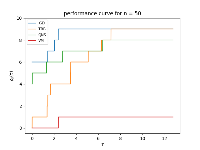
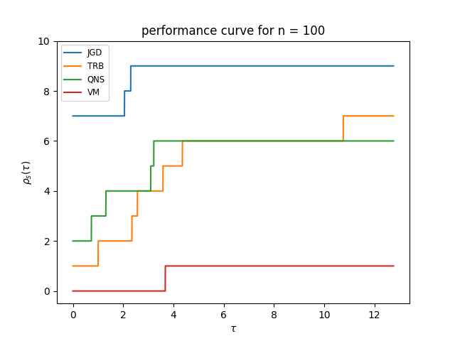
Figure 4: Performance curves of 4 non-smooth optimization methods on solving median size problem instances.

Performance on median-size problem instances All the methods and numerical experiments are implemented in Julia and the automatic differentiation technology has been applied to compute the gradient of a given component function. The computation is performed on a 2.3 GHz 4-core computer with 32 GB RAM. Each job of solving an particular problem instance using a method is managed by a single processor (i.e., no parallel processing). For median-size problem instances ($n=50,100$), we compare the performance of JGD with other three methods TRB, QNS and VM. Figure 4 shows the performance curves of the four methods on solving the 10 test problems for $n=50$ and $n=100$, respectively. The performance curve of a solver is defined as $\rho_{s}(\tau)$ versus $\tau$, where $\tau$ is a changing parameter and $\rho_{s}(\tau)$ is defined as

$$\rho_{s}(\tau):=\frac{\textrm{no. of problems where }\log_{2}(r_{p,s})\leq\tau}{\textrm{total no. of problems}},$$

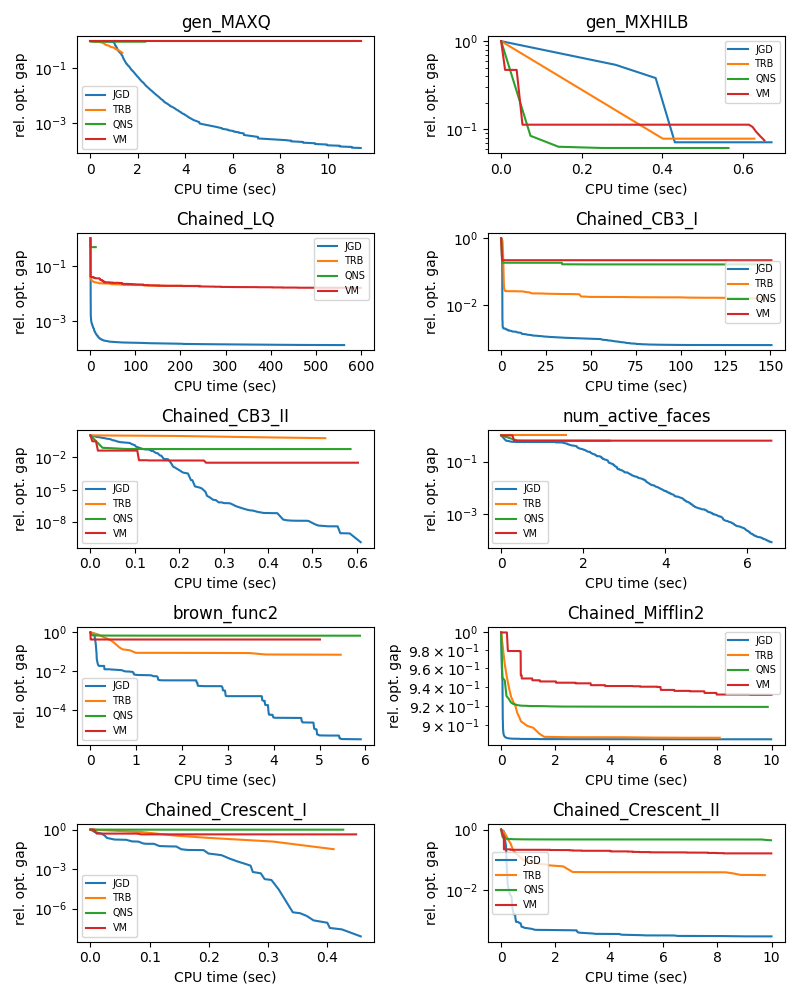
Figure 5: The efficiency of reducing objective values compared for 4 non-smooth optimization methods. The dimension of all problem instances is 100.

where $s$ is the index of the solver, $p$ is the index of problem instance, $r_{p,s}$ is the ratio between the time to solve problem $p$ by solver $s$ over the lowest time required by any of the solvers. The ratio $r_{p,s}$ is set to infinity if solver $s$ cannot terminate with the computational time limit (20 minutes in this case). Table 3 gives the termination times and objective values achieved by every method on each problem instance, and Figure 5 shows the reduction of relative optimality gap (ROG) over time for all objective functions with $n=100$. The plot of performance curves in Figure 4 points out that the JGD is the best of all methods considered which can solve 9 out of 10 instances with Type I and Type II termination criteria for both $n=50$ and $n=100$. From Table 3, the JGD method achieves shorter termination time relative to the other three methods on all instances with only few exceptions, and the quality of solution given by the JGD method is in general magnitudes better than that of the other three methods, which can also be seen from Figure 5.

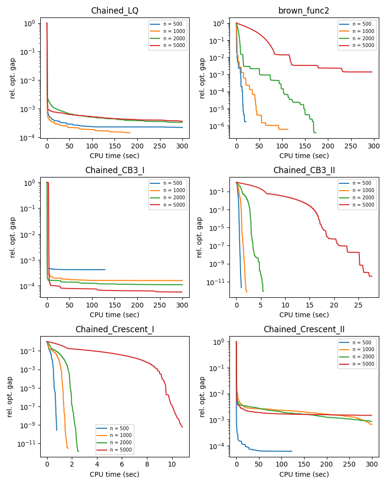
Figure 6: Plot of objective over time generated by the JGD method for selected objective functions and $n=500,1000,2000,5000$.

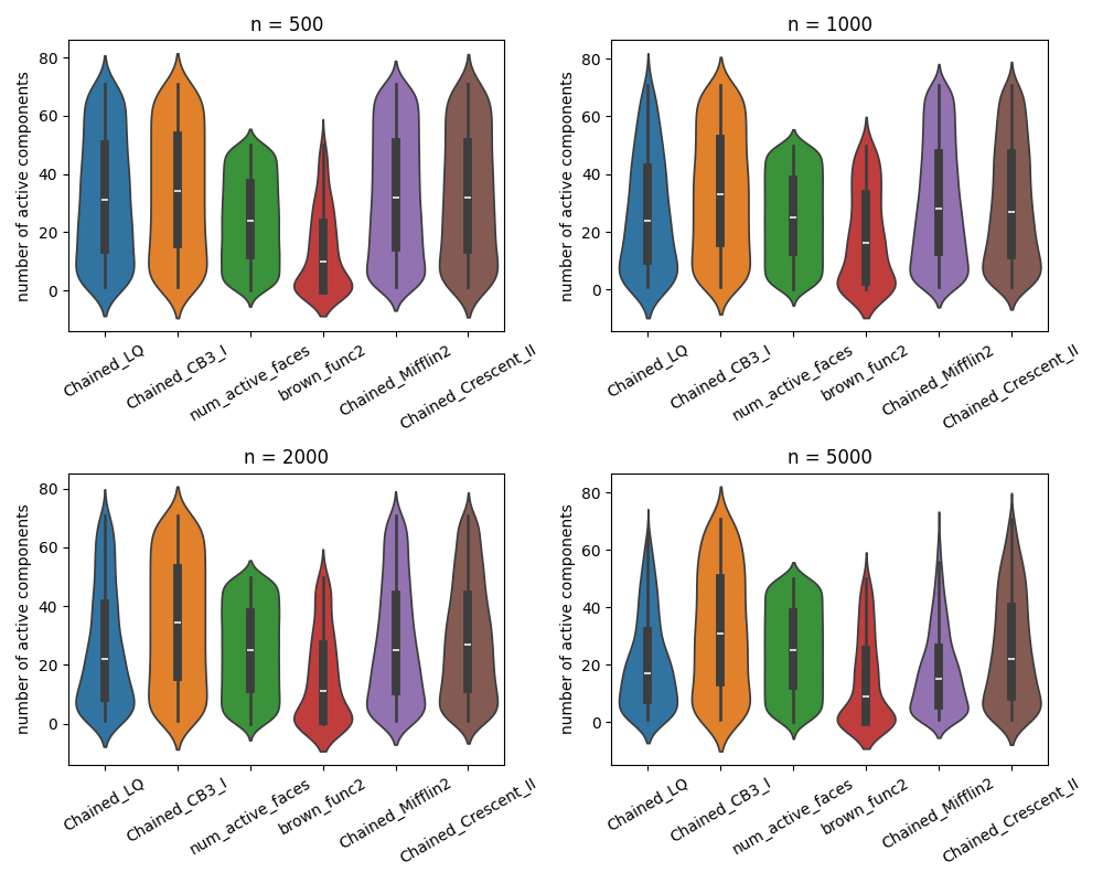
Figure 7: Violin plots of the number of component functions used in computing the joint gradient (referred as the number of active component functions in the figure) in each iteration.

Performance on large problem instances We have noticed that the TRB, QNS and VM method cannot make effectively progress on solving large scale problem instances due to that they need to solve a $n$-dimensional quadratic program with matrix size being $n\times{n}$ and update the matrix in each iteration, which is very computationally expensive for $n\geq 1000$. On the other side, for the JGD method, the dimension of the joint-gradient QP is equal to the number of selected components (i.e., the size of $\mathcal{C}$) which is no greater than 50 as we have set a capacity for $\mathcal{C}$. Furthermore, the joint-gradient QP has a much lower complexity relative to QP’s in the other three methods as it does not require a explicit construction of the matrix. These features make the scale of the joint-gradient QP more robust towards the growth of dimension, and hence more efficient to be solved. In addition to these properties, the joint gradient descent is a more informative search direction by intuition. Therefore, it is not surprising that the JGD has essential advantages in solving large scale problem instances compared to other methods. The performance of using the JGD method to solve large problem instances ($n=500,1000,2000,5000$) is summarized in Table 4 and the relative optimality gap over iterations is visualized in Figure 6. In particular, Table 4 shows that for 15 out of 40 instances, the JGD method can terminate in less than 1 minute. For all instances of gen_MXHILB, Chained_CB3_II and Chained_Crescent_I, the JGD method can solve them within $1\sim 60$ seconds with the relative optimality gap (ROG) from $1\times 10^{-12}$ to $1\times 10^{-4}$. For all instances of Chained_LQ, Chained_CB3_I, brown_func2, Chained_Mifflin2 and Chained_Crescent_II, the JGD method can effectively reduce the ROG to the range of $1\times 10^{-3}\sim 1\times 10^{-6}$. For gen_MAXQ instances, the JGD can reduce ROG to $1\times 10^{-4}\sim 1\times 10^{-3}$ for $n=500,1000$, but it does not perform well on $n=2000,5000$, leaving ROG up to $0.4$. For all instances of num_active_faces, the ROG is up to $0.1\sim 0.4$. Figure 6 shows the efficiency of reducing ROG of 6 selected objective functions for different dimensions. We notice that for Chained_LQ and Chained_CB3_I, the efficiency of ROG reduction is relatively consistent among dimensions. For Chained_CB3_II and Chained_Crescent_I, the ROG can be reduced down to roughly a same level ($<1\times 10^{-}9$) among dimensions, but it takes about 5 time amount of computational time for $n=5000$ compared to $n=500,1000,2000$. For brown_func2, the efficiency very typically depends on the dimension, as the gaps among these curves are very clear. For Chained_Crescent_II, the efficiency for $n=1000,2000,5000$ is very close, while the efficiency for $n=500$ is about 100 times better than the other three problem sizes. The violin plots in Figure 7 show the number $|\mathcal{C}|$ of selected components for joint-gradient calculation and its distribution over iterations. The number $|\mathcal{C}|$ ranges from 1 to 80 as because we have set a capacity for $\mathcal{C}$ and reset $\mathcal{C}$ once its size exceeds the capacity.

5 Concluding Remarks

Potential research directions. The paper demonstrates the power of using component information in designing algorithms for solving practical non-smooth optimization problems from the theoretical and numerical perspectives. Different ways of using the component information in algorithm design and how to integrate this information with empirical rules or machine learning based rules for component selection to further improve the algorithm performance becomes an emerging research direction. In addition, following-up methodology development is needed for various problem settings. For example, suppose some component functions are in a stochastic form, e.g., $f_{\theta}(x)=\mathbb{E}_{\xi}[\psi(x,\xi)]$. Then the evaluation of the function value and gradient of $f_{\theta}$ becomes stochastic. One can imagine that the stochastic ingredient in this problem setting can enrich the algorithm design and the convergence analysis. For another example, suppose the objective function is in a sample-average form: $f(x)=\frac{1}{N}\sum^{N}_{i=1}g(x,\xi_{i})$, and $g(x,\xi)$ is an encodable piecewise-smooth function of $x$. In this case, it is not a good idea to log the component of each $g(x,\xi_{i})$ if the sample size $N$ is a big number, as because the complexity of codes grows linearly with $N$, and the total number of codes grows exponentially with $N$. As a consequence, the importance of a specific component function is diluted. Therefore, how to extract high-level component information and justify it in theoretical and numerical analysis becomes an interesting problem to investigate.

An open problem. In the theorems for linear rate of convergence, i.e., Theorem 3 and Theorem 4, it is assumed that the minimizer is non-degenerate. An open problem is: Is it possible to design an algorithm that can achieve a linear rate of convergence for a general case that the minimizer is possibly degenerate. As an intuition, the analysis for this case can be more intricate and additional validation procedures are needed in the design of such an algorithm.

Algorithm 3 A practical implementation for joint gradient descent method with component information

Parameters: $0<\alpha_{0},\mu_{0},\mu_{\mathrm{dec}}<1$

Data structure: A dictionary dict that maps the code $\theta$ to $[x_{\theta},f_{\theta}(x_{\theta}),\nabla{f}_{\theta}(x_{\theta})]$

Step 1. Initialization: $x\leftarrow{x_{0}}$. Get the code $\theta_{0}$ of active component function at $x_{0}$. Set $\textsc{dict}[\theta_{0}]=[x_{0},f_{\theta_{0}}(x_{0}),\nabla{f}_{\theta_{0}}(x_{0})]$.

Step 2. Component selection: Select a set $\mathcal{C}$ (active set) of codes from dict according to a certain rule based on the proximity of $x_{\theta}$ with respect to the current point $x$.

Step 3. Computation of the joint gradient: Solve the quadratic program

$\min_{\lambda}\left\lVert\sum_{\theta\in\mathcal{C}}\lambda_{\theta}\nabla{f}_{\theta}(x_{\theta})\right\rVert^{2}\;\textrm{s.t. }\sum_{\theta\in\mathcal{C}}\lambda_{\theta}=1$ to determine the joint gradient $d$ and let $\hat{d}=d/\left\lVert d\right\rVert$ be the normalized vector of $d$.

Step 4. Line search: Starting from $\alpha\leftarrow\alpha_{0}$, reduce $\alpha\leftarrow\mu_{\mathrm{dec}}\alpha$ until one finds a step size $\alpha$ such that $[f(x)-f(x-\alpha\hat{d})]/(\alpha\left\lVert d\right\rVert)\geq\mu_{0}$.

Step 5. Component information update: During Step 4, for each test step size $\alpha^{\prime}$, determine the active code $\theta$ at $x-\alpha^{\prime}\hat{d}$. If $\theta\notin\textsc{dict}$ or $\theta\in\textsc{dict}$ but $\|\alpha^{\prime}\hat{d}\|<\left\lVert x_{\theta}-x\right\rVert$, set $x_{\theta}\leftarrow{x}-\alpha^{\prime}\hat{d}$ and set $\textsc{dict}[\theta]=[x_{\theta},f_{\theta}(x_{\theta}),\nabla{f}_{\theta}(x_{\theta})]$.

Step 6. Moving forward and termination check: Set $x\leftarrow{x}-\alpha\hat{d}$. If certain termination criteria are satisfied at $x$, then the algorithm terminates; otherwise, go to Step 2.

Table 2: Test problems [18] and their properties

function name	analytical form
gen_MAXQ	$\max_{1\leq{i}\leq{n}}\;x^{2}_{i}$
gen_MXHILB	$\max_{1\leq{i}\leq{n}}\left|\frac{x_{i}}{i+j-1}\right|$
Chained_LQ	$\sum^{n-1}_{i=1}\max\{-x_{i}-x_{i+1},-x_{i}-x_{i+1}+(x^{2}_{i}+x^{2}_{i+1}-1)\}$
Chained_CB3_I	$\sum^{n-1}_{i=1}\{x^{4}_{i}+x^{2}_{i+1},(2-x_{i})^{2}+(2-x_{i+1})^{2},2e^{-x_{i}+x_{i+1}}\}$
Chained_CB3_II	$\sum^{n-1}_{i=1}\max\{x^{2}_{i}+(x_{i+1}-1)^{2}+x_{i+1}-1,-x^{2}_{i}-(x_{i+1}-1)^{2}+x_{i+1}+1\}$
num_active_faces	$\max_{1\leq{i}\leq{n}}\left\{\log\left|\sum^{n}_{i=1}x_{i}\right|,\log|x_{i}|\right\}$
brown_func2	$\sum^{n-1}_{i=1}\big{(}|x_{i}|^{x^{2}_{i+1}+1}+|x_{i+1}|^{x^{2}_{i}+1}\big{)}$
Chained_Mifflin2	$\sum^{n-1}_{i=1}(-x_{i}+2(x^{2}_{i}+x^{2}_{i+1}-1)+1.75|x^{2}_{i}+x^{2}_{i+1}-1|$
Chained_Crescent_I	$\max\left\{\sum^{n-1}_{i=1}(x^{2}_{i}+(x_{i+1}-1)^{2}+x_{i+1}-1),\sum^{n-1}_{i=1}(-x^{2}_{i}-(x_{i+1}-1)^{2}+x_{i+1}+1)\right\}$
Chained_Crescent_II	$\sum^{n-1}_{i=1}\max\{x^{2}_{i}+(x_{i+1}-1)^{2}+x_{i+1}-1,-x^{2}_{i}-(x_{i+1}-1)^{2}+x_{i+1}+1\}$

function name	optimal objective	Convexity	uniform domain
gen_MAXQ	0.0	$+$	$+$
gen_MXHILB	0.0	$+$	$+$
Chained_LQ	$-\sqrt{2}(n-1)$	$+$	$+$
Chained_CB3_I	$2(n-1)$	$+$	$+$
Chained_CB3_II	$2(n-1)$	$+$	$+$
num_active_faces	0.0	$-$	$-$
brown_func2	0.0	$-$	$-$
Chained_Mifflin2	unclear∗	$-$	$+$
Chained_Crescent_I	0.0	$-$	$+$
Chained_Crescent_II	0.0	$-$	$+$

^∗$f(x^{*})\approx-6.51$ for $n=10$, $f(x^{*})\approx-70.15$ for $n=100$, and $f(x^{*})\approx-706.55$ for $n=1000$.

Table 3: Performance of non-smooth optimization methods on median-size problem instances

function name	dim	time(JGD)	obj(JGD)	time(TRB)	obj(TRB)	time(QN)	obj(QN)	time(VM)	obj(VM)
gen_MAXQ	50	3.47	3.011E-03	3.49	2.305E-01	-	9.492E-01	-	9.357E-01
gen_MAXQ	100	11.39	1.224E-04	13.70	2.384E-01	2.31	9.553E-01	-	9.606E-01
gen_MXHILB	50	1.43	1.112E-04	15.91	2.100E-02	1.45	1.120E-01	7.45	1.552E-02
gen_MXHILB	100	0.67	9.929E-02	3.41	1.091E-01	1.66	8.559E-02	8.57	5.592E-02
Chained_LQ	50	-	2.483E-03	27.07	2.837E+00	10.08	3.712E+01	-	5.902E-01
Chained_LQ	100	-	2.017E-02	243.54	2.810E+00	11.90	7.118E+01	-	2.373E+00
Chained_CB3_I	50	48.17	1.784E-05	613.86	7.054E+00	18.08	6.998E+01	-	2.908E+01
Chained_CB3_I	100	150.65	4.408E-01	-	2.096E+00	-	1.122E+02	-	1.499E+02
Chained_CB3_II	50	1.77	1.018E-06	250.54	4.028E+00	4.39	2.444E+01	-	7.854E-01
Chained_CB3_II	100	0.61	9.966E-08	-	1.493E+00	5.20	3.682E+01	-	1.930E+00
num_active_faces	50	15.57	4.413E-05	43.36	4.546E-01	3.84	5.558E-01	-	4.166E-01
num_active_faces	100	6.59	9.375E-05	1.59	1.094E+00	2.64	6.860E-01	-	5.082E-01
brown_func2	50	9.91	3.279E-04	-	1.438E+00	832.63	5.375E-03	82.58	4.326E+00
brown_func2	100	5.90	2.516E-04	-	1.278E+00	-	3.345E+00	24.01	3.028E+01
Chained_Mifflin2	50	69.44	-3.476E+01	34.39	-3.348E+01	13.39	-2.240E+01	-	-2.957E+01
Chained_Mifflin2	100	44.67	-7.000E+01	89.64	-6.917E+01	-	-4.892E+01	-	-5.408E+01
Chained_Crescent_I	50	0.44	2.869E-08	34.62	2.891E+00	3.01	3.592E+01	-	3.857E+00
Chained_Crescent_I	100	0.46	4.954E-07	789.75	7.449E-01	4.24	6.288E+01	-	1.408E+00
Chained_Crescent_II	50	21.10	1.882E-05	66.26	1.785E+00	-	4.817E+00	-	1.725E+00
Chained_Crescent_II	100	19.67	2.881E-02	235.80	2.485E+00	-	3.706E+01	-	6.338E+00

Table 4: Performance of the joint gradient descent method on solving large-size problem instances. For columns of objective value checkpoints, the symbol ‘-’ indicates that the termination time is shorter than that checkpoint time.

function name	dim	obj(init)	term. time (sec)	obj(final)	obj(1min)	obj(5min)	obj(10min)	components
gen_MAXQ	500	9.950E-01	158.69	2.228E-04	9.525E-03	-	-	497
gen_MAXQ	1000	9.995E-01	570.74	3.444E-04	2.460E-01	4.802E-03	-	990
gen_MAXQ	2000	9.995E-01	1200.02	1.876E-02	5.565E-01	1.645E-01	6.840E-02	1736
gen_MAXQ	5000	9.995E-01	1201.13	4.829E-01	8.733E-01	7.137E-01	6.128E-01	1503
gen_MXHILB	500	1.328E+00	0.77	4.655E-04	-	-	-	44
gen_MXHILB	1000	1.343E+00	3.00	3.334E-04	-	-	-	54
gen_MXHILB	2000	1.318E+00	9.16	4.143E-04	-	-	-	110
gen_MXHILB	5000	1.316E+00	57.78	2.234E-04	-	-	-	113
Chained_LQ	500	7.141E+02	4729.99	1.534E-01	1.907E-01	1.570E-01	1.534E-01	2769
Chained_LQ	1000	1.468E+03	12646.27	2.095E-01	3.157E-01	2.096E-01	2.096E-01	1222
Chained_LQ	2000	2.868E+03	1200.26	5.463E-01	1.755E+00	9.489E-01	6.637E-01	3861
Chained_LQ	5000	7.260E+03	1201.88	1.732E+00	4.344E+00	2.632E+00	2.195E+00	1933
Chained_CB3_I	500	3.286E+03	128.51	1.390E+00	1.392E+00	-	-	2082
Chained_CB3_I	1000	6.723E+03	348.09	1.083E+00	1.162E+00	1.083E+00	-	3103
Chained_CB3_I	2000	1.317E+04	727.93	1.446E+00	1.833E+00	1.459E+00	1.447E+00	2925
Chained_CB3_I	5000	3.323E+04	1200.61	1.557E+00	2.616E+00	1.928E+00	1.675E+00	1535
Chained_CB3_II	500	3.259E+03	1.05	7.715E-09	-	-	-	3
Chained_CB3_II	1000	6.667E+03	2.19	4.829E-09	-	-	-	3
Chained_CB3_II	2000	1.306E+04	5.52	1.121E-08	-	-	-	3
Chained_CB3_II	5000	3.298E+04	27.75	1.334E-06	-	-	-	3
num_active_faces	500	2.286E+00	39.98	3.499E-01	-	-	-	1215
num_active_faces	1000	1.024E+00	58.49	4.976E-01	-	-	-	818
num_active_faces	2000	3.603E+00	105.31	5.999E-01	6.003E-01	-	-	604
num_active_faces	5000	3.636E+00	888.69	6.511E-01	6.946E-01	6.915E-01	6.865E-01	729
brown_func2	500	4.415E+02	20.89	7.558E-04	-	-	-	2055
brown_func2	1000	8.693E+02	112.39	5.314E-04	1.284E-03	-	-	2930
brown_func2	2000	1.753E+03	173.31	6.742E-04	1.628E+00	-	-	2741
brown_func2	5000	4.314E+03	909.55	2.513E-03	6.112E+02	5.994E+00	9.356E-02	2847
Chained_Mifflin2	500	4.378E+01	436.39	-3.524E+02	-3.519E+02	-3.524E+02	-	8833
Chained_Mifflin2	1000	1.024E+02	1200.21	-7.052E+02	-7.025E+02	-7.049E+02	-7.052E+02	13750
Chained_Mifflin2	2000	1.977E+02	1200.07	-1.411E+03	-1.408E+03	-1.410E+03	-1.411E+03	6668
Chained_Mifflin2	5000	4.594E+02	1201.23	-3.527E+03	-3.514E+03	-3.522E+03	-3.525E+03	4152
Chained_Crescent_I	500	3.271E+02	0.78	8.950E-08	-	-	-	2
Chained_Crescent_I	1000	6.641E+02	1.70	2.128E-09	-	-	-	2
Chained_Crescent_I	2000	1.311E+03	2.54	1.880E-09	-	-	-	2
Chained_Crescent_I	5000	3.244E+03	10.83	1.826E-06	-	-	-	2
Chained_Crescent_II	500	5.312E+02	122.62	3.236E-02	3.302E-02	-	-	2479
Chained_Crescent_II	1000	1.052E+03	649.33	1.654E-01	2.741E+00	6.928E-01	1.655E-01	7748
Chained_Crescent_II	2000	2.117E+03	1200.09	8.867E-01	5.277E+00	1.812E+00	1.027E+00	7318
Chained_Crescent_II	5000	5.238E+03	1201.34	4.886E+00	9.379E+00	7.649E+00	6.221E+00	2968

Appendix A Omitted proofs

proof of Proposition 1.

(a) Consider the following quadratic program:

$$\min_{\lambda}\;\left\lVert\sum^{k}_{i=1}\lambda_{i}a_{i}\right\rVert^{2}\quad\textrm{s.t. }\;\sum^{k}_{i=1}\lambda_{i}=1,$$ (A.1)

which can be written equivalently as: $\min_{\lambda}\;\left\lVert A\lambda\right\rVert^{2}\quad\textrm{s.t. }\;e^{\top}\lambda=1$. Using the Lagrangian multiplier method, one can verify that the optimal solution $\lambda^{*}$ of the above quadratic program is

$$\lambda^{*}=\frac{1}{e^{\top}(A^{\top}A)^{-1}e}\cdot(A^{\top}A)^{-1}e,$$ (A.2)

and we have $d^{*}=A\lambda^{*}$. Furthermore, we have

$$[\left\langle a_{1},d^{*}\right\rangle,\left\langle a_{2},d^{*}\right\rangle,\ldots,\left\langle a_{k},d^{*}\right\rangle]^{\top}=A^{\top}d^{*}=\frac{e}{e^{\top}(A^{\top}A)^{-1}e},$$

which implies that

$$\left\langle a_{i},d^{*}\right\rangle=\frac{1}{e^{\top}(A^{\top}A)^{-1}e}\quad\forall{i\in[k]}.$$

It means that moving along the direction $d_{i}$, each $f_{i}$ has the same amount of increment.

(b) We compute the decrement value of $f$ along any normalized direction $-\hat{d}$ at $x_{0}$, where $\|\hat{d}\|=1$. First, $\hat{d}$ can be uniquely decomposed as $\hat{d}=d^{\prime}+\alpha\hat{d}^{*}$ for some $\alpha\leq 1$ such that $\langle d^{\prime},\hat{d}^{*}\rangle=0$, where $\hat{d}^{*}=d^{*}/\left\lVert d^{*}\right\rVert$. The decrement of $f$ along $-\hat{d}$ with step-size $\delta$ can be computed as

$$f(x_{0})-f(x_{0}-\delta\hat{d}) =\max\{a^{\top}_{i}x_{0}+b_{i}:\forall i\in[k]\}-\max\{a^{\top}_{i}(x_{0}-\delta\hat{d})+b_{i}:\forall i\in[k]\}$$

$$=f(x_{0})-\left(f(x_{0})-\min\{\delta a^{\top}_{i}\hat{d}:\forall i\in[k]\}\right)$$

$$=\min\{\delta a^{\top}_{i}\hat{d}:\forall i\in[k]\}.$$

Note that we have

$$\langle a_{i},\hat{d}\rangle =\alpha\langle a_{i},\hat{d}^{*}\rangle+\langle a_{i},d^{\prime}\rangle$$

$$=\alpha\langle a_{i},\hat{d}^{*}\rangle+\langle a_{i}-d^{*},d^{\prime}\rangle+\langle d^{*},d^{\prime}\rangle$$

$$=\alpha\left\lVert d^{*}\right\rVert+\left\langle a_{i}-d^{*},d^{\prime}\right\rangle.$$

Since we have $\sum^{k}_{i=1}\lambda^{*}_{i}\left\langle a_{i}-d^{*},d^{\prime}\right\rangle=0$ by the property of $d^{*}$ and $\lambda^{*}$, there exists an index $j$ such that $\left\langle a_{j}-d^{*},d^{\prime}\right\rangle\leq 0$ given that $\lambda^{*}\geq 0$. Using this property, we further compute

$$f(x_{0})-f(x_{0}-\delta\hat{d}) =\delta\alpha\left\lVert d^{*}\right\rVert+\min\{\delta\left\langle a_{i}-d^{*},d^{\prime}\right\rangle:\forall i\in[k]\}$$

$$\leq\delta\alpha\left\lVert d^{*}\right\rVert\leq\delta\left\lVert d^{*}\right\rVert,$$

where the equality holds if $\alpha=1$, i.e., $\hat{d}=\hat{d}^{*}$. This indicates that indeed, $-d^{*}$ is the steepest descent direction of $f$ at $x_{0}$. ∎

proof of Proposition 2.

Let $u=\sum_{i\in\mathcal{I}}\lambda^{*}_{i}v_{i}$ and consider the following two-variate problem for any $i\in\mathcal{I}^{\prime}$

$$\min_{\alpha_{1},\alpha_{2}}\left\lVert\alpha_{1}u+\alpha_{2}v_{i}\right\rVert^{2}\quad\mathrm{s.t.}\;\alpha_{1}+\alpha_{2}=1,\;\alpha_{1},\alpha_{2}\geq 0.$$ (A.3)

By the optimality condition of (2.5), the above problem must have an optimal solution $[\alpha^{*}_{1},\alpha^{*}_{2}]=[1,0]$, otherwise $\lambda^{*}$ cannot be the optimal solution of (2.5). The Lagrangian of (A.3) is given by

$$L(\alpha,\beta)=\left\lVert\alpha_{1}u+\alpha_{2}v_{i}\right\rVert^{2}+\beta(\alpha_{1}+\alpha_{2}-1)-\tau_{1}\alpha_{1}-\tau_{2}\alpha_{2}.$$

The KKT conditions of (A.3) read as

$$2\alpha_{1}\left\lVert u\right\rVert^{2}+2\alpha_{2}\left\langle u,v_{i}\right\rangle+\beta-\tau_{1}=0,$$

$$2\alpha_{2}\left\lVert v_{i}\right\rVert^{2}+2\alpha_{1}\left\langle u,v_{i}\right\rangle+\beta-\tau_{2}=0,$$

$$\alpha_{1}+\alpha_{2}=1,\;\alpha_{1}\tau_{1}=0,\;\alpha_{2}\tau_{2}=0,\;\alpha_{1},\alpha_{2},\tau_{1},\tau_{2}\geq 0,$$

and they lead to the following condition after eliminating $\alpha_{1}$ and $\beta$

$$(\left\lVert u\right\rVert-\left\lVert v_{i}\right\rVert)^{2}\alpha_{2}+\frac{\tau_{1}-\tau_{2}}{2}=\left\lVert u\right\rVert^{2}-\left\langle u,v_{i}\right\rangle.$$

Since $[\alpha^{*}_{1},\alpha^{*}_{2}]=[1,0]$ is a solution of the KKT system, the complementary slackness condition implies that $\tau_{1}=0$. Substituting $\alpha^{*}_{2}=0$ and $\tau_{1}=0$ into the above equation gives

$$\left\lVert u\right\rVert^{2}-\left\langle u,v_{i}\right\rangle=-\frac{\tau_{2}}{2}\leq 0,$$

which concludes the proof. ∎

Observation 2.

For any continuous function $g$, if $x^{*}$ is the unique local minimizer of $g$ the set $U(v):=\{x:g(x)\leq{v}\}$ for $v\geq{g(x^{*})}$ is a connected closed set containing $x^{*}$

Proof.

Suppose there exists a value $v\geq{g(x^{*})}$ such that $U(v)$ is a closed set consisting of multiple disjointed (closed) subsets $V_{1},\ldots,V_{k}$ ($k\geq 2$). Suppose $x^{*}\in{V}_{1}$. By definition of the level sets, there must exist a local minimizer in $V_{2}$ which is different from $x^{*}$. This contradicts to that $x^{*}$ is the unique local minimizer of $g$. ∎

Proposition 10.

For any $x_{0}\in X$, the function $v(x)=\left\lVert\mathrm{vec(}\mathrm{QP}\textrm{-}{x}\textrm{-}{\mathcal{C}}\mathrm{)}\right\rVert$ is continuous at $x_{0}$ in a neighborhood $B$ of $x_{0}$ satisfying $\mathcal{C}\subseteq\widetilde{\mathcal{M}}(x)$ for every $x\in{B}$.

Proof.

By definition $\mathrm{vec(}\mathrm{QP}\textrm{-}{x}\textrm{-}{\mathcal{C}}\mathrm{)}$ is an optimal vector of the following QP:

$$\min_{\lambda}\;\left\lVert\sum_{\theta\in\mathcal{C}}\lambda_{\theta}\nabla{f_{\theta}(x)}\right\rVert\;\textrm{s.t. }\sum_{\theta\in\mathcal{C}}\lambda_{\theta}=1,\;\lambda\geq 0.$$ (A.4)

Let $\lambda^{*}$ be an optimal solution at $x_{0}$ of the above QP. The continuity of $v(x)$ at $x_{0}$ follows from the fact that $\nabla{f_{\theta}}$ is continuous at $x_{0}$ for $\theta\in\mathcal{C}$. ∎

References

• [1] Felipe Atenas, Claudia Sagastizábal, Paulo J. S. Silva, and Mikhail Solodov. A unified analysis of descent sequences in weakly convex optimization, including convergence rates for bundle methods. SIAM Journal on Optimization, 33(1):89–115, 2023.
• [2] Adil Bagirov, Napsu Karmitsa, and Marko M. Mäkelä. Bundle methods. In Introduction to Nonsmooth Optimization, chapter 12, pages 305–310. Springer International Publishing, Switzerland, 2014.
• [3] James V. Burke, Adrian S. Lewis, and Michael L. Overton. A robust gradient sampling algorithm for nonsmooth, nonconvex optimization. SIAM Journal on Optimization, 15(3):751–779, 2005.
• [4] Vasileios Charisopoulos and Damek Davis. A superlinearly convergent subgradient method for sharp semismooth problems. Mathematics of Operations Research, in press.
• [5] Ying Cui and Jong-Shi Pang. Modern nonconvex nondifferentiable optimization. MOS-SIAM Series on Optimization. Society for Industrial and Applied Mathematics, Philadelphia, PA, 2021.
• [6] Frank E. Curtis and Minhan Li. Gradient sampling methods with inexact subproblem solves and gradient aggregation. arXiv, 2021.
• [7] Frank E. Curtis and Xiaocun Que. A quasi-newton algorithm for nonconvex, nonsmooth optimization with global convergence guarantees. Mathematical Programming Computation, 7:399–428, 2015.
• [8] Minh N. Dao. Bundle method for nonconvex nonsmooth constrained optimization. Journal of Convex Analysis, 22:1061–1090, 2015.
• [9] Minh N. Dao, Joachim Gwinner, Dominikus Noll, and Nina Ovcharova. Nonconvex bundle method with application to a delamination problem. Computational Optimization and Applications, 65:173–203, 2016.
• [10] Mateo Díaz and Benjamin Grimmer. Optimal convergence rates for the proximal bundle method. SIAM Journal on Optimization, 33:424–454, 2023.
• [11] Yu Du and Andrzej Ruszczyński. Rate of convergence of the bundle method. Journal of Optimization Theory and Applications, 173:908–922, 2017.
• [12] Sabrina Fiege, Andrea Walther, and Andreas Griewank. An algorithm for nonsmooth optimization by successive piecewise linearization. Mathematical Programming, 177:343–370, 2019.
• [13] Sabrina Fiege, Andrea Walther, Kshitij Kulshreshtha, and Andreas Griewank. Algorithmic differentiation for piecewise smooth functions: a case study for robust optimization. Optimization Methods and Software, 33(4-6):1073–1088, 2018.
• [14] Andreas Griewank. On stable piecewise linearization and generalized algorithmic differentiation. Optimization Methods and Software, 28:1139–1178, 2013.
• [15] Andreas Griewank and Andrea Walther. First- and second-order optimality conditions for piecewise smooth objective functions. Optimization Methods and Software, 31(5):904–930, 2016.
• [16] Andreas Griewank and Andrea Walther. Relaxing kink qualifications and proving convergence rates in piecewise smooth optimization. SIAM Journal on Optimization, 29(1):262–289, 2019.
• [17] Andreas Griewank, Andrea Walther, Sabrina Fiege, and Torsten Bosse. On Lipschitz optimization based on gray-box piecewise linearization. Mathematical Programming, 158:383–415, 2016.
• [18] M. Haarala, K. Miettinen, and M. M. Makela. New limited memory bundle method for large-scale nonsmooth optimization. Optimization Methods and Software, 19(6):673–692, 2004.
• [19] X. Y. Han and Adrian S. Lewis. Survey descent: a multipoint generalization of gradient descent for nonsmooth optimization. SIAM Journal on Optimization, 33(1):36–62, 2023.
• [20] W. Hare, C. Sagastizábal, and M. Solodov. A proximal bundle method for nonsmooth nonconvex functions with inexact information. Computational Optimization and Applications, 63:1–28, 2015.
• [21] Warren Hare and Claudia Sagastizábal. A redistributed proximal bundle method for nonconvex optimization. SIAM Journal on Optimization, 20(5):2442–2473, 2010.
• [22] Michael Hintermüller. A proximal bundle method based on approximate subgradients. Computational Optimization and Applications, 20:245–266, 2001.
• [23] Krzysztof C. Kiwiel. Restricted step and Levenberg-Marquardt techniques in proximal bundle methods for nonconvex nondifferentiable optimization. SIAM Journal on Optimization, 6(1):227–249, 1996.
• [24] Krzysztof C. Kiwiel. A proximal bundle method with approximate subgradient linearization. SIAM Journal on Optimization, 16(4):1007–1023, 2006.
• [25] Krzysztof C. Kiwiel. Convergence of the gradient sampling algorithm for nonsmooth nonconvex optimization. SIAM Journal on Optimization, 18(2):379–388, 2007.
• [26] C. Lemaréchal. Bundle methods in nonsmooth optimization. In C. Lemaréchal and R. Mifflin, editors, Nonsmooth Optimization, pages 79–102, Laxenburg, 1977. Pergamon Press, Oxford.
• [27] Adrian S. Lewis and Michael L. Overton. Nonsmooth optimization via quasi-Newton methods. Mathematical Programming, 141:135–163, 2013.
• [28] Ladislav Lukšan and Jan Vlček. A bundle-Newton method for nonsmooth unconstrained minimization. Mathematical Programming, 83:373–391, 1998.
• [29] Jian Lv, Li-Ping Pang, and Fan-Yun Meng. A proximal bundle method for constrained nonsmooth nonconvex optimization with inexact information. Journal of Global Optimization, 70:517–549, 2018.
• [30] Morteza Maleknia and Mostafa Shamsi. A quasi-Newton proximal bundle method using gradient sampling technique for minimizing nonsmooth convex functions. Optimization Methods and Software, 37(4):1415–1446, 2022.
• [31] Robert Mifflin, Defeng Sun, and Liqun Qi. Quasi-Newton bundle-type methods for nondifferentiable convex optimization. SIAM Journal on Optimization, 8(2):583–603, 1998.
• [32] N. Hoseini Monjezi and S. Nobakhtian. Convergence of the proximal bundle algorithm for nonsmooth nonconvex optimization problems. Optimization Letter, 16:1495–1511, 2022.
• [33] Najmeh H. Monjezi. A bundle trust region algorithm for minimizing locally Lipschitz functions. SIAM Journal on Optimization, 33(1):319–337, 2023.
• [34] Najmeh H. Monjezi and S. Nobakhtian. A filter proximal bundle method for nonsmooth nonconvex constrained optimization. Journal of Global Optimization, 79:1–37, 2021.
• [35] Najmeh Hoseini Monjezi and S. Nobakhtian. A new infeasible proximal bundle algorithm for nonsmooth nonconvex constrained optimization. Computational Optimization and Applications, 74:443–480, 2019.
• [36] Claudia Sagastizábal. Composite proximal bundle method. Mathematical Programming, 140:189–233, 2013.
• [37] J. Vlcek and L. Luksan. Globally convergent variable metric method for nonconvex nondifferentiable unconstrained minimization. Journal of Optimization Theory and Applications, 111(2):407–430, 2001.
• [38] Andreas Wächter and Lorenz T. Biegler. On the implementation of an interior-point filter line-search algorithm for large-scale nonlinear programming. Mathematical Programming, 106(6):25–57, 2006.