Reconstructing Cosmic History: JWST-Extended Mapping of the Hubble Flow from z$\sim$0 to z$\sim$7.5 with HII Galaxies

Abstract

Over twenty years ago, Type Ia Supernovae (SNIa) [1, 2] observations revealed an accelerating Universe expansion, suggesting a significant dark energy presence, often modelled as a cosmological constant, $\Lambda$. Despite its pivotal role in cosmology, the standard $\Lambda$CDM model remains largely underexplored in the redshift range between distant SNIa and the Cosmic Microwave Background (CMB). This study harnesses the James Webb Space Telescope’s advanced capabilities to extend the Hubble flow mapping across an unprecedented redshift range, from $z\approx 0$ to $z\approx 7.5$. Utilising a dataset of 231 HII galaxies and extragalactic HII regions, we employ the $\text{L}-\sigma$ relation, correlating the luminosity of Balmer lines with their velocity dispersion, to define a competitive technique for measuring cosmic distances. This approach maps the Universe’s expansion over more than 12 billion years, covering 95% of its age. Our analysis, using Bayesian inference, constrains the parameter space $\{h,\Omega_{m},w_{0}\}=\{0.731\pm 0.039,0.302^{+0.12}_{-0.069},-1.01^{+0.52}_{-0.29}\}$ (statistical) for a flat Universe. These results provide new insights into cosmic evolution and suggest uniformity in the photo-kinematical properties of young massive ionizing clusters in giant HII regions and HII galaxies across most of the Universe’s history.

Introduction

Observational campaigns targeting high redshift ($z$) cosmological tracers are underway to refine our understanding of the Dark Energy (DE) Equation of State (EoS). A central objective is to ascertain if the $w$ parameter, which determines the relationship between pressure $p$ and the mass-energy density $\rho c^{2}$ within the DE EoS, undergoes evolution over cosmic time [3, 4]. By rigorously constraining cosmological parameters and cross-validating findings via diverse, independent methodologies, we aim to produce a more accurate and resilient cosmological framework.

H ii galaxies (HIIGs) represent intense and compact star formation episodes predominantly found in dwarf irregular galaxies, where they significantly contribute to the overall luminosity. HIIGs are spectroscopically selected as the star forming systems with the largest equivalent width of their Balmer emission lines ($EW(\mathrm{H}\beta)>50$ Å). This selection criterion guarantees that HIIGs are the youngest systems ($\lesssim$ 5 Myr) that can be studied in detail. Similarly, giant extragalactic H ii regions (GEHRs) are associated with vigorous star formation, but they are typically situated in the outer disks of late-type galaxies. Notably, the rest-frame optical spectra of both GEHRs and HIIGs are virtually indistinguishable from each other, marked by pronounced emission lines. These lines arise from gas ionisation events triggered by a massive Young Stellar Cluster (YSC) or an ensemble of such clusters, often referred to as a Super Star Cluster (SSC) [5, 6, 7, 8, 9].

The pronounced emission lines in the rest-frame optical spectra of GEHRs and HIIGs position them as potent probes for investigating young star formation at high-$z$. Utilising instruments such as NIRSpec [10] onboard the JWST [11], it becomes feasible to delve into these regions up to $z\sim 6.5$ via the H$\alpha$ emission line or even up to $z\sim 9$ using the H$\beta$ and [OIII]$\lambda\lambda 4959,5007$ Å emission lines. Consequently, this allows for the observation of luminous HIIGs, tracing back to the epoch of reionisation.

Multiple studies have proven that both HIIGs and GEHRs exhibit a correlation between their Balmer lines luminosity, e.g. $L(H\beta)$, and the ionised gas velocity dispersion, $\sigma$, traced by these emission lines. This correlation, known as the $\text{L}-\sigma$ relation [12, 13, 14, 9], serves as a powerful cosmological distance indicator [15, 16, 17, 18]. Consequently, the $\text{L}-\sigma$ relation offers a unique avenue for employing this distance estimator to study the Hubble flow across a vast $z$ range.

In this work we present the use of the $\text{L}-\sigma$ relation of GEHRs and HIIGs as a cosmological tracer up to $z\sim 7.5$ and the resulting constraints to cosmological parameters. Our analysis demonstrates the efficacy of GEHRs and HIIGs in tracing the evolution of the Universe, offering insights into the dynamics of the cosmic expansion and the distribution of matter across a significant portion of cosmic history. The results presented herein, unprecedented in redshift dynamical range; from 0 to $\sim$ 7.5, contribute to the ongoing efforts to constrain cosmological models with greater precision, utilising the unique properties of these astrophysical objects.

Results

Here, using a dataset of 231 GEHRs and HIIGs, we have derived constraints applicable to various cosmological models, using the MultiNest Bayesian inference algorithm [19, 20, 21], to maximise the likelihood function and get constraints to the different combinations of nuisance and cosmological parameters. For our analysis, we adopted uniform, non-informative priors across all parameters, ensuring an unbiased estimation. The derived constraints are detailed in Table 1. This table presents the marginalised best-fit values alongside their corresponding $1\sigma$ uncertainties for each parameter. Note that parameters enclosed in parentheses were held constant during the analysis, as they are not free parameters in the respective cosmological models under consideration.

Our main focus consists on constraining a generalised parameter space, denoted as $\theta=\{\alpha,\beta,h,\Omega_{m},w_{0},w_{a}\}$. Here, $\theta_{n}=\{\alpha,\beta\}$ represents nuisance parameters, specifically characterising the $\text{L}-\sigma$ relation for GEHRs and HIIGs, where $\alpha$ is the intercept and $\beta$ the slope of this relation. The remainder of the parameter space pertains to distinct cosmological models. For the flat $\Lambda$CDM model, the parameters are defined as $\theta_{c}=\{h,\Omega_{m},-1,0\}$, indicating that we constrain the reduced Hubble constant $h=H_{0}/(100\ \mathrm{km\ s^{-1}\ Mpc^{-1}})$ and the total matter density parameter, $\Omega_{m}$, while maintaining constant the first two DE EoS parameters at $w_{0}=-1$ and $w_{a}=0$. This specific setting aligns with a cosmological constant ($\Lambda$). Extending the constraints to include the value of $w_{0}$ allows for an evolving DE EoS, characteristic of models akin to quintessence [22, 4]. Lastly, incorporating a constraint on $w_{a}$ aligns with the Chevallier-Polarski-Linder (CPL) model, as delineated in the seminal works [23, 24, 25].

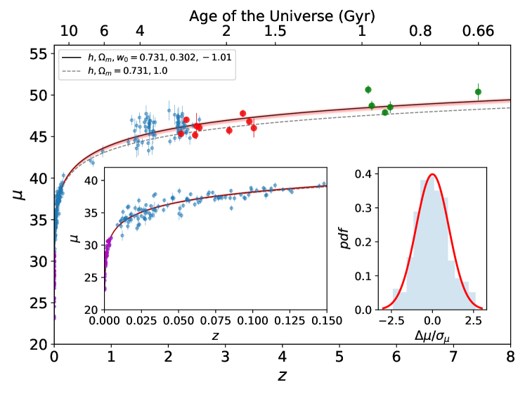
Figure 1: Hubble diagram for GEHRs and HIIGs, here $z$ is the redshift and $\mu$ is the distance modulus. In magenta we present the ‘anchor’ sample of 36 GEHRs which have been analysed in [26], in blue we present the full sample of 181 HIIGs which have been analysed in [18], while in red we present the 9 new HIIGs from [27] and in green the 5 new HIIGs studied with JWST by [28]. The black line is the cosmological model that best fits the data with the red shaded area representing the 1$\sigma$ uncertainties to the model, while the grey dashed line is a flat cosmological model without dark energy. The inset at the left shows a close-up of the Hubble diagram for $z\leq 0.15$. The inset at the right presents the pulls probability density function (pdf) of the entire sample of GEHRs and HIIGs and the red line shows the best Gaussian fit to the pdf.

In Figure 1 we present the Hubble diagram for GEHRs and HIIGs. In magenta we plot the ‘anchor’ sample of 36 GEHRs which have been analysed in [26], in blue we present the full sample of 181 HIIGs, analysed in [18], while in red we show the 9 new HIIGs from [27] and in green 5 HIIGs newly observed with JWST from [28]. The black line is the cosmological model that best fits the data with the red shaded area representing the 1$\sigma$ uncertainties to the model, while the gray dashed line is a flat cosmological model without dark energy. The inset at the left shows a close-up of the Hubble diagram for $z\leq 0.15$. The inset at the right presents the normalised residuals (or ‘pulls’) distribution of the entire sample of GEHRs and HIIGs and the red line shows the best Gaussian fit to the distribution.

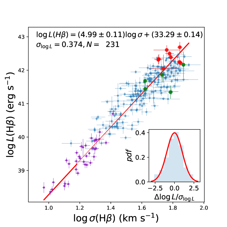
Figure 2: The $L-\sigma$ relation of GEHRs and HIIGs. The data points follow the same colour code for the different samples as in the previous figure. The red line shows the best linear fit to the data, including the uncertainties in both axis. At the top of the figure we present the values of the slope and intercept of the best fit including their uncertainties. We also show the standard deviation of the $\log$ L around the best fit and the total number of objects in the sample. The inset shows the pulls distribution of the entire sample of GEHRs and HIIGs and the red line shows the best Gaussian fit to the distribution.

In Figure 2 we showcase the $\text{L}-\sigma$ relation for GEHRs and HIIGs. The data encompass four distinct groups, as explained above. The red line in the diagram represents the best linear fit to the data, accounting for uncertainties in both luminosity and velocity dispersion axes. Atop the figure we present the slope and intercept values of this best-fit line, along with their respective uncertainties. Additionally, we quantify the standard deviation of the logarithm of the luminosity ($\log L$) around the best fit, providing a measure of the scatter in the data. The total number of objects in the combined sample is also noted, offering a sense of the statistical robustness of the analysis. The inset in the figure displays the normalised residuals (or ‘pulls’) distribution for the entire dataset of GEHRs and HIIGs. The best Gaussian fit to these residuals is shown by the red line showing that the pulls distribution follows closely the fit. This comprehensive analysis of the $\text{L}-\sigma$ relation across a diverse set of GEHRs and HIIGs, including the latest JWST data, provides valuable insights into the underlying physics of these galaxies and contributes significantly to our understanding of galactic dynamics and star formation processes.

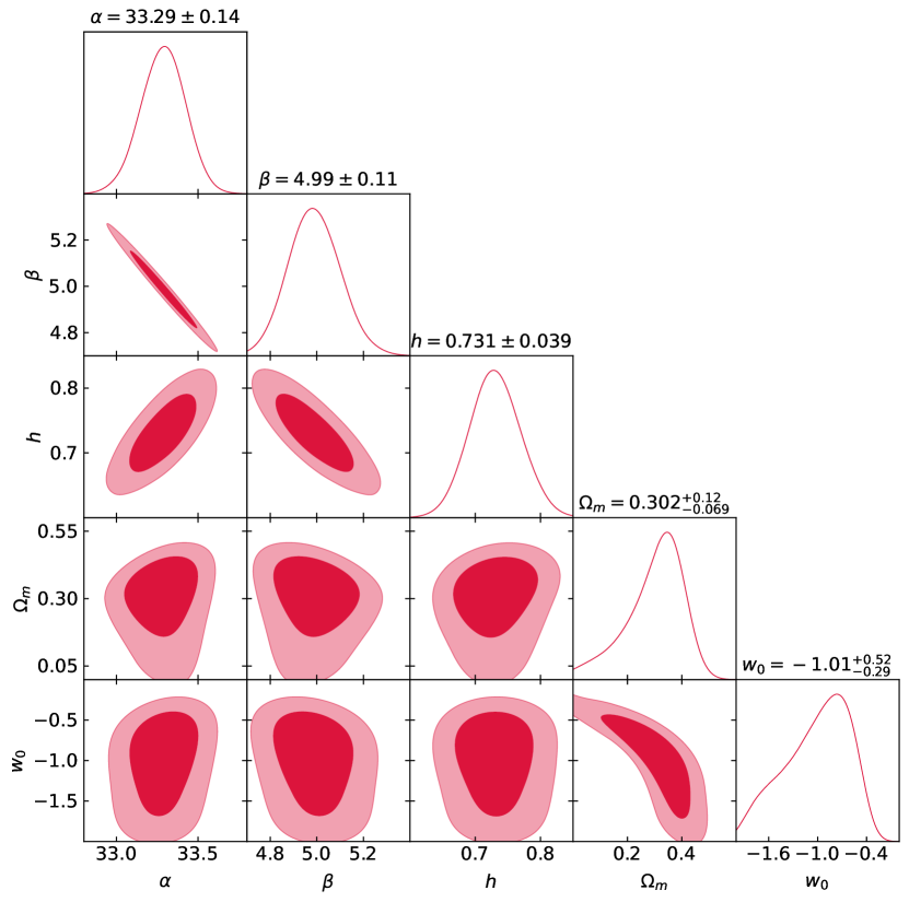
Figure 3: Likelihood contours corresponding to the 1$\sigma$ and 2$\sigma$ confidence levels in the $\{\alpha,\beta,h,\Omega_{m}\,w_{0}\}$ space for the GEHRs and HIIGs sample.

Figure 3 depicts the 1$\sigma$ and 2$\sigma$ likelihood contours derived from a comprehensive global fit applied to our sample of GEHRs and HIIGs. This fit encompasses all free parameters, both nuisance and cosmological, within the framework of a model featuring an evolving DE EoS parameter. The resultant parameter space constraints, as elucidated in this figure and also from Table 1, demonstrate a high degree of consistency with other recent determinations in the field [29, 30]. A comparative analysis of the Figure of Merit ($FoM$) with that reported in [18] reveals a notable improvement of approximately 6.7% in our results.

Discussion and conclusions

The observation that the $\text{L}-\sigma$ relation remains valid in high-redshifts ($z>3$) HIIGs, extending to the epoch of reionization, unveils a remarkable uniformity in H II galaxy properties over vast cosmic timescales. This continuity is not just a testament to the robustness of the $L-\sigma$ relation as a cosmological tool but also illuminates the fundamental processes governing formation and evolution of galaxies in the early Universe.

This result has also profound implications for our understanding of star formation processes in the early Universe. It suggests that the photo-kinematical properties of massive young clusters, which ionise GEHRs and HIIGs, have remained unchanged for most of the age of the Universe. This conclusion challenges models and assumptions about the non-universality of star formation mechanisms [31, 32].

The constraints on cosmological parameters deduced from our dataset, as delineated in Table 1 and Figure 3, specifically our constraints on the space $\{h,\Omega_{m},w_{0}\}=\{0.731\pm 0.039,0.302^{+0.12}_{-0.069},-1.01^{+0.52}_{-0.29}\}$ (stat) from GHIIR and HIIG alone, are closely aligned with the latest results from the Pantheon+ analysis of 1550 SNIa $\{h,\Omega_{m},w_{0}\}=\{0.735\pm 0.011,0.334\pm 0.018,-0.90\pm 0.14\}$ [30]. This concordance underscores the robustness and relevance of our findings in the broader context of contemporary cosmological research.

In our endeavour to refine the determination of cosmological parameters using HIIGs, the incorporation of additional data from the JWST up to and above $z\sim 9$ promises to be invaluable. The unparalleled sensitivity and resolution of JWST, capable of probing the early Universe, offer an unprecedented opportunity to observe HIIGs at higher redshifts. This extended observational reach is pivotal, as it allows for the exploration of the Universe’s expansion dynamics under different cosmological conditions, thereby providing a more comprehensive understanding of the evolution of $\Omega_{m}$, the matter density parameter, and $w_{0}$, the dark energy equation of state parameter.

The potential to observe distant HIIGs with JWST not only complements existing datasets but also enhances the statistical power of our analyses. By extending the redshift range, we can test the consistency of the $\Lambda$CDM model over a broader epoch and scrutinise the possible evolution of dark energy. Moreover, this approach addresses potential biases inherent in current datasets, predominantly stemming from their limited redshift range. The increased sample size, spanning a wider range of cosmic history, is crucial for reducing statistical uncertainties and refining the constraints on $\{h,\Omega_{m},w_{0}\}$.

Further observations from JWST will enable a more detailed examination of the intrinsic properties of HIIGs. This deeper insight is essential for the calibration of the $\text{L}-\sigma$ relation and possible mitigation of systematic uncertainties on the derived parameters. By enhancing our understanding of the physical processes governing HIIGs, we can better interpret their $\text{L}-\sigma$ relation, a fundamental factor in the measurement of cosmological parameters.

Our analysis introduces novel insights into the evolution of the Universe. By leveraging this new data, we significantly enhance the existing narrative of cosmic history. Our results add to the understanding of the early Universe conditions and their role in the formation and evolution of galaxies setting the stage for expanding the exploration of the photo-kinematical properties of massive regions of star formation.

Methods

Data sets

The dataset employed in this study is derived from a comprehensive compilation of data sourced from multiple previously published works:

• The anchor sample of 36 GEHRs was first presented and studied in [26].

• At low $z$ ($0.01\leq z\leq 0.15$), we use 107 HIIGs extensively analysed in [9].

• At intermediate $z$ ($0.6\leq z\leq 4$) we included 24 HIIGs from [33], [34] and [35], our 6 HIIGs observed with VLT-XShooter published in [36], 15 HIIGs observed with Keck-MOSFIRE and presented in [17] and 29 HIIGs observed with VLT-KMOS and presented in [18]. Here we also include 9 new HIIGs first presented in [27].

• At high $z$ ($4\leq z\leq 7.5$) we include 5 new HIIGs observed with JWST-NIRSpec as part of the JWST Advanced Deep Extragalactic Survey (JADES) [37] and first presented in [28].

In Table 2 we present the newly collected data for HIIGs, which extends our previously published data. This dataset integrates the 5 HIIGs observed through JWST-NIRSpec, as described in [28], along with 9 HIIGs from [27]. Recognising the well-documented disparity in the velocity dispersion measurements ($\sigma$) between the [OIII] line and the Balmer lines, a correction of $2.1\ \mathrm{km\ s^{-1}}$ [16] derived from data with both measurements, was applied to the three JWST-NIRSpec HIIGs which do not have $\sigma$ measured from Balmer emission lines. Additionally, we performed extinction corrections on all the H$\beta$ flux measurements, following the extinction law in [38]. The Balmer decrement, derived from H$\alpha$ and H$\beta$ fluxes, was primarily used in the JWST-NIRSpec data and most of the VUDS/VANDELS dataset [27] for extinction correction. In the cases where H$\alpha$ fluxes were unavailable, the mean extinction value from the VUDS/VANDELS data was applied.

Constraints on Cosmological parameters

To rigorously define the cosmological parameters within the scope of this study, we employ a refined methodology, building upon the foundational approaches delineated in our preceding works [16, 17]. A succinct overview of this methodology is presented below to facilitate a comprehensive understanding.

The likelihood function employed for the analysis of GEHRs and HIIGs is expressed as:

$$\mathcal{L}_{H}\propto\exp{\left(-\frac{1}{2}\chi^{2}_{H}\right)}\;,$$ (1)

where the chi-squared ($\chi^{2}_{H}$) term is defined by:

$$\chi^{2}_{H}=\sum_{n}\frac{\left(\mu_{o}(\log f,\log\sigma|\alpha,\beta)-\mu_{\theta}(z|\theta)\right)^{2}}{\epsilon^{2}}\;.$$ (2)

In these expressions, $\mu_{o}$ represents the observed distance modulus, derived from the observables via the $\text{L}-\sigma$ relation, and $\mu_{\theta}$ denotes, for HIIGs the distance modulus derived from a cosmological model with parameters $\theta$ and the measured redshift $z$, while for our calibration sample of GEHRs it represents the distance modulus measured via a primary distance indicator. The parameters $\alpha$ and $\beta$ correspond to the intercept and slope, respectively, of the $\text{L}-\sigma$ relation. Here, $\sigma$ indicates the velocity dispersion, corrected for broadening, and $f$ represents the flux, corrected for extinction.

In Equation 2, the theoretical distance modulus, $\mu_{\theta}$, is a function of a set of cosmological parameters. In the broadest scenario considered in this study, these parameters are denoted as $\theta=\{h,\Omega_{m},w_{0},w_{a}\}$, in addition to the redshift, $z$. The parameters $w_{0}$ and $w_{a}$ are pivotal in defining the DE EoS. The general form of the DE EoS is given by:

$$p_{w}=w(z)\rho_{w}c^{2},$$ (3)

where $p_{w}$ represents the pressure, and $\rho_{w}$ denotes the density of the DE. The function $w(z)$ characterises the evolving DE EoS parameter. Various DE models have been proposed and explored, many of which employ a Taylor expansion around the present epoch. A notable example is the Chevallier-Polarski-Linder (CPL) model [23, 24, 25, 39, 40], which is expressed as:

$$w(z)=w_{0}+w_{a}\frac{z}{1+z}.$$ (4)

The cosmological constant, denoted as $\Lambda$, is just a special case of DE, given for $(w_{0},w_{a})=(-1,0)$, while the so called wCDM models are such that $w_{a}=0$ but $w_{0}$ can take values $\neq-1$.

In the likelihood function, the weights are quantified by $\epsilon^{2}$, which encapsulates various sources of uncertainties. This is formally represented as:

$$\epsilon^{2}=\epsilon^{2}_{\mu_{o},\text{stat}}+\epsilon^{2}_{\mu_{\theta},\text{stat}}+\epsilon^{2}_{\text{sys}},$$ (5)

where $\epsilon_{\mu_{o},\text{stat}}$ denotes the statistical uncertainties of the observed distance modulus, defined by:

$$\epsilon^{2}_{\mu_{o},\text{stat}}=6.25\left(\epsilon_{\log f}^{2}+\beta^{2}\epsilon_{\log\sigma}^{2}+\epsilon_{\beta}^{2}\log\sigma^{2}+\epsilon_{\alpha}^{2}\right).$$ (6)

Here, $\epsilon_{\log f}$, $\epsilon_{\log\sigma}$, $\epsilon_{\alpha}$, and $\epsilon_{\beta}$ represent the uncertainties associated with the logarithm of the flux, the logarithm of the velocity dispersion, and the intercept and slope of the $\text{L}-\sigma$ relation, respectively. Furthermore, $\epsilon_{\mu_{\theta},\text{stat}}$ in Equation 5 refers to the statistical uncertainty associated with the theoretical distance modulus. This uncertainty originates from the redshift uncertainty in the case of HIIGs, and from the primary distance indicator measurement uncertainty for GEHRs. Lastly, $\epsilon_{\text{sys}}$ encompasses the systematic uncertainties.

In the pursuit of a more versatile analysis framework, we have also established an $h$-free likelihood function, as suggested by [41]. This involves a rescaling of the luminosity distance ($d_{L}$) through the introduction of a dimensionless luminosity distance, $D_{L}(z,\theta)$, defined as:

$$D_{L}(z,\theta)=(1+z)\int_{0}^{z}{\frac{dz^{{}^{\prime}}}{E(z^{{}^{\prime}},\theta)}}$$ (7)

In this formulation, $d_{L}$ is expressed as $d_{L}=cD_{L}/H_{0}$. This rescaling technique is employed to ascertain cosmological parameters independently of the Hubble constant, a methodology comprehensively detailed in [17]. Here $E(z,\theta)$ for a flat Universe is given by:

$$E^{2}(z,\theta)=\Omega_{r}(1+z)^{4}+\Omega_{m}(1+z)^{3}+\Omega_{w}(1+z)^{3y}\exp\left(\frac{-3w_{a}z}{1+z}\right)$$ (8)

with $y=(1+w_{0}+w_{a})$ and $\Omega_{r}$ the radiation density parameter such that we can define $\Omega_{w}=1-\Omega_{m}-\Omega_{r}$.

In our analysis, we employ the MultiNest Bayesian inference algorithm [19, 20, 21] to optimise the likelihood function, thereby deriving constraints on various combinations of nuisance and cosmological parameters. Uniform uninformative priors are consistently utilised in all cases [cf. 18].

In order to facilitate a comprehensive comparison of our derived constraints with existing studies, we have adopted the figure of merit ($FoM$) as defined by Wang (2008) [42]. This $FoM$ is quantitatively expressed as:

$$FoM=\frac{1}{\sqrt{\text{det}\ \text{Cov}(\theta_{0},\theta_{1},\theta_{2},\ldots)}}$$ (9)

Here, $\text{Cov}(\theta_{0},\theta_{1},\theta_{2},\ldots)$ represents the covariance matrix corresponding to the parameter set $\{\theta_{i}\}$. This metric provides a robust quantitative basis for evaluating and comparing the precision of different cosmological parameter estimations.

Table 1 presents the derived constraints on various cosmological and nuisance parameters, utilising our comprehensive dataset. This table encompasses combined analyses of both HIIGs and GEHRs samples, as well as scenarios where only the HIIGs sample is employed. In the table, values enclosed in parentheses denote parameters that remained fixed during the analysis.

Data availability

The datasets supporting the conclusions of this article, including the data used for generating the figures, are available from the corresponding author upon reasonable request.

Author contributions statement

RCh, RT and ET led the writing of this paper. ALG-M and DF-A contributed to the writing and to the analysis of the results. RT contributed to the target selection. MLl provided data of HIIG at $z{\sim}3$. FB,MP,SB and RA contributed to the discussion on the physical interpretation of the results.
All authors reviewed the manuscript.

Additional information

Competing interests: The authors declare no competing interests.

Table 1: Marginalised best-fit parameter values and associated $1\sigma$ uncertainties for the HIIGs and GEHRs samples. Values enclosed in parentheses indicate parameters that were held constant during the analysis.

Data Set	$\alpha$	$\beta$	$h$	$\Omega_{m}$	$w_{0}$	$w_{a}$	N
HIIG	—	($5.022\pm 0.058$)	—	$0.282^{+0.037}_{-0.045}$	(-1.0)	(0.0)	195
HIIG	—	($5.022\pm 0.058$)	—	$0.278^{+0.092}_{-0.051}$	$-1.21^{+0.45}_{-0.40}$	(0.0)	195
HIIG	($33.268\pm 0.083$)	($5.022\pm 0.058$)	$0.715\pm 0.018$	$0.267^{+0.038}_{-0.048}$	(-1.0)	(0.0)	195
HIIG	($33.268\pm 0.083$)	($5.022\pm 0.058$)	$0.718\pm 0.020$	$0.278^{+0.091}_{-0.050}$	$-1.22^{+0.46}_{-0.40}$	(0.0)	195
GEHR+HIIG	$33.28\pm 0.11$	$4.997\pm 0.089$	$0.730\pm 0.038$	(0.3)	(-1.0)	(0.0)	231
GEHR+HIIG	$33.28\pm 0.14$	$5.00\pm 0.11$	$0.730\pm 0.040$	$0.335^{+0.044}_{-0.055}$	(-1.0)	(0.0)	231
GEHR+HIIG	$33.29\pm 0.14$	$4.99\pm 0.11$	$0.731\pm 0.039$	$0.302^{+0.12}_{-0.069}$	$-1.01^{+0.52}_{-0.29}$	(0.0)	231
GEHR+HIIG	$33.29\pm 0.14$	$4.99\pm 0.11$	$0.730\pm 0.039$	$0.321^{+0.10}_{-0.063}$	$-0.91^{+0.55}_{-0.33}$	$-0.71^{+0.65}_{-1.2}$	231

Table 2: Data set measurements used in the analysis.

Object	$z$	$\log\sigma$	$\log f(\mathrm{H}\beta)$	$EW(\mathrm{H}\beta)$
		($\mathrm{km\ s^{-1}}$)	($\mathrm{erg\ s^{-1}\ cm^{-2}}$)	($\mathrm{\AA}$)
JWST data
JADES-NS-00016745	$5.56616\pm 0.00011^{a}$	$1.731\pm 0.016^{b}$	$-17.64\pm 0.21^{d}$	$135.35\pm 10.47^{f}$
JADES-NS-10016374	$5.50411\pm 0.00007^{a}$	$1.785\pm 0.014^{b}$	$-18.14\pm 0.20^{d}$	$212.74\pm 12.53^{f}$
JADES-NS-00019606	$5.88979\pm 0.00008^{a}$	$1.622\pm 0.019^{c}$	$-18.11\pm 0.27^{d}$	$242.15\pm 48.25^{f}$
JADES-NS-00022251	$5.79912\pm 0.00007^{a}$	$1.621\pm 0.011^{c}$	$-17.86\pm 0.11^{d}$	$208.52\pm 9.64^{f}$
JADES-NS-00047100	$7.43173\pm 0.00015^{a}$	$1.868\pm 0.024^{c}$	$-17.62\pm 0.39^{e}$
VUDS data
5101421970	$2.4710\pm 0.00025^{g}$	$1.706\pm 0.022^{g}$	$-16.35\pm 0.14^{h}$	$~{}49.72\pm 3.01^{h}$
510996058	$2.4935\pm 0.00025^{g}$	$1.740\pm 0.094^{g}$	$-16.62\pm 0.42^{h}$	$~{}50.55\pm 13.64^{h}$
511001501	$2.2247\pm 0.00022^{g}$	$1.779\pm 0.028^{g}$	$-16.05\pm 0.08^{h}$	$197.56\pm 10.72^{h}$
5101444192	$3.4205\pm 0.00034^{g}$	$1.845\pm 0.017^{g}$	$-16.31\pm 0.16^{h}$	$144.67\pm 25.55^{h}$
VANDELS data
UDS022487	$3.0679\pm 0.00031^{g}$	$1.710\pm 0.031^{g}$	$-16.55\pm 0.15^{h}$	$85.33\pm 8.95^{h}$
CDFS020954	$3.4993\pm 0.00035^{g}$	$1.761\pm 0.085^{g}$	$-16.42\pm 0.14^{h}$	$152.87\pm 8.2^{h}$
CDFS022799	$2.5457\pm 0.00025^{g}$	$1.787\pm 0.017^{g}$	$-16.31\pm 0.07^{h}$	$~{}~{}80.3\pm 3.83^{h}$
UDS020394	$3.3076\pm 0.00033^{g}$	$1.842\pm 0.014^{g}$	$-16.72\pm 0.15^{h}$	$125.37\pm 19.01^{h}$
CDFS018182	$2.3174\pm 0.00023^{g}$	$1.850\pm 0.016^{g}$	$-16.37\pm 0.08^{h}$	$50.43\pm 2.57^{h}$

References

- \bibcommenthead
- [1] Riess, A. G. et al. Observational Evidence from Supernovae for an Accelerating Universe and a Cosmological Constant. AJ 116, 1009–1038 (1998).
- [2] Perlmutter, S. et al. Measurements of Omega and Lambda from 42 High-Redshift Supernovae. ApJ 517, 565–586 (1999).
- [3] Peebles, P. J. E. & Ratra, B. Cosmology with a Time-Variable Cosmological “Constant”. ApJ 325, L17 (1988).
- [4] Wetterich, C. Cosmology and the fate of dilatation symmetry. Nuclear Physics B 302, 668–696 (1988).
- [5] Searle, L. & Sargent, W. L. W. Inferences from the Composition of Two Dwarf Blue Galaxies. ApJ 173, 25–+ (1972).
- [6] Bergeron, J. Characteristics of the blue stars in the dwarf galaxies I ZW 18 and II ZW 40. ApJ 211, 62–67 (1977).
- [7] Terlevich, R. & Melnick, J. The dynamics and chemical composition of giant extragalactic H II regions. MNRAS 195, 839–851 (1981).
- [8] Kunth, D. & Östlin, G. The most metal-poor galaxies. A&A Rev. 10, 1–79 (2000).
- [9] Chávez, R. et al. The L- relation for massive bursts of star formation. MNRAS 442, 3565–3597 (2014).
- [10] Dorner, B. et al. A model-based approach to the spatial and spectral calibration of nirspec onboard jwst. A&A 592, A113 (2016). URL https://doi.org/10.1051/0004-6361/201628263.
- [11] Gardner, J. P. et al. The James Webb Space Telescope. Space Sci. Rev. 123, 485–606 (2006).
- [12] Terlevich, R. & Melnick, J. The dynamics and chemical composition of giant extragalactic H II regions. Monthly Notices of the Royal Astronomical Society 195, 839–851 (1981).
- [13] Melnick, J., Terlevich, R. & Moles, M. Giant H II regions as distance indicators. II - Application to H II galaxies and the value of the Hubble constant. Monthly Notices of the Royal Astronomical Society 235, 297–313 (1988).
- [14] Bordalo, V. & Telles, E. The L- Relation of Local H II Galaxies. ApJ 735, 52 (2011).
- [15] Plionis, M. et al. A strategy to measure the dark energy equation of state using the H II galaxy Hubble function and X-ray active galactic nuclei clustering: preliminary results. MNRAS 416, 2981–2996 (2011).
- [16] Chávez, R. et al. Constraining the dark energy equation of state with H II galaxies. MNRAS 462, 2431–2439 (2016).
- [17] González-Morán, A. L. et al. Independent cosmological constraints from high-z H II galaxies. MNRAS 487, 4669–4694 (2019).
- [18] González-Morán, A. L. et al. Independent cosmological constraints from high-z H II galaxies: new results from VLT-KMOS data. MNRAS 505, 1441–1457 (2021).
- [19] Feroz, F. & Hobson, M. P. Multimodal nested sampling: an efficient and robust alternative to Markov Chain Monte Carlo methods for astronomical data analyses. MNRAS 384, 449–463 (2008).
- [20] Feroz, F., Hobson, M. P. & Bridges, M. MULTINEST: an efficient and robust Bayesian inference tool for cosmology and particle physics. MNRAS 398, 1601–1614 (2009).
- [21] Feroz, F., Hobson, M. P., Cameron, E. & Pettitt, A. N. Importance Nested Sampling and the MultiNest Algorithm. ArXiv e-prints (2013).
- [22] Ratra, B. & Peebles, P. J. E. Cosmological consequences of a rolling homogeneous scalar field. Phys. Rev. D 37, 3406–3427 (1988). URL https://link.aps.org/doi/10.1103/PhysRevD.37.3406.
- [23] Chevallier, M. & Polarski, D. Accelerating Universes with Scaling Dark Matter. International Journal of Modern Physics D 10, 213–223 (2001).
- [24] Linder, E. V. Exploring the Expansion History of the Universe. Physical Review Letters 90, 091301–+ (2003).
- [25] Peebles, P. J. & Ratra, B. The cosmological constant and dark energy. Reviews of Modern Physics 75, 559–606 (2003).
- [26] Fernández Arenas, D. et al. An independent determination of the local Hubble constant. MNRAS 474, 1250–1276 (2018).
- [27] Llerena, M. et al. Ionized gas kinematics and chemical abundances of low-mass star-forming galaxies at z 3. A&A 676, A53 (2023).
- [28] de Graaff, A. et al. Ionised gas kinematics and dynamical masses of galaxies from JADES/NIRSpec high-resolution spectroscopy. arXiv e-prints arXiv:2308.09742 (2023).
- [29] Scolnic, D. M. et al. The Complete Light-curve Sample of Spectroscopically Confirmed SNe Ia from Pan-STARRS1 and Cosmological Constraints from the Combined Pantheon Sample. ApJ 859, 101 (2018).
- [30] Brout, D. et al. The Pantheon+ Analysis: Cosmological Constraints. ApJ 938, 110 (2022).
- [31] Bastian, N., Covey, K. R. & Meyer, M. R. A Universal Stellar Initial Mass Function? A Critical Look at Variations. ARA&A 48, 339–389 (2010).
- [32] Ziegler, J. J. et al. Non-universal stellar initial mass functions: large uncertainties in star formation rates at z 2-4 and other astrophysical probes. MNRAS 517, 2471–2484 (2022).
- [33] Erb, D. K. et al. The Stellar, Gas, and Dynamical Masses of Star-forming Galaxies at z ~ 2. ApJ 646, 107–132 (2006).
- [34] Masters, D. et al. Physical Properties of Emission-line Galaxies at z ~ 2 from Near-infrared Spectroscopy with Magellan FIRE. ApJ 785, 153 (2014).
- [35] Maseda, M. V. et al. The Nature of Extreme Emission Line Galaxies at z = 1-2: Kinematics and Metallicities from Near-infrared Spectroscopy. ApJ 791, 17 (2014).
- [36] Terlevich, R. et al. On the road to precision cosmology with high-redshift H II galaxies. MNRAS 451, 3001–3010 (2015).
- [37] Bunker, A. J. et al. JADES NIRSpec Initial Data Release for the Hubble Ultra Deep Field: Redshifts and Line Fluxes of Distant Galaxies from the Deepest JWST Cycle 1 NIRSpec Multi-Object Spectroscopy. arXiv e-prints arXiv:2306.02467 (2023).
- [38] Gordon, K. D., Clayton, G. C., Misselt, K. A., Landolt, A. U. & Wolff, M. J. A Quantitative Comparison of the Small Magellanic Cloud, Large Magellanic Cloud, and Milky Way Ultraviolet to Near-Infrared Extinction Curves. ApJ 594, 279–293 (2003).
- [39] Dicus, D. A. & Repko, W. W. Constraints on the dark energy equation of state from recent supernova data. Phys. Rev. D 70, 083527 (2004).
- [40] Wang, Y. & Mukherjee, P. Robust Dark Energy Constraints from Supernovae, Galaxy Clustering, and 3 yr Wilkinson Microwave Anisotropy Probe Observations. ApJ 650, 1–6 (2006).
- [41] Nesseris, S. & Perivolaropoulos, L. Comparison of the legacy and gold type Ia supernovae dataset constraints on dark energy models. Phys. Rev. D 72, 123519 (2005).
- [42] Wang, Y. Figure of merit for dark energy constraints from current observational data. Phys. Rev. D 77, 123525 (2008).
- [43] Baker, W. M. et al. Inside-out growth in the early Universe: a core in a vigorously star-forming disc. arXiv e-prints arXiv:2306.02472 (2023).
Acknowledgements
RCh and DF-A acknowledge support from the CONAHCYT research grant CF2022-320152. MLl acknowledges support from the PRIN 2022 MUR project 2022CB3PJ3 - First Light And Galaxy aSsembly (FLAGS) funded by the European Union – Next Generation EU.