Some aspects of symmetry descent

Abstract

In many cases the symmetry structure of quantum field theories can be neatly encoded into their associated symmetry theory (SymTFT), a topological field theory in one dimension higher. For geometrically engineered QFTs in string theory this SymTFT has been argued to arise from the background geometry, essentially by integration of the topological sector of string theory on the horizon of the geometry transverse to the QFT locus. In this paper we clarify some subtle aspects of this proposal. We take a higher dimensional approach, where the ten dimensional string theory fields to be integrated arise as edge modes of a topological field theory in eleven dimensions. The resulting construction provides a SymTFT generalisation of the descent procedure for anomalies.

1 Introduction

A complete definition of any given Quantum Field Theory requires information both about local dynamics, and about its topological sector: in general, the same set of local degrees of freedom can be coupled to different topological sectors. From a modern point of view, we consider any topological operator in the Quantum Field Theory a symmetry (in a suitably generalised sense), so an equivalent restatement of the previous remark is that theories with the same local dynamics might have different sets of symmetries Gaiotto:2010be ; Aharony:2013hda ; Kapustin:2014gua ; Gaiotto:2014kfa . These choices of symmetries are often related in simple ways. For instance, if we have a $d$-dimensional theory $\mathcal{T}_{d}$ with a finite symmetry group $G$, we can gauge an anomaly-free subgroup $H$ of $G$ and obtain a new theory $\mathcal{T}_{d}/H$, with the same local dynamics but different symmetries. In general $G$ itself need not be anomaly-free, which can lead to some of the symmetry generators in $\mathcal{T}_{d}/H$ to be non-invertible, meaning that for a given operator $\mathcal{O}$ there is no operator $\mathcal{O}^{-1}$ in the theory such that $\mathcal{O}\mathcal{O}^{-1}$ is the identity operator.

This is far from an exotic possibility: the existence of such operators in two dimensions has been understood for many years Frohlich:2009gb ; Carqueville:2012dk ; Brunner:2013xna ; Bhardwaj:2017xup ; Gaiotto:2019xmp , and more recently it has been argued, starting with Gaiotto:2019xmp ; Heidenreich:2021xpr ; Choi:2021kmx ; Kaidi:2021xfk , that the same is true in higher dimensions. We refer the reader to Cordova:2022ruw ; McGreevy:2022oyu ; Freed:2022iao ; Schafer-Nameki:2023jdn ; Brennan:2023mmt ; Bhardwaj:2023kri ; Shao:2023gho for reviews, and pointers to the extensive literature. This process can be continued: $\mathcal{T}_{d}/H$ will have its own set of symmetries, and we can gauge a subset of these, leading to a new theory, and so on. We refer to a choice of representative in this set of related theories as a choice of global form.

The discussion in the previous paragraph is somewhat unsatisfactory, in that it started from a theory $\mathcal{T}_{d}$ with “ordinary” group-like symmetries, and we accessed more interesting symmetry structures by sequences of gaugings. But in general, there is no requirement that a canonical choice for $\mathcal{T}_{d}$ exists, and in fact, it is possible that none of the set of theories related by gauging operations has group-like symmetries only. A better viewpoint is available Ji:2019jhk ; Gaiotto:2020iye ; Apruzzi:2021nmk ; Freed:2022qnc ; Kaidi:2022cpf ; Kaidi:2023maf ; Bhardwaj:2023wzd ; Baume:2023kkf ; Brennan:2024fgj ; Antinucci:2024zjp ; Bonetti:2024cjk ; DelZotto:2024tae ; Bhardwaj:2024qrf ; Cordova:2024vsq ; Nardoni:2024sos ; Argurio:2024oym : instead of considering each $d$-dimensional theory with the same local dynamics as $\mathcal{T}_{d}$, we study a $(d+1)$-dimensional topological field theory $\mathsf{Symm}_{d+1}$ (which we call the symmetry theory, or SymTFT, as in Apruzzi:2021nmk ) which admits a gapless boundary condition with the same local dynamics as $\mathcal{T}_{d}$. We denote this gapless boundary condition (which should be understood as a relative quantum field theory Freed:2012bs ) encoding the local dynamics of $\mathcal{T}_{d}$ as $\Lambda(\mathcal{T}_{d})$. All theories related by gauging of finite symmetries lead to the same $\Lambda(\mathcal{T}_{d})$. This configuration in itself should be thought of as a $(d+1)$-dimensional theory on a space with boundary, but it can be turned into a definition for a $d$-dimensional field theory with the same local dynamics as $\mathcal{T}_{d}$ if $\mathsf{Symm}_{d+1}$ admits a gapped interface $\iota_{d}$ to an anomaly theory $\mathcal{A}_{d+1}$. Pictorially, we have:

We obtain a $d$-dimensional theory with anomaly $\mathcal{A}_{d+1}$ by colliding $\iota_{d}$ with $\Lambda(\mathcal{T}_{d})$. Different choices of global form for $\mathcal{T}_{d}$ correspond to different choices of the pair $(\mathcal{A}_{d+1},\iota_{d})$: some of the topological operators in $\mathsf{Symm}_{d+1}$ will become trivial when we collapse $\iota_{d}$ and $\Lambda(\mathcal{T}_{d})$, but some will survive as symmetries of the resulting field theory. In this way, we have reformulated the problem of understanding all theories related to $\mathcal{T}_{d}$ and their symmetries into two parts: first determining $\mathsf{Symm}_{d+1}$ given $\mathcal{T}$ (or $\Lambda(\mathcal{T}_{d})$) and then classifying the pairs $(\mathcal{A}_{d+1},\iota_{d})$ that $\mathsf{Symm}_{d+1}$ can attach to.

Our focus in this paper will be on supersymmetric quantum field theories obtained by placing string theory or M-theory at isolated conical singularities of the form $C(L)$, with $L$ the base of the cone. This class of configurations leads to superconformal field theories living at the singular base of the cone. Generically these superconformal theories do not admit any weakly coupled description, so we have very poor knowledge of $\Lambda(\mathcal{T}_{d})$. Nevertheless, it was argued in Apruzzi:2021nmk (see also Bah:2019rgq ; Bah:2020jas for related earlier works) that $\mathsf{Symm}_{d+1}$ can be obtained (in the M-theory case) by performing a reduction of the topological terms in the M-theory action on $L$, which reduces the computation to a somewhat technical but fully solvable problem in algebraic topology.

Our main goal in this paper is to clarify one issue in the analysis of Apruzzi:2021nmk that remained somewhat puzzling: while the terms in $\mathsf{Symm}_{d+1}$ related to anomalies were computed via a straightforward integration on $L$, there was also a $BF$ sector, schematically of the form

$$\begin{split}S_{BF}(B,A)=2\pi iN\int B\wedge dA\,,\end{split}$$ (1)

that had to be computed used entirely different (and somewhat indirect) methods. Our goal in this note is to bring the two viewpoints closer together by explaining how this $BF$ theory can be derived by integration on $L$ of an auxiliary theory in one dimension higher.

Let us briefly review how Apruzzi:2021nmk argues for the existence of a $BF$ sector in $\mathsf{Symm}_{d+1}$. The basic setup is string theory or M-theory on a Calabi-Yau cone $C(L)$ with Sasaki-Einstein base $L$ times a manifold $\mathcal{M}^{d}$:

In M-theory $\dim(L)=10-d$ and in type II string theory $\dim(L)=9-d$. We will assume that the singular locus of $C(L)$ consists of an isolated singularity at the tip of the cone, and that $\mathcal{M}^{d}$ is spin and torsion-free. There are light degrees of freedom living at the singular locus of $C(L)$, which in the examples studied in Apruzzi:2021nmk lead to a $d$-dimensional SCFT living on $\mathcal{M}^{d}$. As argued in GarciaEtxebarria:2019caf , the information given so far defines only the local data of the SCFT (namely, the relative theory we have denoted by $\Lambda(\mathcal{T}_{d})$ in the introduction) and the rest of the data necessary for fully defining a SCFT $\mathcal{T}_{d}$ are instead encoded in a choice of boundary condition at infinity for the supergravity fields on $\mathcal{M}^{d}\times C(L)$.

One of the main results of Apruzzi:2021nmk is to reconcile this picture, which is very natural from a string theory point of view, with the SymTFT viewpoint described in the introduction. The basic idea is that $\mathsf{Symm}_{d+1}$ arises from reducing the topological sector of string theory over the base of the cone $C(L)$:

In this proposal, we identify the tip of the cone with the gapless boundary $\Lambda(\mathcal{T}_{d})$, and the boundary conditions at infinity with the pair $(\mathcal{A}_{d+1},\iota_{d})$.

It was shown in Apruzzi:2021nmk that a subsector of $\mathsf{Symm}_{d+1}$ (leading to $\mathcal{A}_{d+1}$ for suitable choices of boundary conditions) arises quite naturally from integrating the Chern-Simons term in the M-theory action over $L$.

The $BF$ sector in $\mathsf{Symm}_{d+1}$ is more subtle. For concreteness we consider, as in Apruzzi:2021nmk , the case of $d=5$ SCFTs arising from putting M-theory on singular Calabi-Yau threefolds. As studied in Morrison:2020ool ; Albertini:2020mdx , the local dynamics for these SCFTs can be completed to theories with either 1-form or 2-form symmetries, and the boundary conditions for the $BF$ subsector of $\mathsf{Symm}_{6}$ determine which kind of symmetries we have. The 1-form symmetries have generators coming from $G_{4}$ fluxes and the 2-form symmetries from the $G_{7}$ fluxes (under the kind of identification reviewed in footnote 6, and explained in more detail in GarciaEtxebarria:2019caf . These flux generators do not commute with one another Moore:2004jv ; Freed:2006ya ; Freed:2006yc , and as a result, when choosing boundary conditions we need to choose to which of $G_{4}$ or $G_{7}$ we give Dirichlet boundary conditions, we cannot give Dirichlet boundary conditions to both. In terms of the field theory we have that we cannot realise both the 1-form and 2-form symmetry at the same time. This hints at the fact that if the $BF$ action was to be obtained from a reduction of a supergravity action, it should be one that contains both the $G_{4}$ and $G_{7}$ fluxes. Ignoring some (crucial) complications from the presence of the Chern-Simons term, the closest object is the kinetic term $\int G_{4}\wedge*G_{4}$, if one observes that $G_{4}$ and $G_{7}$ fluxes are dual to one another in M-theory. This expectation is borne out by the analysis in Apruzzi:2021nmk , which constructs the algebra of topological operators in the $BF$ theory from the reduction on $L$ of the algebra of topological operators in the M-theory background.

The discussion above explains why it is subtle to obtain the expected $BF$ theory from a dimensional reduction: to reproduce the non-commutativity we would need an action that simultaneously describes electric ($G_{4}=dC_{3}$) and magnetic ($G_{7}=dC_{6}$) fluxes. This is closely related, by viewing the pair $(C_{3},C_{6})$ as a two-component field, to the famously difficult problem of writing an action for a self-dual field.

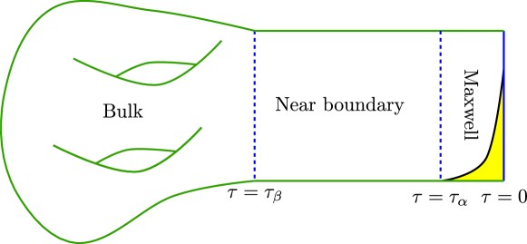
There are multiple ways of approaching the problem of constructing actions, or directly the partition function, for a self-dual field Witten:1996hc ; Witten:1998wy ; Witten:1999vg ; Moore:1999gb ; Freed:2000ta ; Gukov:2004id ; Belov:2004ht ; Belov:2006jd ; Belov:2006xj . In this paper, we approach this problem using a strategy initiated by Witten Witten:1996hc , in which we define the partition function of a self-dual field on $X$ in terms of Chern-Simon theory on $Y$, with $\partial Y=X$. Suitable choices of boundary conditions for the Chern-Simons field (which we discuss in detail below, following Belov:2004ht ; Hsieh:2020jpj ) lead to the emergence of the self-dual degrees of freedom on $X$. From this point of view, our task decomposes into two (simpler) tasks: first we need to reduce the Chern-Simons action on our internal manifold $L$, and then we need to understand how the effective theory arising from reduction on $L$ behaves on a manifold with boundary. This is summarised in figure 1.

Figure 1: We want to understand the emergence of the $BF$ theory on $X$ from compactification of self-dual dynamics on $L$. (Dashed arrow on the left hand side of the diagram.) We do this by promoting the theory on $X\times L$ to a Chern-Simons theory on $Y\times L$, where $\partial Y=X$, integrating this Chern-Simons theory on $L$, and restricting back to $X$.

The central result of our analysis is stated in a precise way in eq. (70) below. Intuitively, what that equation is saying is that there is a form of inflow for the SymTFT:

$$\begin{split}\Delta\int_{L}\mathcal{L}_{BF}=\delta\mathcal{L}_{\mathsf{Symm}}\end{split}$$ (2)

where $\mathcal{L}_{BF}$ and $\mathcal{L}_{\mathsf{Symm}}$ are suitable notions of “Lagrangian densities” for the $BF$ and SymTFT, $\Delta$ denotes gauge transformations, and $\delta$ denotes the exterior derivative. The formalism of Hopkins and Singer Hopkins:2002rd is very useful in making the notion of gauge transformations of Lagrangian densities precise in topologically non-trivial configurations, we review the basics in section 2. A key advantage of this formalism is that it allows us to keep control of topological aspects of the problem in a way that is local. (In physics terms, we will be producing Lagrangian densities, and not just actions.) This allows us to make our formalism actually useful in practice: otherwise, since we are viewing the SymTFT as arising from boundary modes, it would be difficult to place it on spaces with boundary!

We expect that a modification of our approach (replacing ordinary differential cohomology with twisted differential $K$-theory) will allow us to recover not only the $BF$ sector but also the anomaly theory, at least in cases where the mathematical formalism is understood well enough. We provide evidence for this expectation in section 6.

A note on related recent literature: The papers vanBeest:2022fss ; Apruzzi:2022rei ; Lawrie:2023tdz ; Apruzzi:2023uma ; Yu:2023nyn ; Basile:2023zng appeared during the (fairly long) preparation of the results we present here. They include a discussion of ideas related to those in this paper for the derivation of the $BF$ action, among many other interesting results, and in particular they also start from a theory in eleven dimensions (in the string theory case) and propose that the SymTFT can be understood from dimensional reduction of the eleven dimensional theory. Nevertheless, we believe that the analysis in this paper is still useful, as it clarifies many of the subtleties, both technical and conceptual, which we encountered in making this picture precise (for example in giving a precise meaning to equations like (2)) and which were not addressed in the works just mentioned. We will explain in detail which boundary conditions one needs to take in the eleven dimensional theory for the picture to work, how the edge modes — or in other words, the fields in the SymTFT — relate to the dynamical fields in eleven dimensional theory, and explain various subtle aspects of the mathematics involved in the case of topologically non-trivial geometries.

2 Differential cohomology

Our starting point is abelian Chern-Simons theory at level $k$ in $4n+3$-dimensions. The action $S$ for this theory can be written as $S=2\pi i\,\mathsf{CS}_{k}[A]$, with (heuristically)

$$\begin{split}\mathsf{CS}_{k}[A]=\frac{k}{2}\int A\wedge dA\,,\end{split}$$ (3)

where $A$ is a $2n+1$ form. The most familiar case is $n=0$, where the self-dual field on the boundary is a self-dual boson. Eq. (3) is heuristic for three reasons. First, we are using differential form notation for the field $A$, but in the cases of interest to us $A$ cannot be globally defined as a differential form, but it is rather a connection on a topologically non-trivial bundle. The second aspect of (3) that needs clarification is that, in fact, we will be interested mostly in the case of $A$ being a flat connection on a topologically non-trivial bundle. (Our discussion is about IR effects, and non-flat modes in the same topological sector encode massive excitations, which we want to integrate out.) So, naively, $dA=0$. These two complications can be dealt with by switching to the language of differential cohomology. Below we will give a very brief review of the main aspects of this formalism as they apply to our case. The last subtlety in the interpretation of (3) concerns the quantisation of $k$. In general, this Chern-Simons theory makes sense for arbitrary $k\in\mathbb{Z}$, but for odd values of $k$ there is an implicit dependence on the Wu structure of the manifold. In the (oriented) $n=0$ case the Wu structure reduces to the spin structure, and we have the familiar statement that Chern-Simons theory at odd values of $k$ (or half-integral values, depending on conventions) depends on the spin structure. We will address this final subtlety below, after introducing some formalism we need for addressing the first two points.

Since we will need to consider a refinement of connection $A$ itself, and not just the Chern-Simons action itself, we will adopt the formalism of Hopkins–Singer Hopkins:2002rd . Our goal here is simply to set notation and review the basic operational rules. We encourage the reader to read Freed:2000ta ; Hopkins:2002rd ; Hsieh:2020jpj for in-depth discussions.

Consider the cochain complex $\{\breve{C}(n)^{\bullet}(\mathcal{M}),d\}$ with

$$\breve{C}(n)^{p}(\mathcal{M})=\begin{cases}C^{p}(\mathcal{M};\mathbb{Z})\times C^{p-1}(\mathcal{M};\mathbb{R})\times\Omega^{p}(\mathcal{M};\mathbb{R})&\text{for}\quad p\geq n\\ C^{p}(\mathcal{M};\mathbb{Z})\times C^{p-1}(\mathcal{M};\mathbb{R})&\text{for}\quad p<n\end{cases}$$ (4)

and differential

$$\begin{split}d(c,h,\omega)=&\,(\delta c,\omega-c-\delta h,d\omega)\quad\text{for}\quad(c,h,\omega)\in\breve{C}(n)^{p}(\mathcal{M})\\ d(c,h)=&\begin{cases}(\delta c,-c-\delta h,0)&\text{for}\quad(c,h)\in\breve{C}(p)^{p-1}(\mathcal{M})\\ (\delta c,-c-\delta h)&\text{otherwise.}\end{cases}\end{split}$$ (5)

We can alternatively think of elements of $\breve{C}(n)^{p}(\mathcal{M})$ for $p<n$ as triples $(c,h,\omega)$ with $\omega=0$. We call elements of $\breve{C}(n)^{p}(\mathcal{M})$ differential cochains, and define differential cocycles as the closed differential cochains:

$$\breve{Z}(n)^{p}(\mathcal{M})\coloneqq\{\breve{x}\in\breve{C}(n)^{p}(\mathcal{M})\mid d\breve{x}=0\}\,.$$ (6)

For notational convenience, we introduce maps $I$, $\mathsf{h}$ and $R$ such that for the differential cochain $\breve{a}=(c,h,\omega)\in\breve{C}(n)^{p}(\mathcal{M})$

$$\begin{split}\big{(}I(\breve{a}),\mathsf{h}(\breve{a}),R(\breve{a})\big{)}=(c,h,\omega)\,,\end{split}$$ (7)

and define $\breve{C}^{p}(\mathcal{M})\coloneqq\breve{C}(p)^{p}(\mathcal{M})$, $\breve{Z}^{p}(\mathcal{M})\coloneqq\breve{Z}(p)^{p}(\mathcal{M})$.

Finally, we note for future reference that the condition $d\breve{a}=0$ for a cocycle $\breve{a}\in\breve{Z}(n)^{p}(\mathcal{M})$ implies that its components satisfy $\delta\mathsf{h}(\breve{a})=R(\breve{a})-I(\breve{a})$.

The differential cohomology group $\breve{H}(n)^{p}(\mathcal{M})$ is then obtained in the familiar way:

$$\breve{H}(n)^{p}(\mathcal{M})\coloneqq\breve{Z}(n)^{p}(\mathcal{M})/d\breve{C}(n)^{p-1}(\mathcal{M})\,.$$ (8)

The special case $\breve{H}(n)^{n}(\mathcal{M})$ coincides with the Cheeger-Simons differential cohomology group $\breve{H}^{n}(\mathcal{M})$ 10.1007/BFb0075216 . In particular, the Cheeger-Simons differential character $\chi([\breve{x}])\in\mathbb{R}/\mathbb{Z}$ is given by

$$\begin{split}\chi([\breve{x}])=\mathsf{h}(\breve{x})\mod 1\,.\end{split}$$ (9)

Here (and below) we denote elements of $\breve{H}^{n}(\mathcal{M})$ by $[\breve{x}]$, where $\breve{x}\in\breve{Z}(n)^{n}(\mathcal{M})$ is some representative of the differential cohomology class, defined up to an exact cocycle.

The next ingredient we need is a notion of a product between differential cochains, generalising the cup product in differential cohomology. Given two differential cochains $\breve{a}_{1}=(c_{1},h_{1},\omega_{1})$ and $\breve{a}_{2}=(c_{2},h_{2},\omega_{2})$ their product $\breve{a}_{1}\cdot\breve{a}_{2}$ is a new cochain with components

$$(c_{1}\cup c_{2},(-1)^{|c_{1}|}c_{1}\cup h_{2}+h_{1}\cup\omega_{2}+B(\omega_{1},\omega_{2}),\omega_{1}\wedge\omega_{2})\,.$$ (10)

Here $B$ is any natural homotopy between $\wedge$ and $\cup$

$$\delta(B(\omega_{1},\omega_{2}))+B(d\omega_{1},\omega_{2})+(-1)^{|\omega_{1}|}B(\omega_{1},d\omega_{2})=\omega_{1}\wedge\omega_{2}-\omega_{1}\cup\omega_{2}\,.$$ (11)

where we are promoting differential forms to cochains as needed. Note that whenever $\omega_{1}=0$ or $\omega_{2}=0$ we can choose $B(\omega_{1},\omega_{2})=0$ (since the right-hand side of (11) vanishes and this choice of homotopy is certainly natural; or alternatively using the explicit expression given in 10.1007/BFb0075216 ). A straightforward computation shows that for $\breve{a}\in\breve{C}(p)^{q}(\mathcal{M})$, $\breve{b}\in\breve{C}(r)^{s}(\mathcal{M})$ we have

$$\begin{split}d(\breve{a}\cdot\breve{b})=(d\breve{a})\cdot\breve{b}+(-1)^{q}\breve{a}\cdot d(\breve{b})\,,\end{split}$$ (12)

In particular this implies that the product defined above induces a product in differential cohomology classes, which is precisely the product defined by Cheeger and Simons 10.1007/BFb0075216 . We note that, for $\breve{a}$ and $\breve{b}$ cocycles, we have that $\breve{a}\cdot\breve{b}$ and $(-1)^{\deg(\breve{a})\deg(\breve{b})}\breve{b}\cdot\breve{a}$ are equivalent up to gauge transformations.

Given a fibre bundle with closed oriented fibres it is possible to define a notion of integration along the fibre for differential cochains Hopkins:2002rd . In this note, we are only interested in the case of trivial fibrations, namely spaces of the form $\mathcal{M}=B\times F$, where $F$ is a $n$-dimensional, closed and oriented. In this case, we define the integration map

$$\begin{split}\int_{F}\colon\breve{C}(p)^{p}(B\times F)\to C(p-n)^{p-n}(B)\end{split}$$ (13)

given by Green-FM

$$\int_{F}(c,h,\omega)\coloneqq\left(c/F,h/F,\omega/F\right)$$ (14)

where on the slant products spanier1989algebraic on the right hand side we have abused notation (as we will keep doing in this paper), and denoted by $F\in Z_{n}(F)$ the fundamental class of $F$. Given a cochain $c\in C^{n}(B\times F)$ and a chain $v\in C_{p}(F)$ the (bilinear) slant product $c/v\in C^{n-p}(B)$ satisfies $(c/v)(u)=c(u\times v)$ for all $u\in C_{n-p}(B)$. A property of the slant product that we will need later is

$$\begin{split}\delta(c/v)=(\delta c)/v+(-1)^{n-p}c/(\delta v)\,,\end{split}$$ (15)

so the slant product on (co)chains descends to (co)homology. Additionally, viewing $\omega$ as a differential form, $\omega/F$ coincides with the usual notion of integration along $F$. Motivated by this, we will sometimes abuse notation and write $x/F$ as $\int_{F}x$, even when $x$ is a cochain.

So far we have assumed that the fibre is closed. In case the fibre has a boundary the discussion above still goes through, with some modifications described in detail in Hopkins:2002rd . A particularly important result, in this case, is the following version of Stokes’ theorem for $\breve{x}\in\breve{C}(p)^{q}(\mathcal{M})$:

$$d\int_{F}\breve{x}=\int_{F}d\breve{x}+(-1)^{|\breve{x}|-\dim(F)}\int_{\partial F}\breve{x}\,,$$ (16)

which follows from a short computation using (15). If $F$ is closed then this version of Stokes’ theorem implies that integration descends to differential cohomology

$$\begin{split}\int_{F}\colon\breve{H}(p)^{p}(B\times F)\to\breve{H}(p-n)^{p-n}(B)\end{split}$$ (17)

in the obvious way.

Before we proceed any further, let us briefly discuss a few simple examples that illuminate these techniques, and which play an important role below. In all cases we take the base $B$ to be a point, which we denote by “$\mathrm{pt}$”, so our total manifold is $\mathcal{M}\coloneqq\mathrm{pt}\times F\cong F$.

Example 1: $U(1)$ theory in two dimensions

Consider first the case of an ordinary $U(1)$ gauge 1-form connection on a two dimensional manifold $M$. We take the action to be $2\pi i\int_{M}F$ (up to a small refinement we clarify momentarily). This theory is trivial whenever $M$ is closed, but it can be useful when studying Wilson lines on $\partial M$, for instance. We will find it useful to reformulate the action of this theory in the language of differential cohomology as

$$\begin{split}S_{2d}[\breve{a}]=2\pi i\,\mathsf{h}\left(d\int_{M}\breve{a}\right)\,,\end{split}$$ (18)

with $\breve{a}\in\breve{Z}^{2}(M)$. Equivalently, since the action appears in the form $e^{-S_{2d}[\breve{a}]}$ in the path integral, we can write, using (9):

$$\begin{split}\frac{1}{2\pi i}S_{2d}[\breve{a}]=\chi\left(\left[d\int_{M}\breve{a}\right]\right)\mod 1\,.\end{split}$$ (19)

Note that generically $R(\int_{M}\breve{a})=\int_{M}R(\breve{a})\neq 0$, so despite the notation $d\int_{M}\breve{a}$ is not pure gauge, or equivalently $\left[d\int_{M}\breve{a}\right]\in\breve{H}(1)^{1}(\mathrm{pt})$ does not necessarily vanish, and therefore the holonomy (19) is not necessarily trivial.

To see that this gives the action we are after, compute

$$\begin{split}d\int_{M}\breve{a}=d\,(I(\breve{a})/M,0,R(\breve{a})/M)=(0,(R(\breve{a})-I(\breve{a}))/M,0)\end{split}$$ (20)

where on the first equality we have used that $h(\breve{a})/M=0$ for degree reasons, and similarly $\delta I(\breve{a})/M=\delta R(\breve{a})/M=0$ on the second one. Since $I(\breve{a})$ is an integral cochain we find

$$\begin{split}\frac{1}{2\pi i}S_{2d}[\breve{a}]=\mathsf{h}\left(d\int_{M}\breve{a}\right)=(R(\breve{a})-I(\breve{a}))/M=\int_{M}F\mod 1\end{split}$$ (21)

as desired, where $F\coloneqq R(\breve{a})$.

To see why (18) is useful, take $M$ to have non-vanishing boundary $\partial M$. By applying (16) we immediately get

$$\begin{split}S_{2d}[\breve{a}]=2\pi i\,\mathsf{h}\left(\int_{\partial M}\breve{a}\right)\,.\end{split}$$ (22)

So we end up with the holonomy on the boundary, as expected. Note that we have not yet quotiented by gauge transformations, so this holonomy lives in $\mathbb{R}$. We can also obtain the same result starting from (20) and using the fact that $\breve{a}$ is a cocycle (so $d\breve{a}=0$), which then implies $R(\breve{a})-I(\breve{a})=\delta\mathsf{h}(\breve{a})$, so (20) gives $S_{2d}[\breve{a}]=2\pi i\,\delta\mathsf{h}(\breve{a})/M$. Using (15) and the fact that $\mathsf{h}(\breve{a})/M=0$ for degree reasons, we get $S_{2d}[\breve{a}]=2\pi i\,\mathsf{h}(\breve{a})/\partial M$, which agrees with (22).

Consider now gauge transformations, which act on $\breve{a}$ as $\breve{a}\to\breve{a}+d\breve{\lambda}$, with $\breve{\lambda}\in\breve{C}(2)^{1}(M)$. Parameterising $\breve{\lambda}=(c,f,0)$, we have $d\breve{\lambda}=(\delta c,-c-\delta f,0)$, with $f\in C^{0}(M;\mathbb{R})$ and $c\in C^{1}(M;\mathbb{Z})$. This gauge transformation acts on (20) by

$$\begin{split}d\int_{M}\breve{a}\to d\int_{M}\breve{a}+d\int_{M}d\breve{\lambda}=d\int_{M}\breve{a}-\int_{\partial M}d\breve{\lambda}&=(0,(\mathsf{h}(\breve{a})+\delta f+c)/\partial M,0)\\ &=(0,(\mathsf{h}(\breve{a})+c)/\partial M,0)\,.\end{split}$$ (23)

We recognise the term $\delta f$ as the one generating small gauge transformations. These do not affect the value of this integral (since $\delta f/\partial M=\delta(f/\partial M)=0$ for degree reasons). On the other hand, $c$ is the part that generates large gauge transformations on the boundary, and such transformations do change the value of the action. Since $c$ is an integral cochain, the change is by integer multiples of $2\pi i$, so it does not affect the physics.

Example 2: $U(1)\times U(1)$ theory in even dimensions

As a slightly more elaborate version of this example, consider the case where $B$ is still a point, which we denote by “$\mathrm{pt}$”, $\dim(F)=2n$, and we want to define a theory with action

$$\begin{split}S_{k}\coloneqq 2\pi i\,k\int_{F}F_{1}\wedge F_{2}\,,\end{split}$$ (24)

where $F_{1}$ and $F_{2}$ are field strengths of degree $n$ for abelian higher form fields. An important application of such an action is in defining a discrete gauge $\mathbb{Z}_{k}$ theory Banks:2010zn on $\partial F$ in terms of a bulk theory on $F$. (See also example 3 below.) As in the previous example, we reformulate this action in differential cohomology as

$$\begin{split}S_{k}=2\pi i\,k\,\mathsf{h}\left(d\int_{F}\breve{a}_{1}\cdot\breve{a}_{2}\right)\,,\end{split}$$ (25)

where $\breve{a}_{1},\breve{a}_{2}\in\breve{Z}^{n}(F)$. The integral of $\mathsf{h}(\breve{a}_{1}\cdot\breve{a}_{2})\in C^{2n-1}(F;\mathbb{R})$ over $F$ vanishes for dimensional reasons and therefore

$$\int_{F}\breve{a}_{1}\cdot\breve{a}_{2}=(I(\breve{a}_{1}\cdot\breve{a}_{2})/F,0,R(\breve{a}_{2}\cdot\breve{a}_{2})/F)\in\breve{C}(0)^{0}(\mathrm{pt})\cong\mathbb{Z}\times\mathbb{R}\,.$$ (26)

Assume first that $\partial F=0$. Then by Stokes’ formula (16) the result of integration is actually closed under $d$, which implies the familiar relation $I(\breve{a}_{1}\cdot\breve{a}_{2})/F=R(\breve{a}_{1}\cdot\breve{a}_{2})/F$.

More generally, if $F$ has a boundary, (16) gives (similarly to the previous example)

$$\begin{split}d\int_{F}\breve{a}_{1}\cdot\breve{a}_{2}&=d(I(\breve{a}_{1}\cdot\breve{a}_{2})/F,0,R(\breve{a}_{2}\cdot\breve{a}_{2})/F)\\ &=(0,(R(\breve{a}_{1}\cdot\breve{a}_{2})-I(\breve{a}_{1}\cdot\breve{a}_{2}))/F,0)\\ &=(0,\mathsf{h}(\breve{a}_{1}\cdot\breve{a}_{2})/\partial F,0)\,.\end{split}$$ (27)

Coming back to (27), we can rewrite it in more familiar notation:

$$\begin{split}\int_{F}R(\breve{a}_{1})\wedge R(\breve{a}_{2})-\int_{F}I(\breve{A}_{1})\cup I(\breve{a}_{2})=\int_{\partial F}\mathsf{h}(\breve{a}_{1}\cdot\breve{a}_{2})\,.\end{split}$$ (28)

Assuming that $I(\breve{a}_{1})$ is topologically trivial, then there is a globally defined connection $A_{1}\in\Omega^{1}(F)$, and the equation can be written as

$$\begin{split}\int_{F}F_{1}\wedge F_{2}-\int_{F}I(\breve{a}_{1})\cup I(\breve{a}_{2})=\int_{\partial F}A_{1}\wedge F_{2}\end{split}$$ (29)

where we have denoted the field strength $R(\breve{a}_{i})$ by $F_{i}$. Gauge transformations shift the right hand side and left hand sides by (equal) integers, so this equation is often written as

$$\begin{split}\int_{F}F_{1}\wedge F_{2}=\int_{\partial F}A_{1}\wedge F_{2}\mod 1\,.\end{split}$$ (30)

In our derivation below the more abstract version (28) of this equation will play a key role.

It is an illuminating (and important for our later purposes) exercise to check the variation of the integral (26) under gauge transformations of $\breve{a}_{i}$. The latter are given by the ambiguity of $\breve{a}_{i}$ by an exact cocycle $d\breve{b}_{i}\in\breve{Z}^{n}(F)$ with $\breve{b}_{i}\in\breve{C}(n)^{n-1}(F)$. Under these gauge transformations $\breve{a}_{i}\to\breve{a}_{i}+d\breve{b}_{i}$ and (using (12))

$$\begin{split}\breve{a}_{1}\cdot\breve{a}_{2}\to(\breve{a}_{1}+d\breve{b}_{1})\cdot(\breve{a}_{2}+d\breve{b}_{2})=\breve{a}_{1}\cdot\breve{a}_{2}+d\breve{\lambda}\,,\end{split}$$ (31)

with $\breve{\lambda}\coloneqq(-1)^{n}\breve{a}_{1}\cdot\breve{b}_{2}+\breve{b}_{1}\cdot\breve{a}_{2}+(-1)^{n}\breve{d}b_{1}\cdot\breve{b}_{2}$. (There is some ambiguity in the choice of $\breve{\lambda}$, here we pick a representative that simplifies some of the formulas later on.) Note that $R(\breve{\lambda})=0$, since $R(\breve{b}_{i})=0$. Thus, if $\partial F\neq 0$, then by (16) the gauge transformation results in the boundary term

$$\int_{\partial F}\breve{\lambda}=(I(\breve{\lambda})/\partial F,0,R(\breve{\lambda})/\partial F)$$ (32)

where again the integral $\mathsf{h}(\breve{\lambda})/\partial F$ for $\mathsf{h}(\breve{\lambda})\in C^{2n-2}(F;\mathbb{R})$ vanishes for dimensional reasons. In components, let $\breve{a}_{i}=(c_{i},h_{i},w_{i})$, $\breve{b}_{i}=(n_{i},r_{i},0)$ and so $d\breve{b}_{i}=(\delta n_{i},-n_{i}-\delta r_{i},0)$. Then,

$$\begin{split}I(\breve{\lambda})/\partial F&=I((-1)^{n}\breve{a}_{1}\cdot\breve{b}_{2}+\breve{b}_{1}\cdot\breve{a}_{2}+(-1)^{n}d\breve{b}_{1}\cdot\breve{b}_{2})/\partial F\\ &=\int_{\partial F}(-1)^{n}c_{1}\cup n_{2}+n_{1}\cup c_{2}+(-1)^{n}\delta n_{1}\cup n_{2}\,,\end{split}$$ (33)

and $R(\breve{\lambda})/\partial F=0$. From here

$$\begin{split}S_{k}\to S_{k}+2\pi i\,k\,\mathsf{h}\left(d\int_{F}d\breve{\lambda}\right)&=S_{k}+2\pi i\,k\,\mathsf{h}\left(d\int_{\partial F}\breve{\lambda}\right)\\ &=S_{k}-2\pi i\,k\int_{\partial F}(-1)^{n}c_{1}\cup n_{2}+n_{1}\cup c_{2}+(-1)^{n}\delta n_{1}\cup n_{2}\,.\end{split}$$ (34)

Assuming $k\in\mathbb{Z}$ the variation is therefore an integer, and $e^{-S_{k}}$ is gauge invariant.

Example 3: $BF$ theory on a space with boundary

As our final example, we consider the theory with action (schematically)

$$\begin{split}S_{k,BF}=2\pi i\,k\int_{F}A_{1}\wedge F_{2}\,.\end{split}$$ (35)

This action (which models a $\mathbb{Z}_{k}$ theory on $F$ Banks:2010zn ) is similar to the one of Chern-Simons, but we have two distinct connections $A_{1}$ and $A_{2}$, with $F_{2}\coloneqq dA_{2}$. It is well know that whenever $\partial F=0$ this action is gauge invariant (mod 1) and whenever $\partial F\neq 0$ the action is no longer gauge invariant. Note that this is precisely the action that arose on the boundary of our previous example, but we are now interested in taking this theory and placing it on a manifold with boundary. Our interest in this action is due to its relation to Maxwell theory: for $k=1$ such an action arises, for instance, as the action for the anomaly theory for standard $U(1)$ Maxwell theory Kravec:2013pua ; Kravec:2014aza ; Wang:2018qoy ; Seiberg:2018ntt ; Hsieh:2019iba ; Hsieh:2020jpj , where $A_{1}$ and $A_{2}$ are the background fields for the electric and magnetic 1-form symmetries, respectively. The higher $k$ cases arise in studying the symmetry theory for different global forms of the $U(1)$ theory, such as those remaining on the IR of the Coulomb branch of $\mathcal{N}=2$ theories DelZotto:2022ras . We will now review how to reformulate this action more precisely using the language of differential cohomology, and how to see the non-gauge invariance of the action in this language.

To formulate the $BF$ action we promote $A_{1}$ and $A_{2}$ to differential cohomology cocycles $\breve{a}_{1},\breve{a}_{2}\in\breve{Z}^{n}(F)$, with $\dim(F)=2n-1$. It is not difficult to repeat the analysis below for $\breve{a}_{1}$ and $\breve{a}_{2}$ of generic degree (as long as they add to one more than the dimension of $F$), but for the moment we focus on the case where both differential cohomology classes are of the same degree. The proper formulation of the $BF$ action in differential cohomology is then

$$\begin{split}S_{k,BF}=2\pi i\,k\,\mathsf{h}\left(\int_{F}\breve{a}_{1}\cdot\breve{a}_{2}\right)\,.\end{split}$$ (36)

Under gauge transformations $\breve{a}_{i}\to\breve{a}_{i}+d\breve{b}_{i}$, we have

$$\begin{split}S_{k,BF}\to S_{k,BF}+2\pi i\,k\,\mathsf{h}\left(\int_{F}d\breve{\lambda}\right)=S_{k,BF}+2\pi i\,k\,\mathsf{h}\left(d\int_{F}\breve{\lambda}-\int_{\partial F}\breve{\lambda}\right)\end{split}$$ (37)

with $\breve{\lambda}\coloneqq(-1)^{n}\breve{a}_{1}\cdot\breve{b}_{2}+\breve{b}_{1}\cdot\breve{a}_{2}+(-1)^{n}d\breve{b}_{1}\cdot\breve{b}_{2}\in\breve{C}(2n)^{2n-1}$ as in the previous example. We have $R(\breve{\lambda})=0$, so

$$\begin{split}\mathsf{h}\left(d\int_{F}\breve{\lambda}\right)=\mathsf{h}(0,-I(\breve{\lambda})/F,0)=-I(\breve{\lambda})/F\in\mathbb{Z}\end{split}$$ (38)

so if $k\in\mathbb{Z}$ we can drop the first term of the variation modulo integers. We end up with

$$\begin{split}S_{k,BF}\to S_{k,BF}-2\pi i\,k\int_{\partial F}\mathsf{h}(\breve{\lambda})\mod 1\,.\end{split}$$ (39)

As promised, the action is gauge invariant (modulo $2\pi i$) on closed manifolds.

To see the gauge non-invariance on manifolds with boundary, we first compute

$$\begin{split}\mathsf{h}(\breve{\lambda})&=c_{1}\cup r_{2}+(-1)^{n-1}n_{1}\cup h_{2}+r_{1}\cup\omega_{2}+\delta n_{1}\cup r_{2}\\ &=c_{1}\cup r_{2}+r_{1}\cup c_{2}+\delta n_{1}\cup r_{2}+(-1)^{n}\left(\mathsf{h}(d\breve{b}_{1})\cup h_{2}+\delta(r_{1}\cup h_{2})\right)\,,\end{split}$$ (40)

where in going to the second line we have used $d\breve{a}_{2}=0$. When integrating over $\partial F$ we can discard the total derivative term, so we get the gauge variation

$$\begin{split}S_{k,BF}\to S_{k,BF}-2\pi i\,k\int_{\partial F}c_{1}\cup r_{2}+r_{1}\cup c_{2}+\delta n_{1}\cup r_{2}+(-1)^{n}\left(\mathsf{h}(d\breve{b}_{1})\cup h_{2}\right)\mod 1\,.\end{split}$$ (41)

The fact that this gauge variation does not vanish will be crucial in the examples we now turn to.

3 Discrete gauge theories from compactified Maxwell theory

A curious (and crucial for us) phenomenon in Maxwell theory, observed in Gukov:1998kn ; Moore:2004jv ; Freed:2006ya ; Freed:2006yc , is that the operators measuring electric and magnetic flux along torsional cycles generically do not commute. A consequence of this fact is that if we place $U(1)$ Maxwell theory on a three-manifold with torsion, such as the lens space $S^{3}/\mathbb{Z}_{n}$, the resulting one dimensional theory is non-trivially gapped: a $\mathbb{Z}_{n}$ discrete gauge theory remains after integrating out the massive modes. The topological point operators that remain are the dimensional reduction of the operators measuring torsional flux in the $S^{3}/\mathbb{Z}_{n}$ factor. One dimensional topological field theories are of course rather trivial, but the techniques we introduce for analysing this case generalise straightforwardly to higher dimensions, where the answer is more interesting, so we find this simple example a useful starting point.

Consider the standard $U(1)$ Maxwell theory on $X\coloneqq\mathbb{R}_{t}\times(S^{3}/\mathbb{Z}_{n})$, where we consider $\mathbb{R}_{t}$ the time direction, and we work in the Hamiltonian picture (following Freed:2006ya ; Freed:2006yc ). Electric and magnetic flux measuring operators are labelled by elements of $H^{1}(S^{3}/\mathbb{Z}_{n};\mathbb{T})$, with $\mathbb{T}\coloneqq\mathbb{R}/\mathbb{Z}$. The short exact sequence

$$\begin{split}1\to H^{1}(S^{3}/\mathbb{Z}_{n};\mathbb{Z})\otimes\mathbb{T}\to H^{1}(S^{3}/\mathbb{Z}_{n};\mathbb{T})\to\operatorname{Tor}H^{2}(S^{3}/\mathbb{Z}_{n};\mathbb{Z})\to 1\end{split}$$ (42)

(from the universal coefficient theorem Hatcher ) together with $H^{\bullet}(S^{3}/\mathbb{Z}_{n};\mathbb{Z})=\{\mathbb{Z},0,\mathbb{Z}_{n},\mathbb{Z}\}$ implies $H^{1}(X;\mathbb{T})\cong\operatorname{Tor}H^{2}(S^{3}/\mathbb{Z}_{n};\mathbb{Z})=\mathbb{Z}_{n}$. Accordingly, we denote the electric flux measuring operators $\Phi_{e}(\zeta)$ and the magnetic flux measuring operators $\Phi_{m}(\xi)$, with $\zeta,\xi\in H^{2}(S^{3}/\mathbb{Z}_{n};\mathbb{Z})$. These operators satisfy the commutation relation Freed:2006ya ; Freed:2006yc

$$\begin{split}\Phi_{e}(\zeta)\Phi_{m}(\xi)=e^{2\pi i\,\mathsf{L}(\zeta,\xi)}\Phi_{m}(\xi)\Phi_{e}(\zeta)\end{split}$$ (43)

with $\mathsf{L}\colon H^{2}(S^{3}/\mathbb{Z}_{n};\mathbb{Z})\times H^{2}(S^{3}/\mathbb{Z}_{n};\mathbb{Z})\to\mathbb{T}$ the linking pairing. For a suitable choice of generator $t\in H^{2}(S^{3}/\mathbb{Z}_{n};\mathbb{Z})$ we have $\mathsf{L}(t,t)=1/n\mod 1$, see for example GarciaEtxebarria:2019caf for a computation. So, writing $\zeta=pt$, $\xi=qt$, with $p,q\in\mathbb{Z}_{n}$, we have

$$\begin{split}\Phi_{e}(p)\Phi_{m}(q)=e^{2\pi ipq/n}\Phi_{m}(q)\Phi_{e}(p)\,.\end{split}$$ (44)

When we reduce the theory on $S^{3}/\mathbb{Z}_{n}$ down to one dimension, because there are no non-zero harmonic 1-forms in $S^{3}/\mathbb{Z}_{n}$, there are no massless modes arising from the KK reduction, since the mode constant in the internal space leads to field in 1d which is pure gauge (since both the characteristic class and curvature automatically vanish in 1d for degree reasons). Therefore, the one dimensional theory is gapped and one might be tempted to say that it is trivial. This is not quite correct: the operators $\Phi_{e}(p)$ and $\Phi_{m}(q)$ remain, with the commutation relation as above. They are the non-trivial operators in a discrete $\mathbb{Z}_{n}$ gauge theory, which admits a Lagrangian presentation with action Banks:2010zn ; Kapustin:2014gua

$$\begin{split}S=2\pi in\,\mathsf{h}\left(\int_{M}\breve{x}\cdot\breve{y}\right)\end{split}$$ (45)

where $\breve{x},\breve{y}\in\breve{Z}^{1}(M)$ and $M$ is the one-dimensional manifold where we place the theory. Our goal in the rest of this section is to reproduce this effective action in two different ways, both of which prove useful when deriving the SymTFT from a higher dimensional perspective.

3.1 Derivation via self-dual formulations of Maxwell theory in four dimensions

The main obstruction to using standard ideas about dimensional reduction is that the degrees of appearing in the one dimensional action (45) come from both electric and magnetic degrees of freedom, so we would need to describe four dimensional Maxwell theory via an action that includes both electric and magnetic degrees of freedom. Such a description is in fact available Buscher:1987qj ; Rocek:1991ps ; Schwarz:1993vs ; Seiberg:1994rs ; Witten:1995gf , and will lead to the correct result. Although this method will turn out not to be quite sufficient for our purposes later in the paper, it illuminates some non-trivial aspects of our later general analysis, so we will briefly describe it first in the differential cohomology formulation we are using in this paper.

The construction goes as follows. Standard Maxwell theory in Euclidean signature is described by an action (we omit the possibility of a $\theta$ term for simplicity)

$$\begin{split}-S_{g}[\breve{a}]=\int_{\mathcal{M}^{4}}\frac{1}{2g^{2}}R(\breve{a})\wedge*R(\breve{a})\,,\end{split}$$ (46)

with $\breve{a}\in\breve{Z}^{2}(\mathcal{M}^{4})$. In order to formulate this expression in a way making both electric and magnetic degrees of freedom manifest we will use, as in Hsieh:2020jpj , the Hopkins-Singer reformulation of the self-dual actions in Buscher:1987qj ; Rocek:1991ps ; Seiberg:1994rs ; Witten:1995gf , also known in the lattice field theory context as the (modified) Villain formulation of the $U(1)$ field Villain:1974ir ; Anosova:2022cjm . Our presentation is somewhat unconventional, but it is motivated by the connection to the Cheeger-Simons formulation later on. In this formulation, we consider a gauge field $\breve{c}\in\breve{Z}^{3}(\mathcal{M}^{4})$ which is pure gauge $\breve{c}=d\breve{\mathsf{a}}$, with $\breve{\mathsf{a}}\in\breve{C}(3)^{2}(\mathcal{M}^{4})$. If $\delta I(\breve{\mathsf{a}})=0$ then we can reconstruct an $\breve{a}\in\breve{Z}^{2}(\mathcal{M}^{4})$ by setting

$$\begin{split}\breve{a}(\breve{\mathsf{a}})\coloneqq(I(\breve{\mathsf{a}}),\mathsf{h}(\breve{\mathsf{a}}),I(\breve{\mathsf{a}})+\delta\mathsf{h}(\breve{\mathsf{a}}))\,.\end{split}$$ (47)

We can enforce the condition that $I(\breve{\mathsf{a}})$ is closed by introducing a second gauge transformation parameter $\breve{\mathsf{b}}\in\breve{C}(3)^{2}(\mathcal{M}^{4})$ and modifying the action to be

$$\begin{split}-S^{\prime}[\breve{\mathsf{a}},\breve{\mathsf{b}}]=-S_{g}[\breve{a}(\breve{\mathsf{a}})]+2\pi i\mathsf{h}\left(\int_{\mathcal{M}^{4}}d\breve{\mathsf{a}}\cdot\breve{\mathsf{b}}\right)=-S_{g}[\breve{a}(\breve{\mathsf{a}})]-2\pi i\int_{\mathcal{M}^{4}}\delta I(\breve{\mathsf{a}})\cup\mathsf{h}(\breve{\mathsf{b}})\,.\end{split}$$ (48)

Integration over $\mathsf{h}(\breve{\mathsf{b}})$ then implies the desired constraint, and the theory clearly reduces to standard Maxwell theory. Note that in this formulation there is no integration over $I(\breve{\mathsf{b}})$, and it does not appear anywhere in the action. As explained in detail in Anosova:2022cjm Poisson resummation on $I(\breve{\mathsf{a}})$ implements S-duality, and leaves us with an equivalent path integral over $\mathsf{h}(\breve{\mathsf{a}})$, $\mathsf{h}(\breve{\mathsf{b}})$ and $I(\breve{\mathsf{b}})$, which we define to be the dual summation variable that arises in performing Poisson resummation. The action in the dual path integral is

$$\begin{split}-S_{m}[\breve{\mathsf{a}},\breve{\mathsf{b}}]=-S_{4\pi^{2}/g}[\breve{b}(\breve{\mathsf{b}})]+2\pi i\int_{\mathcal{M}^{4}}\delta I(\breve{\mathsf{b}})\cup\mathsf{h}(\breve{\mathsf{a}})=-S_{4\pi^{2}/g}[\breve{b}(\breve{\mathsf{b}})]+2\pi i\mathsf{h}\left(\int_{\mathcal{M}^{4}}d\breve{\mathsf{b}}\cdot\breve{\mathsf{a}}\right)\,,\end{split}$$ (49)

where $\breve{b}(\breve{\mathsf{b}})$ is defined just as in (47). If we integrate out $\breve{a}$ in this expression we end up with a copy of Maxwell theory with coupling $4\pi^{2}/g$ for the field $\breve{b}\in\breve{Z}^{2}(\mathcal{M}^{4})$, which we interpret as the magnetic dual field.

We now show how to use this viewpoint to reproduce (45) by compactification on a lens space $S^{3}/\mathbb{Z}_{n}$. We restrict to the case in which $\breve{\mathsf{a}}$ and $\breve{\mathsf{b}}$ are flat, and of the form $\breve{\mathsf{a}}=\breve{\alpha}\cdot\breve{t}$, $\breve{\mathsf{b}}=\breve{\beta}\cdot\breve{t}$, with $\breve{t}\in\breve{Z}^{2}(S^{3}/\mathbb{Z}_{n})$ a flat representative of the torsional generator of $H^{2}(S^{3}/\mathbb{Z}_{n};\mathbb{Z})=\mathbb{Z}_{n}$, and $\breve{\alpha},\breve{\beta}\in\breve{C}^{0}(M)$. Non-flat choices for the $S^{3}/\mathbb{Z}_{n}$ part of $\breve{\mathsf{a}}$ and $\breve{\mathsf{b}}$ are of course also present in the four-dimensional path integral, but they lead to massive modes in the effective one dimensional theory, and we are only interested in the behaviour at very low energies. We thus restrict to $\breve{t}=(t,\varphi,0)$. Here $t$ is an arbitrary cocycle representing the generator of $H^{2}(S^{3}/\mathbb{Z}_{n};\mathbb{Z})$. Since $\breve{t}$ is a cocycle, we have $t=-\delta\varphi$. Note that, despite not explicitly indicating it in the notation, in this equation we are promoting $t$ to a cochain with $\mathbb{R}$ coefficients. This promoted real cochain is trivial in cohomology, which is consistent since $t$ represents a torsional integral cohomology class.

Clearly $S_{g}(\breve{a})=0$ due to flatness of $\breve{t}$, or equivalently $S_{4\pi^{2}/g}(\breve{b})=0$ in the magnetic formulation, so the only relevant coupling in the IR is

$$\begin{split}S_{d}[\breve{\mathsf{a}},\breve{\mathsf{b}}]=2\pi i\mathsf{h}\left(\int_{\mathcal{M}^{4}}d\breve{\mathsf{a}}\cdot\mathsf{b}\right)\,.\end{split}$$ (50)

After a little bit of algebra this gives

$$\begin{split}S_{d}[\breve{\mathsf{a}},\breve{\mathsf{b}}]=-2\pi i\int_{M\times S^{3}/\mathbb{Z}_{n}}\delta\alpha\cup t\cup\beta\cup\varphi=2\pi i\left(\int_{S^{3}/\mathbb{Z}_{n}}t\cup\varphi\right)\int\alpha\cup\delta\beta\,.\end{split}$$ (51)

The term in parenthesis is the linking pairing in $S^{3}/\mathbb{Z}_{n}$, giving (for some convenient choice of generator $t$, other choices lead to $k^{2}/n$ mod 1, where $\gcd(k,n)=1$)

$$\begin{split}\int_{S^{3}/\mathbb{Z}_{n}}t\cup\varphi=\frac{1}{n}\mod 1\,.\end{split}$$ (52)

Note also that due to the fact that $\alpha$ and $\beta$ are multiplied with $t$, which is $n$-torsional, in the path integral we only need to sum over $\mathbb{Z}_{n}$-valued $\alpha$ and $\beta$ cochains, so the effective path integral in 1d is

$$\begin{split}\int[D\alpha][D\beta]\exp\left(\frac{2\pi i}{n}\int_{M}\alpha\cup\delta\beta\right)\end{split}$$ (53)

with $\alpha,\beta\in C^{0}(M;\mathbb{Z}_{n})$. This is a well known alternative presentation of the $BF$ theory (45), see for example appendix B of Kapustin:2014gua for a discussion.

3.2 Derivation via $BF$ theory in five dimensions

The previous formulation is quite useful for understanding the physics of the problem, but it cannot be straightforwardly extended to the case of a self-dual field, because in this case the initial action analogous to (46) vanishes identically. We now rederive the results in the previous section from a different viewpoint, namely $BF$ theory in five dimensions.

In order to do this, first we need to explain how to construct four dimensional Maxwell theory as an edge mode. We will do so following (and slightly extending) the ideas in Maldacena:2001ss ; Hsieh:2020jpj . The beautiful observation in Hsieh:2020jpj was that self-dual fields arise as classical solutions of Maxwell-Chern-Simons theory exponentially localised on the boundary. The analysis below presents an essentially straightforward extension of this argument to Maxwell-$BF$ theory, which leads to a self-dual formulation of Maxwell theory on the boundary. Along the way we will elaborate on some aspects that were left implicit in the analysis in Hsieh:2020jpj , in particular how to relate it to the viewpoint in Maldacena:2001ss . Other important previous works that lead to an understanding of chiral dynamics from a bulk Chern-Simons perspective include Losev:1995cr ; Moore:1989yh ; Witten:1996hc ; Belov:2006jd ; Belov:2006xj ; Costello:2019tri , where the boundary partition function is characterised by its properties as a section of an appropriate line bundle over the space of boundary fields. There are also many attempts to describe a Lagrangian for chiral fields without extending to an extra dimension. For example, some early works such as Floreanini:1987as ; Henneaux:1988gg ; Perry:1996mk construct Lagrangians by sacrificing Lorentz invariance. There are also works such as Pasti:1996vs ; Pasti:1997gx ; Buratti:2019guq ; Sen:2019qit ; Lambert:2023qgs ; Hull:2023dgp ; Avetisyan:2022zza which manage to construct Lorentz invariant (or covariant) actions through the introduction of non-polynomial dependence on an auxiliary scalar field, additional degrees of freedom or extra gauge fields. We expect that it should be possible to reproduce our conclusions from these alternative viewpoints (at least in those cases where they are developed enough to account for non-trivial topology), as there are works bridging the approaches Evnin:2022kqn ; Evnin:2023ypu , but we have not attempted to do so.

Consider the following bulk action on $Y$, with $\dim(Y)=2p+1$ (our main interest here is $p=2$):

$$\begin{split}-S=2\pi i\int_{Y}\frac{i}{2e^{2}}R(\breve{a}_{1})\wedge*R(\breve{a}_{1})+\frac{i}{2m^{2}}R(\breve{a}_{2})\wedge*R(\breve{a}_{2})+k\,\mathsf{h}(\breve{a}_{1}\cdot\breve{a}_{2})\end{split}$$ (54)

where $\breve{a}_{i}\in\breve{Z}^{p+1}(Y)$. In the limit $e^{2},m^{2}\to\infty$ we obtain a $BF$ theory of the type studied above, while if we set $k=0$ we obtain two decoupled copies of free $p$-form Maxwell theory in $2p+1$ dimensions.

Let us first work at the level of differential forms (we will extend our analysis to topologically non-trivial differential cochains below), by writing $\mathsf{b}\coloneqq\mathsf{h}(\breve{a}_{1})$ and $\mathsf{c}\coloneqq\mathsf{h}(\breve{a}_{2})$. More precisely, here and below, we will assign differential forms to smooth cochains by using the Whitney map Whitney , having in mind the limiting case of an infinitely refined triangulation. We refer the reader to Wilson for a nice explanation of this map, and an study of the convergence of the various cochain constructions to their differential form analogues in the limit. In terms of these differential forms, (54) becomes

$$\begin{split}-S=2\pi i\int_{Y}\frac{i}{2e^{2}}d\mathsf{b}\wedge*d\mathsf{b}+\frac{i}{2m^{2}}d\mathsf{c}\wedge*d\mathsf{c}+k\mathsf{b}\wedge d\mathsf{c}\,.\end{split}$$ (55)

Under small variations $\mathsf{b}\to\mathsf{b}+\delta\mathsf{b}$ and $\mathsf{c}\to\mathsf{c}+\delta\mathsf{c}$:

$$\begin{split}-S&\to-S+\int_{Y}\delta\mathsf{b}\wedge\left(\frac{2\pi}{e^{2}}(-1)^{p}d*d\mathsf{b}+2\pi ik\,d\mathsf{c}\right)+\delta\mathsf{c}(-1)^{p}\left(\frac{2\pi}{m^{2}}d*d\mathsf{c}-2\pi ik\,d\mathsf{b}\right)\\ &\phantom{\to}-\int_{\partial Y}\frac{2\pi}{e^{2}}\delta\mathsf{b}\wedge*d\mathsf{b}+\frac{2\pi}{m^{2}}\delta\mathsf{c}\wedge*d\mathsf{c}-2\pi ik\,\delta\mathsf{c}\wedge\mathsf{b}\,.\end{split}$$ (56)

The bulk equations of motion are therefore

$$\frac{i}{e^{2}}d*d\mathsf{b}-(-1)^{p}k\,d\mathsf{c} =0\,,$$ (57a)

$$\frac{i}{m^{2}}d*d\mathsf{c}+k\,d\mathsf{b} =0\,.$$ (57b)

or in terms of our original differential cochains

$$\frac{i}{e^{2}}d(*R(\breve{a}_{1}))-(-1)^{p}kR(\breve{a}_{2}) =0\,,$$ (58a)

$$\frac{i}{m^{2}}d(*R(\breve{a}_{2}))+kR(\breve{a}_{1}) =0\,.$$ (58b)

These are the equations for massive fields, so far away from the boundary at $\tau=0$ we expect to recover the $BF$ theory, which is gapped. But we will now show (slightly extending Hsieh:2020jpj ) that these equations are also solved by massless fields localised on the boundary obeying Maxwell’s equations. In order to see how these boundary modes arise, we parameterise a local neighbourhood of the boundary by $X\times(-\infty,0]$, with the coordinate $\tau$ parameterising a small neighbourhood of the boundary. A sketch of the geometry is given in figure 2.

Figure 2: A sketch of the geometry leading to Maxwell theory on the boundary. The Maxwell modes are supported on an exponentially localised region close to $\tau=0$, which we denote as the “Maxwell” region. The Maxwell region extends up to $\tau=\tau_{\alpha}<0$, where for $\tau<\tau_{\alpha}$ we have that $e^{\alpha\tau}\ll 1$ (the precise choice of $\tau_{\alpha}$ is not important). The local neighbourhood of the boundary, or “near boundary” region, is then parameterised by $\tau\in[\tau_{\beta},\tau_{\alpha}]$, where $\tau_{\beta}$ parameterises where bulk effects become important. We assume $|\tau_{\beta}|\gg|\tau_{\alpha}|$.

Our first task is to choose boundary conditions so that the boundary terms in (56) vanish. We will impose

$$\begin{split}\mathsf{b}(\tau=0)=\mathsf{c}(\tau=0)=0\,,\end{split}$$ (59)

where we are still viewing $\mathsf{b}$ and $\mathsf{c}$ as differential forms on $Y$. Our main motivation for imposing this boundary condition is to connect with the discussion in Maldacena:2001ss . We take an ansatz for the connection near the boundary of the form

$$\begin{split}\mathsf{b}&=(1-e^{\alpha\tau})F\,,\\ \mathsf{c}&=(1-e^{\alpha\tau})G\,,\end{split}$$ (60)

with $F$ and $G$ forms depending on $X$ only. These solutions do not vanish away from the boundary, but rather become $F$ and $G$. The equations of motion set $F$ and $G$ to be flat, which we can interpret (keeping with our local point of view for the moment, so we can use the Poincaré lemma) as demanding that $\mathsf{b}$ and $\mathsf{c}$ are pure gauge in the near boundary region.

This ansatz is still localised on the boundary in the following way: via a gauge transformation it can be turned into

$$\begin{split}\mathsf{b}=d(e^{\alpha\tau})\wedge A\,,\end{split}$$ (61)

where $F=dA$, and similarly for $\mathsf{c}$. These connections do indeed exponentially localise near the boundary. More meaningfully, the curvature $d\mathsf{b}$ does localise exponentially near the boundary, assuming $dF=0$:

$$\begin{split}d\mathsf{b}=-de^{\alpha\tau}\wedge F\,.\end{split}$$ (62)

The connection (61) was in fact the one proposed in Hsieh:2020jpj ; our ansatz (60) is gauge equivalent but it does satisfy the boundary condition (59), which is stronger than the condition $i^{*}\mathsf{b}=i^{*}\mathsf{c}=0$ imposed in Hsieh:2020jpj , where $i\colon\partial Y\to Y$ is the inclusion of the boundary into the bulk. We emphasise that the boundary condition (59) is not gauge invariant: this is desirable since it leads to an interpretation of the boundary modes as gauge transformations in the near horizon region — a property familiar from the holographic description of the Maxwell field given in Maldacena:2001ss . In the semiclassical theory this identification of $F$ with a gauge parameter also explains the quantisation of the boundary $U(1)$ connection, which is now determined by the quantisation of the gauge transformations in the bulk.

At any rate, our ansatz will satisfy the equations of motion (58) if

$$\begin{split}d(*_{X}F)&=d(*_{X}G)=0\,,\\ *_{X}F&=-i(-1)^{p}e^{2}k\frac{\beta}{\alpha^{2}}e^{\tau(\beta-\alpha)}G\,,\\ *_{X}G&=im^{2}k\frac{\alpha}{\beta^{2}}e^{\tau(\alpha-\beta)}F\,.\end{split}$$ (63)

Here $*_{X}$ denotes Hodge duality on $X$. Consistency with $*_{X}(*_{X}F)=(-1)^{p}F$ requires $m^{2}e^{2}k^{2}=\alpha\beta$, and the fact that the ansatz has $F,G$ constant in the $\tau$ direction requires $\alpha=\beta$. We see that as long as $\alpha,\beta>0$ the ansatz localises exponentially on the boundary as we increase $e^{2},m^{2}$, and the equations of motion for the boundary degrees of freedom are precisely the Maxwell equations in vacuum, where if we identify $F$ with the electric field strength, $G$ denotes the magnetic field strength.

So far we have been working at the level of differential forms, but it is important for our purposes to have a differential cochain description, so that we can describe topologically non-trivial backgrounds. We do so by promoting the ansatz (60) to the differential cocycles:

$$\begin{split}\breve{a}_{1}&=(-\delta f,(1-e^{\alpha\tau})F,-d(e^{\alpha\tau}F))\,,\\ \breve{a}_{2}&=(-\delta g,(1-e^{\alpha\tau})G,-d(e^{\alpha\tau}G))\,.\end{split}$$ (64)

Here $F\coloneqq f+\delta\lambda$, $G\coloneqq g+\delta\gamma$, with $f,g$ integral cochains and $\lambda,\gamma$ real ones. We are no longer imposing that $F$ and $G$ are closed, we allow them to have a non-closed integral part (which is locally constant, so it does not affect the analysis above). This is the right global generalisation of the fact that $F$ should be seen as a gauge parameter in the near horizon region: neglecting the exponentially decaying terms we have

$$\begin{split}\breve{a}_{1}&=(-\delta f,f+\delta\lambda,0)\,,\\ \breve{a}_{2}&=(-\delta g,g+\delta\gamma,0)\,,\end{split}$$ (65)

which are indeed of the form $\breve{a}_{i}=d\breve{b}_{i}$, with $\breve{b}_{i}$ gauge parameters of the form $\breve{b}_{1}=(-f,-\lambda,0)$ and $\breve{b}_{2}=(-g,-\gamma,0)$.

A summary of the previous analysis is that, after imposing the boundary conditions (59), the equations of motion of Maxwell-$BF$ theory lead to localised modes on the boundary satisfying Maxwell’s equations, as encoded in (63). In the near boundary region, where the exponentially suppressed curvature is negligible, the field strength $F$ of the boundary Maxwell theory gets reinterpreted as a pure gauge $\breve{a}_{1}$.

This last observation allows us to connect with the picture in Maldacena:2001ss (also see Pulmann:2019vrw ; Avetisyan:2021heg ; Avetisyan:2022zza ; Fliss:2023dze ; Evnin:2023ypu ; Fliss:2023uiv ). In this picture we send $\tau_{\beta}$ and $\tau_{\alpha}$ to 0, in the notation of figure 2. In terms of the couplings of the Maxwell-$BF$ theory we approach this limit by sending $e^{2},m^{2}\to\infty$. In the limit we recover pure $BF$ theory in the bulk. From the point of view of the bulk theory, the boundary condition is now “screened” by the behaviour in the near boundary region, where the $\breve{a}_{i}$ fields become pure gauge. That is, if we choose to describe the bulk in terms of pure $BF$ theory, forgetting about the modes localised on the boundary, the boundary condition we need to impose on the bulk fields as we approach the boundary is

$$\begin{split}[\breve{a}_{1}]|_{\partial Y}=[\breve{a}_{2}]|_{\partial Y}=0\,.\end{split}$$ (66)

Note that here we are only imposing that the differential cohomology classes of $\breve{a}_{1}$ and $\breve{a}_{2}$ vanish, not the cocycles themselves. The gauge transformations that connect different representatives of the trivial cohomology class are not fixed by this boundary condition, and as we have seen they furnish the Maxwell degrees of freedom on the boundary. The fact that the degrees of freedom localised on the boundary obey the Maxwell equations can be encoded by adding to the bulk $BF$ action a boundary term of the form

$$\begin{split}\frac{1}{2e^{2}}\int_{\partial Y}\mathsf{b}\wedge*\mathsf{b}\,.\end{split}$$ (67)

This boundary action is clearly not gauge invariant, a remnant of the fact that our original boundary conditions (59) were not gauge invariant either. In the discussion below we find it useful to work in this infinitely massive limit, so that the bulk is pure $BF$ theory.

This might all sound somewhat exotic, but a context which might be more familiar were something similar happens (with “boundary” replaced by “brane”) is D-brane physics, where the “gauge-invariant” field strength on a single D-brane is given by $F-B$, with $B$ the bulk NSNS two-form field. In this case we treat $F$ as a dynamical field, and $B$ as the restriction of the bulk field, subject to the gauge identifications $F\to F+\Lambda$, $B\to B-\Lambda$ with $\Lambda$ an integrally quantised differential form of degree two on the worldvolume of the brane. (Small gauge transformations have $\Lambda=d\lambda$, with $\lambda$ a 1-form connection on a higher $U(1)$ bundle.) Thanks to these gauge transformations, we can trade off any choice of $F$ by a choice of gauge representative of $B$. The Maxwell action in this gauge is precisely (67). This bulk viewpoint on brane degrees of freedom can sometimes be very useful, see for instance Douglas:2014ywa .

This point of view raises a potentially interesting connection with recent work on non-invertible symmetries realised in string theory, which we will only sketch: we have just argued that the worldvolume theory on (abelian) branes can be understood in terms of the bulk gauge transformations becoming physical. In the case of finite symmetries, making a gauge field physical on a submanifold, or equivalently “ungauging it”, is equivalent to gauging its dual field on the submanifold. Gauging discrete fields on submanifolds is precisely the operation known as “higher gauging” Roumpedakis:2022aik or “condensation” Gaiotto:2019xmp ; Choi:2022zal . So the discussion above suggests that branes should encode condensation defects, at least in some cases. This is indeed the case, as has been understood recently Apruzzi:2022rei ; GarciaEtxebarria:2022vzq ; Heckman:2022muc ; Heckman:2022xgu ; Etheredge:2023ler ; Dierigl:2023jdp ; Apruzzi:2023uma ; Yu:2023nyn .

It is a natural question whether this understanding of branes in terms of ungaugings can be made fully precise, and how far it goes. We will not attempt to push it further in this paper, and only mention that a very related idea has been recently advocated by Donagi and Wijnholt for the case of non-abelian stacks in M-theory Donagi:2023sbk .

Back to the SymTFT.

We now have a description of Maxwell theory in terms of $BF$ theory on the bulk. Crucially, this description treats electric and magnetic degrees of freedom on an equal footing (up to a subtlety we will mention momentarily), so it is a good candidate to make the emergence of non-commutativity between electric and magnetic fluxes on the boundary manifest. As we argued above, after dimensional reduction on the lens space $S^{3}/\mathbb{Z}_{n}$ this non-commutativity effect should lead to a one-dimensional theory on the boundary with action

$$\begin{split}S=2\pi in\,\mathsf{h}\left(\int_{M}\breve{x}\cdot\breve{y}\right)\end{split}$$ (68)

with $M$ the boundary manifold. This result follows from what we have derived so far: we have identified the gauge fields on the boundary with the gauge transformations $\breve{b}_{i}$ at the boundary, so to understand the effective theory that we obtain after reducing the theory on the boundary on $S^{3}/\mathbb{Z}_{n}$ we look at how the $BF$ action on a space with boundary changes under gauge transformations of the form $\breve{a}_{i}\to\breve{a}_{i}+d\breve{b}_{i}$, which was derived in (41) above. Our boundary conditions (66) require that $\breve{a}_{1}$ and $\breve{a}_{2}$ are always pure gauge near the boundary, so we might as well set the initial values to zero in (41) when studying the effective action for the gauge transformations. We obtain

$$\begin{split}S_{\text{bulk}}\to S_{\text{bulk}}+2\pi i\int_{\partial Y}\delta n_{1}\cup r_{2}\end{split}$$ (69)

which is precisely the term appearing in the “almost democratic” action (48) for Maxwell theory (in slightly different notation). The rest of the derivation now proceeds identically to the discussion in the previous section. Note that from this point of view the perhaps somewhat unfamiliar “Villain” characterisation of gauge fields in Maxwell theory as elements of $C(3)^{2}(\mathcal{M}^{4})$ becomes perfectly natural, as this is precisely the group where gauge transformations of the bulk fields live.

Note that in our discussion, it was natural to restrict to those gauge transformations on the boundary that are constant in the integration fibre. Since the change in the effective action depends only on the behaviour of the gauge transformation on the boundary, we are free to choose the gauge transformation in the bulk as we wish. A convenient choice is to restrict ourselves to bulks that preserve the fibration structure of the boundary, and to gauge transformations that are constant along the fibre also in such bulks. If we make these choices, then we can first integrate over the fibre in the bulk, and then study the effect of induced gauge transformations on the resulting theory. It is in this way that figure 1 can be made precise. Denoting by $\breve{\Omega}$ the Chern-Simons differential cocycle in the bulk with gauge transformation $\breve{\Omega}\to\breve{\Omega}+\Delta\breve{\Omega}$, and $\mathcal{L}_{\mathsf{Symm}}$ the Lagrangian (understood as a real cochain) for the SymTFT arising after integration of the edge mode theory on $L$, a precise mathematical formulation of figure 1 is therefore

$$\begin{split}\mathsf{h}\left(\int_{L}\Delta\breve{\Omega}\right)=\delta\mathcal{L}_{\mathsf{Symm}}\,.\end{split}$$ (70)

This equation is quite reminiscent of the kind of equation that appears when doing anomaly descent, but now it includes information not only about the anomalies, but rather the full SymTFT. We will expand on this point below.

As an example, let us go back to our working example of the $BF$ theory in five dimensions, with $L=S^{3}/\mathbb{Z}_{n}$. The differential cocyle representing the five dimensional $BF$ theory (once we take its holonomy) is

$$\begin{split}\breve{\Omega}=\breve{a}_{1}\cdot\breve{a}_{2}\,,\end{split}$$ (71)

with $\breve{a}_{1},\breve{a}_{2}\in\breve{Z}^{3}(Y)$. If we write $\breve{a}_{i}=\breve{\alpha}_{i}\cdot\breve{t}$, with $\breve{\alpha}_{i}\in\breve{C}^{1}$ and $\breve{t}$ a flat representative of $\breve{Z}^{2}$ as above, we find

$$\begin{split}\int_{S^{3}/\mathbb{Z}_{n}}\breve{\Omega}=(0,\ell\,I(\breve{\alpha}_{1})\cup I(\breve{\alpha}_{2}),0)\mod 1\,.\end{split}$$ (72)

Here $\ell\coloneqq\int_{S^{3}/\mathbb{Z}_{n}}\mathsf{h}(\breve{t}\cdot\breve{t})$ is rational number that agrees modulo one with the torsional linking pairing of $I(\breve{t})$ with itself. For instance, if we choose $\breve{t}$ a flat uplift of a suitable generator of $H^{2}(S^{3}/\mathbb{Z}_{n};\mathbb{Z})$, we have $\ell=1/n$ mod 1. Now consider the case in which $\breve{a}_{i}$ is pure gauge, namely $\breve{a}_{i}=d\breve{\lambda}_{i}$, with $\breve{\lambda}_{i}=\breve{\beta}_{i}\cdot\breve{t}$. Taking $\breve{a}_{i}$ to be a pure gauge is equivalent to first performing the gauge transformation $\breve{a}_{i}=\breve{a}_{i}+d\breve{\lambda}_{i}$ and so $\breve{\Omega}\to\breve{\Omega}+\Delta\breve{\Omega}$, and then setting $\breve{a}_{i}=0$ to be left with $\Delta\Omega=d\breve{\lambda}_{1}\cdot d\breve{\lambda}_{2}$. Therefore we can write

$$\begin{split}\mathsf{h}\left(\int_{S^{3}/\mathbb{Z}_{n}}\Delta\breve{\Omega}\right)=\delta\bigl{(}\ell\beta_{1}\cup\delta\beta_{2}\bigr{)}\,,\end{split}$$ (73)

and we conclude that (as expected) $\mathcal{L}_{\mathsf{Symm}}=\ell\beta_{1}\cup\delta\beta_{2}$.

3.3 Inclusion of backgrounds

So far we have imposed boundary conditions $[\breve{a}_{1}]|_{\tau=0}=[\breve{a}_{2}]|_{\tau=0}=0$, which lead to ordinary Maxwell theory on the boundary.

More generally, we can couple Maxwell theory to currents for the electric and magnetic one-form symmetries. We do this by imposing

$$\begin{split}[\breve{a}_{1}]|_{\tau=0}=[\breve{j}_{e}]\qquad;\qquad[\breve{a}_{2}]|_{\tau=0}=[\breve{j}_{m}]\,,\end{split}$$ (74)

for fixed differential characters $[\breve{j}_{e}],[\breve{j}_{m}]$ satisfying $I([\breve{j}_{e}])=I([\breve{j}_{m}])=0$ (so that the partition function does not vanish Hsieh:2020jpj ). If we pick representative cocycles $\breve{j}_{e}$, $\breve{j}_{m}$ for $[\breve{j}_{e}]$, $[\breve{j}_{m}]$, the sum over gauge transformations of $\breve{a}_{i}$ left unfixed by the boundary condition becomes the path integral for Maxwell theory in the presence of background currents $\breve{j}_{e}$, $\breve{j}_{m}$ for the 1-form symmetries of Maxwell. (Different choices of representatives amount to a harmless redefinition of the Maxwell fields in the path integral.) We refer the reader to Freed:2000ta for an illuminating discussion of Maxwell theory in this formalism.

In detail, this goes as follows. Since $I([\breve{a}_{i}])|_{\tau=0}=0$, up to gauge transformations we can represent $\breve{a}_{i}$ by differential forms $\tilde{B}_{i}\in\Omega^{2}(X)$, so that $\breve{a}_{i}=(0,\tilde{B}_{i},d\tilde{B}_{i})$ Hsieh:2020jpj . So, up to gauge transformations, there exist cochains $\breve{B}_{i}\coloneqq(0,0,\tilde{B}_{i})$ such that $\breve{a}_{i}|_{\tau=0}=d\breve{B}_{i}$. We interpret the differential forms $\tilde{B}_{i}$ as the background fields for the higher form symmetry. The fields $\tilde{B}_{i}$ are defined only up to gauge transformations, and in particular the quotient by large gauge transformations makes the physical information live in $\Omega^{2}(X)/\Omega^{2}_{\mathbb{Z}}(X)$, where $\Omega^{2}_{\mathbb{Z}}(X)$ indicates the integrally quantised differential forms on $X$.

Putting the gauge transformations back into place, when doing the path integral described above we end up with an action where the gauge parameters $\breve{F},\breve{F}^{D}\in C(3)^{2}(X)$ appearing the original Maxwell kinetic term now appear shifted by the background fields. It is customary to denote these shifted fields by $\breve{\mathscr{F}}\coloneqq\breve{F}-\breve{B}_{e}$, $\breve{\mathscr{F}}^{D}\coloneqq\breve{F}^{D}-\breve{B}_{m}$.

We emphasise that $\breve{\mathscr{F}},\breve{\mathscr{F}}^{D}$ are not gauge parameters in general. (Although the difference of two such fields is a gauge parameter.) In other words, they cannot always be interpreted as differential cocycles describing an ordinary $U(1)$ bundle. As a simple example, if we want to couple the Maxwell theory on the boundary to a flat (in addition to topologically trivial) background electric current $B^{e}\in\Omega_{\text{closed}}^{2}(X)/\Omega^{2}_{\mathbb{Z}}(X)$ and no magnetic current, we can take $\breve{j}_{e}=d(0,0,\tilde{B}^{e})=(0,\tilde{B}^{e},0)$ and $\breve{j}_{m}=0$, where $\tilde{B}^{e}\in\Omega^{2}_{\text{closed}}$ is a differential form representative for the Wilson line $B^{e}$. For generic choices of $B^{e}$ we have that $\breve{j}_{e}$ is not pure gauge (since the holonomies of a pure gauge field are integrally valued, while the holonomies of $B^{e}$ are not).

There is of course no requirement that the backgrounds $B_{i}$ are flat, only that they are topologically trivial. Whenever $dB_{i}\neq 0$, the bulk theory that we have described can be understood as a dynamical version of the familiar anomaly theory for the $U(1)^{e}\times U(1)^{m}$ 1-form symmetry in Maxwell theory.

4 Example: the $BF$ sector of the SymTFT for the 6d $(1,1)$ theory

As an example of the previous discussion, we rework from our viewpoint the $BF$ sector of the $(1,1)$ theories in six dimensions GarciaEtxebarria:2019caf , describing the structure of discrete 1-form and 3-form symmetries of the theory. The 2-form symmetries in 6d $(2,0)$ and $(1,0)$ theories Tachikawa:2013hya ; Monnier:2017klz ; DelZotto:2015isa can be analysed similarly, by studying the reduction of a Chern-Simons theory with boundary mode the self-dual $F_{5}$ field in type IIB string theory. For the 6d $(1,1)$ theory constructed by putting IIA string theory on $\mathbb{C}^{2}/\Gamma$, with $\Gamma$ a discrete subgroup of $SU(2)$, the relevant $BF$ theory is a discrete gauge theory for the group $\Gamma^{\text{ab}}\coloneqq\Gamma/[\Gamma,\Gamma]$, the abelianisation of $\Gamma$. For instance, for $\Gamma=\mathbb{Z}_{n}$ we have $\Gamma^{\text{ab}}=\mathbb{Z}_{n}$. (The rest of the cases are listed in many references, see for example DelZotto:2015isa .) In the $\Gamma=\mathbb{Z}_{n}$ case we have

$$\begin{split}S_{\mathsf{Symm}}[X^{7}]=\frac{2\pi i}{n}\int_{X^{7}}c_{2}\cup\delta c_{4}\end{split}$$ (75)

with $c_{i}\in C^{i}(X^{7};\mathbb{Z}_{n})$ for $i=2,4$. In what follows we will assume that $X^{7}$ has no torsion, for simplicity. From the arguments in GarciaEtxebarria:2019caf it is clear that the background fields $c_{2}$ and $c_{4}$ arise respectively from $F_{4}$ and $F_{6}$ fields in IIA on $S^{3}/\mathbb{Z}_{n}\times X^{7}$. A full treatment requires that we think of these fields in terms of $K$-theory. We will make more comments about this point in section 6.

Just as in previous examples, the type IIA fields can arise as boundary gauge degrees of freedom of bulk fields in 11d on $S^{3}/\mathbb{Z}_{n}\times Y^{8}$ with boundary $\partial(S^{3}/\mathbb{Z}_{n}\times Y^{8})=S^{3}/\mathbb{Z}_{n}\times X^{7}$. So starting with the bulk fields as differential cocycles $\breve{a}_{j}\in\breve{Z}^{j}(S^{3}/\mathbb{Z}_{n}\times Y^{8})$ for $j=i+3=5,7$, the action governing the dynamics of these cocycles is

$$\begin{split}S_{BF}=2\pi i\,\mathsf{h}\left(\int\breve{a}_{5}\cdot\breve{a}_{7}\right)\,.\end{split}$$ (76)

To see the boundary modes, we follow an analogous discussion to section 3.2. That is we impose the boundary condition

$$[\breve{a}_{j}]\mid_{\partial}=0$$ (77)

and study the dependence of the action on the gauge transformations.

The 7d symmetry theory results from the gauge non-invariance of the action (76) on the boundary after dimensional reduction on $S^{3}/\mathbb{Z}_{n}$. Explicitly, we expect:

$$\begin{split}2\pi i\,\mathsf{h}\left(\int_{S^{3}/\mathbb{Z}_{n}}\Delta(\breve{a}_{5}\cdot\breve{a}_{7})\right)=\delta\mathcal{L}_{\mathsf{Symm}}\,,\end{split}$$ (78)

under the condition that $\breve{a}_{j}$ are pure gauge on the boundary. Similarly to (31), we find that under the gauge transformations $\breve{a}_{j}\to\breve{a}_{j}+d\breve{b}_{j-1}$,

$$\begin{split}\breve{a}_{5}\cdot\breve{a}_{7}\to\breve{a}_{5}\cdot\breve{a}_{7}+\Delta(\breve{a}_{5}\cdot\breve{a}_{7})=\breve{a}_{5}\cdot\breve{a}_{7}+d\breve{\lambda}\,,\end{split}$$ (79)

with

$$\begin{split}\breve{\lambda}=(-1)^{|\breve{a}_{5}|}\breve{a}_{5}\cdot\breve{b}_{6}+\breve{b}_{4}\cdot\breve{a}_{7}+(-1)^{|\breve{a}_{5}|}d\breve{b}_{4}\cdot\breve{b}_{6}\,.\end{split}$$ (80)

We may expand $\breve{b}_{4}=\breve{\beta}_{2}\cdot\breve{t}$ and $\breve{b}_{6}=\breve{\beta}_{4}\cdot\breve{t}$, with $\breve{\beta}_{i}=(\tilde{c}_{i},r,0)$ differential cochains on $X^{7}$ extending to $Y^{8}$, and $\breve{t}=(t,\varphi,0)$ as in the example of section 3.1. Then, substituting these in the left-hand side of (78) we find

$$\begin{split}\mathsf{h}\left(\int_{S^{3}/\mathbb{Z}_{n}}\Delta(\breve{a}_{5}\cdot\breve{a}_{7})\right)&=\mathsf{h}\left(\int_{S^{3}/\mathbb{Z}_{n}}d\breve{b}_{4}\cdot d\breve{b}_{6}\right)\mod 1\\ &=\mathsf{h}\left(\int_{S^{3}/\mathbb{Z}_{n}}\breve{t}\cdot\breve{t}\right)I(d\breve{\beta}_{2}\cdot d\breve{\beta}_{4})\mod 1\\ &=\delta\,\biggl{(}\frac{1}{n}\,\tilde{c}_{2}\cup\delta\tilde{c}_{4}\biggr{)}\mod 1\,,\end{split}$$ (81)

using (52). To see the consistency with (75), note that the fields $c_{i}\in C^{i}(X^{7};\mathbb{Z}_{n})$ and $\tilde{c}_{i}\in C^{i}(X^{7};\mathbb{Z})$ are related by $c_{i}=\tilde{c}_{i}\mod n$, and so

$$\begin{split}\frac{c_{2}\cup\delta c_{4}}{n}=\frac{\tilde{c}_{2}\cup\delta\tilde{c}_{4}}{n}\mod 1\,.\end{split}$$ (82)

Alternatively, we may represent this action in terms of $U(1)$ fields $c_{i}^{U(1)}\in C^{i}(X^{7};U(1))$, where $c_{i}^{U(1)}=c_{i}/n$, and write

$$\begin{split}S_{\mathsf{Symm}}[X^{7}]=2\pi in\int_{X^{7}}c^{U(1)}_{2}\cup\delta c^{U(1)}_{4}\,.\end{split}$$ (83)

5 Quadratic refinements

So far we have been somewhat cavalier about the factor of $k/2$ in front of the Chern-Simons term (3). The Chern-Simons theory relevant for describing the self-dual fields in string theory is the one at $k=1$, so we need to slightly refine the discussion above. This can be done in terms of quadratic refinements. Consider the symmetric bilinear pairing

$$\begin{split}B_{k}(\breve{a},\breve{b})=k\,\mathsf{h}\left(\int_{Y}\breve{a}\cdot\breve{b}\right)\mod 1\in\breve{H}^{1}(\mathrm{pt})=\mathbb{R}/\mathbb{Z}\end{split}$$ (84)

with $\breve{a},\breve{b}\in\breve{H}^{2n+2}(Y)$ and $\dim(Y)=4n+3$. We say that $q_{k}\colon\breve{H}^{2n+2}(Y)\to\mathbb{R}/\mathbb{Z}$ is a quadratic refinement of $B_{k}$ if

$$\begin{split}B_{k}(\breve{a},\breve{b})=q_{k}(\breve{a}+\breve{b})-q_{k}(\breve{a})-q_{k}(\breve{b})+q_{k}(0)\,.\end{split}$$ (85)

We include the $q_{k}(0)$ term since it can be important when dealing with the purely gravitational sector, but in our examples below we can take $q_{k}(0)=0$. It is clear that whenever $k$ is even $q_{k}^{\text{even }k}(\breve{a})\coloneqq\frac{k}{2}\,\mathsf{h}\left(\int_{Y}\breve{a}\cdot\breve{a}\right)$ is indeed a quadratic refinement of $B_{k}$, but the quadratic refinement is more fundamental, as it also makes sense for odd $k$.

A way of constructing quadratic refinements was given in Witten:1996hc ; Freed:2000ta ; Hopkins:2002rd , which we now briefly summarise. We start by introducing a differential Wu cocycle $\breve{\lambda}=(c,h,w)\in\breve{Z}^{2n+2}(E)$ which is such that $c=\nu_{2n+2}\mod 2$, with $[\nu_{2n+2}]$ the degree-$(2n+2)$ Wu class. (In the special case of $l=1$ a choice of Wu cocycle is equivalent to a choice of spin structure Hopkins:2002rd .) We then define the quadratic refinement of the action to be Hopkins:2002rd ; Belov:2006jd

$$\mathsf{CS}_{\breve{\lambda}}[\breve{a}]=\frac{k}{2}\,\mathsf{h}\left(\int_{Y}\breve{a}\cdot(\breve{a}-\breve{\lambda})\right)\mod 1\,.$$ (86)

The case of most interest to us will be $4n+3=11$. We assume that we want to define our Chern-Simons term on $L\times M$, where $L$ is the internal (closed) compactification space. If we assume that $M$ is also closed, then the manifold $L\times M$ admits an spin extension to 12 dimensions (since the 11 dimensional spin bordism group vanishes). In this case we can view the 11d Wu class $[I(\breve{\lambda}_{6})]$ as a restriction of the 12-dimensional Wu class. Luckily, the 12-dimensional Wu class is zero mod 2 for Spin manifolds, as pointed out in Witten:1996hc . Thus, its integral lift and its restriction to 11d can be taken to be trivial: $[I(\breve{\lambda}_{6})]=0\mod 2$. So in 11 dimensions, we may choose $\breve{\lambda}$ to be 0, or more generally twice some differential cocycle $\breve{C}$. The case of interest to us is when $\partial M\neq 0$, so the discussion above needs to be modified to incorporate manifolds with corners. We will not attempt to do this in this paper, although given that the reasoning above is mostly local (apart from the bordism argument), it seems natural to conjecture that $\breve{\lambda}=0$ is also a valid choice in this case.

The dependence of the Chern-Simons term on the differential Wu cocycle is given by the formula Hopkins:2002rd

$$\mathsf{CS}_{\breve{\lambda}-2\breve{b}}[\breve{a}]=\mathsf{CS}_{\breve{\lambda}}[\breve{a}+\breve{b}]\,.$$ (88)

Thus, for $\breve{\lambda}=0$ we have (from (86))

$$\mathsf{CS}_{-2\breve{b}}[\breve{a}]=\mathsf{CS}[\breve{a}+\breve{b}]=k\,\mathsf{h}\left(\int_{Y}\breve{a}\cdot\breve{b}\right)+\mathsf{CS}[\breve{a}]+\mathsf{CS}[\breve{b}]\mod 1\,.$$ (89)

The last equality is the statement that the Chern-Simons is a quadratic refinement of the bilinear pairing $B(\breve{a},\breve{b})=k\,\mathsf{h}\left(\int_{Y}\breve{a}\cdot\breve{b}\right)\mod 1$.

6 Couplings

Our goal in this paper is to give a unified prescription for deriving the SymTFT, but so far we have only discussed how to derive the $BF$ sector (or more generally, abelian Chern-Simons sectors). We will now present some evidence that suggests that in favourable cases the anomalies can also be naturally incorporated if one represents the type II RR fields as $H$-twisted differential $K$-theory cocycles, and generalises the bulk Chern-Simons theory they come from to an $H$-twisted differential K-theory version of Chern-Simons theory. That this works is not surprising: in Apruzzi:2021nmk the anomaly terms appeared from integrating certain topological terms in the string theory action on the horizon of the singularity, and the analysis of Belov and Moore Belov:2006xj shows that the relevant terms in the string theory action appear from the differential $K$-theory version of the Chern-Simons action in eleven dimensions. We will argue in particular that our inflow prescription (70) also reproduces the anomaly terms.

Our analysis in this section is preliminary in two important respects. First, we will be approximating differential K-theory by ordinary differential cohomology, keeping track of the extra couplings induced in the Chern-Simons action by the $H$-twisting. This is a technical restriction in order to avoid introducing additional technology, but it would certainly be interesting to do a proper differential K-theory treatment and remove this approximation. More importantly, we can only derive anomaly terms in this way if we know the right geometric formulation of the “bulk” Chern-Simons theory with our desired modes as edge modes. So at this moment we cannot do M-theory, or configurations that require a formulation where $H$ is also dynamical (for example if both the electric and magnetic NSNS fields, $B_{2}$ and $B_{6}$, play roles in the analysis), as $H$-twisted $K$-theory seems to be no longer a good approximation. We refer the reader to Evslin:2006cj for a discussion of the puzzles that arise when trying to model this more general situation.

We emphasise that our approach and the standard anomaly inflow picture deal with anomalies very differently: in standard anomaly inflow, one has a Chern-Simons action $S_{\text{anomaly}}(\breve{\mathsf{B}})$ in $(d+1)$-dimensions, where the $\breve{B}$ are background fields for the symmetries of the $d$-dimensional theory. There is also a $(d+2)$-dimensional action $S_{I}(\breve{\mathsf{B}})$, the anomaly polynomial, given by $S_{I}(\breve{\mathsf{B}})=\delta S_{\text{anomaly}}(\breve{B})$. In all these actions the fields $\breve{\mathsf{B}}$ are classical. On the other hand, in our context we have the SymTFT $S_{\mathsf{Symm}}(\breve{\mathsf{b}})$, depending on dynamical fields $\breve{\mathsf{b}}$, and the $(d+2)$-dimensional theory is also a dynamical (and conjecturally K-theoretical) Chern-Simons theory $S_{\text{inflow}}(\breve{\mathsf{a}})$ for dynamical fields $\breve{\mathsf{a}}$. As we have argued above, the relation between $\breve{\mathsf{a}}$ and $\breve{\mathsf{b}}$ is that $\breve{\mathsf{b}}$ are the gauge parameters for $\breve{\mathsf{a}}$, and $\Delta S_{\text{inflow}}(\breve{\mathsf{a}})=\delta S_{\mathsf{Symm}}(\breve{\mathsf{b}})$.

As an example, consider IIA string theory on a $\mathbb{C}^{2}/\mathbb{Z}_{n}$ singularity, as in section 4. If we choose the $SU(n)$ global form this theory has a $\mathbb{Z}_{n}$ 1-form symmetry, measuring the $n$-ality of Wilson line insertions. In the string theory construction, the Wilson lines arise from D2 branes wrapping non-compact 2-cycles on the $\mathbb{C}^{2}/\mathbb{Z}_{n}$ geometry, and their remaining direction is the worldline of the Wilson line in the field theory. We, therefore, identify the background field for the $\mathbb{Z}_{n}$ 1-form symmetry of this theory with $\breve{F}_{4}$ GarciaEtxebarria:2019caf . There is also an instanton $U(1)$ 1-form symmetry. The background for this symmetry is a degree 3 cocycle $\breve{G}$, with connection $B$. There is a mixed anomaly between the 1-form $\mathbb{Z}_{n}$ symmetry and the 1-form $U(1)$ instanton symmetry, of the schematic form

$$\begin{split}S_{\text{anomaly}}=2\pi i\int_{X^{7}}dB\cup n_{\text{inst}}(C_{2})\,,\end{split}$$ (90)

where $C_{2}\in Z^{2}(X^{7};\mathbb{Z}_{n})$ is a bulk extension of the background for the 1-form symmetry, and $n_{\text{inst}}(C_{2})\in\mathbb{Q}/\mathbb{Z}$ is the fractional part of the instanton number of the gauge bundle in the presence of the 1-form background $C_{2}$. We will not need its precise expression, but it can be found for example in Witten:2000nv ; Apruzzi:2020zot . We will now show that there is a similar term in the SymTFT for the system, with $C_{2}$ now taken to be a dynamical $\mathbb{Z}_{n}$-valued 2-cochain denoted by $c_{2}$. The standard anomaly is then reproduced when we take Dirichlet boundary conditions for $c_{2}$ on the gapped boundary of the SymTFT. We will keep $B$, coming from the NSNS 2-form field $B_{2}$, as a classical field throughout, due to the limitation of the formalism mentioned above.

This term can indeed be argued to be present as follows. The RR fields in IIA string theory can be modelled in terms of a self-dual RR field $\breve{F}\in\breve{K}^{-1,\breve{H}}(\mathcal{M})$ in $\breve{H}$-twisted differential $K$-theory Moore:1999gb , where $\breve{H}\in\breve{H}^{3}(\mathcal{M})$ is the NSNS field with field strength $H\coloneqq R(\breve{H})$. Similar to the differential cohomology construction we had before, we may realise $\breve{F}$ as the boundary mode of an 11-dimensional Chern-Simons action on $\mathcal{N}$ for a field which is an element of the differential $K$-theory group $\breve{K}^{0,\breve{H}}(\mathcal{N})$, with $\partial\mathcal{N}=\mathcal{M}$. We start by considering the topologically trivial case, so we take $c\in\Omega^{\text{even}}(\mathcal{N})$ to be

$$\begin{split}c=c_{0}+c_{2}+c_{4}+c_{6}+c_{8}+c_{10}\,,\end{split}$$ (91)

a sum of differential forms of even degree, and define $d_{H}=d-H$ to be the DeRham differential twisted by $H$. Then, following the work of Belov and Moore Belov:2006jd ; Belov:2006xj (to which we refer the reader for more details, see also Freed:2000ta ; Hopkins:2002rd ), we take the K-theoretical Chern-Simons action to be

$$\mathsf{CS}_{H}[c]=\frac{1}{2}\int_{\mathcal{N}}c\wedge(d_{H^{*}}c^{*})\,,$$ (92)

where $c_{2k}^{*}=(-1)^{k}c_{2k}$ and $H^{*}=-H$. One may reproduce the supergravity equations by adding a kinetic term to this Chern-Simons and substituting a suitable ansatz into the equation of motion.

It is important to note at this point that the full Chern-Simons is given by a quadratic refinement, as in section 5, that includes several other terms. In particular, it includes an eta invariant term which in differential $K$-theory is the only term that encodes information about the topological sector. As we have seen it is this topological data that gives rise to a non-trivial SymTFT for the finite group symmetries. Thus, to do the computation in twisted differential $K$-theory, we must understand how the eta invariant transforms under the gauge transformation of the Chern-Simons field, and then we may apply the same general formula (70). However, to simplify the analysis we do not do this, and we will instead recover some of the topological data by refining (92) to ordinary differential cohomology. As we will see, doing so correctly reproduces the anomalies which we have seen to arise from the string theory topological Chern-Simons action as studied in Apruzzi:2021nmk , which supports our expectation that the proper K-theory formulation will also give the right result.

To refine the Chern-Simons (92) to differential cohomology, let us first rewrite it as

$$\mathsf{CS}_{H}[c]=\frac{1}{2}\int_{\mathcal{N}}c\wedge dc^{*}+c\wedge H\wedge c^{*}\,.$$ (93)

It is easy to see, at least at the level of differential forms, that the second term in (93) gives the kind of $C\wedge dC\wedge H$ Wess-Zumino term that according to the prescription in Bah:2019rgq ; Bah:2020jas ; Cvetic:2021sxm ; Apruzzi:2021nmk should be integrated (after refining it to differential cohomology) in order to obtain the anomaly (90): the effective coupling induced by the second term in (93) for gauge fields $c=d\lambda$ is of the form $d\lambda\wedge H\wedge d\lambda=d(\lambda\wedge H\wedge d\lambda)$. If we identify the $\lambda$ with the RR fields $C$, this is precisely the desired Wess-Zumino coupling on the boundary.

Nevertheless, it is also possible, and interesting, to verify that (70) does encode the anomaly (90). In order to do this it is not sufficient to work at the level of differential forms, so we reformulate the problem in terms of differential cohomology. Accordingly, we uplift the field $c$ to the differential cohomology field $\breve{a}=\breve{a}_{1}+\breve{a}_{3}+\breve{a}_{5}+\breve{a}_{7}+\breve{a}_{9}+\breve{a}_{11}$ with $\breve{a}_{i}\in\breve{Z}^{i}(\mathcal{N})$. Then, exactly as in the case of the Chern-Simons theory we saw before, the first term uplifts to

$$\begin{split}\frac{1}{2}\int_{\mathcal{N}}\mathsf{h}\left(\breve{a}\cdot\breve{a}^{*}\right)\,.\end{split}$$ (94)

The second term is harder to make globally well defined. A naive uplift would send of the fields $c$ to $\breve{a}$, which results in a differential cocycle of degree 12. This suggests that a proper definition of the coupling requires us to further extend $\mathcal{N}$ to a 12-dimensional manifold $\mathcal{W}$ with boundary $\partial\mathcal{W}=\mathcal{N}$. Then, the second term uplifts to

$$\begin{split}-\int_{\mathcal{W}}\mathsf{h}\left(\breve{a}\cdot\breve{H}\cdot\breve{a}^{*}\right)\,.\end{split}$$ (95)

Note that, if we compare with (93), there is no explicit factor of $1/2$ in this expression. To see that this is the right normalisation, take $\breve{a}$ be top trivial, so we have

$$\begin{split}\int_{\mathcal{W}}h(\breve{a}_{5}\cdot\breve{H}\cdot\breve{a}_{5})&=\int_{\mathcal{W}}h(\breve{a}_{5})\wedge R(\breve{H})\wedge R(\breve{a}_{5})\\ &=\int_{\mathcal{W}}c_{4}\wedge R(\breve{H})\wedge dc_{4}=-\frac{1}{2}\int_{\mathcal{W}}d(c_{4}\wedge R(\breve{H})\wedge c_{4})\\ &=-\frac{1}{2}\int_{\mathcal{N}}c_{4}\wedge R(\breve{H})\wedge c_{4}\,.\end{split}$$ (96)

In our case, a simple choice for $\mathcal{W}$, given that $\mathcal{N}=S^{3}/\mathbb{Z}_{n}\times Y^{8}$, is to take $\mathcal{W}=\overline{\mathbb{C}^{2}/\mathbb{Z}_{n}}\times Y^{8}$, with $\overline{\mathbb{C}^{2}/\mathbb{Z}_{n}}$ a compactification of $\mathbb{C}^{2}/\mathbb{Z}_{n}$, given (for example) by the points of distance at most $1$ from the origin of $\mathbb{C}^{2}$ modulo $\mathbb{Z}_{n}$. Here we are assuming that $Y^{8}$ is closed. We should note that, in general, defining the extension $\mathcal{W}$ goes against our philosophy of working locally, and makes the analysis not immediately applicable to the (most interesting case) where $Y^{8}$ itself has a boundary. As we will see, our analysis is local in $Y^{8}$, so we will postulate that the right definition of the coupling is by taking (95), with $\mathcal{W}=\overline{\mathbb{C}^{2}/\mathbb{Z}_{n}}\times Y^{8}$ also in the case that $Y^{8}$ has a boundary.

Under this assumption, using (16), we write the refined Chern-Simons action as

$$\begin{split}\mathsf{CS}_{H}[\breve{a}]=\mathsf{h}\left(\frac{1}{2}\,d\int_{\mathcal{W}}\breve{a}\cdot\breve{a}^{*}-\int_{\mathcal{W}}\breve{a}\cdot\breve{H}\cdot\breve{a}^{*}\right)\,.\end{split}$$ (97)

The anomaly term (90) results from the term

$$\begin{split}\mathsf{CS}_{H}[\breve{a}_{5}]=\int_{\mathcal{W}}\mathsf{h}\left(\breve{H}\cdot\breve{a}_{5}\cdot\breve{a}_{5}\right)\,.\end{split}$$ (98)

More specifically in the symmetry inflow picture, we have

$$\begin{split}\delta\bigl{(}\mathcal{L}_{\text{anomaly}}\bigr{)}=2\pi i\,\mathsf{h}\left(\int_{\overline{\mathbb{C}^{2}/\mathbb{Z}_{n}}}\Delta(\breve{H}\cdot\breve{a}_{5}\cdot\breve{a}_{5}))\right)\,.\end{split}$$ (99)

To show this, we perform the gauge transformations $\breve{a}_{5}\to\breve{a}_{5}+d\breve{b}_{4}$ and find

$$\begin{split}\Delta(\breve{H}\cdot\breve{a}_{5}\cdot\breve{a}_{5})=\breve{H}\cdot d\breve{\lambda}=-d(\breve{H}\cdot\breve{\lambda})\,,\end{split}$$ (100)

similarly to (39), with $\breve{\lambda}\coloneqq-\breve{a}_{5}\cdot\breve{b}_{4}+\breve{b}_{4}\cdot\breve{a}_{5}-d\breve{b}_{4}\cdot\breve{b}_{4}$. We therefore have (by Stokes)

$$\begin{split}\int_{\overline{\mathbb{C}^{2}/\mathbb{Z}_{n}}}\Delta(\breve{H}\cdot\breve{a}_{5}\cdot\breve{a}_{5}))=&-d\int_{\overline{\mathbb{C}^{2}/\mathbb{Z}_{n}}}\breve{H}\cdot\breve{\lambda}+\int_{S^{3}/\mathbb{Z}_{n}}\breve{H}\cdot\breve{\lambda}\\ =&-d(I(\breve{H}\cdot\breve{\lambda})/{\overline{\mathbb{C}^{2}/\mathbb{Z}_{n}}},\mathsf{h}(\breve{H}\cdot\breve{\lambda})/{\overline{\mathbb{C}^{2}/\mathbb{Z}_{n}}},0)+\int_{S^{3}/\mathbb{Z}_{n}}\breve{H}\cdot\breve{\lambda}\\ =&\,(-\delta I(\breve{H}\cdot\breve{\lambda})/{\overline{\mathbb{C}^{2}/\mathbb{Z}_{n}}},I(\breve{H}\cdot\breve{\lambda})/{\overline{\mathbb{C}^{2}/\mathbb{Z}_{n}}}+\delta(\mathsf{h}(\breve{H}\cdot\breve{\lambda})/{\overline{\mathbb{C}^{2}/\mathbb{Z}_{n}}}),0)\\ &+\int_{S^{3}/\mathbb{Z}_{n}}\breve{H}\cdot\breve{\lambda}\,.\end{split}$$ (101)

From here

$$\begin{split}\mathsf{h}\left(\int_{\overline{\mathbb{C}^{2}/\mathbb{Z}_{n}}}\Delta(\breve{H}\cdot\breve{a}_{5}\cdot\breve{a}_{5}))\right)=\delta\int_{\overline{\mathbb{C}^{2}/\mathbb{Z}_{n}}}\mathsf{h}(\breve{H}\cdot\breve{\lambda})+\int_{S^{3}/\mathbb{Z}_{n}}\mathsf{h}(\breve{H}\cdot\breve{\lambda})\mod 1\,.\end{split}$$ (102)

To make further progress, we expand $\breve{b}_{4}=\breve{\beta}_{2}\cdot\breve{t}$, with $\breve{\beta}_{2}=(\tilde{c}_{2},r,0)$ and $\breve{t}=(t,\varphi,0)$ as in section 4, and $\breve{H}=p^{*}\breve{G}$, with $\breve{G}=(g,\gamma,\Gamma)$ a differential 3-cocycle on $X^{7}$ extending to $Y^{8}$, and $p\colon\mathcal{W}\to Y^{8}$ the projection. We are also, as usual, interested in pure gauge $\breve{a}_{5}$, so we will choose $\breve{a}_{5}=0$ (any other pure gauge $\breve{a}_{5}$ is related to this by a redefinition of $\breve{b}_{4}$). From

$$\begin{split}\breve{H}\cdot\breve{\lambda}=-(g\cup\tilde{c}_{2}\cup\delta\tilde{c}_{2}\cup t^{2},g\cup\delta\tilde{c}_{2}\cup t\cup\tilde{c}_{2}\cup\varphi,0)\end{split}$$ (103)

(where we have not indicated pullbacks explicitly) we then have that the first term in (102) vanishes due to degree reasons. Defining

$$\begin{split}\ell\coloneqq\int_{S^{3}/\mathbb{Z}_{n}}t\cup\varphi\,,\end{split}$$ (104)

the second term gives:

$$\begin{split}\mathsf{h}\left(\int_{\overline{\mathbb{C}^{2}/\mathbb{Z}_{n}}}\Delta(\breve{H}\cdot\breve{a}_{5}\cdot\breve{a}_{5}))\right)=-\ell\,g\cup\delta\tilde{c}_{2}\cup\tilde{c}_{2}=-\frac{\ell}{2}\,\delta(g\cup\tilde{c}_{2}\cup\tilde{c}_{2})\mod 1\,,\end{split}$$ (105)

which is indeed of the expected form, with

$$\begin{split}n_{\text{inst}}(\tilde{c}_{2})=-\frac{\ell}{2}\,\tilde{c}_{2}\cup\tilde{c}_{2}\mod 1\,.\end{split}$$ (106)

Data access statement.

There is no additional research data associated with this work.

References

- (1) D. Gaiotto, G. W. Moore, and A. Neitzke, Framed BPS States, Adv. Theor. Math. Phys. 17 (2013), no. 2 241–397, [arXiv:1006.0146].
- (2) O. Aharony, N. Seiberg, and Y. Tachikawa, Reading between the lines of four-dimensional gauge theories, JHEP 08 (2013) 115, [arXiv:1305.0318].
- (3) A. Kapustin and N. Seiberg, Coupling a QFT to a TQFT and Duality, JHEP 04 (2014) 001, [arXiv:1401.0740].
- (4) D. Gaiotto, A. Kapustin, N. Seiberg, and B. Willett, Generalized Global Symmetries, JHEP 02 (2015) 172, [arXiv:1412.5148].
- (5) J. Frohlich, J. Fuchs, I. Runkel, and C. Schweigert, Defect lines, dualities, and generalised orbifolds, in 16th International Congress on Mathematical Physics, 9, 2009. arXiv:0909.5013.
- (6) N. Carqueville and I. Runkel, Orbifold completion of defect bicategories, Quantum Topol. 7 (2016), no. 2 203–279, [arXiv:1210.6363].
- (7) I. Brunner, N. Carqueville, and D. Plencner, A quick guide to defect orbifolds, Proc. Symp. Pure Math. 88 (2014) 231–242, [arXiv:1310.0062].
- (8) L. Bhardwaj and Y. Tachikawa, On finite symmetries and their gauging in two dimensions, JHEP 03 (2018) 189, [arXiv:1704.02330].
- (9) D. Gaiotto and T. Johnson-Freyd, Condensations in higher categories, arXiv:1905.09566.
- (10) B. Heidenreich, J. McNamara, M. Montero, M. Reece, T. Rudelius, and I. Valenzuela, Non-invertible global symmetries and completeness of the spectrum, JHEP 09 (2021) 203, [arXiv:2104.07036].
- (11) Y. Choi, C. Cordova, P.-S. Hsin, H. T. Lam, and S.-H. Shao, Noninvertible duality defects in 3+1 dimensions, Phys. Rev. D 105 (2022), no. 12 125016, [arXiv:2111.01139].
- (12) J. Kaidi, K. Ohmori, and Y. Zheng, Kramers-Wannier-like Duality Defects in (3+1)D Gauge Theories, Phys. Rev. Lett. 128 (2022), no. 11 111601, [arXiv:2111.01141].
- (13) C. Cordova, T. T. Dumitrescu, K. Intriligator, and S.-H. Shao, Snowmass White Paper: Generalized Symmetries in Quantum Field Theory and Beyond, in Snowmass 2021, 5, 2022. arXiv:2205.09545.
- (14) J. McGreevy, Generalized Symmetries in Condensed Matter, Ann. Rev. Condensed Matter Phys. 14 (2023) 57–82, [arXiv:2204.03045].
- (15) D. S. Freed, Introduction to topological symmetry in QFT, arXiv:2212.00195.
- (16) S. Schafer-Nameki, ICTP lectures on (non-)invertible generalized symmetries, Phys. Rept. 1063 (2024) 1–55, [arXiv:2305.18296].
- (17) T. D. Brennan and S. Hong, Introduction to Generalized Global Symmetries in QFT and Particle Physics, arXiv:2306.00912.
- (18) L. Bhardwaj, L. E. Bottini, L. Fraser-Taliente, L. Gladden, D. S. W. Gould, A. Platschorre, and H. Tillim, Lectures on generalized symmetries, Phys. Rept. 1051 (2024) 1–87, [arXiv:2307.07547].
- (19) S.-H. Shao, What’s Done Cannot Be Undone: TASI Lectures on Non-Invertible Symmetries, arXiv:2308.00747.
- (20) W. Ji and X.-G. Wen, Categorical symmetry and noninvertible anomaly in symmetry-breaking and topological phase transitions, Phys. Rev. Res. 2 (2020), no. 3 033417, [arXiv:1912.13492].
- (21) D. Gaiotto and J. Kulp, Orbifold groupoids, JHEP 02 (2021) 132, [arXiv:2008.05960].
- (22) F. Apruzzi, F. Bonetti, I. García Etxebarria, S. S. Hosseini, and S. Schafer-Nameki, Symmetry TFTs from String Theory, Commun. Math. Phys. 402 (2023), no. 1 895–949, [arXiv:2112.02092].
- (23) D. S. Freed, G. W. Moore, and C. Teleman, Topological symmetry in quantum field theory, arXiv:2209.07471.
- (24) J. Kaidi, K. Ohmori, and Y. Zheng, Symmetry TFTs for Non-invertible Defects, Commun. Math. Phys. 404 (2023), no. 2 1021–1124, [arXiv:2209.11062].
- (25) J. Kaidi, E. Nardoni, G. Zafrir, and Y. Zheng, Symmetry TFTs and anomalies of non-invertible symmetries, JHEP 10 (2023) 053, [arXiv:2301.07112].
- (26) L. Bhardwaj and S. Schafer-Nameki, Generalized Charges, Part I: Invertible Symmetries and Higher Representations, SciPost Phys. 16 (2024) 093, [arXiv:2304.02660].
- (27) F. Baume, J. J. Heckman, M. Hübner, E. Torres, A. P. Turner, and X. Yu, SymTrees and Multi-Sector QFTs, arXiv:2310.12980.
- (28) T. D. Brennan and Z. Sun, A SymTFT for Continuous Symmetries, arXiv:2401.06128.
- (29) A. Antinucci and F. Benini, Anomalies and gauging of U(1) symmetries, arXiv:2401.10165.
- (30) F. Bonetti, M. Del Zotto, and R. Minasian, SymTFTs for Continuous non-Abelian Symmetries, arXiv:2402.12347.
- (31) M. Del Zotto, S. N. Meynet, and R. Moscrop, Remarks on Geometric Engineering, Symmetry TFTs and Anomalies, arXiv:2402.18646.
- (32) L. Bhardwaj, D. Pajer, S. Schafer-Nameki, and A. Warman, Hasse Diagrams for Gapless SPT and SSB Phases with Non-Invertible Symmetries, arXiv:2403.00905.
- (33) C. Cordova, D. García-Sepúlveda, and N. Holfester, Particle-Soliton Degeneracies from Spontaneously Broken Non-Invertible Symmetry, arXiv:2403.08883.
- (34) E. Nardoni, M. Sacchi, O. Sela, G. Zafrir, and Y. Zheng, Dimensionally Reducing Generalized Symmetries from (3+1)-Dimensions, arXiv:2403.15995.
- (35) R. Argurio, F. Benini, M. Bertolini, G. Galati, and P. Niro, On the Symmetry TFT of Yang-Mills-Chern-Simons theory, arXiv:2404.06601.
- (36) D. S. Freed and C. Teleman, Relative quantum field theory, Commun. Math. Phys. 326 (2014) 459–476, [arXiv:1212.1692].
- (37) I. Bah, F. Bonetti, R. Minasian, and E. Nardoni, Anomalies of QFTs from M-theory and Holography, JHEP 01 (2020) 125, [arXiv:1910.04166].
- (38) I. Bah, F. Bonetti, R. Minasian, and P. Weck, Anomaly Inflow Methods for SCFT Constructions in Type IIB, JHEP 02 (2021) 116, [arXiv:2002.10466].
- (39) I. García Etxebarria, B. Heidenreich, and D. Regalado, IIB flux non-commutativity and the global structure of field theories, JHEP 10 (2019) 169, [arXiv:1908.08027].
- (40) D. R. Morrison, S. Schafer-Nameki, and B. Willett, Higher-Form Symmetries in 5d, JHEP 09 (2020) 024, [arXiv:2005.12296].
- (41) F. Albertini, M. Del Zotto, I. García Etxebarria, and S. S. Hosseini, Higher Form Symmetries and M-theory, JHEP 12 (2020) 203, [arXiv:2005.12831].
- (42) G. W. Moore, Anomalies, Gauss laws, and Page charges in M-theory, Comptes Rendus Physique 6 (2005) 251–259, [hep-th/0409158].
- (43) D. S. Freed, G. W. Moore, and G. Segal, The Uncertainty of Fluxes, Commun. Math. Phys. 271 (2007) 247–274, [hep-th/0605198].
- (44) D. S. Freed, G. W. Moore, and G. Segal, Heisenberg Groups and Noncommutative Fluxes, Annals Phys. 322 (2007) 236–285, [hep-th/0605200].
- (45) E. Witten, Five-brane effective action in M theory, J. Geom. Phys. 22 (1997) 103–133, [hep-th/9610234].
- (46) E. Witten, AdS / CFT correspondence and topological field theory, JHEP 12 (1998) 012, [hep-th/9812012].
- (47) E. Witten, Duality relations among topological effects in string theory, JHEP 05 (2000) 031, [hep-th/9912086].
- (48) G. W. Moore and E. Witten, Selfduality, Ramond-Ramond fields, and K theory, JHEP 05 (2000) 032, [hep-th/9912279].
- (49) D. S. Freed, Dirac charge quantization and generalized differential cohomology, hep-th/0011220.
- (50) S. Gukov, E. Martinec, G. W. Moore, and A. Strominger, Chern-Simons gauge theory and the AdS(3) / CFT(2) correspondence, in From Fields to Strings: Circumnavigating Theoretical Physics: A Conference in Tribute to Ian Kogan, pp. 1606–1647, 3, 2004. hep-th/0403225.
- (51) D. Belov and G. W. Moore, Conformal blocks for AdS(5) singletons, hep-th/0412167.
- (52) D. Belov and G. W. Moore, Holographic Action for the Self-Dual Field, hep-th/0605038.
- (53) D. M. Belov and G. W. Moore, Type II Actions from 11-Dimensional Chern-Simons Theories, hep-th/0611020.
- (54) C.-T. Hsieh, Y. Tachikawa, and K. Yonekura, Anomaly Inflow and p-Form Gauge Theories, Commun. Math. Phys. 391 (2022), no. 2 495–608, [arXiv:2003.11550].
- (55) M. J. Hopkins and I. M. Singer, Quadratic functions in geometry, topology, and M theory, J. Diff. Geom. 70 (2005), no. 3 329–452, [math/0211216].
- (56) M. van Beest, D. S. W. Gould, S. Schafer-Nameki, and Y.-N. Wang, Symmetry TFTs for 3d QFTs from M-theory, JHEP 02 (2023) 226, [arXiv:2210.03703].
- (57) F. Apruzzi, I. Bah, F. Bonetti, and S. Schafer-Nameki, Noninvertible Symmetries from Holography and Branes, Phys. Rev. Lett. 130 (2023), no. 12 121601, [arXiv:2208.07373].
- (58) C. Lawrie, X. Yu, and H. Y. Zhang, Intermediate Defect Groups, Polarization Pairs, and Non-invertible Duality Defects, arXiv:2306.11783.
- (59) F. Apruzzi, F. Bonetti, D. S. W. Gould, and S. Schafer-Nameki, Aspects of Categorical Symmetries from Branes: SymTFTs and Generalized Charges, arXiv:2306.16405.
- (60) X. Yu, Non-invertible Symmetries in 2D from Type IIB String Theory, arXiv:2310.15339.
- (61) I. Basile and G. Leone, Anomaly constraints for heterotic strings and supergravity in six dimensions, JHEP 04 (2024) 067, [arXiv:2310.20480].
- (62) G. F. Casas, F. Marchesano, and M. Zatti, Torsion in cohomology and dimensional reduction, arXiv:2306.14959.
- (63) J. Cheeger and J. Simons, Differential characters and geometric invariants, in Geometry and Topology, (Berlin, Heidelberg), pp. 50–80, Springer Berlin Heidelberg, 1985.
- (64) R. Green, A Fourier-Mukai Transform for Invariant Differential Cohomology. PhD thesis, University of Adelaide, 2011.
- (65) E. Spanier, Algebraic Topology. McGraw-Hill series in higher mathematics. Springer, 1989.
- (66) T. Banks and N. Seiberg, Symmetries and Strings in Field Theory and Gravity, Phys. Rev. D 83 (2011) 084019, [arXiv:1011.5120].
- (67) S. M. Kravec and J. McGreevy, A gauge theory generalization of the fermion-doubling theorem, Phys. Rev. Lett. 111 (2013) 161603, [arXiv:1306.3992].
- (68) S. M. Kravec, J. McGreevy, and B. Swingle, All-fermion electrodynamics and fermion number anomaly inflow, Phys. Rev. D 92 (2015), no. 8 085024, [arXiv:1409.8339].
- (69) J. Wang, X.-G. Wen, and E. Witten, A New SU(2) Anomaly, J. Math. Phys. 60 (2019), no. 5 052301, [arXiv:1810.00844].
- (70) N. Seiberg, Y. Tachikawa, and K. Yonekura, Anomalies of Duality Groups and Extended Conformal Manifolds, PTEP 2018 (2018), no. 7 073B04, [arXiv:1803.07366].
- (71) C.-T. Hsieh, Y. Tachikawa, and K. Yonekura, Anomaly of the Electromagnetic Duality of Maxwell Theory, Phys. Rev. Lett. 123 (2019), no. 16 161601, [arXiv:1905.08943].
- (72) M. Del Zotto and I. García Etxebarria, Global Structures from the Infrared, arXiv:2204.06495.
- (73) S. Gukov, M. Rangamani, and E. Witten, Dibaryons, strings and branes in AdS orbifold models, JHEP 12 (1998) 025, [hep-th/9811048].
- (74) A. Hatcher, Algebraic Topology. Algebraic Topology. Cambridge University Press, 2002.
- (75) T. H. Buscher, Path Integral Derivation of Quantum Duality in Nonlinear Sigma Models, Phys. Lett. B 201 (1988) 466–472.
- (76) M. Rocek and E. P. Verlinde, Duality, quotients, and currents, Nucl. Phys. B 373 (1992) 630–646, [hep-th/9110053].
- (77) J. H. Schwarz and A. Sen, Duality symmetric actions, Nucl. Phys. B 411 (1994) 35–63, [hep-th/9304154].
- (78) N. Seiberg and E. Witten, Electric - magnetic duality, monopole condensation, and confinement in N=2 supersymmetric Yang-Mills theory, Nucl. Phys. B 426 (1994) 19–52, [hep-th/9407087]. [Erratum: Nucl.Phys.B 430, 485–486 (1994)].
- (79) E. Witten, On S duality in Abelian gauge theory, Selecta Math. 1 (1995) 383, [hep-th/9505186].
- (80) J. Villain, Theory of one-dimensional and two-dimensional magnets with an easy magnetization plane. 2. The Planar, classical, two-dimensional magnet, J. Phys. (France) 36 (1975) 581–590.
- (81) M. Anosova, C. Gattringer, and T. Sulejmanpasic, Self-dual U(1) lattice field theory with a -term, JHEP 04 (2022) 120, [arXiv:2201.09468].
- (82) J. M. Maldacena, G. W. Moore, and N. Seiberg, D-brane charges in five-brane backgrounds, JHEP 10 (2001) 005, [hep-th/0108152].
- (83) D. Tong, A gauge theory for shallow water, SciPost Phys. 14 (2023), no. 5 102, [arXiv:2209.10574].
- (84) A. Losev, G. W. Moore, N. Nekrasov, and S. Shatashvili, Four-dimensional avatars of two-dimensional RCFT, Nucl. Phys. B Proc. Suppl. 46 (1996) 130–145, [hep-th/9509151].
- (85) G. W. Moore and N. Seiberg, Taming the Conformal Zoo, Phys. Lett. B 220 (1989) 422–430.
- (86) K. Costello and M. Yamazaki, Gauge Theory And Integrability, III, arXiv:1908.02289.
- (87) R. Floreanini and R. Jackiw, Selfdual Fields as Charge Density Solitons, Phys. Rev. Lett. 59 (1987) 1873.
- (88) M. Henneaux and C. Teitelboim, Dynamics of Chiral (Selfdual) Forms, Phys. Lett. B 206 (1988) 650–654.
- (89) M. Perry and J. H. Schwarz, Interacting chiral gauge fields in six-dimensions and Born-Infeld theory, Nucl. Phys. B 489 (1997) 47–64, [hep-th/9611065].
- (90) P. Pasti, D. P. Sorokin, and M. Tonin, On Lorentz invariant actions for chiral p forms, Phys. Rev. D 55 (1997) 6292–6298, [hep-th/9611100].
- (91) P. Pasti, D. P. Sorokin, and M. Tonin, Covariant action for a D = 11 five-brane with the chiral field, Phys. Lett. B 398 (1997) 41–46, [hep-th/9701037].
- (92) G. Buratti, K. Lechner, and L. Melotti, Self-interacting chiral p-forms in higher dimensions, Phys. Lett. B 798 (2019) 135018, [arXiv:1909.10404].
- (93) A. Sen, Self-dual forms: Action, Hamiltonian and Compactification, J. Phys. A 53 (2020), no. 8 084002, [arXiv:1903.12196].
- (94) N. Lambert, Duality and fluxes in the sen formulation of self-dual fields, Phys. Lett. B 840 (2023) 137888, [arXiv:2302.10955].
- (95) C. M. Hull, Covariant action for self-dual p-form gauge fields in general spacetimes, JHEP 04 (2024) 011, [arXiv:2307.04748].
- (96) Z. Avetisyan, O. Evnin, and K. Mkrtchyan, Nonlinear (chiral) p-form electrodynamics, JHEP 08 (2022) 112, [arXiv:2205.02522].
- (97) O. Evnin and K. Mkrtchyan, Three approaches to chiral form interactions, Differ. Geom. Appl. 89 (2023) 102016, [arXiv:2207.01767].
- (98) O. Evnin, E. Joung, and K. Mkrtchyan, Democratic Lagrangians from topological bulk, Phys. Rev. D 109 (2024), no. 6 066003, [arXiv:2309.04625].
- (99) H. Whitney, Geometric Integration Theory. Princeton University Press, 1957.
- (100) S. O. Wilson, Cochain algebra on manifolds and convergence under refinement, Topology and its Applications 154 (2007), no. 9 1898–1920.
- (101) J. Pulmann, P. Ševera, and F. Valach, A nonabelian duality for (higher) gauge theories, Adv. Theor. Math. Phys. 25 (2021), no. 1 241–274, [arXiv:1909.06151].
- (102) Z. Avetisyan, O. Evnin, and K. Mkrtchyan, Democratic Lagrangians for Nonlinear Electrodynamics, Phys. Rev. Lett. 127 (2021), no. 27 271601, [arXiv:2108.01103].
- (103) J. R. Fliss and S. Vitouladitis, Entanglement in BF theory I: Essential topological entanglement, arXiv:2306.06158.
- (104) J. R. Fliss and S. Vitouladitis, Entanglement in BF theory II: Edge-modes, arXiv:2310.18391.
- (105) M. R. Douglas, D. S. Park, and C. Schnell, The Cremmer-Scherk Mechanism in F-theory Compactifications on K3 Manifolds, JHEP 05 (2014) 135, [arXiv:1403.1595].
- (106) K. Roumpedakis, S. Seifnashri, and S.-H. Shao, Higher Gauging and Non-invertible Condensation Defects, Commun. Math. Phys. 401 (2023), no. 3 3043–3107, [arXiv:2204.02407].
- (107) Y. Choi, C. Cordova, P.-S. Hsin, H. T. Lam, and S.-H. Shao, Non-invertible Condensation, Duality, and Triality Defects in 3+1 Dimensions, Commun. Math. Phys. 402 (2023), no. 1 489–542, [arXiv:2204.09025].
- (108) I. García Etxebarria, Branes and Non-Invertible Symmetries, Fortsch. Phys. 70 (2022), no. 11 2200154, [arXiv:2208.07508].
- (109) J. J. Heckman, M. Hübner, E. Torres, and H. Y. Zhang, The Branes Behind Generalized Symmetry Operators, Fortsch. Phys. 71 (2023), no. 1 2200180, [arXiv:2209.03343].
- (110) J. J. Heckman, M. Hubner, E. Torres, X. Yu, and H. Y. Zhang, Top down approach to topological duality defects, Phys. Rev. D 108 (2023), no. 4 046015, [arXiv:2212.09743].
- (111) M. Etheredge, I. García Etxebarria, B. Heidenreich, and S. Rauch, Branes and symmetries for = 3 S-folds, JHEP 09 (2023) 005, [arXiv:2302.14068].
- (112) M. Dierigl, J. J. Heckman, M. Montero, and E. Torres, R7-branes as charge conjugation operators, Phys. Rev. D 109 (2024), no. 4 046004, [arXiv:2305.05689].
- (113) R. Donagi and M. Wijnholt, The -Theory Three-Form and Singular Geometries, arXiv:2310.05838.
- (114) Y. Tachikawa, On the 6d origin of discrete additional data of 4d gauge theories, JHEP 05 (2014) 020, [arXiv:1309.0697].
- (115) S. Monnier, The anomaly field theories of six-dimensional (2,0) superconformal theories, Adv. Theor. Math. Phys. 22 (2018) 2035–2089, [arXiv:1706.01903].
- (116) M. Del Zotto, J. J. Heckman, D. S. Park, and T. Rudelius, On the Defect Group of a 6D SCFT, Lett. Math. Phys. 106 (2016), no. 6 765–786, [arXiv:1503.04806].
- (117) D. Fiorenza, H. Sati, and U. Schreiber, Twisted Cohomotopy implies M-theory anomaly cancellation on 8-manifolds, Commun. Math. Phys. 377 (2020), no. 3 1961–2025, [arXiv:1904.10207].
- (118) J. Evslin, What does(n’t) K-theory classify?, hep-th/0610328.
- (119) E. Witten, Supersymmetric index in four-dimensional gauge theories, Adv. Theor. Math. Phys. 5 (2002) 841–907, [hep-th/0006010].
- (120) F. Apruzzi, M. Dierigl, and L. Lin, The fate of discrete 1-form symmetries in 6d, SciPost Phys. 12 (2022), no. 2 047, [arXiv:2008.09117].
- (121) D. S. Freed and J. Lott, An index theorem in differential –theory, Geom. Topol. 14 (2010), no. 2 903–966, [arXiv:0907.3508].
- (122) J. Lott, index theory, Communications in Analysis and Geometry 2 (1994), no. 2 279–311.
- (123) J. Simons and D. Sullivan, Structured vector bundles define differential k-theory, 2008.
- (124) T. Tradler, S. O. Wilson, and M. Zeinalian, An elementary differential extension of odd k-theory, 2012.
- (125) U. Bunke and T. Schick, Smooth k-theory, 2009.
- (126) A. Gorokhovsky and J. Lott, A hilbert bundle description of differential k-theory, 2018.
- (127) M. Cvetic, M. Dierigl, L. Lin, and H. Y. Zhang, Higher-form symmetries and their anomalies in M-/F-theory duality, Phys. Rev. D 104 (2021), no. 12 126019, [arXiv:2106.07654].