Critical beta-splitting, via contraction
Abstract.
The critical beta-splitting tree, introduced by Aldous, is a Markov branching phylogenetic tree of poly-logarithmic height. Recently, by a technical analysis, Aldous and Pittel proved, amongst other results, a central limit theorem for the height of a random leaf.
We give an alternative proof, via contraction methods for random recursive structures. These techniques were developed by Neininger and Rüschendorf, motivated by Pittel’s article “Normal convergence problem? Two moments and a recurrence may be the clues.” Aldous and Pittel estimated the first two moments of , with great precision. We show that a limit theorem follows, and bound the distance from normality.
Key words and phrases:
beta-coalescent; central limit theorem; contraction method; distributional recurrence; phylogenetic tree; random tree2010 Mathematics Subject Classification:
05C05; 60F05; 60C05; 60J90; 92B10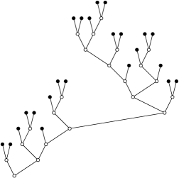
1. Introduction
The critical beta-splitting tree , introduced by Aldous [2], is a random recursive combinatorial structure, constructed in the following way. Assume that . We begin with the set . Let
| (1.1) |
denote the harmonic sum. The first split occurs between some and with probability
| (1.2) |
in which case separates into and . We call the critical beta-splitting distribution. See Figure 2.
The construction continues recursively, splitting and independently, etc., until only the singleton sets remain.
Finally, the tree is obtained as follows. Let denote the set of subsets of , determined by the splits in the above procedure. For each , a leaf is placed at height
The “” above accounts for the singleton set , which does not contribute to the height of .
An internal node is added to the tree, for each with . The two children of are and , where are the unique pair for which . There are internal nodes in total, one between each and . The first internal node is called the root of . The height is simply the graph distance (number of edges) between and . See Figure 1 for an example.
As discussed in [2], the tree is “critical” in the following sense. A tree could be constructed in a similar way, but with instead proportional to . The value in the above construction is of particular interest, since at this point typical heights switch from polynomial order to poly-logarithmic order .
1.1. Results
Amongst other results, Aldous and Pittel [3] recently proved a central limit theorem for , where is uniformly random in . In other words, is the height of a random leaf in .
Let
denote the Riemann zeta function.
Theorem 1 (Aldous and Pittel [3]).
As , we have that
is asymptotically normal.
1.2. Purpose
Our purpose is to give another proof of Theorem 1, along with a bound on the rate of convergence, see Theorem 3 below. We will use the contraction methods of Neininger and Rüschendorf [7, 8] (cf. Rösler [13, 14], Rachev and Rüschendorf [12] and Rösler and Rüschendorf [15]), together with the estimates for the mean and variance of obtained in [3], see (3) below.
We will also discuss, in Section 4.2 below, connections with a result of Iksanov, Marynych and Möhle [6], on collisions in the beta-coalescent.
1.3. Discussion
The limit theory in [7] was, in part, developed in response to work of Pittel [11], in which limit theorems are proved for various combinatorial quantities of interest (e.g., the independence number of a uniformly random labelled tree) with mean and variance that are close to linear.
The following line of reasoning is referred to as “Pittel’s principle” in [7, p. 379]. Indeed, in [11, p. 1260], the author states that:
For various global characteristics of large size combinatorial structures […] one can usually estimate the mean and the variance, and also obtain a recurrence for the generating function […]. As a heuristic principle based on our experience, we claim that such a characteristic is asymptotically normal if the mean and the variance are “nearly linear” […]. The technical reason is that in such a case the moment generating function […] of the normal distribution with the same two moments “almost” satisfies the recurrence.
A general theory is developed in [7], which, in particular, yields limit theorems in such situations (see [7, Corollary 5.2]). In fact, their results apply to a large family of random structures , which satisfy a distributional recurrence of the form (see [7, (1)])
| (1.3) |
As discussed in [7], such situations arise, e.g., in divide-and-conquer type algorithms. In this context, is called the toll function, associated with the “cost” of splitting into smaller, but similar subproblems.
Under certain conditions, a limit theorem can be proved for satisfying (1.3), via the so-called contraction method. Roughly speaking, this strategy aims to identify the limiting distribution of , by means of the fixed point equation
| (1.4) |
obtained by taking in (1.3). The normal distribution is associated with the situation that and .
See [7, Theorem 5.1 and Corollary 5.2] for their univariate results. See also [7, §5.4] for discussion on the multivariate case, and when is random, and potentially also .
The height of a random leaf in the critical beta-splitting tree satisfies a simple recurrence. Specifically, by (1.2), we have that
| (1.5) |
where
| (1.6) |
That being said, the results in [7] do not apply. The problem is that , , and that, as it turns out (see (3) below), the mean and variance of are of poly-logarithmic order. This leads to a trivial fixed point equation , which yields no information about .
However, the follow-up article [8], by the same authors, deals with this very situation, and it is these results that we will apply in the current article. Specifically, we will use Theorem 2.1 in [8]. In fact, this result does not apply as stated, but we will show that its proof can be suitably adapted.
We note that several applications of contraction methods are discussed in, e.g., [7, §5.2–5.3] and [8, §4–5]. In many cases, limit theorems follow quite easily using these techniques. We were introduced to them, while studying randomized importance sampling algorithms for perfect matchings [4] (cf. Neininger and Straub [9]).
1.4. Time-heights
In closing, let us mention that it is also natural to consider an alternative formation of , in which splitting events occur continuously in time. In [3], the authors analyze the case of exponential holding times on subsets, with rates on subsets of size . In this setting, a central limit theorem is proved for the time-height of a random leaf. Aldous [1] has given an alternative, probabilistic proof, via martingales.
A limit theorem for seems to be out of reach, however, by the methods in the current article, mainly due to the fact that has smaller variance, see (3) and (4.1) below. Therefore, it would appear that the critical beta-splitting tree provides an example of a model, at the borderline of what can be analyzed using current contraction techniques.
1.5. Acknowledgments
We thank David Aldous and Boris Pittel for inspiring conversations.
2. Contraction, with trivial fixed point
To begin, let us state the main result in [8, Theorem 2.1].
Suppose that a sequence of random variables satisfies
| (2.1) |
where and are independent, and takes values in . (In [8], can take values in , but we have no use for this.)
Let and .
As usual, denotes the -norm.
3. Proof of Theorem 1
We will use the following, remarkably precise, estimates in [3, Theorem 1.2]. Throughout this section, we let and . We have that
| (3.1) |
where
is the Euler–Mascheroni constant.
The reason Theorem 2 does not apply directly is that, by (1.1) and (1.6), we have that
| (3.2) |
We do, however, have the distributional recurrence (1.5). Hence, by (3) and (3), we have, in the notation of Theorem 2, that , , and . In particular, to see that , let us note that, by elementary arguments it can be shown, using (3) and (3), that
| (3.3) |
We will prove the following result, which, as we will see, follows by the proof of Theorem 2 (Theorem 2.1 in [8]), after a few adjustments.
Theorem 3.
Let be the height of a uniformly random leaf in the critical beta-splitting tree . Then
is asymptotically normal, where and . Furthermore, for any ,
where is a standard normal random variable.
In what follows, we will assume familiarity with the proof of Theorem 2.1 in [8], and the notation introduced therein. Since only a few changes are required, we will not explain the full proof here, but rather only discuss the places that need adjustment.
Proof.
We put , so that, by (3),
There are two main parts of the proof of [8, Theorem 2.1] that need attention. The first is the technical result [8, Lemma 3.1]. In fact, the proof of this result simplifies. Secondly, we will revisit the upper bound [8, (19)], as this estimate is used in the inductive proof of [8, Lemma 3.1].
Let us start with the second part. Recall that . We set , and let play the role of .
As noted above, . In particular, we simply have
We claim that the right hand side of [8, (23)] (and so also the left hand side of [8, (19)]) is . To see this, we first note, using (3.3), that . Similarly, it can be shown that . Next, we observe that, clearly, . Finally, we note, by similar arguments as (3.3), that
It follows that , and
Altogether, the right hand side of [8, (23)] is , as claimed.
Therefore, to the complete the proof, it remains only the prove the following analogue of the technical result in [8, Lemma 3.1].
Claim 4.
Let be as in (1.6). Suppose that nonnegative sequences and satisfy
| (3.4) |
and
| (3.5) |
Then, for all small , it follows that
To see this, we will follow the proof of [8, Lemma 3.1]. We can, in fact, make some simplifications in this special case. Using (1.6), (3) and (3.5), let and be such that and
for all .
Put
To prove the claim, we will show, by induction, that . By the choice of , there is nothing to prove for . On the other hand, for , by (3.4), the choice of , and the inductive hypothesis,
as required.
This finishes the proof, as the rest of the proof of Theorem 2.1 in [8] applies, without any further changes. ∎
4. Final remarks
4.1. Time-height
Recall, as discussed in Section 1.4 above, that is the time-height of the critical beta-splitting tree with exponential holding times. In [3, Theorem 1.1], it is shown that
| (4.1) |
Finer estimates are available, assuming a certain “-ansatz,” see [3, §2.2].
4.2. Collisions
Finally, as mentioned in Section 1.2 above, let us discuss the central limit theorem proved by in [6] for the number of collisions in the -coalescent. See, e.g., Pitman [10], Sagitov [16] and the survey by Gnedin, Iksanov and Marynych [5] for background.
In [6, (2)], there is a similar recurrence as (1.5) above. Also, Theorem 2 does not apply for similar reasons (compare (3) with [6, Remark 3.2]). To overcome this issue, an alternative, and more complicated, recurrence is derived [6, (14)], and then Theorem 2 is applied. However, the authors ask [6, Remark 1.6] if a more direct proof, using the simpler recursion [6, (2)], is possible.
References
- 1. D. Aldous, The critical beta-splitting random tree II: Overview and open problems, preprint available at https://arxiv.org/abs/2303.02529.
- 2. by same author, Probability distributions on cladograms, Random discrete structures (Minneapolis, MN, 1993), IMA Vol. Math. Appl., vol. 76, Springer, New York, 1996, pp. 1–18.
- 3. D. Aldous and B. Pittel, The critical beta-splitting random tree: Heights and related results, preprint available at https://arxiv.org/abs/2303.02529.
- 4. P. Diaconis and B. Kolesnik, Randomized sequential importance sampling for estimating the number of perfect matchings in bipartite graphs, Adv. in Appl. Math. 131 (2021), Paper No. 102247, 41.
- 5. A. Gnedin, A. Iksanov, and A. Marynych, -coalescents: a survey, J. Appl. Probab. 51A (2014), no. Celebrating 50 Years of The Applied Probability Trust, 23–40.
- 6. A. Iksanov, A. Marynych, and M. Möhle, On the number of collisions in -coalescents, Bernoulli 15 (2009), no. 3, 829–845.
- 7. R. Neininger and L. Rüschendorf, A general limit theorem for recursive algorithms and combinatorial structures, Ann. Appl. Probab. 14 (2004), no. 1, 378–418.
- 8. by same author, On the contraction method with degenerate limit equation, Ann. Probab. 32 (2004), no. 3B, 2838–2856.
- 9. R. Neininger and J. Straub, On the contraction method with reduced independence assumptions, 33rd International Conference on Probabilistic, Combinatorial and Asymptotic Methods for the Analysis of Algorithms, LIPIcs. Leibniz Int. Proc. Inform., vol. 225, Schloss Dagstuhl. Leibniz-Zent. Inform., Wadern, 2022, pp. Art. No. 14, 13.
- 10. J. Pitman, Coalescents with multiple collisions, Ann. Probab. 27 (1999), no. 4, 1870–1902.
- 11. B. Pittel, Normal convergence problem? Two moments and a recurrence may be the clues, Ann. Appl. Probab. 9 (1999), no. 4, 1260–1302.
- 12. S. T. Rachev and L. Rüschendorf, Probability metrics and recursive algorithms, Adv. in Appl. Probab. 27 (1995), no. 3, 770–799.
- 13. U. Rösler, A limit theorem for “Quicksort”, RAIRO Inform. Théor. Appl. 25 (1991), no. 1, 85–100.
- 14. by same author, A fixed point theorem for distributions, Stochastic Process. Appl. 42 (1992), no. 2, 195–214.
- 15. U. Rösler and L. Rüschendorf, The contraction method for recursive algorithms, vol. 29, 2001, Average-case analysis of algorithms (Princeton, NJ, 1998), pp. 3–33.
- 16. S. Sagitov, The general coalescent with asynchronous mergers of ancestral lines, J. Appl. Probab. 36 (1999), no. 4, 1116–1125.
- 17. V. M. Zolotarev, Approximation of the distributions of sums of independent random variables with values in infinite-dimensional spaces, Teor. Verojatnost. i Primenen. 21 (1976), no. 4, 741–758.
- 18. by same author, Ideal metrics in the problem of approximating the distributions of sums of independent random variables, Teor. Verojatnost. i Primenen. 22 (1977), no. 3, 449–465.