Instantons and multibananas: Relating elliptic genus and cohomological Donaldson-Thomas theory

Oliver Leigh oliverle@math.uio.no Dept. of Mathematics, The University of Oslo
Abstract.

In this article the cohomological Donaldson-Thomas theory of local multibanana threefolds is computed using Descombes’ hyperbolic localisation formula. The resulting expression is precisely given by the elliptic genus of the moduli space of framed instanton sheaves. As part of the proof, an infinite-wedge-space trace formula is computed for the elliptic genus of the moduli space of framed instanton sheaves.

The author was supported by the Research Council of Norway grant number 302277 - “Orthogonal gauge duality and non-commutative geometry”.

1. Introduction

1.1. Cohomological Donaldson-Thomas invariants

Numerical Donaldson-Thomas (DT) invariants are a mathematical count of BPS states; in particular supersymmetric bound states in type II string compactifications. They were originally developed to study compact Calabi-Yau threefolds, for which they contain important deformation-invariant information, and have since been studied in much more generality [Tho00, §3], [MNOP06b].

Let $Y$ be a (not necessarily proper) Calabi-Yau 3-fold over ${\mathbb{C}}$, and consider a curve class $\beta\in H_{2}(Y,{\mathbb{Z}})$ and an integer $n\in{\mathbb{Z}}$. The numerical DT invariant $\mathsf{DT}_{\beta,n}(Y)$ is computed by considering the Hilbert scheme

$$\operatorname{Hilb}^{{}_{\beta,n}}(Y):=\{Z\subset Y\leavevmode\nobreak\ \leavevmode\nobreak\ |\leavevmode\nobreak\ \,[Z]=\beta\mbox{ and }\chi({\mathcal{O}}_{Z})=n\}.$$

The invariant $\mathsf{DT}_{\beta,n}(Y)$ is given by a weighted Euler characteristic of $\operatorname{Hilb}^{{}_{\beta,n}}(Y)$ [Beh09] or, equivalently if $Y$ is proper, a virtual fundamental class of $\operatorname{Hilb}^{{}_{\beta,n}}(Y)$ [Tho00].

In recent years, the research group of Joyce has developed a rigorous general theory of cohomological DT invariants in [Joy15, BBJ19, BBD+15, BBBBJ15], based on ideas due to Kontsevich and Soibelman in [KS08, KS11], and Dimca and Szendrői in [DS09] (see also [Dav17, DM20], and for an excellent introduction to the field [Sze16]). Cohomological DT invariants provide more nuanced information, at the expense of deformation invariance (see [Sze16, §8.1] for a discussion), and they are valued in the abelian category of monodromic mixed Hodge structures, ${\mathrm{MMHS}}=\operatorname{\mathrm{MMHM}}(\operatorname{Spec}{\mathbb{C}})$.

The key result needed to define cohomological DT invariants in the present article is:

Theorem 1.1 ([BBD+15, Cor. 6.12] and [BD21]).

Let $\phi:{\mathcal{E}}^{\bullet}\rightarrow L^{\bullet}_{\operatorname{Hilb}^{{}_{\beta,n}}(Y)}$ be the natural symmetric obstruction theory of Thomas [Tho00, Thm. 3.30]. For a given choice of square root $\det({\mathcal{E}}^{\bullet})^{1/2}$ there is a monodromic mixed hodge module $\mathcal{DT}^{\bullet}_{Y,\beta,n}\in\operatorname{\mathrm{MMHM}}(\operatorname{Hilb}^{{}_{\beta,n}}(Y))$, which is unique up to canonical isomorphism, satisfying:

  • If $\operatorname{Hilb}^{{}_{\beta,n}}(Y)$ is locally modelled by the critical locus of a regular function $f:U\rightarrow{\mathbb{C}}$ on a smooth ${\mathbb{C}}$-scheme $U$, then $\mathcal{DT}^{\bullet}_{Y,\beta,n}$ is locally modelled by $\mathcal{HV}^{\bullet}_{U,f}$, the monodromic mixed Hodge module lift of the perverse sheaf of vanishing cycles of $(U,f)$.

Remark 1.2.

The results of [BBD+15] apply to more general spaces than those given in Theorem 1.1. We have restricted to the case at hand in order to simplify the exposition.

Remark 1.3.

Nekrasov and Okounkov show in [NO16, §6] (see also [Arb21, Prop. 2.1]) that a choice of square root $\det({\mathcal{E}}^{\bullet})^{1/2}$ for Theorem 1.1 always exists.

We call $\mathcal{DT}^{\bullet}_{Y,\beta,n}$ the DT mixed hodge module. As discussed in [BBD+15, Rem. 2.22], the hypercohomology of a monodromic mixed Hodge module also has the structure of a monodromic mixed Hodge structure. Hence, using the monodromic mixed Hodge module from Theorem 1.1 one can define cohomological DT invariants as follows:

Definition 1.4.

The cohomological Donaldson-Thomas invariants are defined by

$$\mathbb{DT}_{\beta,n}(Y):={\mathbb{H}}^{\bullet}\left(\mathcal{DT}^{\bullet}_{Y,\beta,n}\right)\in K({\mathrm{MMHS}})$$

where ${\mathbb{H}}^{\bullet}(-)$ is compactly supported hypercohomology.

Remark 1.5.

As discussed in [Beh09] and [BBD+15, Remark 6.14], the numerical DT invariant can be recovered from the cohomological DT invariant by

$$\mathsf{DT}_{\beta,n}(X)=\sum_{k\in{\mathbb{Z}}}(-1)^{k}\dim{\mathbb{H}}^{k}\left(\mathcal{DT}^{\bullet}_{Y,\beta,n}\right).$$

Similar to the case of numerical DT invariants, one can assemble the cohomological DT invariants into a partition function

$$Z^{\mathbb{DT}}(Y):=\sum_{\beta\in H_{2}(Y,{\mathbb{Z}})}\sum_{n\in{\mathbb{Z}}}\leavevmode\nobreak\ \mathbb{DT}_{\beta,n}(Y)\,Q^{\beta}\,q^{n},$$

where $Z^{\mathbb{DT}}(Y)$ is an element of $K({\mathrm{MMHS}})[q^{-1}][[q,Q]]$. Here an effective basis $\beta_{1},\ldots,\beta_{n}$ of $H_{2}(Y,{\mathbb{Z}})$ has been chosen i.e. if $\beta$ is effective then $\beta=\sum d_{i}\beta_{i}$ for $d_{i}\geq 0$, and the convention $Q^{\beta}=\prod Q_{i}^{d_{i}\beta_{i}}$ has been used.

The above partition function is very hard to compute. Indeed, even for the easier numerical DT version, there is no complete computation for any proper Calabi-Yau threefold with trivial first Betti number. The case is worse for cohomological DT theory, but the recent hyperbolic localisation formula of [Des22b] (discussed more in Section 2.1) has provided a powerful tool for calculations. In the present article, we use this tool to compute the cohomological DT theory of local multibanana Calabi-Yau threefolds.

Most previous calculations in this area have been from the view-point of motivic DT invariants, introduced in [KS08]. These take values in a Grothendieck ring of varieties, but can be converted to cohomological DT theory as described in [KS11, §7.10] and [Dav19, App. A]. From this point of view, the partition function $Z^{\mathbb{DT}}(Y)$ has been computed for local curves in [MMNS12, MN15, DM17, Des22a] (see [MP20, §5] for a review), and the invariants for the one-loop quiver with potential were calculated in [DM15]. The theory relating to some local surfaces has also been computed in [BMP21, MP20, Des22a].

1.2. Local multibanana threefolds

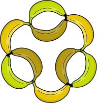
Local multibanana threefolds are examples of non-singular toric varieties without a finite type fan. Their name is derived from the shape of a curve configuration which is discussed below and depicted in Figure 2.

Following Kanazawa and Lau [KL19, §5], for $i,j\in{\mathbb{N}}$, one can construct the local multibanana threefold of type $(i,j)$ as a quotient of a toric threefold with a non-finite-type fan. We can construct this fan by first considering the lines $\mathsf{L}_{f,m}:=\big{\{}p\in{\mathbb{C}}^{3}\,|\,f(p)=m,z=1\big{\}}$ and the tiling of $\{(x,y,1)\,|\,x,y\in{\mathbb{C}}\}$ given by the collection:

$$\big{\{}\mathsf{L}_{x,l}\big{\}}_{l\in{\mathbb{Z}}}\cup\big{\{}\mathsf{L}_{y,m}\big{\}}_{m\in{\mathbb{Z}}}\cup\big{\{}\mathsf{L}_{x-y,n}\big{\}}_{n\in{\mathbb{Z}}}.$$

This tiling also defines a non-finite-type fan $F$ by taking the all cones over the proper faces of the tiling. This is depicted in Figure 1 below.

$A_{0}$ $C_{0}$ $B_{1}$ $B_{0}$ $A_{0}$ $C_{1}$ $A_{1}$ $B_{2}$ $B_{1}$ $A_{1}$ $C_{2}$ $A_{2}$ $B_{0}$ $B_{2}$ $A_{2}$ $C_{0}$ $B_{0}$ $C_{1}$ $C_{0}$ $A_{2}$ $C_{2}$ $C_{1}$ $C_{0}$ $C_{2}$ $A_{1}$ $B_{0}$

Figure 1. On the left is part of the non-finite type toric fan of ${\mathcal{X}}$, and on the right is the web diagram of the local multibanana threefold $X_{(3,1)}$.

Now, take the threefold ${\mathcal{X}}$ defined by $F$ and observe that ${\mathcal{X}}$ has a free $i{\mathbb{Z}}\oplus j{\mathbb{Z}}$-action coming from translations of $F$. We define the local multibanana threefold of type $(i,j)$ by

$$X_{(i,j)}:={\mathcal{X}}/i{\mathbb{Z}}\oplus j{\mathbb{Z}}.$$

The focus of this article is $X_{(r,1)}$, and for convenience, we restrict to this space from now on. $X_{(r,1)}$ has a natural ${\mathbb{T}}^{2}$ action and, as explained in [KL19, §5.1], the ${\mathbb{T}}^{2}$-fixed curves are unions of $(-1,-1)$-rational curves corresponding to 2-dimensional sub-cones. Following Bryan [Bry21], we call these the banana curves and label them by their sub-cones

$\displaystyle A_{k}$ $\displaystyle\sim\mathbb{R}_{\geq 0}\mathrm{Conv}\big{(}\{(0,k,1),(0,k+1,1)\}\big{)},$
$\displaystyle B_{k}$ $\displaystyle\sim\mathbb{R}_{\geq 0}\mathrm{Conv}\big{(}\{(k+1,k,1),(k,k+1,1)\}\big{)},$
$\displaystyle C_{k}$ $\displaystyle\sim\mathbb{R}_{\geq 0}\mathrm{Conv}\big{(}\{(k,0,1),(k+1,0,1)\}\big{)}.$

As pointed out in [KL19, §5.1], the banana curves have the relations

$$A_{k}+B_{k}=A_{k}+B_{k+1}\hskip 28.45274pt\mbox{and}\hskip 28.45274ptB_{k}+C_{K}=B_{k+1}+C_{K+1}$$

in $H_{2}\big{(}X_{(r,1)},{\mathbb{Z}}\big{)}$, and hence the banana curves form the r+2 classes

$$A_{0},\ldots,A_{r-1},\hskip 28.45274ptB=B_{0},\ldots,B_{r-1},\hskip 28.45274pt\mbox{and}\hskip 28.45274ptC=C_{0},\ldots,C_{r-1}.$$

Moreover, by [KL19, Lem. 5.3] these classes give an effective basis for $H_{2}\big{(}X_{(r,1)},{\mathbb{Z}}\big{)}$.

The banana curves are either disjoint or meet as the coordinate axis in a copy of ${\mathbb{C}}^{3}$. This is depicted in the web diagram of Figure 1 and the banana diagrams in Figure 2. We call the union of the banana curves a banana configuration. Interestingly, the mirror symmetry of Banana configurations (called perverse curves) was previously studied by Ruddat in [Rud17].

$A_{0}$ $A_{1}$ $A_{2}$ $B_{0}$ $C_{0}$ $B_{1}$ $C_{1}$ $B_{2}$ $C_{2}$           Refer to caption

Figure 2. Depictions of the banana configurations. (Banana image from: Vecteezy.com)

1.3. Enumerative geometry of local multibanana threefolds

The enumerative geometry of banana threefolds was first studied by Bryan in [Bry21]. He considered an elliptically-fibred proper Calabi-Yau threefold $X_{\mathsf{ban}}$ containing subschemes locally isomorphic to $X_{(1,1)}$, then computes the numerical DT partition function for the banana-curve sublattice. We give a cohomological generalisation of the local version of Bryan’s formula in Corollary 1.11.

Bryan’s results were extended by the author in [Lei20], by also considering the section of the elliptic fibration. In forthcoming work, Bryan and Pietromonaco consider related quotient spaces called banana nano-manifolds in [BP24]. In another direction, Katz’s genus 0 Gopakumar-Vafa partition function of $X_{\mathsf{ban}}$ for the banana-curve sublattice was partially computed in [Mor22]. This calculation was extended to $X_{(r,1)}$ and $X_{(2,2)}$ in [Mor21].

From the discussion in Section 1.2 we know $A_{0},\ldots,A_{r-1},B,C$ is an effective basis for $H_{2}(X_{(r,1)},{\mathbb{Z}})$, and denote the corresponding formal variables by $Q_{A_{0}},\ldots,Q_{A_{r-1}},Q_{B},Q_{C}$. We can also define a restricted partition function $Z^{\mathbb{DT}}_{c}(X_{(r,1)})$ by

$$Z^{\mathbb{DT}}\big{(}X_{(r,1)}\big{)}=\sum_{c\geq 0}\,Z^{\mathbb{DT}}_{c}\big{(}X_{(r,1)}\big{)}\,Q_{C}^{c}.$$

The main result of this article is the following explicit formula for this partition function.

Theorem 1.6 (Main Theorem).

Let ${\mathbb{L}}^{1/2}$ be the monodromic mixed hodge module of ${\mathbb{C}}\rightarrow{\mathbb{C}};z\mapsto z^{2}$ as detailed in [DM20, p. 803], and let ${\mathbb{L}}^{-1/2}$ be its formal inverse. Define

$$\Theta_{p,y}(t):=\prod_{n>0}\dfrac{(1-y\,p^{n-1}t)}{(1-p^{n-1}t)}\dfrac{(1-y^{-1}p^{n}t^{-1})}{(1-p^{n}t^{-1})},$$

the generalised MacMahon function $M(u;v,w):=\prod_{k,l>0}(1-u\,v^{k}\,w^{l})^{-1},$ and for a 2D partition Y with $(i,j)\in Y$ the arm and leg lengths $a_{Y}(i,j):=Y_{i}-j$ and $l_{Y}(i,j):=(Y^{T})_{j}-i$.

Then, for any choice of orientation, we have that $Z^{\mathbb{DT}}_{c}\big{(}X_{(r,1)}\big{)}$ is equal to the expression

$\displaystyle{\mathcal{Z}}_{0}^{\mathbb{DT}}\cdot Q_{B}^{(1-r)c}\!\!\!\sum_{\scriptsize\begin{array}[]{c}\gamma_{0},\ldots,\gamma_{r-1}\\ s.t.\sum\gamma_{i}=c\end{array}}\!\!\!\!\!\big{(}-u^{-\frac{1}{2}}{v}^{\frac{1}{2}}\big{)}^{rc}\prod_{i,j=0}^{r-1}\,\prod_{x\in\gamma_{i}}\,\Theta_{\mathtt{e}_{r-1},-u^{1/2}v^{-1/2}Q_{B}}\!\left(\dfrac{\mathtt{e}_{i}}{\mathtt{e}_{j}}u^{-a_{\gamma_{i}}(x)-1}v^{-l_{\gamma_{j}}(x)}\right)$
$\displaystyle\hskip 180.90024pt\prod_{z\in\gamma_{j}}\,\Theta_{\mathtt{e}_{r-1},-u^{1/2}v^{-1/2}Q_{B}}\!\left(\dfrac{\mathtt{e}_{i}}{\mathtt{e}_{j}}u^{a_{\gamma_{j}}(z)}v^{l_{\gamma_{i}}(z)+1}\right)$

where $u:=-q\,{\mathbb{L}}^{1/2}$, $v:=-q\,{\mathbb{L}}^{-1/2}$ and $\mathtt{e}_{i}:=\prod_{j=0}^{i}Q_{A_{i}}Q_{B}$, and ${\mathcal{Z}}_{0}^{\mathbb{DT}}$ is given by the expression

$\displaystyle\leavevmode\nobreak\ M(v^{-1};u,v)^{r}\cdot\prod_{0\leq i<j\leq r-1}\frac{M\big{(}\mathtt{e}_{i}\,\mathtt{e}_{j}^{-1}v^{-1};u,v\big{)}}{M\big{(}\mathtt{e}_{j}\,\mathtt{e}_{i}^{-1}u^{-1};u,v\big{)}}\frac{M\big{(}-Q_{B}\,\mathtt{e}_{j}\,\mathtt{e}_{i}^{-1}(uv)^{-\frac{1}{2}};u,v\big{)}}{M\big{(}-Q_{B}^{-1}\mathtt{e}_{i}\,\mathtt{e}_{j}^{-1}(uv)^{-\frac{1}{2}};u,v\big{)}}$
$\displaystyle\leavevmode\nobreak\ \cdot\prod_{N>0}\frac{1}{1-e_{r-1}^{N}}\prod_{i,j=0}^{r-1}\frac{M\big{(}\mathtt{e}_{r-1}^{N-1}\mathtt{e}_{i}\,\mathtt{e}_{j}^{-1}u^{-1};u,v\big{)}}{M\big{(}-Q_{B}\,\mathtt{e}_{r-1}^{N-1}\mathtt{e}_{i}\,\mathtt{e}_{j}^{-1}(uv)^{-\frac{1}{2}};u,v\big{)}}\frac{M\big{(}\mathtt{e}_{r-1}^{N}\mathtt{e}_{i}\,\mathtt{e}_{j}^{-1}v^{-1};u,v\big{)}}{M\big{(}-Q_{B}^{-1}\mathtt{e}_{r-1}^{N}\mathtt{e}_{i}\,\mathtt{e}_{j}^{-1}(uv)^{-\frac{1}{2}};u,v\big{)}}.$
Remark 1.7.

Another interesting refinement of DT invariants is given by the K-theoretic DT invariants of [NO16] (see also [Arb21, Arb22]). In the case when $Y$ is proper, these are predicted to be the $\chi_{y}$-genus of the cohomological DT invariants. However, in the case where $Y$ is non-proper, there is a discrepancy. An example is when $Y={\mathbb{C}}^{3}$ and $\beta=0$ as computed motivically by [BBS13] and K-theoretically by [NO16, §8.3]. This relationship is discussed in [Des22a, §4.4 and §5.1].

Another discrepancy is for $X_{(r,1)}$. K-theoretic DT invariants use a refinement parameter arising from the equivariant weight of the canonical bundle. However, since ${\mathbb{T}}^{2}$ is a Calabi-Yau torus on $X_{(r,1)}$, this refinement parameter is $1$, and no extra information is obtained in this case.

1.4. Elliptic genus of the moduli space of framed instanton sheaves

Theorem 1.6 has a striking relationship with the elliptic genus of framed instanton sheaves, which we will discuss in this section. We first recall the definition and some key properties of the moduli space of framed instanton sheaves on ${\mathbb{P}}^{2}$.

Definition-Theorem 1.8 ([NY05]).

The moduli space of frame instanton sheaves on ${\mathbb{P}}^{2}$ $\mathcal{M}(r,N)$ is the nonsingular scheme of dimension $2rN$ parameterising pairs

$$\Big{(}\,E,\,\Phi:E|_{\ell_{\infty}}\overset{\sim}{\longrightarrow}{\mathcal{O}}_{\ell_{\infty}}^{\oplus r}\,\Big{)}$$

where $E$ is a rank $r$ torsion free sheaf on ${\mathbb{P}}^{2}$ with $\left<c_{2}(E),[{\mathbb{P}}^{2}]\right>=n$ and that is locally free in a neighborhood of $\ell_{\infty}:=\{[0:z_{1}:z_{2}]\}$, and $\Phi$ is an isomorphism. It has the following properties:

  1. (i)

    $\mathcal{M}(r,N)$ is acted upon by a $2+r$-dimensional torus, ${\mathbb{E}}^{2+r}$, with associated characters $t_{1},t_{2},e_{0},\ldots,e_{r-1}$.

  2. (ii)

    The fixed points $\mathcal{M}(r,N)^{{\mathbb{E}}^{2+r}}$ are isolated and are in bijection to the set of $r$-tuples of Young diagrams $\bm{Y}=(Y_{1},\ldots,Y_{r})$ satisfying $\sum_{i=1}^{r}\lvert Y_{i}\rvert=N$.

  3. (iii)

    For a fixed point $\bm{Y}$, the equivariant $K$-theory class of the restricted tangent bundle $T_{\mathcal{M}(r,N)}|_{\bm{Y}}$ is given by

    $$\sum_{a,b=0}^{r-1}e_{b}\,e_{a}^{-1}\cdot\left(\sum_{s\in Y_{a}}\left(t_{1}^{-l_{Y_{b}}(s)}t_{2}^{a_{Y_{a}}(s)+1}\right)+\sum_{t\in Y_{b}}\left(t_{1}^{l_{Y_{a}}(t)+1}t_{2}^{-a_{Y_{b}}(t)}\right)\right).$$

Recall that elliptic genus can be defined by taking the Chern roots $L_{i}$ of a tangent bundle and considering the multiplicative class

$\displaystyle\operatorname{\mathcal{E}\!\mathit{ll}}_{u,y}(L)\leavevmode\nobreak\ :=\leavevmode\nobreak\ c_{1}(L)\frac{\theta_{1}(u,y\operatorname{ch}(-L))}{\theta_{1}(u,\operatorname{ch}(-L))}\leavevmode\nobreak\ =\leavevmode\nobreak\ \frac{c_{1}(L)}{y^{\frac{1}{2}}}\cdot\Theta_{u,y}\big{(}c_{1}(-L)\big{)}.$

Now, combining Definition-Theorem 1.8 with Theorem 1.6 we have the following corollary.

Corollary 1.9 (Partition function as elliptic genus).

Considering ${\mathbb{L}}^{1/2}$ as a formal variable, we have the relationship

$$\frac{Z^{\mathbb{DT}}_{c}\big{(}X_{(r,1)}\big{)}}{Q_{B}^{c}\cdot{\mathcal{Z}}_{0}^{\mathbb{DT}}}=\mathrm{Ell}_{\mathtt{e}_{r-1},-{\mathbb{L}}^{\frac{1}{2}}Q_{B}}\left(\mathcal{M}(r,c);\mathtt{e}_{0},\ldots,\mathtt{e}_{r-1},{\mathbb{L}}^{\frac{1}{2}}q^{-1},{\mathbb{L}}^{\frac{1}{2}}q\right)$$

where $\mathtt{e}_{i}:=\prod_{j=0}^{i}Q_{A_{i}}Q_{B}$ and ${\mathcal{Z}}_{0}^{\mathbb{DT}}$ is given in Theorem 1.6.

Remark 1.10.

As part of the proof of Theorem 1.6 and Corollary 1.9 we obtain a natural expression for

$$\mathrm{Ell}_{u,y}\left(\mathcal{M}(r,N);e_{0},\ldots,e_{r-1},t_{1},t_{2}\right)$$

as a trace of vertex operators of Okounkov [Oko01] (see also [OR07, You10, BKY18]). The expression is given in Corollary 3.6. It is hoped that this will be useful in extending the $\chi_{y}$ Vafa-Witten Blowup formula of [KLT22] to elliptic genus.

The relationship between DT theory of banana threefolds and elliptic genus was first observed by Bryan in [Bry21], where it was observed that the numerical Donaldson-Thomas partition function for the local banana threefold $(r=1)$ was determined by the equivariant elliptic genus of the Hilbert scheme of points on ${\mathbb{C}}^{2}$, where ${\mathbb{C}}^{*}$ acts diagonally.

Theorem 1.6 extends this result in two ways:

  1. (i)

    For $r=1$ the cohomological DT partition function is determined by the equivariant elliptic genus of the Hilbert scheme of points on ${\mathbb{C}}^{2}$ for the larger $({\mathbb{C}}^{*})^{2}$ torus.

  2. (ii)

    For $r>1$ the cohomological DT partition function is determined by the equivariant elliptic genus of the moduli space of framed instanton sheaves on ${\mathbb{P}}^{2}$.

In the $r=1$ case we can follow Bryan [Bry21] and use Waelder’s analogue of the DMVV formula [Wae08, Thm. 12] to obtain an infinite product formula.

Corollary 1.11 (Product formula for the banana case, $r=1$).

For $r=1$ the full partition function is

$\displaystyle Z^{\mathbb{DT}}=\leavevmode\nobreak$ $\displaystyle\prod_{d_{A},d_{B}d_{C}\geq 0}\!\prod_{\scriptsize\begin{array}[]{c}\bm{k}=(k_{1},k_{2})\in(\frac{1}{2}{\mathbb{Z}})^{2}\\ \mbox{s.t. $\bm{k}\neq\bm{0}$ if $\bm{d}=\bm{0}$ }\end{array}}\!\!\!\!\Big{(}1-(-Q_{A_{0}})^{d_{A}}(-Q_{B})^{d_{B}}(-Q_{C})^{d_{C}}v^{-k_{1}}u^{k_{2}}\Big{)}^{-b(\|\bm{d}\|,k_{1},k_{2})}.$

where $\bm{d}:=(d_{A},d_{B},d_{C})$, $\|\bm{d}\|:=2d_{A}d_{B}+2d_{A}d_{C}+2d_{B}d_{C}-d_{A}^{2}-d_{B}^{2}-d_{C}^{2}$ and $b(a,k_{1},k_{2})$ is defined by the expansion as a Laurent series in $p,y,t_{1}^{{}_{-1/2}},t_{2}^{{}_{1/2}}$ of

$$\sum_{a\geq-1}\sum_{k_{1},k_{2}\in\frac{1}{2}{\mathbb{Z}}}b(a,k_{1},k_{2})Q^{a}t_{1}^{-k_{1}}t_{2}^{k_{2}}=\frac{\sum_{k\in{\mathbb{Z}}}Q^{k^{2}}\big{(}-(t_{1}t_{2})^{\frac{1}{2}}\big{)}^{k}}{\left(\sum_{k\in{\mathbb{Z}}+\frac{1}{2}}Q^{2k^{2}}(-t_{1})^{-k}\right)\left(\sum_{k\in{\mathbb{Z}}+\frac{1}{2}}Q^{2k^{2}}(-t_{2})^{k}\right)}$$
Remark 1.12.

It is unclear whether such a product formula exists in the general case. On the positive side: The existence of a product formula is equivalent to the existence of the associated Gopakumar-Vafa-invariant formula (see [Bry21, Def.-Thm. A.13] for more details).

Given the link with elliptic genus of $\mathcal{M}(r,n)$, one would hope that such a product formula extends to the elliptic genus generating function as well. In the non-framed case, the moduli space of rank 2 stable sheaves on a surface has been shown to have product formula by Göttsche and Kool in [GK19]. A product formula for general rank would be extremely useful in extending the $\chi_{y}$ Vafa-Witten blowup formula of [KLT22] to elliptic genus, and similarly extending a forthcoming result of Arbesfeld, Kool and Laarakker [AKL24].

1.5. Structure of the article

The article is structured as follows:

  1. -

    In Section 2 we compute the partition function in terms of the refined topological vertex. The method is to combine Descombes’ hyperbolic localisation formula [Des22b, Thm. 1.1] with the K-theoretic computational results of Arbesfeld [Arb21].

  2. -

    In Section 3 we compute the formulas in Theorem 1.6 and Corollary 1.11 using Okounkov’s vertex operators [Oko01]. We also obtain a trace formula for the elliptic genus of the moduli space of framed instanton sheaves on ${\mathbb{P}}^{2}$ (given in Corollary 3.6).

2. Computation of cohomological DT theory

2.1. Descombes’ hyperbolic localisation formula

Cohomological DT invariants are very hard to compute, and the torus localisation techniques used in numerical DT theory [GP99, CKL17] are insufficient in the cohomological setting. It was suggested by Szendrői [Sze16, §8.4] that the ideas of Braden [Bra03] for hyperbolic localisation on intersection cohomological could be applied to cohomological DT theory as well. Hyperbolic localisation for cohomological DT invariants was proved by Descombes in [Des22b], and will be the basis for the results of this article.

Hyperbolic localisation applies in the setting of an algebraic space $X$ with the action of a one dimensional torus ${\mathbb{C}}^{*}$. The underlying concept of hyperbolic localisation is the decomposition of Białynicki-Birula [BB73] (extended from smooth varieties by [Bra03, Dri13]). In this setting we consider the ${\mathbb{C}}^{*}$-fixed space $X_{0}$ and also the attracting variety $X^{+}$, which is the subset of points $x\in X$ such that $\lim_{t\rightarrow 0}t\cdot x$ exists. We then consider the hyperbolic localization diagram as in [Bra03], [Dri13] and [Ric19]:

(2.1) ${X}$ ${X^{+}}$ ${X^{{\mathbb{C}}^{*}}}$ $\scriptstyle{\eta}$ $\scriptstyle{p}$

Here $\eta$ is the inclusion and $p$ is the natural morphism. The functor $p_{!}\eta^{*}$ is called the hyperbolic localization functor.

To apply hyperbolic localisation in the setting of this article, we consider a Calabi-Yau threefold with a ${\mathbb{C}}^{*}$-CY-action (i.e. locally the weights $(w_{1},w_{2},w_{3})$ have $w_{1}+w_{2}+w_{3}=0$), and observe that this action extends to one on $\operatorname{Hilb}_{\beta,n}(Y)$. The ${\mathbb{C}}^{*}$-action is compatible with the obstruction theory of [Tho00, Thm. 3.30] and we obtain a ${\mathbb{C}}^{*}$-equivariant perfect obstruction theory $\phi:{\mathcal{E}}^{\bullet}\rightarrow L^{\bullet}_{\operatorname{Hilb}_{\beta,n}(Y)}$. The ${\mathbb{C}}^{*}$-fixed locus can then be decomposed into connected components

$$\operatorname{Hilb}_{\beta,n}(Y)^{{\mathbb{C}}^{*}}=\bigsqcup_{\lambda\in\Lambda}P_{\lambda}.$$

In this article we focus on the case where each $P_{\lambda}$ is an isolated and reduced point. In this case

$$\mathcal{H}^{0}({\mathcal{E}}^{\bullet})^{\vee}\cong{\mathrm{Def}}_{P_{\lambda}},$$

and we define the index at $P_{\lambda}$ to be

$${\mathrm{Ind}}_{P_{\lambda}}:=\#\{\mbox{Positve ${\mathbb{C}}^{*}$-weights of ${\mathrm{Def}}_{P_{\lambda}}$}\}-\#\{\mbox{Negative ${\mathbb{C}}^{*}$-weights of ${\mathrm{Def}}_{P_{\lambda}}$}\}.$$

Now, Descombes’ hyperbolic localisation formula is given by the following theorem.

Theorem 2.1 ([Des22b, Thm. 1.1]).

Suppose $\operatorname{Hilb}_{\beta,n}(Y)^{{\mathbb{C}}^{*}}$ is a finite collection of reduced points. Then there is an isomorphism of monodromic mixed hodge modules

$$p_{!}\eta^{*}\mathcal{DT}^{\bullet}_{Y,\beta,n}\cong\bigoplus_{\lambda\in\Lambda}{\mathbb{L}}^{\frac{1}{2}{\mathrm{Ind}}_{\lambda}}.$$
Remark 2.2.

In [Des22b, Thm. 1.1], the hyperbolic localisation formula is given in more generality. In particular, the condition on the fixed loci is not needed. In general, each fixed loci would have an associated monodromic mixed hodge module (of the form given in Theorem 1.1) appearing on the right hand side of the formula. In the case of isolated smooth fixed points, we have used that this monodromic mixed hodge module is simply ${\mathbb{Q}}$ as described in [DM20, Eg. 2.11].

2.2. Analysis of the torus fixed locus

Analysis of the ${\mathbb{T}}^{2}$-fixed subschemes of $X_{(1,1)}$ was carried out by Bryan in [Bry21, §4.8] using toric techniques detailed in [MNOP06a] and [BCY12, §3 and App. B]. Essentially, a torus-invariant subscheme is determined by combinatorial data associated to its web diagram. The data involves a 2D partition for each edge and for each vertex, a 3D partition asymptotic to the the 2D partitions of the incident edges.

The analysis of the ${\mathbb{T}}^{2}$-fixed subschemes of $X_{(r,1)}$ is essentially the same as for $X_{(1,1)}$. The difference is seen by comparing [Bry21, Fig. 4] with the web diagram in Figure 1. Namely, the ${\mathbb{T}}^{2}$-fixed locus of $X_{(r,1)}$ has $2r$ vertices and $3r$ edges. We then arrive at the following lemma.

Lemma 2.3 (${\mathbb{T}}^{2}$-Fixed points).

For a curve class $\beta=\sum a_{i}\cdot A_{i}+b\cdot B+c\cdot C$ the fixed points of $\operatorname{Hilb}^{n,\beta}(Y)$ are indexed by the collection $\Lambda$ of tuples

$$\lambda=(\bm{\alpha},\bm{\beta},\bm{\gamma};\bm{\pi},\bm{\eta})$$

such that

  1. (i)

    $\bm{\alpha}=(\alpha_{0},\ldots,\alpha_{r-1})$ where $\alpha_{i}$ is a 2D partition with $|\alpha_{i}|=a_{i}$,

  2. (ii)

    $\bm{\beta}=(\beta_{0},\ldots,\beta_{r-1})$ where $\beta_{i}$ is a 2D partition with $\sum|\beta_{i}|=b$,

  3. (iii)

    $\bm{\gamma}=(\gamma_{0},\ldots,\gamma_{r-1})$ where $\gamma_{i}$ is a 2D partition with $\sum|\gamma_{i}|=c$,

  4. (iv)

    $\bm{\pi}=(\pi_{0},\ldots,\pi_{r-1})$ where $\pi_{i}$ is a 3D-partition asymptotic to $(\alpha_{i},\beta_{i},\gamma_{i})$,

  5. (v)

    $\bm{\eta}=(\eta_{0},\ldots,\eta_{r-1})$ where $\eta_{i}$ is a 3D-partition asymptotic to $(\alpha^{\prime}_{i-1},\beta^{\prime}_{i},\gamma^{\prime}_{i})$,

and

(2.2) $\displaystyle n=\frac{1}{2}\sum_{i}\Big{(}2|\pi_{i}|+2|\eta_{i}|+\|\alpha_{i}\|^{2}+\|\alpha^{\prime}_{i}\|^{2}+\|\beta_{i}\|^{2}+\|\beta^{\prime}_{i}\|^{2}+\|\gamma_{i}\|^{2}+\|\gamma^{\prime}_{i}\|^{2}\Big{)}.$

Here for a 2D partition $\mu$ we have used $\|\mu\|^{2}=\sum\mu_{i}^{2}$ and for a 3D-partition $\nu$ we have used the renormalised volume [ORV06, BKY18]:

$$|\nu|:=\sum_{\raisebox{-1.12003pt}{\mbox{\mancube}}\,\in\nu}\Big{(}1-\#\,\big{\{}\mbox{legs of $\nu$ containing \mancube}\big{\}}\Big{)}.$$

$A_{i}$ $C_{i}$ $B_{i+1}$ $B_{i}$ $A_{i}$ $C_{i+1}$ $B_{i}$ $C_{i+1}$ $C_{i}$ $A_{i-1}$ $A_{i+1}$ $B_{i}$ $w_{2}$ $w_{1}$ $-w_{2}$ $w_{2}+w_{1}$ $-w_{2}-w_{1}$ $w_{1}$ $-w_{2}$ $-w_{1}$ $w_{2}$ $-w_{2}-w_{1}$ $w_{2}+w_{1}$ $-w_{1}$ $-w_{2}-w_{1}$ $-w_{1}$ $w_{2}$ $w_{2}+w_{1}$ $w_{1}$ $-w_{2}$

Figure 3. A depiction of how the Calabi-Torus ${\mathbb{T}}^{2}$ acts on $X_{(r,1)}$.

To apply the hyperbolic localisation formula, we may choose a ${\mathbb{C}}^{*}$-subtorus of ${\mathbb{T}}^{2}$ given by weights $(w_{1},w_{w})$ and with character denoted by $t$. The local description of this is given in Figure 3. The (general) hyperbolic localisation formula is unaffected by the choice of ${\mathbb{C}}^{*}$-subtorus and we choose a subtorus such that

$$\operatorname{Hilb}^{\beta,n}\big{(}X_{(r,1)}\big{)}^{{\mathbb{C}}^{*}}=\operatorname{Hilb}^{\beta,n}\big{(}X_{(r,1)}\big{)}^{{\mathbb{T}}^{2}}$$

so that we can apply Theorem 2.1. (The condition required is that $w_{1}\neq n\cdot w_{2}$ for any $n\in{\mathbb{Z}}$.) We will use the results of [Arb21, §4], where a choice of ${\mathbb{C}}^{*}$-subtorus is called a slope. Indeed, we assume for later convenience that $w_{1}>>w_{2}>0$ in which case we are using a preferred slope of [Arb21].

Proposition 2.4.

$Hilb^{\beta,n}(X_{(r,1)})$ is equal to its attracting locus, $Hilb^{\beta,n}(X_{(r,1)})^{+}$.

Proof.

This follows because the web diagram of $X_{(r,1)}$ contains no half edges, meaning that for $[Z]\in\operatorname{Hilb}^{\beta,n}(X_{(r,1)})$ we have that $\lim_{t\rightarrow 0}t\cdot[Z]$ always exists. ∎

The obstruction theory and the associated ${\mathbb{C}}^{*}$ weights can be computed from the above combinatorial data following the method of [MNOP06a, §4.7-§4.9] (see also, [NO16, §8.2], [Arb21, §4]). In particular from [MNOP06a, §4.9], for a 2D partition $\mu$ and 3D-partition $\nu$ there are Laurent polynomials $E_{\mu}(w_{1},w_{2},w_{3})$ and $V_{\nu}(w_{1},w_{2},w_{3})$ called edge and vertex functions such that

$\displaystyle T^{{\mathrm{vir}}}|_{\lambda}=\sum_{i}$ $\displaystyle E_{\alpha_{i}}(w_{1},-w_{1}-w_{2},w_{2})+E_{\beta_{i}}(w_{1},-w_{1}-w_{2},w_{2})+E_{\gamma_{i}}(w_{1},-w_{1}-w_{2},w_{2})$
(2.3) $\displaystyle+V_{\pi_{i}}(w_{1},-w_{1}-w_{2},w_{2})+V_{\eta_{i}}(-w_{1},w_{1}+w_{2},-w_{2})$

where $T^{{\mathrm{vir}}}=({\mathcal{E}}^{0})^{\vee}-({\mathcal{E}}^{-1})^{\vee}\in K_{0}\big{(}\operatorname{Hilb}^{\beta,n}\big{(}X_{(r,1)}\big{)}\big{)}$ is the virtual tangent bundle. Here we have used the conventions from [Arb21, (4.8) and (4.9)] so that the arguments can be read directly off Figure 3.

Definition 2.5.

We define the index associated to the edge and vertex functions via the following procedure. First we recall from [Arb21, (4.11)] that

$$E_{\mu}(\_)=-E_{\mu}(\_)^{\vee}\hskip 10.00002pt\mbox{and}\hskip 10.00002ptV_{\nu}(\_)=-V_{\nu}(\_)^{\vee}$$

so we have decompositions

(2.4) $\displaystyle E_{\mu}(\_)=\sum_{j}\left(u_{j}-\frac{1}{u_{j}}\right)\hskip 10.00002pt\mbox{and}\hskip 10.00002ptV_{\nu}(\_)=\sum_{j}\left(v_{j}-\frac{1}{v_{j}}\right).$

Then we write

$$\sum u_{i}=f_{-}\big{(}\tfrac{1}{t}\big{)}+a_{0}+f_{+}(t)\hskip 10.00002pt\mbox{and}\hskip 10.00002pt\sum v_{i}=g_{-}\big{(}\tfrac{1}{t}\big{)}+b_{0}+g_{+}(t)$$

for ${\mathbb{Z}}$-polynomials $f_{\pm}$ and $g_{\pm}$ with no constant term and $a_{0},b_{0}\in{\mathbb{Z}}$. We can then define

$${\mathrm{Ind}}\big{(}E_{\mu}(\_)\big{)}:=f_{+}(1)-f_{-}(1)\hskip 10.00002pt\mbox{and}\hskip 10.00002pt{\mathrm{Ind}}\big{(}V_{\nu}(\_)\big{)}:=g_{+}(1)-g_{-}(1),$$

noting that these are independent of the choice from (2.4).

The data of ${\mathrm{Ind}}_{\lambda}$ is contained in $T^{{\mathrm{vir}}}|_{\lambda}$ and can be computed via the edge and vertex index functions. Recall from [Tho00] that ${\mathrm{Def}}_{\lambda}={\mathrm{Obs}}_{\lambda}^{\vee}$, so we have $T^{{\mathrm{vir}}}|_{\lambda}={\mathrm{Def}}_{\lambda}-{\mathrm{Def}}_{\lambda}^{\vee}.$ Thus, extending ${\mathrm{Ind}}$ additively to (2.3) gives ${\mathrm{Ind}}(T^{{\mathrm{vir}}}|_{\lambda})={\mathrm{Ind}}_{\lambda}.$

We now follow [Arb21, §4.2] and define

$\displaystyle\mathsf{E}_{\lambda}(w_{1},w_{2},w_{3})$ $\displaystyle:=q^{\frac{1}{2}(\|\lambda\|^{2}+\|\lambda^{\prime}\|^{2})}{\mathbb{L}}^{\frac{1}{2}{\mathrm{Ind}}(\mathrm{E}_{\lambda}(w_{1},w_{2},w_{3}))},$
$\displaystyle\mathsf{V}_{\alpha,\beta,\gamma}(w_{1},w_{2},w_{3})$ $\displaystyle:=\sum_{\pi\in P(\alpha,\beta,\gamma)}q^{|\lambda|}{\mathbb{L}}^{\frac{1}{2}{\mathrm{Ind}}(\mathrm{V}_{\pi}(w_{1},w_{2},w_{3}))}$

where

$$P(\alpha,\beta,\gamma):=\big{\{}\leavevmode\nobreak\ \mbox{3D partitions with legs asymptotic to $\alpha,\beta,\gamma$}\leavevmode\nobreak\ \big{\}}.$$

(Note: These correspond to $\hat{E}_{\lambda,(-1,-1)}^{\sigma}$ and $\hat{V}_{\alpha,\beta,\gamma}^{\sigma}$ from [Arb21, §4.3].)

Hence using Theorem 2.1 (hyperbolic localisation) and Proposition 2.4 we arrive at the following Lemma.

Lemma 2.6.

If $\beta=\sum a_{i}\cdot A_{i}+b\cdot B+c\cdot C$ then

$$\sum_{n}\mathbb{DT}_{\beta,n}(X_{(r,1)})\,q^{n}$$

is given by the following expression in $K({\mathrm{MMHS}})[q^{-1},q]]$:

$\displaystyle\sum_{(\bm{\alpha},\bm{\beta},\bm{\gamma})}\prod_{i}\!\left(\!\!\!\begin{array}[]{l}\mathsf{E}_{\alpha_{i}}(-w_{1}-w_{2},w_{2},w_{1})\cdot\mathsf{E}_{\beta_{i}}(w_{2},w_{1},-w_{1}-w_{2})\cdot\mathsf{E}_{\gamma_{i}}(w_{1},-w_{1}-w_{2},w_{2})\\ \leavevmode\nobreak\ \cdot\,\mathsf{V}_{\alpha_{i},\beta_{i},\gamma_{i}}(w_{1},-w_{1}-w_{2},w_{2})\cdot\mathsf{V}_{\alpha^{\prime}_{i},\beta^{\prime}_{i},\gamma^{\prime}_{i-1}}(-w_{1},w_{1}+w_{2},-w_{2})\end{array}\!\!\!\!\right)$

where the sum is over all tuples $(\bm{\alpha},\bm{\beta},\bm{\gamma})$ as described in Lemma 2.3 without the conditions (iv), (v), and (2.2).

Following [Arb21, §4.3.2 and §4.3.3] we obtain explicit formulas for $\mathsf{E}_{\mu}(\_)$ and $\mathsf{V}_{\alpha,\beta,\gamma}(\_)$. First for convenience we define

(2.5) $\displaystyle u:=-q\,{\mathbb{L}}^{1/2}\hskip 10.00002pt\mbox{and}\hskip 10.00002ptv:=-q\,{\mathbb{L}}^{-1/2},$

and recall the refined topological vertex of Iqbal, Kozçaz and Vafa [IKV09] (modified following [Arb21, §4.3.3])

$$\mathsf{C}_{\alpha,\beta,\gamma}(u,v):=\frac{M(v^{-1};u,v)\,u^{-\frac{1}{2}\|\alpha^{\prime}\|^{2}}v^{-\frac{1}{2}\|\beta\|^{2}}}{\prod\limits_{x\in\gamma}\left(1-u^{a_{\gamma}(x)+1}v^{l_{\gamma}(x)}\right)}\sum\limits_{\eta}\left(\frac{v}{u}\right)^{\frac{1}{2}|\eta|}S_{\alpha/\eta}(u^{-\rho}v^{-\gamma^{\prime}})S_{\beta^{\prime}/\eta}(u^{-\gamma}v^{-\rho})$$

where $\rho:=(-n+\frac{1}{2})_{n\in{\mathbb{N}}}$. Now, applying [Arb21, Prop. 4.2 and Prop 4.6]111 Each row of [Arb21, Prop. 4.2] has a typo: $t$ should be interchanged with $q$. To see this, observe that on page 27 of the unabridged version of [Arb21] (arXiv:1905.04567v2), the contribution of $\square\in\lambda$ is stated as $l(\square)-a(\square)$, but is actually $a(\square)-l(\square)$. we have

$\displaystyle\mathsf{E}_{\alpha}(w_{1},-w_{1}-w_{2},w_{2})$ $\displaystyle=u^{\frac{1}{2}\|\alpha^{\prime}\|^{2}}v^{\frac{1}{2}\|\alpha\|^{2}}$
$\displaystyle\mathsf{E}_{\beta}(-w_{1}-w_{2},w_{2},w_{1})$ $\displaystyle=u^{\frac{1}{2}\|\beta^{\prime}\|^{2}}v^{\frac{1}{2}\|\beta\|^{2}}$
$\displaystyle\mathsf{E}_{\gamma}(w_{2},w_{1},-w_{1}-w_{2})$ $\displaystyle=u^{\frac{1}{2}\|\gamma\|^{2}}v^{\frac{1}{2}\|\gamma^{\prime}\|^{2}}$
$\displaystyle\mathsf{V}_{\alpha,\beta,\gamma}(w_{1},-w_{1}-w_{2},w_{2})$ $\displaystyle=\mathsf{C}_{\alpha,\beta,\gamma}(u,v)$
$\displaystyle\mathsf{V}_{\alpha^{\prime},\beta^{\prime},\gamma^{\prime}}(-w_{1},w_{1}+w_{2},-w_{2})$ $\displaystyle=\mathsf{C}_{\alpha^{\prime},\beta^{\prime},\gamma^{\prime}}(v,u)$

Combining with Lemma 2.6 we obtain

Corollary 2.7.

If $\beta=\sum a_{i}\cdot A_{i}+b\cdot B+c\cdot C$ then we have the following equality in $K({\mathrm{MMHS}})[q^{-1},q]]$:

$\displaystyle\sum_{n}\mathbb{DT}_{\beta,n}(X_{(r,1)})\,q^{n}=\sum_{(\bm{\alpha},\bm{\beta},\bm{\gamma})}\prod_{i}\left(\begin{array}[]{l}u^{\frac{1}{2}(\|\alpha^{\prime}_{i}\|^{2}+\|\beta^{\prime}_{i}\|^{2}+\|\gamma_{i}\|^{2})}v^{\frac{1}{2}(\|\alpha_{i}\|^{2}+\|\beta_{i}\|^{2}+\|\gamma^{\prime}_{i}\|^{2})}\\ \leavevmode\nobreak\ \cdot\,\mathsf{C}_{\alpha_{i},\beta_{i},\gamma_{i}}(u,v)\cdot\mathsf{C}_{\alpha^{\prime}_{i-1},\beta^{\prime}_{i},\gamma^{\prime}_{i}}(v,u)\end{array}\right)$

where the sum is over all tuples $(\bm{\alpha},\bm{\beta},\bm{\gamma})$ as described in Lemma 2.3 without the conditions (iv), (v), and (2.2).

3. Vertex calculations

3.1. Trace expression for cohomological partition function

We begin this section by considering a product factor which arises from the refined topological vertex. That is, for a 2D partition $\gamma$ define

$\displaystyle Y_{\gamma}:=u^{\frac{1}{2}\|\gamma\|^{2}}v^{\frac{1}{2}\|\gamma^{\prime}\|^{2}}\frac{M(v^{-1};u,v)\,}{\prod\limits_{x\in\gamma}\left(1-u^{a_{\gamma}(x)+1}v^{l_{\gamma}(x)}\right)}\frac{M(u^{-1};u,v)\,}{\prod\limits_{x\in\gamma^{\prime}}\left(1-u^{l_{\gamma^{\prime}}(x)}v^{a_{\gamma^{\prime}}(x)+1}\right)}.$
Lemma 3.1.

Let $\mu$ and $\eta$ be 2D partitions. Then we have the following equation in ${\mathbb{Z}}[u^{-1},v^{-1}][[u,v]]$:

$\displaystyle\sum_{x\in\mu}u^{-a_{\mu}(x)-1}v^{-l_{\eta}(x)}+\sum_{x\in\eta}u^{a_{\eta}(x)}v^{l_{\mu}(x)+1}$
$\displaystyle=\sum_{x\in\mathbb{N}^{2}}u^{-a_{\mu}(x)-1}v^{-l_{\eta}(x)}-\sum_{x\in\mathbb{N}^{2}}u^{-a_{\emptyset}(x)-1}v^{-l_{\emptyset}(x)}$
Proof.

Nakajima and Yoshioka show in the proof of [NY05, Thm. 2.11] that the top line is equal to

$$\sum_{i=1}^{\eta^{\prime}_{1}}\sum_{j=1}^{\mu_{1}}\left(u^{-a_{\mu}(i,j)-1}v^{-l_{\eta}(i,j)}-u^{-a_{\emptyset}(i,j)-1}v^{-l_{\emptyset}(i,j)}\right)+\sum_{(i,j)\in\mu^{\prime}}u^{\eta^{\prime}_{1}-i}v^{j}+\sum_{(i,j)\in\eta}u^{i-1}v^{\mu_{1}-j+1}$$

Observe that for $i>\eta^{\prime}_{1}$ we have $l_{\eta}(i,j)=-j$. Hence we have

$\displaystyle\sum_{i=\eta^{\prime}_{1}+1}^{\infty}\sum_{j=1}^{\mu_{1}}\left(u^{-a_{\mu}(i,j)-1}v^{-l_{\eta}(i,j)}-u^{-a_{\emptyset}(i,j)-1}v^{-l_{\emptyset}(i,j)}\right)$ $\displaystyle=\sum_{j=1}^{\mu_{1}}v^{j}\sum_{i=\eta^{\prime}_{1}+1}^{\infty}\left(u^{-\mu^{\prime}_{j}+i-1}-u^{i-1}\right)$
$\displaystyle=\sum_{j=1}^{\mu_{1}}v^{j}\,\sum_{k=1}^{\mu^{\prime}_{j}}u^{\eta^{\prime}_{1}-k}.$

The term for $j>\mu_{1}$, $i\leq\eta^{\prime}_{1}$ is similarly described, and the term for $i>\eta^{\prime}_{1}$, $j>\mu_{1}$ is zero. The desired result now follows immediately. ∎

Corollary 3.2.

Using $M(k;u,v):=\prod_{n,m>0}(1-k\,u^{n}v^{m})^{-1}$ we have the equality

$\displaystyle M(k\,u^{-1};u,v)\cdot\prod_{n,m>0}\Big{(}1-k\,u^{-a_{\mu}(x)-1}v^{-l_{\eta}(x)}\Big{)}$
$\displaystyle=\prod_{x\in\mu}\Big{(}1-k\,u^{-a_{\mu}(x)-1}v^{-l_{\eta}(x)}\Big{)}\prod_{z\in\eta}\Big{(}1-k\,u^{a_{\eta}(x)}v^{l_{\mu}(x)+1}\Big{)}.$

Now, we apply Corollary 3.2 after recalling that

  1. (i)

    from the definition $a_{\gamma}(i,j)=l_{\gamma^{\prime}}(j,i)$ as well as $l_{\gamma}(i,j)=a_{\gamma^{\prime}}(j,i)$

  2. (ii)

    $\sum_{x\in\mu}a_{\mu}(x)=\frac{1}{2}(\|\mu\|^{2}-|\mu|)$ and $\sum_{x\in\mu}(l_{\mu}(x)+1)=\frac{1}{2}(\|\mu^{\prime}\|^{2}+|\mu^{\prime}|)$,

to obtain the result:

$\displaystyle Y_{\gamma}$ $\displaystyle=(-1)^{|\gamma|}\left(\frac{v}{u}\right)^{\frac{1}{2}|\gamma|}\frac{M(v^{-1};u,v)\,}{\prod\limits_{x\in\gamma}\left(1-u^{-a_{\gamma}(x)-1}v^{-l_{\gamma}(x)}\right)}\frac{M(u^{-1};u,v)\,}{\prod\limits_{x\in\gamma}\left(1-u^{a_{\gamma}(x)}v^{l_{\gamma}(x)+1}\right)}$
$\displaystyle=(-1)^{|\gamma|}\left(\frac{v}{u}\right)^{\frac{1}{2}|\gamma|}\frac{M(v^{-1};u,v)\,}{\prod\limits_{x\in\gamma}\left(1-u^{-a_{\gamma}(x)-1}v^{-l_{\gamma}(x)}\right)}.$

Now, for an $r$-tuple of 2D partitions $\bm{\gamma}=(\gamma_{0},\ldots,\gamma_{r-1})$, define

$\displaystyle Z_{\bm{\gamma}}:=$ $\displaystyle\sum_{(\bm{\alpha},\bm{\beta})}\prod_{i}\leavevmode\nobreak\ Q_{A_{i}}^{|\alpha_{i}|}\,Q_{B}^{|\beta_{i}|}\leavevmode\nobreak\ \sum\limits_{\eta_{i}}\left(\frac{v}{u}\right)^{\frac{1}{2}|\eta_{i}|}S_{\alpha_{i}/\eta_{i}}(u^{-\rho}v^{-\gamma_{i}^{\prime}})S_{\beta_{i}^{\prime}/\eta_{i}}(u^{-\gamma_{i}}v^{-\rho})$
$\displaystyle\hskip 83.00015pt\cdot\sum\limits_{\delta_{i}}\left(\frac{u}{v}\right)^{\frac{1}{2}|\delta_{i}|}S_{\beta_{i}/\delta_{i}}(u^{-\rho}v^{-\gamma^{\prime}_{i}})S_{\alpha^{\prime}_{i-1}/\delta_{i}}(u^{-\gamma_{i}}v^{-\rho}).$

So that from Corollary 2.7 we have

(3.5) $\displaystyle Z_{c}^{\mathbb{DT}}=$ $\displaystyle\sum_{\scriptsize\begin{array}[]{c}\mbox{\scriptsize$\bm{\gamma}$ with}\\ |\bm{\gamma}|=c\end{array}}\sum_{(\bm{\alpha},\bm{\beta})}\prod_{i}\left(\begin{array}[]{l}u^{\frac{1}{2}(\|\alpha^{\prime}_{i}\|^{2}+\|\beta^{\prime}_{i}\|^{2}+\|\gamma_{i}\|^{2})}v^{\frac{1}{2}(\|\alpha_{i}\|^{2}+\|\beta_{i}\|^{2}+\|\gamma^{\prime}_{i}\|^{2})}\\ \leavevmode\nobreak\ \cdot\,\mathsf{C}_{\alpha_{i},\beta_{i},\gamma_{i}}(u,v)\cdot\mathsf{C}_{\alpha^{\prime}_{i-1},\beta^{\prime}_{i},\gamma^{\prime}_{i}}(v,u)\end{array}\right)$
(3.8) $\displaystyle=$ $\displaystyle\sum_{\scriptsize\begin{array}[]{c}\mbox{\scriptsize$\bm{\gamma}$ with}\\ |\bm{\gamma}|=c\end{array}}Y_{\gamma_{0}}\cdots Y_{\gamma_{r-1}}\cdot Z_{\bm{\gamma}}.$

We will now determine an operator trace expression for $Z_{\bm{\gamma}}$. Defining the change of variables $\bm{\mathtt{Q}}_{A_{i}}:=Q_{A_{i}}{\mathbb{L}}^{-\frac{1}{2}}=Q_{A_{i}}u^{-1/2}v^{1/2}$ and $\bm{\mathtt{Q}}_{B}:=Q_{B}{\mathbb{L}}^{\frac{1}{2}}=Q_{B}u^{1/2}v^{-1/2}$ we have

$\displaystyle Z_{\bm{\gamma}}:=$ $\displaystyle\sum_{(\bm{\alpha},\bm{\beta})}\prod_{i}\leavevmode\nobreak\ \bm{\mathtt{Q}}_{A_{i}}^{|\alpha_{i}|}\,\bm{\mathtt{Q}}_{B}^{|\beta_{i}|}\leavevmode\nobreak\ \sum\limits_{\eta_{i}}\left(\frac{v}{u}\right)^{\frac{1}{2}|\eta_{i}|}u^{\frac{1}{2}|\alpha_{i}|}v^{-|\alpha_{i}|+\frac{1}{2}|\beta_{i}|}S_{\alpha_{i}/\eta_{i}}(u^{-\rho}v^{-\gamma_{i}^{\prime}})S_{\beta_{i}^{\prime}/\eta_{i}}(u^{-\gamma_{i}}v^{-\rho})$
$\displaystyle\hskip 83.00015pt\cdot\sum\limits_{\delta_{i}}\left(\frac{u}{v}\right)^{\frac{1}{2}|\delta_{i}|}u^{-\frac{1}{2}|\beta_{i}|}v^{\frac{1}{2}|\alpha_{i-1}|}S_{\beta_{i}/\delta_{i}}(u^{-\rho}v^{-\gamma^{\prime}_{i}})S_{\alpha^{\prime}_{i-1}/\delta_{i}}(u^{-\gamma_{i}}v^{-\rho})$
$\displaystyle=$ $\displaystyle\sum_{(\bm{\alpha},\bm{\beta})}\prod_{i}\leavevmode\nobreak\ \bm{\mathtt{Q}}_{A_{i}}^{|\alpha_{i}|}\,\bm{\mathtt{Q}}_{B}^{|\beta_{i}|}\leavevmode\nobreak\ \sum\limits_{\eta_{i}}\left(\frac{v}{u}\right)^{\frac{1}{2}|\eta_{i}|}S_{\alpha_{i}/\eta_{i}}(u^{-\rho+\frac{1}{2}}v^{-\gamma_{i}^{\prime}-1})S_{\beta_{i}^{\prime}/\eta_{i}}(u^{-\gamma_{i}}v^{-\rho+\frac{1}{2}})$
$\displaystyle\hskip 83.00015pt\cdot\sum\limits_{\delta_{i}}\left(\frac{u}{v}\right)^{\frac{1}{2}|\delta_{i}|}S_{\beta_{i}/\delta_{i}}(u^{-\rho-\frac{1}{2}}v^{-\gamma^{\prime}_{i}})S_{\alpha^{\prime}_{i-1}/\delta_{i}}(u^{-\gamma_{i}}v^{-\rho+\frac{1}{2}}).$

We can rewrite the above expression using vertex operators of [Oko01] (see also [OR07, You10, BKY18]). These operators have the properties

$$\Gamma_{-}(\mathbf{x})\,\big{|}\,\mu\big{>}=\sum_{\lambda\succ\mu}S_{\lambda/\mu}(\mathbf{x})\,\big{|}\,\lambda\big{>},\hskip 15.00002pt\hskip 15.00002pt\Gamma_{+}(\mathbf{x})\,\big{|}\,\lambda\big{>}=\sum_{\mu\prec\lambda}S_{\lambda/\mu}(\mathbf{x})\,\big{|}\,\mu\big{>},$$
$$\Gamma^{\prime}_{-}(\mathbf{x})\,\big{|}\,\mu\big{>}=\sum_{\lambda^{\prime}\succ\mu^{\prime}}S_{\lambda^{\prime}/\mu^{\prime}}(\mathbf{x})\,\big{|}\,\lambda\big{>},\hskip 15.00002pt\hskip 15.00002pt\Gamma^{\prime}_{+}(\mathbf{x})\,\big{|}\,\lambda\big{>}=\sum_{\mu^{\prime}\prec\lambda^{\prime}}S_{\lambda^{\prime}/\mu^{\prime}}(\mathbf{x})\,\big{|}\,\mu\big{>},\hskip 15.00002pt\mbox{and }$$
$$Q^{H}\,\big{|}\,\mu\big{>}=Q^{|\mu|}\,\big{|}\,\mu\big{>}.$$

Hence, we have the following expression:

$\displaystyle Z_{\bm{\gamma}}$ =tr(i=0r1𝚀AiHΓ(uγivρ+12)Γ+(uρ12vγi)𝚀BHΓ(uγivρ+12)Γ+(uρ+12vγi1))absenttrsuperscriptsubscriptproduct𝑖0𝑟1superscriptsubscript𝚀subscript𝐴𝑖𝐻subscriptsuperscriptΓsuperscript𝑢subscript𝛾𝑖superscript𝑣𝜌12subscriptsuperscriptΓsuperscript𝑢𝜌12superscript𝑣subscriptsuperscript𝛾𝑖superscriptsubscript𝚀𝐵𝐻subscriptΓsuperscript𝑢subscript𝛾𝑖superscript𝑣𝜌12subscriptΓsuperscript𝑢𝜌12superscript𝑣subscriptsuperscript𝛾𝑖1\displaystyle=\mathrm{tr}\!\left(\prod_{i=0}^{r-1}\,\bm{\mathtt{Q}}_{A_{i}}^{H}\,\Gamma^{\prime}_{-}\Big{(}u^{-\gamma_{i}}v^{-\rho{\color[rgb]{0,0,0}\definecolor[named]{pgfstrokecolor}{rgb}{0,0,0}\pgfsys@color@gray@stroke{0}\pgfsys@color@gray@fill{0}+\frac{1}{2}}}\Big{)}\Gamma^{\prime}_{+}\Big{(}u^{-\rho{\color[rgb]{0,0,0}\definecolor[named]{pgfstrokecolor}{rgb}{0,0,0}\pgfsys@color@gray@stroke{0}\pgfsys@color@gray@fill{0}-\frac{1}{2}}}v^{-\gamma^{\prime}_{i}}\Big{)}\,\bm{\mathtt{Q}}_{B}^{H}\,\Gamma_{-}\Big{(}u^{-\gamma_{i}}v^{-\rho{\color[rgb]{0,0,0}\definecolor[named]{pgfstrokecolor}{rgb}{0,0,0}\pgfsys@color@gray@stroke{0}\pgfsys@color@gray@fill{0}+\frac{1}{2}}}\Big{)}\Gamma_{+}\Big{(}u^{-\rho{\color[rgb]{0,0,0}\definecolor[named]{pgfstrokecolor}{rgb}{0,0,0}\pgfsys@color@gray@stroke{0}\pgfsys@color@gray@fill{0}+\frac{1}{2}}}v^{-\gamma^{\prime}_{i}{\color[rgb]{0,0,0}\definecolor[named]{pgfstrokecolor}{rgb}{0,0,0}\pgfsys@color@gray@stroke{0}\pgfsys@color@gray@fill{0}-1}}\Big{)}\!\!\right)

The weight operator $Q^{H}$ commutes with the other operators with the following relations (see for example [You10, p. 125]):

$\displaystyle Q^{H}\,\Gamma_{-}(\mathbf{x})=\Gamma_{-}(Q\mathbf{x})\,Q^{H}\hskip 30.00005pt\Gamma_{+}(\mathbf{x})\,Q^{H}=Q^{H}\,\Gamma_{+}(Q\mathbf{x})$
$\displaystyle Q^{H}\,\Gamma^{\prime}_{-}(\mathbf{x})=\Gamma^{\prime}_{-}(Q\mathbf{x})\,Q^{H}\hskip 30.00005pt\Gamma^{\prime}_{+}(\mathbf{x})\,Q^{H}=Q^{H}\,\Gamma^{\prime}_{+}(Q\mathbf{x})$

Using these relations to commute the $\bm{\mathtt{Q}}_{B}^{H}$ terms to the left of each of the “$i$” factors gives that $Z_{\bm{\gamma}}$ is the trace of the following expression:

i=0r1(QBQAi)HΓ(uγivρ+12)Γ+(uρ12vγi)Γ(𝚀Buγivρ+12)Γ+(𝚀B1uρ+12vγi1)superscriptsubscriptproduct𝑖0𝑟1superscriptsubscript𝑄𝐵subscript𝑄subscript𝐴𝑖𝐻subscriptsuperscriptΓsuperscript𝑢subscript𝛾𝑖superscript𝑣𝜌12subscriptsuperscriptΓsuperscript𝑢𝜌12superscript𝑣subscriptsuperscript𝛾𝑖subscriptΓsubscript𝚀𝐵superscript𝑢subscript𝛾𝑖superscript𝑣𝜌12subscriptΓsuperscriptsubscript𝚀𝐵1superscript𝑢𝜌12superscript𝑣subscriptsuperscript𝛾𝑖1\displaystyle\prod_{i=0}^{r-1}\,(Q_{B}Q_{A_{i}})^{H}\,\Gamma^{\prime}_{-}\Big{(}u^{-\gamma_{i}}v^{-\rho{\color[rgb]{0,0,0}\definecolor[named]{pgfstrokecolor}{rgb}{0,0,0}\pgfsys@color@gray@stroke{0}\pgfsys@color@gray@fill{0}+\frac{1}{2}}}\Big{)}\Gamma^{\prime}_{+}\Big{(}u^{-\rho{\color[rgb]{0,0,0}\definecolor[named]{pgfstrokecolor}{rgb}{0,0,0}\pgfsys@color@gray@stroke{0}\pgfsys@color@gray@fill{0}-\frac{1}{2}}}v^{-\gamma^{\prime}_{i}}\Big{)}\Gamma_{-}\Big{(}\bm{\mathtt{Q}}_{B}u^{-\gamma_{i}}v^{-\rho{\color[rgb]{0,0,0}\definecolor[named]{pgfstrokecolor}{rgb}{0,0,0}\pgfsys@color@gray@stroke{0}\pgfsys@color@gray@fill{0}+\frac{1}{2}}}\Big{)}\Gamma_{+}\Big{(}\bm{\mathtt{Q}}_{B}^{-1}u^{-\rho{\color[rgb]{0,0,0}\definecolor[named]{pgfstrokecolor}{rgb}{0,0,0}\pgfsys@color@gray@stroke{0}\pgfsys@color@gray@fill{0}+\frac{1}{2}}}v^{-\gamma^{\prime}_{i}{\color[rgb]{0,0,0}\definecolor[named]{pgfstrokecolor}{rgb}{0,0,0}\pgfsys@color@gray@stroke{0}\pgfsys@color@gray@fill{0}-1}}\Big{)}

Now, commuting the $(Q_{B}Q_{A_{i}})^{H}$ terms to the left and using the cyclic property of $\mathrm{tr}(\_)$ gives

(3.9) $\displaystyle Z_{\bm{\gamma}}=\mathrm{tr}\left(p^{H}\prod_{i=0}^{r-1}\Gamma^{\prime}_{-}\big{(}\bm{\mathtt{v}_{i}}\big{)}\,\Gamma^{\prime}_{+}\big{(}u^{-1}\bm{\mathtt{u}_{i}}\big{)}\,\Gamma_{-}\big{(}\bm{\mathtt{Q}}_{B}\bm{\mathtt{v}_{i}}\big{)}\,\Gamma_{+}\big{(}\bm{\mathtt{Q}}_{B}^{-1}v^{-1}\bm{\mathtt{u}_{i}}\big{)}\right)$

where we have defined $\mathtt{e}_{i}:=\prod_{j=0}^{i}(Q_{B}Q_{A_{i}})^{-1}$, $p:=(e_{r-1})^{-1}$ and the following vectors:

(3.10) $\displaystyle\bm{\mathtt{u}_{i}}=\Big{(}\mathtt{e}_{i}^{-1}\,u^{n}v^{-(\gamma^{\prime}_{i})_{n}}\Big{)}_{n>0}\hskip 10.00002pt\mbox{and}\hskip 10.00002pt\bm{\mathtt{v}_{i}}=\Big{(}\mathtt{e}_{i}\,u^{-(\gamma_{i})_{n}}v^{n}\Big{)}_{n>0}.$

3.2. Computing elliptic genus from trace formula

Consider an $r$-tuple of Young diagrams $\bm{\gamma}=(\gamma_{0},\ldots,\gamma_{r-1})$ and define vectors

$${\bm{\mathsf{x}}_{\bm{i}}}=\Big{(}e_{i}^{-1}t_{1}^{(\gamma^{\prime}_{i})_{n}}t_{2}^{n}\Big{)}_{n>0}\hskip 10.00002pt\mbox{and}\hskip 10.00002pt{\bm{\mathsf{z}}_{\bm{i}}}=\Big{(}e_{i}\,t_{1}^{-n}t_{2}^{-(\gamma_{i})_{n}}\Big{)}_{n>0}$$

inspired by those of (3.10). Also consider the following trace expression inspired by Equation (3.9):

(3.11) $\displaystyle W_{\bm{\gamma}}$ $\displaystyle:=\mathrm{tr}\left(p^{H}\prod_{i=0}^{r-1}\Gamma^{\prime}_{-}\big{(}{\bm{\mathsf{z}}_{\bm{i}}}\big{)}\,\Gamma^{\prime}_{+}\big{(}t_{2}^{-1}{\bm{\mathsf{x}}_{\bm{i}}}\big{)}\,\Gamma_{-}\big{(}-y\,{\bm{\mathsf{z}}_{\bm{i}}}\big{)}\,\Gamma_{+}\big{(}-y^{-1}t_{1}\,{\bm{\mathsf{x}}_{\bm{i}}}\big{)}\right)$

Note that the right-hand side of Equation 3.9 can be obtained by substituting

$$e_{i}=\mathtt{e}_{i},\hskip 10.00002pt\hskip 10.00002ptt_{1}=\frac{1}{v},\hskip 10.00002ptt_{2}=u,\hskip 10.00002pt\mbox{and}\hskip 10.00002pty=-\bm{\mathtt{Q}}_{B}.$$

We will compute a product expression for $W_{\bm{\gamma}}$ by employing the method of [BKY18, §5], namely commuting the $\Gamma^{*}_{\pm}$ terms and obtaining an expressions with increasingly large powers of $p$. Then considering this expression $\mathrm{mod}(q^{M})$ for $M\rightarrow\infty$. The key tools are the commutation relations, which recall from [You10, Lem. 3.3] as

$$\big{[}\Gamma_{+}(\bm{a}),\Gamma^{\prime}_{-}(\bm{b})\big{]}\leavevmode\nobreak\ \leavevmode\nobreak\ =\leavevmode\nobreak\ \leavevmode\nobreak\ \big{[}\Gamma^{\prime}_{+}(\bm{a}),\Gamma_{-}(\bm{b})\big{]}\leavevmode\nobreak\ \leavevmode\nobreak\ =\leavevmode\nobreak\ \leavevmode\nobreak\ \prod_{n,m>0}(1+a_{n}b_{m})\leavevmode\nobreak\ \leavevmode\nobreak\ \leavevmode\nobreak\ \leavevmode\nobreak\ \mbox{and}$$
$$\big{[}\Gamma_{+}(\bm{a}),\Gamma_{-}(\bm{b})\big{]}\leavevmode\nobreak\ \leavevmode\nobreak\ =\leavevmode\nobreak\ \leavevmode\nobreak\ \big{[}\Gamma^{\prime}_{+}(\bm{a}),\Gamma^{\prime}_{-}(\bm{b})\big{]}\leavevmode\nobreak\ \leavevmode\nobreak\ =\leavevmode\nobreak\ \leavevmode\nobreak\ \prod_{n,m>0}(1-a_{n}b_{m})^{-1},$$

where $\bm{a}=(a_{n})_{n\in{\mathbb{N}}}$ and $\bm{b}=(b_{m})_{m\in{\mathbb{N}}}$.

Now, commuting the $\Gamma^{\prime}_{+}\big{(}t_{2}^{-1}{\bm{\mathsf{x}}_{\bm{i}}}\big{)}$ terms with the $\Gamma_{-}\big{(}-y\,{\bm{\mathsf{z}}_{\bm{i}}}\big{)}$ terms, followed by commuting the $\Gamma^{\prime}_{+}\big{(}t_{2}^{-1}{\bm{\mathsf{x}}_{\bm{i}}}\big{)}\,\Gamma_{+}\big{(}-y^{-1}t_{1}\,{\bm{\mathsf{x}}_{\bm{i}}}\big{)}$ terms to the right we obtain

$\displaystyle W_{\bm{\gamma}}=$ $\displaystyle\leavevmode\nobreak\ \prod_{i=0}^{r-1}\prod_{n,m}(1-y\,t_{2}^{-1}{\bm{\mathsf{x}}_{\bm{i},n}}\,{\bm{\mathsf{z}}_{\bm{i},m}})\cdot\mathrm{tr}\left(p^{H}\prod_{i=0}^{r-1}\Gamma^{\prime}_{-}\big{(}{\bm{\mathsf{z}}_{\bm{i}}}\big{)}\Gamma_{-}\big{(}-y\,{\bm{\mathsf{z}}_{\bm{i}}}\big{)}\Gamma^{\prime}_{+}\big{(}t_{2}^{-1}{\bm{\mathsf{x}}_{\bm{i}}}\big{)}\Gamma_{+}\big{(}-y^{-1}t_{1}\,{\bm{\mathsf{x}}_{\bm{i}}}\big{)}\!\right)$
$\displaystyle=$ $\displaystyle\leavevmode\nobreak\ \prod_{i=0}^{r-1}\prod_{n,m}(1-y\,t_{2}^{-1}{\bm{\mathsf{x}}_{\bm{i},n}}\,{\bm{\mathsf{z}}_{\bm{i},m}})\cdot\prod_{0\leq i<j\leq r-1}\prod_{n,m}\frac{(1-y\,t_{2}^{-1}{\bm{\mathsf{x}}_{\bm{j},n}}\,{\bm{\mathsf{z}}_{\bm{i},m}})(1-y^{-1}t_{1}\,{\bm{\mathsf{x}}_{\bm{j},n}}\,{\bm{\mathsf{z}}_{\bm{i},m}})}{(1-t_{2}^{-1}{\bm{\mathsf{x}}_{\bm{j},n}}\,{\bm{\mathsf{z}}_{\bm{i},m}})(1-t_{1}\,{\bm{\mathsf{x}}_{\bm{j},n}}\,{\bm{\mathsf{z}}_{\bm{i},m}})}$
$\displaystyle\leavevmode\nobreak\ \cdot\mathrm{tr}\left(p^{H}\prod_{j=0}^{r-1}\Gamma^{\prime}_{-}\big{(}{\bm{\mathsf{z}}_{\bm{j}}}\big{)}\Gamma_{-}\big{(}-y\,{\bm{\mathsf{z}}_{\bm{j}}}\big{)}\prod_{i=0}^{r-1}\Gamma^{\prime}_{+}\big{(}t_{2}^{-1}{\bm{\mathsf{x}}_{\bm{i}}}\big{)}\Gamma_{+}\big{(}-y^{-1}t_{1}\,{\bm{\mathsf{x}}_{\bm{i}}}\big{)}\right)$

For a 2D partition, Y, with $(m,n)\in Y$ recall the arm and leg functions $a_{Y}(m,n):=Y_{m}-n$ and $l_{Y}(m,n):=(Y^{T})_{n}-m$. Hence we have

(3.12) $\displaystyle{\bm{\mathsf{x}}_{\bm{j},n}}\,{\bm{\mathsf{z}}_{\bm{i},m}}=e_{i}\,e_{j}^{-1}t_{1}^{(\gamma_{j}^{\prime})_{n}-m}t_{2}^{-(\gamma_{i})_{m}+n}=e_{i}\,e_{j}^{-1}t_{1}^{l_{\gamma_{j}}(m,n)}t_{2}^{-a_{\gamma_{i}}(m,n)}=e_{i}\,e_{j}^{-1}t_{1}^{a_{\gamma^{\prime}_{j}}(n,m)}t_{2}^{-l_{\gamma^{\prime}_{i}}(n,m)}.$

We use this to consider the factors of the above expression of $W_{\bm{\gamma}}$.

Lemma 3.3.

We have the equality

$\displaystyle\prod_{i=0}^{r-1}\prod_{n,m}(1-y\,t_{2}^{-1}{\bm{\mathsf{x}}_{\bm{i},n}}\,{\bm{\mathsf{z}}_{\bm{i},m}})\cdot\prod_{0\leq i<j\leq r-1}\prod_{n,m}\frac{(1-y\,t_{2}^{-1}{\bm{\mathsf{x}}_{\bm{j},n}}\,{\bm{\mathsf{z}}_{\bm{i},m}})(1-y^{-1}t_{1}\,{\bm{\mathsf{x}}_{\bm{j},n}}\,{\bm{\mathsf{z}}_{\bm{i},m}})}{(1-t_{2}^{-1}{\bm{\mathsf{x}}_{\bm{j},n}}\,{\bm{\mathsf{z}}_{\bm{i},m}})(1-t_{1}\,{\bm{\mathsf{x}}_{\bm{j},n}}\,{\bm{\mathsf{z}}_{\bm{i},m}})}$
$\displaystyle=y^{(1-r)|\bm{\gamma}|}\prod_{0\leq i<j\leq r-1}\frac{M(e_{i}\,e_{j}^{-1}t_{1}\,;t_{1}^{-1},t_{2})}{M(y^{-1}e_{i}\,e_{j}^{-1}t_{1}\,;t_{1}^{-1},t_{2})}\frac{M(y\,e_{j}\,e_{i}^{-1}t_{2}^{-1};t_{1}^{-1},t_{2})}{M(e_{j}\,e_{i}^{-1}t_{2}^{-1};t_{1}^{-1},t_{2})}$
$\displaystyle\leavevmode\nobreak\ \leavevmode\nobreak\ \leavevmode\nobreak\ \cdot\prod_{i=0}^{r-1}\prod_{n,m}(1-t_{2}^{-1}{\bm{\mathsf{x}}_{\bm{i},n}}\,{\bm{\mathsf{z}}_{\bm{i},m}})\cdot\prod_{i,j=0}^{r-1}\prod_{n,m}\frac{(1-y\,t_{2}^{-1}{\bm{\mathsf{x}}_{\bm{j},n}}\,{\bm{\mathsf{z}}_{\bm{i},m}})}{(1-t_{2}^{-1}{\bm{\mathsf{x}}_{\bm{j},n}}\,{\bm{\mathsf{z}}_{\bm{i},m}})}.$
Proof.

We refer to Equation (3.12) so that using Corollary 3.2 with $k=y^{-1}e_{i}\,e_{j}^{-1}$, then inverting the monomials and reordering the products; before using Corollary 3.2 again with $k=y\,e_{j}\,e_{i}^{-1}t_{1}\,t_{2}$ gives

$\displaystyle\frac{M(y^{-1}e_{i}\,e_{j}^{-1}t_{1};t_{1}^{-1},t_{2})}{M(e_{i}\,e_{j}^{-1}t_{1};t_{1}^{-1},t_{2})}\cdot\prod_{n,m}\frac{(1-y^{-1}t_{1}\,{\bm{\mathsf{x}}_{\bm{j},n}}\,{\bm{\mathsf{z}}_{\bm{i},m}})}{(1-t_{1}\,{\bm{\mathsf{x}}_{\bm{j},n}}\,{\bm{\mathsf{z}}_{\bm{i},m}})}$
$\displaystyle=\prod_{x\in\gamma^{\prime}_{i}}\frac{\Big{(}1-y^{-1}e_{i}\,e_{j}^{-1}t_{1}^{a_{\gamma^{\prime}_{j}}(x)+1}t_{2}^{-l_{\gamma^{\prime}_{i}}(x)}\Big{)}}{\Big{(}1-e_{i}\,e_{j}^{-1}t_{1}^{a_{\gamma^{\prime}_{j}}(x)+1}t_{2}^{-l_{\gamma^{\prime}_{i}}(x)}\Big{)}}\prod_{x\in\gamma^{\prime}_{j}}\frac{\Big{(}1-y^{-1}e_{i}\,e_{j}^{-1}t_{1}^{-a_{\gamma^{\prime}_{j}}(x)}t_{2}^{l_{\gamma^{\prime}_{i}}(x)+1}\Big{)}}{\Big{(}1-e_{i}\,e_{j}^{-1}t_{1}^{-a_{\gamma^{\prime}_{j}}(x)}t_{2}^{l_{\gamma^{\prime}_{i}}(x)+1}\Big{)}}$
$\displaystyle=y^{-|\gamma^{\prime}_{j}|-|\gamma^{\prime}_{i}|}\prod_{x\in\gamma^{\prime}_{j}}\frac{\Big{(}1-y\,e_{j}\,e_{i}^{-1}t_{1}^{a_{\gamma^{\prime}_{j}}(x)}t_{2}^{-l_{\gamma^{\prime}_{i}}(x)-1}\Big{)}}{\Big{(}1-e_{j}\,e_{i}^{-1}t_{1}^{a_{\gamma^{\prime}_{j}}(x)}t_{2}^{-l_{\gamma^{\prime}_{i}}(x)-1}\Big{)}}\prod_{x\in\gamma^{\prime}_{i}}\frac{\Big{(}1-y\,e_{j}\,e_{i}^{-1}t_{1}^{-a_{\gamma^{\prime}_{j}}(x)-1}t_{2}^{l_{\gamma^{\prime}_{i}}(x)}\Big{)}}{\Big{(}1-e_{j}\,e_{i}^{-1}t_{1}^{-a_{\gamma^{\prime}_{j}}(x)-1}t_{2}^{l_{\gamma^{\prime}_{i}}(x)}\Big{)}}$
$\displaystyle=y^{-|\gamma^{\prime}_{j}|-|\gamma^{\prime}_{i}|}\cdot\frac{M(y\,e_{j}\,e_{i}^{-1}t_{2}^{-1};t_{1}^{-1},t_{2})}{M(e_{j}\,e_{i}^{-1}t_{2}^{-1};t_{1}^{-1},t_{2})}\cdot\prod_{n,m}\frac{(1-y\,t_{2}^{-1}{\bm{\mathsf{x}}_{\bm{i},n}}\,{\bm{\mathsf{z}}_{\bm{j},m}})}{(1-t_{2}^{-1}{\bm{\mathsf{x}}_{\bm{i},n}}\,{\bm{\mathsf{z}}_{\bm{j},m}})}.$

Finally, in the set $\{\,(i,j)\leavevmode\nobreak\ |\leavevmode\nobreak\ 0\leq i<j\leq r-1\,\}$ each element of $\{0,\ldots,r-1\}$ appears $r-1$ times. Hence, we have

$$\sum_{{0\leq i<j\leq r-1}}\big{(}|\gamma^{\prime}_{j}|+|\gamma^{\prime}_{i}|\big{)}=(r-1)\sum_{i=0}^{r-1}|\gamma_{j}|$$

and the desired result now follows. ∎

Lemma 3.4.

We have the equality

$\displaystyle\mathsf{Tr}:=\leavevmode\nobreak$ $\displaystyle\mathrm{tr}\left(p^{H}\prod_{j=0}^{r-1}\Gamma^{\prime}_{-}\big{(}{\bm{\mathsf{z}}_{\bm{j}}}\big{)}\Gamma_{-}\big{(}-y\,{\bm{\mathsf{z}}_{\bm{j}}}\big{)}\prod_{i=0}^{r-1}\Gamma^{\prime}_{+}\big{(}t_{2}^{-1}{\bm{\mathsf{x}}_{\bm{i}}}\big{)}\Gamma_{+}\big{(}-y^{-1}t_{1}\,{\bm{\mathsf{x}}_{\bm{i}}}\big{)}\right)$
$\displaystyle=\leavevmode\nobreak$ $\displaystyle\prod_{N>0}\frac{1}{1-p^{N}}\prod_{i,j=0}^{r-1}\prod_{n,m>0}\frac{(1-p^{N}y\,t_{2}^{-1}{\bm{\mathsf{x}}_{\bm{j},n}}\,{\bm{\mathsf{z}}_{\bm{i},m}})(1-p^{N}y^{-1}t_{1}\,{\bm{\mathsf{x}}_{\bm{j},n}}\,{\bm{\mathsf{z}}_{\bm{i},m}})}{(1-p^{N}t_{2}^{-1}{\bm{\mathsf{x}}_{\bm{j},n}}\,{\bm{\mathsf{z}}_{\bm{i},m}})(1-p^{N}t_{1}\,{\bm{\mathsf{x}}_{\bm{j},n}}\,{\bm{\mathsf{z}}_{\bm{i},m}})}$
Proof.

Using the cyclic property of the trace, we move the $\prod_{i=0}^{r-1}\Gamma^{\prime}_{+}\big{(}t_{2}^{-1}{\bm{\mathsf{x}}_{\bm{i}}}\big{)}\Gamma_{+}\big{(}-y^{-1}t_{1}\,{\bm{\mathsf{x}}_{\bm{i}}}\big{)}$ term to the left and then commute it back to the right using the commutation relations. Repeating this $M$ times gives

$\displaystyle\mathsf{Tr}=$ $\displaystyle\prod_{i,j=0}^{r-1}\prod_{N=1}^{M}\prod_{n,m>0}\frac{(1-p^{N}y\,t_{2}^{-1}{\bm{\mathsf{x}}_{\bm{j},n}}\,{\bm{\mathsf{z}}_{\bm{i},m}})(1-p^{N}y^{-1}t_{1}\,{\bm{\mathsf{x}}_{\bm{j},n}}\,{\bm{\mathsf{z}}_{\bm{i},m}})}{(1-p^{N}t_{2}^{-1}{\bm{\mathsf{x}}_{\bm{j},n}}\,{\bm{\mathsf{z}}_{\bm{i},m}})(1-p^{N}t_{1}\,{\bm{\mathsf{x}}_{\bm{j},n}}\,{\bm{\mathsf{z}}_{\bm{i},m}})}$
$\displaystyle\cdot\mathrm{tr}\left(p^{H}\prod_{j=0}^{r-1}\Gamma^{\prime}_{-}\big{(}{\bm{\mathsf{z}}_{\bm{j}}}\big{)}\Gamma_{-}\big{(}-y\,{\bm{\mathsf{z}}_{\bm{j}}}\big{)}\prod_{i=0}^{r-1}\Gamma^{\prime}_{+}\big{(}p^{M}t_{2}^{-1}{\bm{\mathsf{x}}_{\bm{i}}}\big{)}\Gamma_{+}\big{(}-p^{M}y^{-1}t_{1}\,{\bm{\mathsf{x}}_{\bm{i}}}\big{)}\right).$

Considering this $\mathrm{mod}(q^{M})$ implies that

$\displaystyle\mathsf{Tr}=$ $\displaystyle\prod_{i,j=0}^{r-1}\prod_{N>0}\prod_{n,m>0}\frac{(1-p^{N}y\,t_{2}^{-1}{\bm{\mathsf{x}}_{\bm{j},n}}\,{\bm{\mathsf{z}}_{\bm{i},m}})(1-p^{N}y^{-1}t_{1}\,{\bm{\mathsf{x}}_{\bm{j},n}}\,{\bm{\mathsf{z}}_{\bm{i},m}})}{(1-p^{N}t_{2}^{-1}{\bm{\mathsf{x}}_{\bm{j},n}}\,{\bm{\mathsf{z}}_{\bm{i},m}})(1-p^{N}t_{1}\,{\bm{\mathsf{x}}_{\bm{j},n}}\,{\bm{\mathsf{z}}_{\bm{i},m}})}$
$\displaystyle\cdot\mathrm{tr}\left(p^{H}\prod_{j=0}^{r-1}\Gamma^{\prime}_{-}\big{(}{\bm{\mathsf{z}}_{\bm{j}}}\big{)}\Gamma_{-}\big{(}-y\,{\bm{\mathsf{z}}_{\bm{j}}}\big{)}\right).$

Now, consider the remaining trace factor and commute $p^{H}$ term to the right and then use the cyclic property to move it back to the left. Repeating this $M$ times gives

$$\mathrm{tr}\left(p^{H}\prod_{j=0}^{r-1}\Gamma^{\prime}_{-}\big{(}{\bm{\mathsf{z}}_{\bm{j}}}\big{)}\Gamma_{-}\big{(}-y\,{\bm{\mathsf{z}}_{\bm{j}}}\big{)}\right)=\mathrm{tr}\left(p^{H}\prod_{j=0}^{r-1}\Gamma^{\prime}_{-}\big{(}p^{M}{\bm{\mathsf{z}}_{\bm{j}}}\big{)}\Gamma_{-}\big{(}-p^{M}y\,{\bm{\mathsf{z}}_{\bm{j}}}\big{)}\right)$$

Hence, this term is equal to $\mathrm{tr}\left(p^{H}\right)=\sum_{\mu}\left<\mu\,|\,p^{H}\,|\,\mu\right>=\prod_{N>0}\left(1-p^{N}\right)^{-1},$ the partition function for the number of 2D partitions. ∎

Lemma 3.5.

We have the equality

$\displaystyle\prod_{N>0}\prod_{i,j=0}^{r-1}\prod_{n,m>0}\frac{(1-p^{N-1}y\,t_{2}^{-1}{\bm{\mathsf{x}}_{\bm{j},n}}\,{\bm{\mathsf{z}}_{\bm{i},m}})(1-p^{N}y^{-1}t_{1}\,{\bm{\mathsf{x}}_{\bm{j},n}}\,{\bm{\mathsf{z}}_{\bm{i},m}})}{(1-p^{N-1}t_{2}^{-1}{\bm{\mathsf{x}}_{\bm{j},n}}\,{\bm{\mathsf{z}}_{\bm{i},m}})(1-p^{N}t_{1}\,{\bm{\mathsf{x}}_{\bm{j},n}}\,{\bm{\mathsf{z}}_{\bm{i},m}})}$
$\displaystyle=\prod_{N>0}\prod_{i,j=0}^{r-1}\frac{M(p^{N-1}e_{i}\,e_{j}^{-1}t_{2}^{-1};t_{1}^{-1},t_{2})}{M(p^{N-1}y\,\,e_{i}\,e_{j}^{-1}t_{2}^{-1};t_{1}^{-1},t_{2})}\frac{M(p^{N}e_{i}\,e_{j}^{-1}t_{1}\,;t_{1}^{-1},t_{2})}{M(p^{N}y^{-1}e_{i}\,e_{j}^{-1}t_{1}\,;t_{1}^{-1},t_{2})}$
$\displaystyle\leavevmode\nobreak\ \leavevmode\nobreak\ \leavevmode\nobreak\ \cdot\prod_{i,j=0}^{r-1}\leavevmode\nobreak\ \prod_{x\in\gamma_{i}}\Theta_{p,y}\left(\dfrac{e_{i}}{e_{j}}\dfrac{t_{1}^{l_{\gamma_{j}}(x)}}{t_{2}^{a_{\gamma_{i}}(x)+1}}\right)\leavevmode\nobreak\ \prod_{z\in\gamma_{j}}\Theta_{p,y}\left(\dfrac{e_{i}}{e_{j}}\dfrac{t_{2}^{a_{\gamma_{j}}(z)}}{t_{1}^{l_{\gamma_{i}}(z)+1}}\right)$

where we use the notation

$$\Theta_{p,y}(t):=\prod_{n>0}\dfrac{(1-y\,p^{n-1}t)}{(1-p^{n-1}t)}\dfrac{(1-y^{-1}p^{n}t^{-1})}{(1-p^{n}t^{-1})}.$$
Proof.

We recall Equation (3.12) use and Corollary 3.2 to give

$\displaystyle\prod_{i,j=0}^{r-1}\prod_{N>0}\frac{M(p^{N-1}y\,\,e_{i}\,e_{j}^{-1}t_{2}^{-1};t_{1}^{-1},t_{2})}{M(p^{N-1}e_{i}\,e_{j}^{-1}t_{2}^{-1};t_{1}^{-1},t_{2})}\frac{M(p^{N}y^{-1}e_{i}\,e_{j}^{-1}t_{1}\,;t_{1}^{-1},t_{2})}{M(p^{N}e_{i}\,e_{j}^{-1}t_{1}\,;t_{1}^{-1},t_{2})}$
$\displaystyle\leavevmode\nobreak\ \leavevmode\nobreak\ \cdot\prod_{N>0}\prod_{n,m}\frac{(1-p^{N-1}y\,t_{2}^{-1}{\bm{\mathsf{x}}_{\bm{j},n}}\,{\bm{\mathsf{z}}_{\bm{i},m}})}{(1-p^{N-1}t_{2}^{-1}{\bm{\mathsf{x}}_{\bm{j},n}}\,{\bm{\mathsf{z}}_{\bm{i},m}})}\frac{(1-p^{N}y^{-1}t_{1}\,{\bm{\mathsf{x}}_{\bm{j},n}}\,{\bm{\mathsf{z}}_{\bm{i},m}})}{(1-p^{N}t_{1}\,{\bm{\mathsf{x}}_{\bm{j},n}}\,{\bm{\mathsf{z}}_{\bm{i},m}})}$
$\displaystyle=\prod_{i,j=0}^{r-1}\prod_{N>0}\prod_{x\in\gamma_{i}}\frac{\Big{(}1-p^{N-1}y\,e_{i}\,e_{j}^{-1}t_{1}^{l_{\gamma_{j}}(x)}t_{2}^{-a_{\gamma_{i}}(x)-1}\Big{)}}{\Big{(}1-p^{N-1}e_{i}\,e_{j}^{-1}t_{1}^{l_{\gamma_{j}}(x)}t_{2}^{-a_{\gamma_{i}}(x)-1}\Big{)}}\prod_{z\in\gamma_{j}}\frac{\Big{(}1-p^{N-1}y\,e_{i}\,e_{j}^{-1}t_{1}^{-l_{\gamma_{i}}(x)-1}t_{2}^{a_{\gamma_{j}}(x)}\Big{)}}{\Big{(}1-p^{N-1}e_{i}\,e_{j}^{-1}t_{1}^{-l_{\gamma_{i}}(x)-1}t_{2}^{a_{\gamma_{j}}(x)}\Big{)}}$
$\displaystyle\hskip 51.50002pt\prod_{x\in\gamma_{i}}\frac{\Big{(}1-p^{N}y^{-1}e_{i}\,e_{j}^{-1}t_{1}^{l_{\gamma_{j}}(x)+1}t_{2}^{-a_{\gamma_{i}}(x)}\Big{)}}{\Big{(}1-p^{N}e_{i}\,e_{j}^{-1}t_{1}^{l_{\gamma_{j}}(x)+1}t_{2}^{-a_{\gamma_{i}}(x)}\Big{)}}\prod_{z\in\gamma_{j}}\frac{\Big{(}1-p^{N}y^{-1}e_{i}\,e_{j}^{-1}t_{1}^{-l_{\gamma_{i}}(x)}t_{2}^{a_{\gamma_{j}}(x)+1}\Big{)}}{\Big{(}1-p^{N}e_{i}\,e_{j}^{-1}t_{1}^{-l_{\gamma_{i}}(x)}t_{2}^{a_{\gamma_{j}}(x)+1}\Big{)}}$
$\displaystyle=\prod_{i,j=0}^{r-1}\prod_{N>0}\prod_{x\in\gamma_{i}}\frac{\Big{(}1-p^{N-1}y\,e_{i}\,e_{j}^{-1}t_{1}^{l_{\gamma_{j}}(x)}t_{2}^{-a_{\gamma_{i}}(x)-1}\Big{)}}{\Big{(}1-p^{N-1}e_{i}\,e_{j}^{-1}t_{1}^{l_{\gamma_{j}}(x)}t_{2}^{-a_{\gamma_{i}}(x)-1}\Big{)}}\prod_{z\in\gamma_{j}}\frac{\Big{(}1-p^{N-1}y\,e_{i}\,e_{j}^{-1}t_{1}^{-l_{\gamma_{i}}(x)-1}t_{2}^{a_{\gamma_{j}}(x)}\Big{)}}{\Big{(}1-p^{N-1}e_{i}\,e_{j}^{-1}t_{1}^{-l_{\gamma_{i}}(x)-1}t_{2}^{a_{\gamma_{j}}(x)}\Big{)}}$
xγj(1pNy1ejei1t1lγi(x)+1t2aγj(x))(1pNejei1t1lγi(x)+1t2aγj(x))zγi(1pNy1ejei1t1lγj(x)t2aγi(x)+1)(1pNejei1t1lγj(x)t2aγi(x)+1)subscriptproduct𝑥subscript𝛾𝑗1superscript𝑝𝑁superscript𝑦1subscript𝑒𝑗superscriptsubscript𝑒𝑖1superscriptsubscript𝑡1subscript𝑙subscript𝛾𝑖𝑥1superscriptsubscript𝑡2subscript𝑎subscript𝛾𝑗𝑥1superscript𝑝𝑁subscript𝑒𝑗superscriptsubscript𝑒𝑖1superscriptsubscript𝑡1subscript𝑙subscript𝛾𝑖𝑥1superscriptsubscript𝑡2subscript𝑎subscript𝛾𝑗𝑥subscriptproduct𝑧subscript𝛾𝑖1superscript𝑝𝑁superscript𝑦1subscript𝑒𝑗superscriptsubscript𝑒𝑖1superscriptsubscript𝑡1subscript𝑙subscript𝛾𝑗𝑥superscriptsubscript𝑡2subscript𝑎subscript𝛾𝑖𝑥11superscript𝑝𝑁subscript𝑒𝑗superscriptsubscript𝑒𝑖1superscriptsubscript𝑡1subscript𝑙subscript𝛾𝑗𝑥superscriptsubscript𝑡2subscript𝑎subscript𝛾𝑖𝑥1\displaystyle\hskip 51.50002pt\prod_{x\in\gamma_{{\color[rgb]{0,0,0}\definecolor[named]{pgfstrokecolor}{rgb}{0,0,0}\pgfsys@color@gray@stroke{0}\pgfsys@color@gray@fill{0}j}}}\frac{\Big{(}1-p^{N}y^{-1}e_{{\color[rgb]{0,0,0}\definecolor[named]{pgfstrokecolor}{rgb}{0,0,0}\pgfsys@color@gray@stroke{0}\pgfsys@color@gray@fill{0}j}}\,e_{{\color[rgb]{0,0,0}\definecolor[named]{pgfstrokecolor}{rgb}{0,0,0}\pgfsys@color@gray@stroke{0}\pgfsys@color@gray@fill{0}i}}^{-1}t_{1}^{l_{\gamma_{{\color[rgb]{0,0,0}\definecolor[named]{pgfstrokecolor}{rgb}{0,0,0}\pgfsys@color@gray@stroke{0}\pgfsys@color@gray@fill{0}i}}}(x)+1}t_{2}^{-a_{\gamma_{{\color[rgb]{0,0,0}\definecolor[named]{pgfstrokecolor}{rgb}{0,0,0}\pgfsys@color@gray@stroke{0}\pgfsys@color@gray@fill{0}j}}}(x)}\Big{)}}{\Big{(}1-p^{N}e_{{\color[rgb]{0,0,0}\definecolor[named]{pgfstrokecolor}{rgb}{0,0,0}\pgfsys@color@gray@stroke{0}\pgfsys@color@gray@fill{0}j}}\,e_{{\color[rgb]{0,0,0}\definecolor[named]{pgfstrokecolor}{rgb}{0,0,0}\pgfsys@color@gray@stroke{0}\pgfsys@color@gray@fill{0}i}}^{-1}t_{1}^{l_{\gamma_{{\color[rgb]{0,0,0}\definecolor[named]{pgfstrokecolor}{rgb}{0,0,0}\pgfsys@color@gray@stroke{0}\pgfsys@color@gray@fill{0}i}}}(x)+1}t_{2}^{-a_{\gamma_{{\color[rgb]{0,0,0}\definecolor[named]{pgfstrokecolor}{rgb}{0,0,0}\pgfsys@color@gray@stroke{0}\pgfsys@color@gray@fill{0}j}}}(x)}\Big{)}}\prod_{z\in\gamma_{{\color[rgb]{0,0,0}\definecolor[named]{pgfstrokecolor}{rgb}{0,0,0}\pgfsys@color@gray@stroke{0}\pgfsys@color@gray@fill{0}i}}}\frac{\Big{(}1-p^{N}y^{-1}e_{{\color[rgb]{0,0,0}\definecolor[named]{pgfstrokecolor}{rgb}{0,0,0}\pgfsys@color@gray@stroke{0}\pgfsys@color@gray@fill{0}j}}\,e_{{\color[rgb]{0,0,0}\definecolor[named]{pgfstrokecolor}{rgb}{0,0,0}\pgfsys@color@gray@stroke{0}\pgfsys@color@gray@fill{0}i}}^{-1}t_{1}^{-l_{\gamma_{{\color[rgb]{0,0,0}\definecolor[named]{pgfstrokecolor}{rgb}{0,0,0}\pgfsys@color@gray@stroke{0}\pgfsys@color@gray@fill{0}j}}}(x)}t_{2}^{a_{\gamma_{{\color[rgb]{0,0,0}\definecolor[named]{pgfstrokecolor}{rgb}{0,0,0}\pgfsys@color@gray@stroke{0}\pgfsys@color@gray@fill{0}i}}}(x)+1}\Big{)}}{\Big{(}1-p^{N}e_{{\color[rgb]{0,0,0}\definecolor[named]{pgfstrokecolor}{rgb}{0,0,0}\pgfsys@color@gray@stroke{0}\pgfsys@color@gray@fill{0}j}}\,e_{{\color[rgb]{0,0,0}\definecolor[named]{pgfstrokecolor}{rgb}{0,0,0}\pgfsys@color@gray@stroke{0}\pgfsys@color@gray@fill{0}i}}^{-1}t_{1}^{-l_{\gamma_{{\color[rgb]{0,0,0}\definecolor[named]{pgfstrokecolor}{rgb}{0,0,0}\pgfsys@color@gray@stroke{0}\pgfsys@color@gray@fill{0}j}}}(x)}t_{2}^{a_{\gamma_{{\color[rgb]{0,0,0}\definecolor[named]{pgfstrokecolor}{rgb}{0,0,0}\pgfsys@color@gray@stroke{0}\pgfsys@color@gray@fill{0}i}}}(x)+1}\Big{)}}
$\displaystyle=\prod_{i,j=0}^{r-1}\prod_{x\in\gamma_{i}}\Theta_{p,y}\left(\dfrac{e_{i}}{e_{j}}\dfrac{t_{1}^{l_{\gamma_{j}}(x)}}{t_{2}^{a_{\gamma_{i}}(x)+1}}\right)\leavevmode\nobreak\ \prod_{z\in\gamma_{j}}\Theta_{p,y}\left(\dfrac{e_{i}}{e_{j}}\dfrac{t_{2}^{a_{\gamma_{j}}(z)}}{t_{1}^{l_{\gamma_{i}}(z)+1}}\right).$

Hence, combining Lemmas 3.3, 3.4 and 3.5 with Definition-Theorem 1.8 we arrive at the following formula for the elliptic genus of the moduli space of framed instanton sheaves.

Corollary 3.6.

For an $r$-tuple $\bm{\gamma}=(\gamma_{0},\ldots,\gamma_{r-1})$ of 2D partitions, define the vectors

$${\bm{\mathsf{x}}_{\bm{i}}}=\Big{(}e_{i}^{-1}t_{1}^{(\gamma^{\prime}_{i})_{n}}t_{2}^{n}\Big{)}_{n>0}\hskip 10.00002pt\mbox{and}\hskip 10.00002pt{\bm{\mathsf{z}}_{\bm{i}}}=\Big{(}e_{i}\,t_{1}^{-n}t_{2}^{-(\gamma_{i})_{n}}\Big{)}_{n>0}.$$

Then we have

$\displaystyle\mathrm{Ell}_{p,y}(\mathcal{M}(r,n);e_{0},\ldots,e_{r-1},t_{1},t_{2})$
$\displaystyle=\frac{1}{y^{n}}\prod_{0\leq i<j\leq r-1}\frac{M(y^{-1}e_{i}\,e_{j}^{-1}t_{1}\,;t_{1}^{-1},t_{2})}{M(e_{i}\,e_{j}^{-1}t_{1}\,;t_{1}^{-1},t_{2})}\frac{M(e_{j}\,e_{i}^{-1}t_{2}^{-1};t_{1}^{-1},t_{2})}{M(y\,e_{j}\,e_{i}^{-1}t_{2}^{-1};t_{1}^{-1},t_{2})}$
$\displaystyle\leavevmode\nobreak\ \leavevmode\nobreak\ \leavevmode\nobreak\ \cdot\prod_{N>0}(1-p^{N})\prod_{i,j=0}^{r-1}\frac{M(p^{N-1}y\,\,e_{i}\,e_{j}^{-1}t_{2}^{-1};t_{1}^{-1},t_{2})}{M(p^{N-1}e_{i}\,e_{j}^{-1}t_{2}^{-1};t_{1}^{-1},t_{2})}\frac{M(p^{N}y^{-1}e_{i}\,e_{j}^{-1}t_{1}\,;t_{1}^{-1},t_{2})}{M(p^{N}e_{i}\,e_{j}^{-1}t_{1}\,;t_{1}^{-1},t_{2})}$
$\displaystyle\leavevmode\nobreak\ \leavevmode\nobreak\ \leavevmode\nobreak\ \cdot\sum_{\scriptsize\begin{array}[]{c}\mbox{\scriptsize$\bm{\gamma}$ with}\\ |\bm{\gamma}|=n\end{array}}\frac{\mathrm{tr}\left(p^{H}\prod\limits_{i=0}^{r-1}\Gamma^{\prime}_{-}\big{(}{\bm{\mathsf{z}}_{\bm{i}}}\big{)}\,\Gamma^{\prime}_{+}\big{(}t_{2}^{-1}{\bm{\mathsf{x}}_{\bm{i}}}\big{)}\,\Gamma_{-}\big{(}-y\,{\bm{\mathsf{z}}_{\bm{i}}}\big{)}\,\Gamma_{+}\big{(}-y^{-1}t_{1}\,{\bm{\mathsf{x}}_{\bm{i}}}\big{)}\right)}{\prod\limits_{i=0}^{r-1}\prod\limits_{n,m}(1-t_{1}\,{\bm{\mathsf{x}}_{\bm{i},n}}\,{\bm{\mathsf{z}}_{\bm{i},m}})}.$

3.3. Proof of the main theorem and corollaries

We recall from Equations (3.9) and (3.11) that $Z_{\bm{\gamma}}$ can be obtained from $W_{\bm{\gamma}}$ by substituting

$$e_{i}=\mathtt{e}_{i},\hskip 10.00002ptp==\mathtt{e}_{r-1},\hskip 10.00002ptt_{1}=\frac{1}{v},\hskip 10.00002ptt_{2}=u,\hskip 10.00002pt\mbox{and}\hskip 10.00002pty=-\bm{\mathtt{Q}}_{B}.$$

Moreover, from Equation (3.8) we have

(3.15) $\displaystyle Z_{c}^{\mathbb{DT}}=$ $\displaystyle\sum_{\scriptsize\begin{array}[]{c}\mbox{\scriptsize$\bm{\gamma}$ with}\\ |\bm{\gamma}|=c\end{array}}Y_{\gamma_{0}}\cdots Y_{\gamma_{r-1}}\cdot Z_{\bm{\gamma}}.$

Hence we obtain the expressions

$\displaystyle Z_{c}^{\mathbb{DT}}=$ $\displaystyle\leavevmode\nobreak\ M(v^{-1};u,v)^{r}\cdot\prod_{0\leq i<j\leq r-1}\frac{M\big{(}\mathtt{e}_{i}\,\mathtt{e}_{j}^{-1}v^{-1};u,v\big{)}}{M\big{(}-\bm{\mathtt{Q}}_{B}^{-1}\mathtt{e}_{i}\,\mathtt{e}_{j}^{-1}v^{-1};u,v\big{)}}\frac{M\big{(}-\bm{\mathtt{Q}}_{B}\,\mathtt{e}_{j}\,\mathtt{e}_{i}^{-1}u^{-1};u,v\big{)}}{M\big{(}\mathtt{e}_{j}\,\mathtt{e}_{i}^{-1}u^{-1};u,v\big{)}}$
$\displaystyle\leavevmode\nobreak\ \cdot\prod_{N>0}\frac{1}{1-e_{r-1}^{N}}\prod_{i,j=0}^{r-1}\frac{M\big{(}\mathtt{e}_{r-1}^{N-1}\mathtt{e}_{i}\,\mathtt{e}_{j}^{-1}u^{-1};u,v\big{)}}{M\big{(}-\bm{\mathtt{Q}}_{B}\,\mathtt{e}_{r-1}^{N-1}\mathtt{e}_{i}\,\mathtt{e}_{j}^{-1}u^{-1};u,v\big{)}}\frac{M\big{(}\mathtt{e}_{r-1}^{N}\mathtt{e}_{i}\,\mathtt{e}_{j}^{-1}v^{-1};u,v\big{)}}{M\big{(}-\bm{\mathtt{Q}}_{B}^{-1}\mathtt{e}_{r-1}^{N}\mathtt{e}_{i}\,\mathtt{e}_{j}^{-1}v^{-1};u,v\big{)}}$
$\displaystyle\leavevmode\nobreak\ \cdot\left(\frac{v}{u}\right)^{\frac{1}{2}c}\bm{\mathtt{Q}}_{B}^{c}\sum_{\scriptsize\begin{array}[]{c}\mbox{\scriptsize$\bm{\gamma}$ with}\\ |\bm{\gamma}|=c\end{array}}(-\bm{\mathtt{Q}}_{B})^{-r|\bm{\gamma}|}\prod_{i,j=0}^{r-1}\leavevmode\nobreak\ \prod_{x\in\gamma_{i}}\Theta_{\mathtt{e}_{r-1},-\bm{\mathtt{Q}}_{B}}\left(\dfrac{\mathtt{e}_{i}}{\mathtt{e}_{j}}u^{-a_{\gamma_{i}}(x)-1}v^{-l_{\gamma_{j}}(x)}\right)$
$\displaystyle\hskip 160.60022pt\prod_{z\in\gamma_{j}}\Theta_{\mathtt{e}_{r-1},-\bm{\mathtt{Q}}_{B}}\left(\dfrac{\mathtt{e}_{i}}{\mathtt{e}_{j}}u^{a_{\gamma_{j}}(z)}v^{l_{\gamma_{i}}(z)+1}\right)$
$\displaystyle=$ $\displaystyle\leavevmode\nobreak\ {\mathcal{Z}}_{0}^{\mathbb{DT}}\cdot\left(\frac{v}{u}\right)^{\frac{1}{2}c}\bm{\mathtt{Q}}_{B}^{c}\cdot\operatorname{Ell}_{\mathtt{e}_{r-1},-\bm{\mathtt{Q}}_{B}}\big{(}\mathcal{M}(r,c);\mathtt{e}_{0},\ldots\mathtt{e}_{r-1},v^{-1},u\big{)},$

where we have defined ${\mathcal{Z}}_{0}^{\mathbb{DT}}:=Z_{0}^{\mathbb{DT}}$, proving Theorem 1.6 and Corollary 1.9.

3.4. Product formula for $r=1$ case

We now consider the $r=1$ and use the techniques of [Bry21, §2 and §5.3]. In this case we have

$\displaystyle\operatorname{Ell}_{\mathtt{e}_{0},-\bm{\mathtt{Q}}_{B}}\big{(}\mathcal{M}(1,c);\mathtt{e}_{0},v^{-1},u\big{)}=\mathrm{Ell}_{\mathtt{e}_{0},-\bm{\mathtt{Q}}_{B}}\big{(}\operatorname{Hilb}^{n}({\mathbb{C}}^{2});v^{-1},u\big{)},$

where $\operatorname{Hilb}^{n}({\mathbb{C}}^{2})$ is the Hilbert scheme of $n$ points on ${\mathbb{C}}^{2}$. In this special case we can use Waelder’s analogue of the DMVV formula where $({\mathbb{C}}^{*})^{2}$ acts with weight $(-1,1)$:

Theorem 3.7 ([Wae08, Thm. 12]).

Considering the Laurent expansion of $\operatorname{Ell}_{p,y}\big{(}{\mathbb{C}}^{2};t_{1}^{-1},t_{2}\big{)}$ in $p$, $y$, $t_{1}^{-1}$, $t_{2}$

$$\sum_{m\geq 0}\sum_{l,k_{1},k_{2}\in{\mathbb{Z}}}c(m,l,k_{1},k_{2})\,p^{m}y^{l}t_{1}^{-k_{1}}t_{2}^{k_{2}},$$

we have the following formula

$$\sum_{n\geq 0}\operatorname{Ell}_{p,y}\big{(}\operatorname{Hilb}^{n}({\mathbb{C}}^{2});t_{1}^{-1},t_{2}\big{)}\,Q^{n}=\prod_{m,n\geq 0}\prod_{l,k_{1},k_{2}\in{\mathbb{Z}}}\Big{(}1-p^{n}Q^{m}y^{l}t_{1}^{-k_{1}}t_{2}^{k_{2}}\Big{)}^{-c(nm,l,k_{1},k_{2})}.$$

Now define $\bm{\mathtt{Q}}_{C}:=Q_{C}{\mathbb{L}}^{-\frac{1}{2}}=Q_{C}u^{-1/2}v^{1/2}$ and consider

$\displaystyle\frac{Z^{\mathbb{DT}}}{{\mathcal{Z}}_{0}^{\mathbb{DT}}}=\leavevmode\nobreak$ $\displaystyle\sum_{c\geq 0}\mathrm{Ell}_{\,\bm{\mathtt{Q}}_{A_{0}}\bm{\mathtt{Q}}_{B},-\bm{\mathtt{Q}}_{B}}\big{(}\operatorname{Hilb}^{n}({\mathbb{C}}^{2});v^{-1},u\big{)}\,\bm{\mathtt{Q}}_{B}^{c}\,\bm{\mathtt{Q}}_{C}^{c}$
$\displaystyle=\leavevmode\nobreak$ $\displaystyle\prod_{n\geq 0}\prod_{m>0}\prod_{l,k_{1},k_{2}\in{\mathbb{Z}}}\Big{(}1-(Q_{A_{0}}Q_{B})^{n}(Q_{B}Q_{C})^{m}\big{(}-Q_{B}(\tfrac{u}{v})^{\frac{1}{2}}\big{)}^{l}v^{-k_{1}}u^{k_{2}}\Big{)}^{-c(nm,l,k_{1},k_{2})}$
$\displaystyle=\leavevmode\nobreak$ $\displaystyle\prod_{n\geq 0}\prod_{m>0}\prod_{l,k_{1},k_{2}\in{\mathbb{Z}}}\Big{(}1-(-Q_{A_{0}})^{n}(-Q_{B})^{m+n+l}(-Q_{C})^{m}v^{-k_{1}-\frac{1}{2}l}u^{k_{2}+\frac{1}{2}l}\Big{)}^{-c(nm,l,k_{1},k_{2})}$

Now consider the following generalisation of [Bry21, Prop. 2.2].

Lemma 3.8.

Consider the expansion of $\operatorname{Ell}_{p,y}({\mathbb{C}}^{2};t_{1},t_{2})$ from Theorem 3.7 in and define integers $b(m,l,k_{1},k_{2})$ via the expansions as Laurent series in $p,y,t_{1}^{{}_{-1/2}},t_{2}^{{}_{1/2}}$

$\displaystyle\sum_{m\geq 0}\sum_{l,k_{1},k_{2}\in{\mathbb{Z}}}c(m,l,k_{1},k_{2})\,p^{m}y^{l}t_{1}^{-k_{1}}t_{2}^{k_{2}}$ $\displaystyle=\sum_{\scriptsize\begin{array}[]{c}m\geq 0,l\in{\mathbb{Z}}\\ k_{1},k_{2}\in\frac{1}{2}{\mathbb{Z}}\end{array}}b(m,l,k_{1},k_{2})\,p^{m}\left(\frac{y}{(t_{1}t_{2})^{\frac{1}{2}}}\right)^{l}t_{1}^{-k_{1}}t_{2}^{k_{2}}.$

Then $b(m,l,k_{1},k_{2})$ depends only on $(4m-l^{2},k_{1},k_{2})$. Writing

$$b(m,l,k_{1},k_{2})=b(4m-l^{2},k_{1},k_{2})$$

we have $b(a,k_{1},k_{2})=0$ if $a<-1$ and the Laurent series in $Q,t_{1}^{{}_{-1/2}},t_{2}^{{}_{1/2}}$

$$\sum_{a\geq-1}\sum_{k_{1},k_{2}\in\frac{1}{2}{\mathbb{Z}}}b(a,k_{1},k_{2})Q^{a}t_{1}^{-k_{1}}t_{2}^{k_{2}}=\frac{\sum_{k\in{\mathbb{Z}}}Q^{k^{2}}\big{(}-(t_{1}t_{2})^{\frac{1}{2}}\big{)}^{k}}{\left(\sum_{k\in{\mathbb{Z}}+\frac{1}{2}}Q^{2k^{2}}(-t_{1})^{-k}\right)\left(\sum_{k\in{\mathbb{Z}}+\frac{1}{2}}Q^{2k^{2}}(-t_{2})^{k}\right)}$$
Proof.

The proof is essentially the same as that of [Bry21, Prop. 2.2], but we include it for completeness. By definition we have

$\displaystyle\operatorname{Ell}_{p,y}({\mathbb{C}}^{2};t_{1}^{-1},t_{2})=y^{-1}\Theta_{p,y}(t_{1}^{-1})\Theta_{p,y}(t_{2})=\frac{\theta(p,yt_{1})}{\theta(p,t_{1})}\frac{\theta(p,yt_{2}^{-1})}{\theta(p,t_{2}^{-1})},$

and considering the denominator we have an expansion

$$\frac{1}{\theta(p,t_{1})\theta(p,t_{2}^{-1})}=q^{-\frac{1}{4}}\frac{t_{1}^{-\frac{1}{2}}}{1-t_{1}^{-1}}\frac{t_{2}^{\frac{1}{2}}}{1-t_{2}}\sum_{i\geq 0}\delta_{i}(t_{1},t_{2})p^{i}$$

for some $\delta_{i}(t_{1},t_{2})\in{\mathbb{Z}}[t_{1}^{\pm 1},t_{2}^{\pm 1}]$. The numerator can be expanded using the Jacobi triple product formula to give

$\displaystyle\theta(p,yt_{1})\theta(p,yt_{2}^{-1})$ $\displaystyle=\sum_{n,m\in{\mathbb{Z}}}p^{\frac{1}{2}\big{(}n+\frac{1}{2}\big{)}^{2}+\frac{1}{2}\big{(}m+\frac{1}{2}\big{)}^{2}}(-yt_{1})^{n+\frac{1}{2}}(-yt_{2}^{-1})^{m+\frac{1}{2}}$
$\displaystyle=\sum_{\scriptsize\begin{array}[]{c}l,b\in{\mathbb{Z}}\\ l\equiv b+1\leavevmode\nobreak\ \mathrm{mod}\,2\end{array}}\!\!\!p^{\frac{1}{4}(l^{2}+b^{2}-1)}y^{l}(-t_{1})^{\frac{1}{2}(l+b)}(-t_{2})^{-\frac{1}{2}(l-b)}$
$\displaystyle=\sum_{\scriptsize\begin{array}[]{c}l,b\in{\mathbb{Z}}\\ l\equiv b+1\leavevmode\nobreak\ \mathrm{mod}\,2\end{array}}\!\!\!p^{\frac{1}{4}(l^{2}+b^{2}-1)}\left(\frac{y\,t_{1}^{\frac{1}{2}}}{t_{2}^{\frac{1}{2}}}\right)^{\!\!l}\big{(}-(t_{1}t_{2})^{\frac{1}{2}}\big{)}^{b}$

where we have used the change of variables $l=m+n+1$ and $b=n-m$. We then obtain the expression for $\operatorname{Ell}_{p,y}({\mathbb{C}}^{2};t_{1}^{-1},t_{2})$

$\displaystyle q^{-\frac{1}{4}}\frac{t_{1}^{-\frac{1}{2}}}{1-t_{1}^{-1}}\frac{t_{2}^{\frac{1}{2}}}{1-t_{2}}\!\!\sum_{\scriptsize\begin{array}[]{c}i\geq 0,\leavevmode\nobreak\ l,b\in{\mathbb{Z}}\\ l\equiv b+1\leavevmode\nobreak\ \mathrm{mod}\,2\end{array}}\!\!\!\delta_{i}(t_{1},t_{2})\,\,p^{i+\frac{1}{4}(l^{2}+b^{2}-1)}\left(\frac{y\,t_{1}^{\frac{1}{2}}}{t_{2}^{\frac{1}{2}}}\right)^{\!\!l}\big{(}-(t_{1}t_{2})^{\frac{1}{2}}\big{)}^{b},$

and observe that the terms $q^{n}\big{(}y\,t_{1}^{{}_{1/2}}t_{2}^{{}_{-1/2}}\big{)}^{l}$ occur when $n=i+\frac{1}{4}(l^{2}+b^{2}-1)$. Thus they occur when $4n-l^{2}=4i+b^{2}-1\geq-1$, and the coefficient of $q^{n}\big{(}y\,t_{1}^{{}_{1/2}}t_{2}^{{}_{-1/2}}\big{)}^{l}$ depends only on this value, and is zero when this value is less than $-1$.

In summary

$\displaystyle\mathrm{Coeff}_{p^{m}\left(y\,t_{1}^{{}_{1/2}}t_{2}^{{}_{-1/2}}\right)^{l}}\left[\operatorname{Ell}_{p,y}({\mathbb{C}}^{2};t_{1}^{-1},t_{2})\right]=\sum_{k_{1},k_{2}\in\frac{1}{2}{\mathbb{Z}}}b(4m-l^{2},k_{1},k_{2})\,t_{1}^{-k_{1}}t_{2}^{k_{2}}$

where

$\displaystyle\sum_{a\geq-1}\sum_{k_{1},k_{2}\in\frac{1}{2}{\mathbb{Z}}}b(a,k_{1},k_{2})\,t_{1}^{-k_{1}}t_{2}^{k_{2}}$ $\displaystyle=-\frac{t_{1}^{-\frac{1}{2}}}{1-t_{1}^{-1}}\frac{t_{2}^{\frac{1}{2}}}{1-t_{2}}\sum_{i\geq 0}\sum_{b\in{\mathbb{Z}}}Q^{4i+b^{2}-1}\big{(}-(t_{1}t_{2})^{\frac{1}{2}}\big{)}^{b}\delta_{i}(t_{1},t_{2})$
$\displaystyle=-Q^{-1}\frac{t_{1}^{-\frac{1}{2}}}{1-t_{1}^{-1}}\frac{t_{2}^{\frac{1}{2}}}{1-t_{2}}\sum_{i\geq 0}\delta_{i}(t_{1},t_{2})Q^{4i}\sum_{b\in{\mathbb{Z}}}Q^{b^{2}}\big{(}-(t_{1}t_{2})^{\frac{1}{2}}\big{)}^{b}$
$\displaystyle=\theta_{1}(Q^{4},t_{1})^{-1}\theta_{1}(Q^{4},t_{2}^{-1})^{-1}\sum_{b\in{\mathbb{Z}}}Q^{b^{2}}\big{(}-(t_{1}t_{2})^{\frac{1}{2}}\big{)}^{b}$

Corollary 3.9.

The coefficients $b(a,k_{1},k_{2})$ for $a=-1,0$ are given by

$\displaystyle b(-1,k_{1},k_{2})$ $\displaystyle=\left\{\begin{array}[]{ll}-1&\mbox{if $k_{1}\in{\mathbb{Z}}_{\leq 0}-\frac{1}{2}$ and $k_{2}\in{\mathbb{Z}}_{\geq 0}+\frac{1}{2}$,}\\ 0&\mbox{o}therwise.\end{array}\right.$
$\displaystyle b(0,k_{1},k_{2})$ $\displaystyle=\left\{\begin{array}[]{ll}1&\mbox{if $k_{1}=0$ and $k_{2}\in{\mathbb{Z}}_{\geq 0}$, or $k_{1}\in{\mathbb{Z}}_{\leq 0}$ and $k_{2}=0$;}\\ 2&\mbox{if $k_{1}\in{\mathbb{Z}}_{>0}$ and $k_{2}\in{\mathbb{Z}}_{>0}$;}\\ 0&\mbox{otherwise}.\end{array}\right.$
Proof.

Expanding in $t_{1}^{-1}$ and $t_{2}$, the result follows immediately from

$$\sum_{k_{1},k_{2}\in\frac{1}{2}{\mathbb{Z}}}b(-1,k_{1},k_{2})=\frac{t_{1}^{-\frac{1}{2}}\,t_{2}^{\frac{1}{2}}}{\big{(}1-t_{1}^{-1}\big{)}\big{(}1-t_{2}\big{)}},\hskip 20.00003pt\sum_{k_{1},k_{2}\in\frac{1}{2}{\mathbb{Z}}}b(0,k_{1},k_{2})=-\frac{1+t_{1}^{-1}t_{2}}{\big{(}1-t_{1}^{-1}\big{)}\big{(}1-t_{2}\big{)}}.$$

Now applying Lemma 3.8 and considering the variables

$$d_{A}=n,\hskip 10.00002ptd_{B}=m+n+l,\hskip 10.00002ptd_{C}=m$$

with $\|\bm{d}\|=\|(d_{A},d_{B},d_{C})\|:=2d_{A}d_{B}+2d_{A}d_{C}+2d_{B}d_{C}-d_{A}^{2}-d_{B}^{2}-d_{C}^{2}=4nm-l^{2}$ gives

$\displaystyle\frac{Z^{\mathbb{DT}}}{{\mathcal{Z}}_{0}^{\mathbb{DT}}}=\leavevmode\nobreak$ $\displaystyle\prod_{n\geq 0}\prod_{m>0,l\in{\mathbb{Z}}}\prod_{k_{1},k_{2}\in\frac{1}{2}{\mathbb{Z}}}\Big{(}1-(-Q_{A_{0}})^{n}(-Q_{B})^{m+n+l}(-Q_{C})^{m}v^{-k_{1}}u^{k_{2}}\Big{)}^{-b(4nm-l^{2},k_{1},k_{2})}$
$\displaystyle=\leavevmode\nobreak$ $\displaystyle\prod_{d_{C}>0}\prod_{d_{A},d_{B}\geq 0}\prod_{k_{1},k_{2}\in\frac{1}{2}{\mathbb{Z}}}\Big{(}1-(-Q_{A_{0}})^{d_{A}}(-Q_{B})^{d_{B}}(-Q_{C})^{d_{C}}v^{-k_{1}}u^{k_{2}}\Big{)}^{-b(\|\bm{d}\|,k_{1},k_{2})}.$

Note that, a priori we must take the product over all $d_{B}\in{\mathbb{Z}}$, however as pointed out in [Bry21, p. 160] when $d_{B}<0$ and $d_{C}>0$ we have $\|\bm{d}\|<-1$ meaning these factors don’t contribute.

Consider the case when $d_{C}=0$. In this case we have $\|\bm{d}\|=-(d_{B}-d_{A})^{2},$ for which $b(\|\bm{d}\|,k_{1},k_{2})$ is zero unless $\|\bm{d}\|\in\{-1,0\}$. Now by Corollary 3.9 the terms where $\|\bm{d}\|=0$ are:

$\displaystyle M(u^{-1};u,v)^{r}\cdot M(v^{-1};u,v)^{r}$
$\displaystyle=\prod_{d_{A}=d_{B}=0}\prod_{\scriptsize\begin{array}[]{c}k_{1},k_{2}\in\frac{1}{2}{\mathbb{Z}}\\ \mbox{s.t. $(k_{1},k_{2})\neq(0,0)$}\end{array}}\Big{(}1-(-Q_{A_{0}})^{d_{A}}(-Q_{B})^{d_{B}}(-Q_{C})^{d_{C}}v^{-k_{1}}u^{k_{2}}\Big{)}^{-b(\|\bm{d}\|,k_{1},k_{2})}.$
$\displaystyle\prod_{N>0}\frac{M\big{(}Q_{A_{0}}^{N}Q_{B}^{N}u^{-1};u,v\big{)}M\big{(}Q_{A_{0}}^{N}Q_{B}^{N}v^{-1};u,v\big{)}}{(1-Q_{A_{0}}^{N}Q_{B}^{N})}$
$\displaystyle=\prod_{d_{A}=d_{B}>0}\prod_{k_{1},k_{2}\in\frac{1}{2}{\mathbb{Z}}}\Big{(}1-(-Q_{A_{0}})^{d_{A}}(-Q_{B})^{d_{B}}(-Q_{C})^{d_{C}}v^{-k_{1}}u^{k_{2}}\Big{)}^{-b(\|\bm{d}\|,k_{1},k_{2})}.$

and the terms where $\|\bm{d}\|=-1$ are:

$\displaystyle\prod_{N>0}\frac{1}{M\big{(}-Q_{A_{0}}^{N-1}Q_{B}^{N}(uv)^{-\frac{1}{2}};u,v\big{)}M\big{(}-Q_{A_{0}}^{N}Q_{B}^{N-1}(uv)^{-\frac{1}{2}};u,v\big{)}}$
$\displaystyle=\prod_{\scriptsize\begin{array}[]{c}d_{A},d_{B}\geq 0\\ \mbox{s.t. $d_{A}=d_{B}\pm 1$ }\end{array}}\prod_{k_{1},k_{2}\in\frac{1}{2}{\mathbb{Z}}}\Big{(}1-(-Q_{A_{0}})^{d_{A}}(-Q_{B})^{d_{B}}(-Q_{C})^{d_{C}}v^{-k_{1}}u^{k_{2}}\Big{)}^{-b(\|\bm{d}\|,k_{1},k_{2})}.$

This completes the proof of Corollary 1.11.

Acknowledgements

The author wishes to thank Noah Arbesfeld, Pierre Descombes, Martijn Kool, Nikolas Kuhn and Georg Oberdieck for very useful conversations which contributed to this article.

References

  • [AKL24] Noah Arbesfeld, Martijn Kool, and Ties Laarakker, Vertical vafa-witten invariants and framed sheaves, in preparation, 2024.
  • [Arb21] Noah Arbesfeld, K-theoretic Donaldson-Thomas theory and the Hilbert scheme of points on a surface, Algebr. Geom. 8 (2021), no. 5, 587–625. MR 4371541
  • [Arb22] by same author, K-theoretic descendent series for Hilbert schemes of points on surfaces, SIGMA Symmetry Integrability Geom. Methods Appl. 18 (2022), Paper No. 078, 16. MR 4496136
  • [BB73] Andrzej Białynicki-Birula, Some theorems on actions of algebraic groups, Ann. of Math. (2) 98 (1973), 480–497. MR 366940
  • [BBBBJ15] Oren Ben-Bassat, Christopher Brav, Vittoria Bussi, and Dominic Joyce, A ‘Darboux theorem’ for shifted symplectic structures on derived Artin stacks, with applications, Geom. Topol. 19 (2015), no. 3, 1287–1359. MR 3352237
  • [BBD+15] Christopher Brav, Vittoria Bussi, Delphine Dupont, Dominic Joyce, and Balázs Szendrői, Symmetries and stabilization for sheaves of vanishing cycles, J. Singul. 11 (2015), 85–151, With an appendix by Jörg Schürmann. MR 3353002
  • [BBJ19] Christopher Brav, Vittoria Bussi, and Dominic Joyce, A Darboux theorem for derived schemes with shifted symplectic structure, J. Amer. Math. Soc. 32 (2019), no. 2, 399–443. MR 3904157
  • [BBS13] Kai Behrend, Jim Bryan, and Balázs Szendrői, Motivic degree zero Donaldson-Thomas invariants, Invent. Math. 192 (2013), no. 1, 111–160. MR 3032328
  • [BCY12] Jim Bryan, Charles Cadman, and Ben Young, The orbifold topological vertex, Adv. Math. 229 (2012), no. 1, 531–595. MR 2854183
  • [BD21] Christopher Brav and Tobias Dyckerhoff, Relative Calabi-Yau structures II: shifted Lagrangians in the moduli of objects, Selecta Math. (N.S.) 27 (2021), no. 4, Paper No. 63, 45. MR 4281260
  • [Beh09] Kai Behrend, Donaldson-Thomas type invariants via microlocal geometry, Ann. of Math. (2) 170 (2009), no. 3, 1307–1338. MR 2600874
  • [BKY18] Jim Bryan, Martijn Kool, and Benjamin Young, Trace identities for the topological vertex, Selecta Math. (N.S.) 24 (2018), no. 2, 1527–1548. MR 3782428
  • [BMP21] Guillaume Beaujard, Jan Manschot, and Boris Pioline, Vafa-Witten invariants from exceptional collections, Comm. Math. Phys. 385 (2021), no. 1, 101–226. MR 4275783
  • [BP24] Jim Bryan and Stephen Pietromonaco, The geometry and arithmetic of rigid banana nano-manifolds, in preparation, 2024.
  • [Bra03] Tom Braden, Hyperbolic localization of intersection cohomology, Transform. Groups 8 (2003), no. 3, 209–216. MR 1996415
  • [Bry21] Jim Bryan, The Donaldson-Thomas partition function of the banana manifold, Algebr. Geom. 8 (2021), no. 2, 133–170, With an appendix coauthored with Stephen Pietromonaco. MR 4174287
  • [CKL17] Huai-Liang Chang, Young-Hoon Kiem, and Jun Li, Torus localization and wall crossing for cosection localized virtual cycles, Adv. Math. 308 (2017), 964–986. MR 3600080
  • [Dav17] Ben Davison, The critical CoHA of a quiver with potential, Q. J. Math. 68 (2017), no. 2, 635–703. MR 3667216
  • [Dav19] by same author, Refined invariants of finite-dimensional Jacobi algebras, Algebr. Geom. (2019), to appear.
  • [Des22a] Pierre Descombes, Cohomological DT invariants from localization, J. Lond. Math. Soc. (2) 106 (2022), no. 4, 2959–3007. MR 4524190
  • [Des22b] by same author, Hyperbolic localization of the donaldson-thomas sheaf, arXiv:2201.12215, 2022.
  • [DM15] Ben Davison and Sven Meinhardt, Motivic Donaldson-Thomas invariants for the one-loop quiver with potential, Geom. Topol. 19 (2015), no. 5, 2535–2555. MR 3416109
  • [DM17] by same author, The motivic Donaldson-Thomas invariants of $(-2)$-curves, Algebra Number Theory 11 (2017), no. 6, 1243–1286. MR 3687097
  • [DM20] by same author, Cohomological Donaldson-Thomas theory of a quiver with potential and quantum enveloping algebras, Invent. Math. 221 (2020), no. 3, 777–871. MR 4132957
  • [Dri13] Vladimir Drinfeld, On algebraic spaces with an action of $\mathbb{G}_{m}$, arXiv:1308.2604, 2013.
  • [DS09] Alexandru Dimca and Balázs Szendrői, The Milnor fibre of the Pfaffian and the Hilbert scheme of four points on $\mathbb{C}^{3}$, Math. Res. Lett. 16 (2009), no. 6, 1037–1055. MR 2576692
  • [GK19] Lothar Göttsche and Martijn Kool, A rank 2 Dijkgraaf-Moore-Verlinde-Verlinde formula, Commun. Number Theory Phys. 13 (2019), no. 1, 165–201. MR 3951108
  • [GP99] Tom Graber and Rahul Pandharipande, Localization of virtual classes, Invent. Math. 135 (1999), no. 2, 487–518. MR 1666787
  • [IKV09] Amer Iqbal, Can Kozçaz, and Cumrun Vafa, The refined topological vertex, J. High Energy Phys. (2009), no. 10, 069, 58. MR 2607441
  • [Joy15] Dominic Joyce, A classical model for derived critical loci, J. Differential Geom. 101 (2015), no. 2, 289–367. MR 3399099
  • [KL19] Atsushi Kanazawa and Siu-Cheong Lau, Local Calabi-Yau manifolds of type $\tilde{A}$ via SYZ mirror symmetry, J. Geom. Phys. 139 (2019), 103–138. MR 3913509
  • [KLT22] Nikolas Kuhn, Oliver Leigh, and Yuuji Tanaka, The blowup formula for the instanton part of vafa-witten invariants on projective surfaces, arXiv:2205.12953, 2022.
  • [KS08] Maxim Kontsevich and Yan Soibelman, Stability structures, motivic donaldson-thomas invariants and cluster transformations, arXiv:0811.2435, 2008.
  • [KS11] by same author, Cohomological Hall algebra, exponential Hodge structures and motivic Donaldson-Thomas invariants, Commun. Number Theory Phys. 5 (2011), no. 2, 231–352. MR 2851153
  • [Lei20] Oliver Leigh, Unweighted Donaldson-Thomas theory of the banana 3-fold with section classes, Q. J. Math. 71 (2020), no. 3, 867–942. MR 4142715
  • [MMNS12] Andrew Morrison, Sergey Mozgovoy, Kentaro Nagao, and Balázs Szendrői, Motivic Donaldson-Thomas invariants of the conifold and the refined topological vertex, Adv. Math. 230 (2012), no. 4-6, 2065–2093. MR 2927365
  • [MN15] Andrew Morrison and Kentaro Nagao, Motivic Donaldson-Thomas invariants of small crepant resolutions, Algebra Number Theory 9 (2015), no. 4, 767–813. MR 3352820
  • [MNOP06a] Davesh Maulik, Nikita Nekrasov, Andrei Okounkov, and Rahul Pandharipande, Gromov-Witten theory and Donaldson-Thomas theory. I, Compos. Math. 142 (2006), no. 5, 1263–1285. MR 2264664
  • [MNOP06b] by same author, Gromov-Witten theory and Donaldson-Thomas theory. II, Compos. Math. 142 (2006), no. 5, 1286–1304. MR 2264665
  • [Mor21] Nina Morishige, Genus zero gopakumar-vafa invariants of multi-banana configurations, arXiv:2102.07965, 2021.
  • [Mor22] by same author, Genus 0 Gopakumar-Vafa invariants of the banana manifold, Q. J. Math. 73 (2022), no. 1, 175–212. MR 4395077
  • [MP20] Sergey Mozgovoy and Boris Pioline, Attractor invariants, brane tilings and crystals, arXiv:2012.14358, 2020.
  • [NO16] Nikita Nekrasov and Andrei Okounkov, Membranes and sheaves, Algebr. Geom. 3 (2016), no. 3, 320–369. MR 3504535
  • [NY05] Hiraku Nakajima and Kōta Yoshioka, Instanton counting on blowup. I. 4-dimensional pure gauge theory, Invent. Math. 162 (2005), no. 2, 313–355. MR 2199008
  • [Oko01] Andrei Okounkov, Infinite wedge and random partitions, Selecta Math. (N.S.) 7 (2001), no. 1, 57–81. MR 1856553
  • [OR07] Andrei Okounkov and Nicolai Reshetikhin, Random skew plane partitions and the Pearcey process, Comm. Math. Phys. 269 (2007), no. 3, 571–609. MR 2276355
  • [ORV06] Andrei Okounkov, Nikolai Reshetikhin, and Cumrun Vafa, Quantum Calabi-Yau and classical crystals, The unity of mathematics, Progr. Math., vol. 244, Birkhäuser Boston, Boston, MA, 2006, pp. 597–618. MR 2181817
  • [Ric19] Timo Richarz, Spaces with $\mathbb{G}_{m}$-action, hyperbolic localization and nearby cycles, J. Algebraic Geom. 28 (2019), no. 2, 251–289. MR 3912059
  • [Rud17] Helge Ruddat, Perverse curves and mirror symmetry, J. Algebraic Geom. 26 (2017), no. 1, 17–42. MR 3570582
  • [Sze16] Balázs Szendrői, Cohomological Donaldson-Thomas theory, String-Math 2014, Proc. Sympos. Pure Math., vol. 93, Amer. Math. Soc., Providence, RI, 2016, pp. 363–396. MR 3526001
  • [Tho00] Richard P. Thomas, A holomorphic Casson invariant for Calabi-Yau 3-folds, and bundles on $K3$ fibrations, J. Differential Geom. 54 (2000), no. 2, 367–438. MR 1818182
  • [Wae08] Robert Waelder, Equivariant elliptic genera and local McKay correspondences, Asian J. Math. 12 (2008), no. 2, 251–284. MR 2439263
  • [You10] Benjamin Young, Generating functions for colored 3D Young diagrams and the Donaldson-Thomas invariants of orbifolds, Duke Math. J. 152 (2010), no. 1, 115–153, With an appendix by Jim Bryan. MR 2643058