Improving Dictionary Learning with Gated Sparse Autoencoders

Abstract

Recent work has found that sparse autoencoders (SAEs) are an effective technique for unsupervised discovery of interpretable features in language models’ (LMs) activations, by finding sparse, linear reconstructions of LM activations. We introduce the Gated Sparse Autoencoder (Gated SAE), which achieves a Pareto improvement over training with prevailing methods. In SAEs, the L1 penalty used to encourage sparsity introduces many undesirable biases, such as shrinkage – systematic underestimation of feature activations. The key insight of Gated SAEs is to separate the functionality of (a) determining which directions to use and (b) estimating the magnitudes of those directions: this enables us to apply the L1 penalty only to the former, limiting the scope of undesirable side effects. Through training SAEs on LMs of up to 7B parameters we find that, in typical hyper-parameter ranges, Gated SAEs solve shrinkage, are similarly interpretable, and require half as many firing features to achieve comparable reconstruction fidelity.

1 Introduction

Mechanistic interpretability research aims to explain how neural networks produce outputs in terms of the learned algorithms executed during a forward pass (Olah, 2022; Olah et al., 2020). Much work makes use of the fact that many concept representations appear to be linear (Elhage et al., 2021; Gurnee et al., 2023; Olah et al., 2020; Park et al., 2023). However, finding the set of all interpretable directions is a highly non-trivial problem. Classic approaches, like interpreting neurons (i.e. directions in the standard basis) are insufficient, as many are polysemantic and tend to activate for a range of different seemingly unrelated concepts (Bolukbasi et al., 2021; Elhage et al., 2022a, b, Empirical Phenomena).

The superposition hypothesis (Elhage et al., 2022b, Definitions and Motivation) posits a mechanistic explanation for these observations: in an intermediate representation of dimension $n$, a model will encode $M\gg n$ concepts as linear directions, where the set of concepts and their directions is fixed across all inputs, but on a given input only a sparse subset of concepts are active, ensuring that there is not much simultaneous interference (Gurnee et al., 2023, Appendix A) between these (non-orthogonal) concepts. Motivated by the superposition hypothesis, Bricken et al. (2023) and Cunningham et al. (2023) recently used sparse autoencoders (SAEs; Ng (2011)) to find sparse decompositions of model activations in terms of an overcomplete basis, or dictionary (Mallat and Zhang, 1993).

Although SAEs show promise in this regard, the L1 penalty used in the prevailing training method to encourage sparsity also introduces biases that harm the accuracy of SAE reconstructions, as the loss can be decreased by trading-off some reconstruction accuracy for lower L1. We refer to this existing training methodology as the baseline SAE, defined fully in Section 2.1-2.2 and which borrows heavily from Bricken et al. (2023). In this paper, we introduce a modification to the baseline SAE architecture – a Gated SAE – along with an accompanying loss function, which partially overcomes these limitations. Our key insight is to use separate affine transformations for (a) determining which dictionary elements to use in a reconstruction and (b) estimating the coefficients of active elements, and to apply the sparsity penalty only to the former task. We share a subset of weights between these transformations to avoid significantly increasing the parameter count and inference-time compute requirements of a Gated SAE compared to a baseline SAE of equivalent width.

We evaluate Gated SAEs on multiple models: a one layer GELU activation language models (Nanda, 2022), Pythia-2.8B (Biderman et al., 2023) and Gemma-7B (Gemma Team et al., 2024), and on multiple sites within models: MLP layer outputs, attention layer outputs, and residual stream activations. Across these models and sites, we find Gated SAEs to be a Pareto improvement over baseline SAEs holding training compute fixed (Fig. 1): they yield sparser decompositions at any desired level of reconstruction fidelity. We also conduct further follow up ablations and investigations on a subset of these models and sites to better understand the differences between Gated SAEs and baseline SAEs.

Overall, the key contributions of this work are that we:

1. Introduce the Gated SAE, a modification to the standard SAE architecture that decouples detection of which features are present from estimating their magnitudes (Section 3.2);

2. Show that Gated SAEs Pareto improve the sparsity and reconstruction fidelity trade-off, compared to baseline SAEs (Section 4.1);

3. Confirm that Gated SAEs overcome the shrinkage problem (Section 4.2), while outperforming other methods that also address this problem (Section 5.1);

4. Provide evidence from a small double-blind study that Gated SAE features are comparably interpretable to baseline SAE features (Section 4.3).

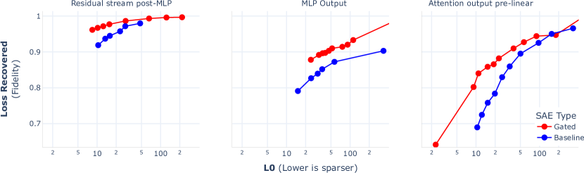
Figure 1: The performance of Gated SAEs compared to the baseline SAE at Layer 20 in Gemma-7B (log-scale axes from L0=2 to L0=200). The SAEs are trained with equal compute, since the baseline SAEs have 50% more learned features (Section 4.1). This performance improvement holds in layers throughout GELU-1L, Pythia-2.8B and Gemma-7B (Appendix B). Full detail in Table 2 and 4.

2 Sparse Autoencoder Background

In this section we summarise the concepts and notation necessary to understand existing SAE architectures and training methods, which we call the baseline SAE. We define Gated SAEs in Section 3.2. We follow notation broadly similar to Bricken et al. (2023) and recommend that work as a more complete introduction to training SAEs on LMs.

As motivated in Section 1, we wish to decompose a model’s activation $\mathbf{x}\in\mathbb{R}^{n}$ into a sparse, linear combination of feature directions:

$$\mathbf{x}\approx\mathbf{x}_{0}+\sum_{i=1}^{M}f_{i}(\mathbf{x})\mathbf{d}_{i},$$ (1)

where $\mathbf{d}_{i}$ are $M\gg n$ latent unit-norm feature directions, and the sparse coefficients $f_{i}(\mathbf{x})\geq 0$ are the corresponding feature activations for $\mathbf{x}$. The right-hand side of Eq. 1 naturally has the structure of an autoencoder: an input activation $\mathbf{x}$ is encoded into a (sparse) feature activations vector $\mathbf{f}(\mathbf{x})\in\mathbb{R}^{M}$, which in turn is linearly decoded to reconstruct $\mathbf{x}$.

2.1 Baseline Architecture

Using this correspondence, Bricken et al. (2023) and subsequent works attempt to learn a suitable sparse decomposition by parameterising a single-layer autoencoder $\left(\mathbf{f},\hat{\mathbf{x}}\right)$ defined by:

$${\mathbf{f}}(\mathbf{x}) :=\text{ReLU}\left(\mathbf{W}_{\text{enc}}\left(\mathbf{x}-\mathbf{b}_{\text{dec}}\right)+\mathbf{b}_{\text{enc}}\right)$$ (2)

$$\hat{\mathbf{x}}({\mathbf{f}}) :=\mathbf{W}_{\text{dec}}{\mathbf{f}}+\mathbf{b}_{\text{dec}}$$ (3)

and training it (Section 2.2) to reconstruct a large dataset of model activations $\mathbf{x}\sim\mathcal{D}$, constraining the hidden representation $\mathbf{f}$ to be sparse. Once the sparse autoencoder has been trained, we obtain a decomposition of the form of Eq. 1 by identifying the (suitably normalised) columns of the decoder weight matrix $\mathbf{W}_{\text{dec}}\in\mathbb{R}^{M\times n}$ with the dictionary of feature directions $\mathbf{d_{i}}$, the decoder bias $\mathbf{b}_{\text{dec}}\in\mathbb{R}^{n}$ with the centering term $\mathbf{x}_{0}$, and the (suitably normalised) entries of the latent representation $\mathbf{f}(\mathbf{x})\in\mathbb{R}^{M}$ with the feature activations $f_{i}(\mathbf{x})$.

2.2 Baseline Training Methodology

To train sparse autoencoders, Bricken et al. (2023) use a loss function that jointly encourages (i) faithful reconstruction and (ii) sparsity. Reconstruction fidelity is encouraged by the squared distance between SAE input and its reconstruction, $\left\lVert\mathbf{x}-\hat{\mathbf{x}}(\mathbf{f}(\mathbf{x}))\right\rVert_{2}^{2}$, which we call the reconstruction loss, whereas sparsity is encouraged by the L1 norm of the active features, $\left\lVert\mathbf{f}(\mathbf{x})\right\rVert_{1}$, which we call the sparsity penalty. Balancing these two terms with a L1 coefficient $\lambda$, the loss used to optimize SAEs is given by

$$\mathcal{L}(\mathbf{x}):=\left\lVert\mathbf{x}-\hat{\mathbf{x}}(\mathbf{f}(\mathbf{x}))\right\rVert_{2}^{2}+\lambda\left\lVert\mathbf{f}(\mathbf{x})\right\rVert_{1}.$$ (4)

Since it is possible to arbitrarily reduce the sparsity loss term without affecting reconstructions or sparsity by simply scaling down encoder outputs and scaling up the norm of the decoder weights, it is important to constrain the norms of the columns of $\mathbf{W}_{\text{dec}}$ during training. Following Bricken et al. (2023), we constrain columns to have exactly unit norm. See Appendix D for full details about our (Gated and baseline) SAE training.

2.3 Evaluation

To get a sense of the quality of trained SAEs we use two metrics from Bricken et al. (2023): L0, a measure of SAE sparsity and loss recovered, a measure of SAE reconstruction fidelity.

• The L0 of a SAE is defined by the average number of active features on a given input, i.e $\mathbb{E}_{\mathbf{x}\sim\mathcal{D}}\left\lVert\mathbf{f}(\mathbf{x})\right\rVert_{0}$.

• The loss recovered of a SAE is calculated from the average cross-entropy loss of the language model on an evaluation dataset, when the SAE’s reconstructions are spliced into it. If we denote by $\text{CE}(\mathbf{\phi})$ the average loss of the language model when we splice in a function $\mathbf{\phi}:\mathbb{R}^{n}\to\mathbb{R}^{n}$ at the SAE’s site during the model’s forward pass, then loss recovered is

  $$1-\frac{\text{CE}(\mathbf{\hat{x}\circ\mathbf{f}})-\text{CE}(\mathbf{\text{Id}})}{\text{CE}(\zeta)-\text{CE}(\mathbf{\text{Id}})},$$ (5)

  Where $\mathbf{\hat{x}\circ\mathbf{f}}$ is the autoencoder function, $\zeta:\mathbf{x}\mapsto\mathbf{0}$ the zero-ablation function and $\text{Id}:\mathbf{x}\mapsto\mathbf{x}$ the identity function. According to this definition, a SAE that always outputs the zero vector as its reconstruction would get a loss recovered of 0%, whereas a SAE that reconstructs its inputs perfectly would get a loss recovered of 100%.

Of course, these metrics do not paint the full picture of SAE quality, hence we perform manual analysis of SAE interpretability in Section 4.3.

3 Gated SAEs

3.1 Motivation

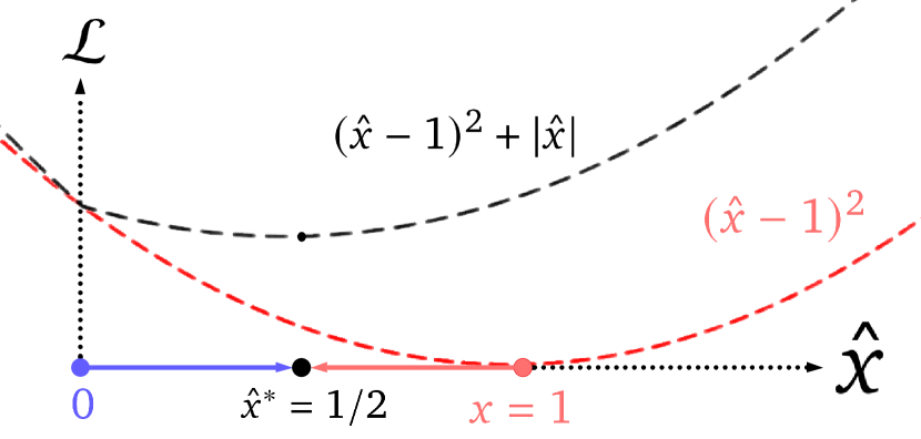
Figure 2: The L1 penalty in sparse autoencoder causes shrinkage – reconstructions are biased towards smaller norms, even when perfect reconstruction is possible.
E.g. a single-feature SAE (with L1 coefficient $\lambda=1$) reconstructs 1/2 rather than 1 when minimizing Equation 4.

The intuition behind how SAEs are trained is to maximise reconstruction fidelity at a given level of sparsity, as measured by L0, although in practice we optimize a mixture of reconstruction fidelity and L1 regularization. This difference is a source of unwanted bias in the training of a sparse autoencoder: for any fixed level of sparsity, a trained SAE can achieve lower loss (as defined in Eq. 4) by trading off a little reconstruction fidelity to perform better on the L1 sparsity penalty.

The clearest consequence of this bias is shrinkage (Wright and Sharkey, 2024), illustrated in Figure 2. Holding the decoder $\hat{\mathbf{x}}(\bullet)$ fixed, the L1 penalty pushes feature activations $\mathbf{f}(\mathbf{x})$ towards zero, while the reconstruction loss pushes $\mathbf{f}(\mathbf{x})$ high enough to produce an accurate reconstruction. Thus, the optimal value is somewhere in between, which means it systematically underestimates the magnitude of feature activations, without any necessarily having any compensatory benefit for sparsity.

How can we reduce the bias introduced by the L1 penalty? The output of the encoder $\mathbf{f}(\mathbf{x})$ of a baseline SAE (Section 2.1) has two roles:

1. It detects which features are active (according to whether the outputs are zero or strictly positive). For this role, the L1 penalty is necessary to ensure the decomposition is sparse.

2. It estimates the magnitudes of active features. For this role, the L1 penalty is a source of unwanted bias.

If we could separate out these two functions of the SAE encoder, we could design a training loss that narrows down the scope of SAE parameters that are affected (and therefore to some extent biased) by the L1 sparsity penalty to precisely those parameters that are involved in feature detection, minimising its impact on parameters used in feature magnitude estimation.

3.2 Gated SAEs

3.2.1 Architecture

How should we modify the baseline SAE encoder to achieve this separation of concerns? Our solution is to replace the single-layer ReLU encoder of a baseline SAE with a gated ReLU encoder. Taking inspiration from Gated Linear Units (Shazeer, 2020; Dauphin et al., 2017), we define the gated encoder as follows:

$$\tilde{\mathbf{f}}(\mathbf{x}):=\underbrace{\mathbb{1}[\overbrace{(\mathbf{W}_{\text{gate}}(\mathbf{x}-\mathbf{b}_{\text{dec}})+\mathbf{b}_{\text{gate}})}^{\boldsymbol{\pi}_{\text{gate}}(\mathbf{x})}>\mathbf{0}]}_{\mathbf{f}_{\text{gate}}(\mathbf{x})}\odot\underbrace{\text{ReLU}(\mathbf{W}_{\text{mag}}(\mathbf{x}-\mathbf{b}_{\text{dec}})+\mathbf{b}_{\text{mag}})}_{\mathbf{f}_{\text{mag}}(\mathbf{x})},$$ (6)

where $\mathbb{1}[\bullet>\mathbf{0}]$ is the (pointwise) Heaviside step function and $\odot$ denotes elementwise multiplication. Here, $\mathbf{f}_{\text{gate}}$ determines which features are deemed to be active, while $\mathbf{f}_{\text{mag}}$ estimates feature activation magnitudes (which only matter for features that have been deemed to be active); $\boldsymbol{\pi}_{\text{gate}}(\mathbf{x})$ are the $\mathbf{f}_{\text{gate}}$ sub-layer’s pre-activations, which are used in the gated SAE loss, defined below.

Naively, we appear to have doubled the number of parameters in the encoder, increasing the total number of parameters by 50%. We mitigate this through weight sharing: we parameterise these layers so that the two layers share the same projection directions, but allow the norms of these directions as well as the layer biases to differ. Concretely, we define $\mathbf{W}_{\text{mag}}$ in terms of $\mathbf{W}_{\text{gate}}$ and an additional vector-valued rescaling parameter $\mathbf{r}_{\text{mag}}\in\mathbb{R}^{M}$ as follows:

$$\left(\mathbf{W}_{\text{mag}}\right)_{ij}:=\left(\exp(\mathbf{r}_{\text{mag}})\right)_{i}\cdot\left(\mathbf{W}_{\text{gate}}\right)_{ij}.$$ (7)

See Fig. 3 for an illustration of the tied-weight Gated SAEs architecture. With this weight tying scheme, the Gated SAE has only $2\times M$ more parameters than a baseline SAE. In Section 5.1, we perform an ablation study showing that this weight tying scheme leads to a small increase in performance.

With tied weights, the gated encoder can be reinterpreted as a single-layer linear encoder with a non-standard and discontinuous “Jump ReLU” activation function (Erichson et al., 2019), $\sigma_{\theta}(z)$, illustrated in Fig. 4. To be precise, using the weight tying scheme of Eq. 7, $\tilde{\mathbf{f}}(\mathbf{x})$ can be re-expressed as $\tilde{\mathbf{f}}(\mathbf{x})=\sigma_{\boldsymbol{\theta}}(\mathbf{W}_{\text{mag}}\cdot\mathbf{x}+\mathbf{b}_{\text{mag}})$, with the Jump ReLU gap given by $\boldsymbol{\theta}=\mathbf{b}_{\text{mag}}-e^{\mathbf{r}_{\text{mag}}}\odot\mathbf{b}_{\text{gate}}$; see Appendix E for an explanation. We think this is a useful intuition for reasoning about how Gated SAEs reconstruct activations in practice. See Appendix F for a walkthrough of a toy example where an SAE with Jump ReLUs outperforms one with standard ReLUs.

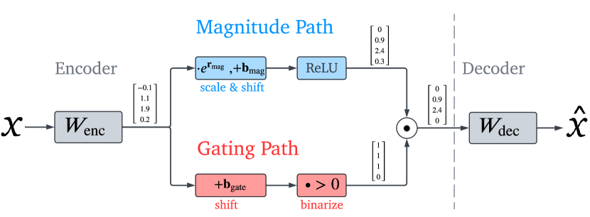
Figure 3: The Gated SAE architecture with weight sharing between the gating and magnitude paths, shown with an example input.

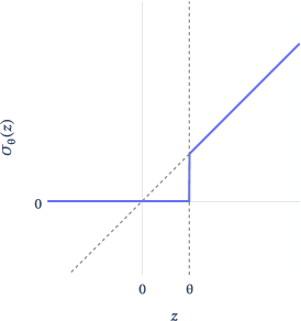
Figure 4: After applying the weight sharing scheme of Eq. 7, a gated encoder becomes equivalent to a single layer linear encoder with a Jump ReLU (Erichson et al., 2019) activation function $\sigma_{\theta}$, illustrated above.

3.2.2 Training Gated SAEs

A natural idea for training gated SAEs would be to apply Eq. 4, while restricting the sparsity penalty to just $\mathbf{f}_{\text{gate}}$:

$$\mathcal{L}_{\text{incorrect}}(\mathbf{x}):=\underbrace{\left\lVert\mathbf{x}-\hat{\mathbf{x}}\left(\tilde{\mathbf{f}}(\mathbf{x})\right)\right\rVert_{2}^{2}}_{\mathcal{L}_{\text{reconstruct}}}+\underbrace{\lambda\left\lVert\mathbf{f}_{\text{gate}}(\mathbf{x})\right\rVert_{1}}_{\mathcal{L}_{\text{sparsity}}}$$

Unfortunately, due to the Heaviside step activation function in $\mathbf{f}_{\text{gate}}$, no gradients would propagate to $\mathbf{W}_{\text{gate}}$ and $\mathbf{b}_{\text{gate}}$. To mitigate this for the sparsity penalty, we instead apply the L1 norm to the positive parts of the preactivation, $\text{ReLU}\left(\boldsymbol{\pi}_{\text{gate}}(\mathbf{x})\right)$. To ensure $\mathbf{f}_{\text{gate}}$ aids reconstruction by detecting active features, we add an auxiliary task requiring that these same rectified preactivations can be used by the decoder to produce a good reconstruction:

$$\mathcal{L}_{\text{gated}}(\mathbf{x}):=\underbrace{\left\lVert\mathbf{x}-\hat{\mathbf{x}}\left(\tilde{\mathbf{f}}(\mathbf{x})\right)\right\rVert_{2}^{2}}_{\mathcal{L}_{\text{reconstruct}}}+\underbrace{\lambda\left\lVert\text{ReLU}(\boldsymbol{\pi}_{\text{gate}}(\mathbf{x}))\right\rVert_{1}}_{\mathcal{L}_{\text{sparsity}}}+\underbrace{\left\lVert\mathbf{x}-\hat{\mathbf{x}}_{\text{frozen}}\left(\text{ReLU}\left(\boldsymbol{\pi}_{\text{gate}}(\mathbf{x})\right)\right)\right\rVert_{2}^{2}}_{\mathcal{L}_{\text{aux}}}$$ (8)

where $\hat{\mathbf{x}}_{\text{frozen}}$ is a frozen copy of the decoder, $\hat{\mathbf{x}}_{\text{frozen}}(\mathbf{f}):=\mathbf{W}_{\text{dec}}^{\text{copy}}\mathbf{f}+\mathbf{b}_{\text{dec}}^{\text{copy}}$, to ensure that gradients from $\mathcal{L}_{\text{aux}}$ do not propagate back to $\mathbf{W}_{\text{dec}}$ or $\mathbf{b}_{\text{dec}}$. This can typically be implemented by stop gradient operations rather than creating copies – see Appendix G for pseudo-code for the forward pass and loss function.

To calculate this loss (or its gradient), we have to run the decoder twice: once to perform the main reconstruction for $\mathcal{L}_{\text{reconstruct}}$ and once to perform the auxiliary reconstruction for $\mathcal{L}_{\text{aux}}$. This leads to a 50% increase in the compute required to perform a training update step. However, the increase in overall training time is typically much less, as in our experience much of the training wall clock time goes to generating language model activations (if these are being generated on the fly) or disk I/O (if training on saved activations).

4 Evaluation

In this section we benchmark Gated SAEs across a large variety of models and at different sites (Section 4.1), show that they resolve the shrinkage problem (Section 4.2), and show that they produce features that are similarly interpretable to baseline SAE features according to expert human raters, although we could not conclusively determine whether one is better than the other (Section 4.3).

4.1 Comprehensive Benchmarking

In this subsection we show that Gated SAEs are a Pareto improvement over baseline SAEs on the loss recovered and L0 metrics (Section 2.3). We show this by evaluating SAEs trained to reconstruct:

1. The MLP neuron activations in GELU-1L, which is the closest direct comparison to Bricken et al. (2023);

2. The MLP outputs, attention layer outputs (taken pre $W_{O}$ as in Kissane et al. (2024a)) and residual stream activations in 5 different layers throughout Pythia-2.8B and four different layers in the Gemma-7B base model.

In both experiments, we vary the L1 coefficient $\lambda$ (Section 2.2) used to train the SAEs, which enables us to compare the Pareto frontiers of L0 and loss recovered between Gated and baseline SAEs.

Gated SAEs require at most 1.5$\times$ more compute to train than regular SAEs (Section 3.2.2). To therefore ensure fair comparison in our evaluations, we compare Gated SAEs to baseline SAEs with 50% more learned features. We show the results for GELU-1L in Figure 5 and the results for Pythia-2.8B and Gemma-7B in Appendix B. In Appendix B (Figure 12), at all sites tested, Gated SAEs are a Pareto improvement over regular SAEs. In some cases in Figure 12 and 13 there is a non-monotonic Pareto frontier. We attribute this to difficulties training SAEs (Section D.1.3).

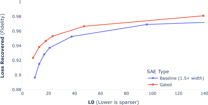
Figure 5: Gated SAEs offer better reconstruction fidelity (as measured by loss recovered) at any given level of feature sparsity (as measured by L0). This plot compares Gated and baseline SAEs trained on GELU-1L neuron activations; see Appendix B for comparisons on Pythia-2.8B and Gemma-7B.

4.2 Shrinkage

As described in Section 3.1, the L1 sparsity penalty used to train baseline SAEs causes feature activations to be systematically underestimated, a phenomenon called shrinkage. Since this in turn shrinks the reconstructions produced by the SAE decoder, we can observe the extent to which a trained SAE is affected by shrinkage by measuring the average norm of its reconstructions.

Concretely, the metric we use is the relative reconstruction bias,

$$\gamma:=\operatorname*{arg\,min}_{\gamma^{\prime}}\mathbb{E}_{\mathbf{x}\sim\mathcal{D}}\left[\left\lVert\hat{\mathbf{x}}_{\text{SAE}}(\mathbf{x})/\gamma^{\prime}-\mathbf{x}\right\rVert_{2}^{2}\right],$$ (9)

i.e. $\gamma^{-1}$ is the optimum multiplicative factor by which an SAE’s reconstructions should be rescaled in order to minimise the L2 reconstruction loss; $\gamma=1$ for an unbiased SAE and $\gamma<1$ when there’s shrinkage. Explicitly solving the optimization problem in Eq. 9, the relative reconstruction bias can be expressed analytically in terms of the mean SAE reconstruction loss, the mean squared norm of input activations and the mean squared norm of SAE reconstructions, making $\gamma$ easy to compute and track during training:

$$\gamma=\frac{\mathbb{E}_{\mathbf{x}\sim\mathcal{D}}\left[\left\lVert\hat{\mathbf{x}}_{\text{SAE}}\left(\mathbf{x}\right)\right\rVert_{2}^{2}\right]}{\mathbb{E}_{\mathbf{x}\sim\mathcal{D}}\Big{[}\hat{\mathbf{x}}_{\text{SAE}}\left(\mathbf{x}\right)\cdot\mathbf{x}\Big{]}}=\frac{2\,\mathbb{E}_{\mathbf{x}\sim\mathcal{D}}\left[\left\lVert\hat{\mathbf{x}}_{\text{SAE}}\left(\mathbf{x}\right)\right\rVert_{2}^{2}\right]}{\mathbb{E}_{\mathbf{x}\sim\mathcal{D}}\left[\left\lVert\hat{\mathbf{x}}_{\text{SAE}}\left(\mathbf{x}\right)\right\rVert_{2}^{2}\right]+\mathbb{E}_{\mathbf{x}\sim\mathcal{D}}\left[\left\lVert\mathbf{x}\right\rVert_{2}^{2}\right]-\mathbb{E}_{\mathbf{x}\sim\mathcal{D}}\left[\left\lVert\hat{\mathbf{x}}_{\text{SAE}}\left(\mathbf{x}\right)-\mathbf{x}\right\rVert_{2}^{2}\right]}.$$ (10)

As shown in Figure 6, Gated SAEs’ reconstructions are unbiased, with $\gamma\approx 1$, whereas baseline SAEs exhibit shrinkage ($\gamma<1$), with the impact of shrinkage getting worse as the L1 coefficient $\lambda$ increases (and L0 consequently decreases). In Appendix C we show that this result generalizes to Pythia-2.8B.

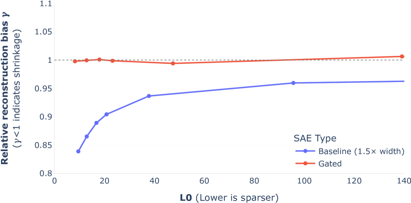
Figure 6: Gated SAEs address the shrinkage (GELU-1L neuron activations).

4.3 Manual Interpretability Scores

4.3.1 Experimental Methodology

While we believe that the metrics we have investigated above convey meaningful information about an SAE’s quality, they are only imperfect proxies. As of now, there is no consensus on how to gauge the degree to which a learned feature is ‘interpretable’. To gain a more qualitative understanding of the difference between the learned dictionary feature, we conduct a blinded human rater experiment, in which we rated the interpretability of a set of randomly sampled features.

We study a variety of SAEs from different layers and sites.

For Pythia-2.8B we had 5 raters, who each rated one feature from baseline and Gated SAEs trained on each (Site, Layer) pair from Figure 12, for a total of 150 features. For Gemma-7B we had 7 raters; one rated 2 features each, and the rest 1 feature each, from baseline or Gated SAEs trained on each (Site, Layer) pair from Figure 13, for a total of 192 features.

In both cases, the raters were shown the features in random order, without revealing what SAE, site, or layer they came from. To assess a feature, the rater needed to decide whether there is an explanation of the feature’s behavior, in particular for its highest activating examples. The rater then entered that explanation (if applicable) and selected whether the feature is interpretable (‘Yes’), uninterpretable (‘No’) or maybe interpretable (‘Maybe’). As an interface we use an open source SAE visualizer library (McDougall, 2024).

4.3.2 Statistical Analysis

To test whether Gated SAEs may be more interpretable and estimate the difference, we pair our datapoints according to all covariates (model, layer, site, rater); this lets us control for all of them without making any parametric assumptions, and thus reduces variance in the comparison. We use a one-sided paired Wilcoxon-Pratt signed-rank test, and provide a 90% BCa bootstrap confidence interval for the mean difference between Baseline and Gated labels, where we count ‘No’ as 0, ‘Maybe’ as 1, and ‘Yes’ as 2. Overall the test of the null hypothesis that Gated SAEs are at most as interpretable as Baseline SAEs gets $p=.060$ (estimate .13, mean difference CI $[0,.26]$). This breaks down into $p=.15$ on just the Pythia-2.8B data (mean difference CI $[-.07,.33]$), and $p=.13$ on just the Gemma-7B data (mean difference CI $[-.04,.29]$).

A Mann-Whitney U rank test on the label differences, comparing results on the two models, fails to reject ($p=.95$) the null hypothesis that they’re from the same distribution; the same test directly on the labels similarly fails to reject ($p=.84$) the null hypothesis that they’re similarly interpretable overall.

The contingency tables used for these results are shown in Figure 7. The overall conclusion is that, while we can’t definitively say the Gated SAE features are more interpretable than those from the Baseline SAEs, they are at least comparable. We provide more analysis of how these break down by site and layer in Appendix H.

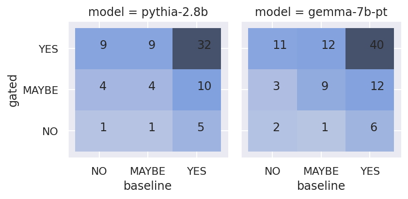
Figure 7: Contingency table showing Gated vs Baseline interpretability labels from our paired study results, for Pythia-2.8B and Gemma-7B.

5 Why do Gated SAEs improve SAE training?

In this section we describe an ablation study that reveals the important parts of Gated SAE training (Section 5.1) and benchmark Gated SAEs against a closely related approach to resolving shrinkage (Section 5.2).

5.1 Ablation Study

In this section, we vary several parts of the Gated SAE training methodology (Section 3.2) to gain insight into which aspects of the training are required for the observed improvement in performance. Gated SAEs differ from baseline SAEs in many respect, making it easy to incorrectly attribute the performance gains to spurious details without a careful ablation study. Figure 8 shows Pareto frontiers for these variations and below which we describe each variation in turn and discuss our interpretation of the results.

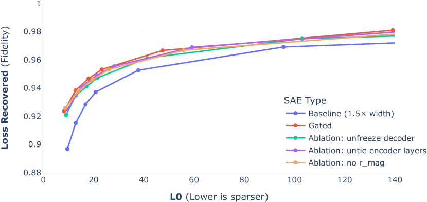
Figure 8: Our ablation study on GELU-1L MLP neuron activations indicates: (a) the importance of freezing the decoder in the auxiliary task $\mathcal{L}_{\text{aux}}$ used to train $\mathbf{f}_{\text{gate}}$’s parameters; (b) tying encoder weights according to Eq. 7 is slightly beneficial for performance (in addition to yielding a significant reduction in parameter count and inference compute); (c) further simplifying the encoder weight tying scheme in Eq. 7 by removing $\mathbf{r}_{\text{mag}}$ is mildly harmful to performance.

1. Unfreeze decoder: Here we unfreeze the decoder weights in $\mathcal{L}_{\text{aux}}$ – i.e. allow this auxiliary task to update the decoder weights in addition to training $\mathbf{f}_{\text{gate}}$’s parameters. Although this (slightly) simplifies the loss, there is a reduction in performance, providing evidence in support of the hypothesis that it is beneficial to limit the impact of the L1 sparsity penalty to just those parameters in the SAE that need it – i.e. those used to detect which features are active.

2. No $\mathbf{r}_{\text{mag}}$: Here we remove the $\mathbf{r}_{\text{mag}}$ scaling parameter in Eq. 7, effectively setting it to zero (so that we multiply by $e^{0}=1$); this further ties $\mathbf{f}_{\text{gate}}$’s and $\mathbf{f}_{\text{mag}}$’s parameters together. With this change, the two encoder sublayers’ preactivations can at most differ by an elementwise shift. There is a slight drop in performance, suggesting $\mathbf{r}_{\text{mag}}$ contributes somewhat (but not critically) to the improved performance of the Gated SAE.

3. Untied encoders: Here we check whether our choice to share the majority of parameters between the two encoders has meaningfully hurt performance, by training Gated SAEs with gating and ReLU encoder parameters completely untied. Despite the greater expressive power of an untied encoder, we see no improvement in performance – in fact a slight deterioration. This suggests our tying scheme (Eq. 7) – where encoder directions are shared, but magnitudes and biases aren’t – is effective at capturing the advantages of using a gated SAE while avoiding the 50% increase in parameter count and inference-time compute of using an untied SAE.

5.2 Is it sufficient to just address shrinkage?

As explained in Section 3.1, SAEs trained with the baseline architecture and L1 loss systematically underestimate the magnitudes of latent features’ activations (i.e. shrinkage). Gated SAEs, through modifications to their architecture and loss function, overcome these limitations, thereby addressing shrinkage.

It is natural to ask to what extent the performance improvement of Gated SAEs is solely attributable to addressing shrinkage. Although addressing shrinkage would – all else staying equal – improve reconstruction fidelity, it is not the only way to improve SAEs’ performance: for example, gated SAEs could also improve upon baseline SAEs by learning better encoder directions (for estimating when features are active and their magnitudes) or by learning better decoder directions (i.e. better dictionaries for reconstructing activations).

In this section, we try to answer this question by comparing Gated SAEs trained as described in Section 3.2.2 with an alternative (architecturally equivalent) approach that also addresses shrinkage, but in a way that uses frozen encoder and decoder directions from a baseline SAE of equal dictionary size. Any performance improvement over baseline SAEs obtained by this alternative approach (which we dub “baseline + rescale & shift”) can only be due to better estimations of active feature magnitudes, since by construction an SAE parameterised by “baseline + rescale & shift” shares the same encoder and decoder directions as a baseline SAE.

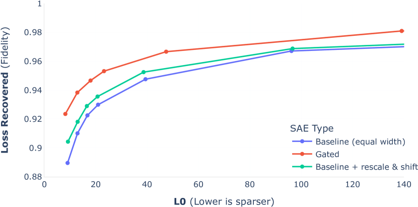
Figure 9: Evidence from GELU-1L that the performance improvement of gated SAEs does not solely arise from addressing shrinkage (systematic underestimation of latent feature activations). Taking a frozen baseline SAE’s parameters and learning $\mathbf{r}_{\text{mag}}$ and $\mathbf{b}_{\text{mag}}$ parameters on top of them (green line) does successfully resolve shrinkage, by decoupling feature magnitude estimation from active feature detection. However, it explains only a small part of the performance increase of gated SAEs (red line) over baseline SAEs (blue line).

As shown in Fig. 9, although resolving shrinkage only (“baseline + rescale & shift”) does improvement baseline SAEs’ performance a little, a significant gap remains with respect to the performance of gated SAEs. This suggests that the benefit of the gated architecture and loss comes from learning better encoder and decoder directions, not just from overcoming shrinkage. In Appendix A we explore further how Gated and baseline SAEs’ decoders differ by replacing their respective encoders with an optimization algorithm at inference time.

6 Related Work

Mechanistic Interpretability. We hope that our improvements to Sparse Autoencoders are helpful for mechanistic interpretability research. Recent mechanistic interpretability work has found recurring components in small and large LMs (Olsson et al., 2022), identified computational subgraphs that carry out specific tasks in small LMs (circuits; Wang et al. (2023)) and reverse-engineered how toy tasks are carried out in small transformers (Nanda et al., 2023). Limitations of existing work include (i) how they only study narrow subsets of the natural language training distribution are studied (though see McDougall et al. (2023)) and (ii) current work has not explained how frontier language models function mechanistically (OpenAI, 2023; Gemini Team, 2024; Anthropic AI, 2024). SAEs may be key to explaining model behaviour across the whole training distribution (Bricken et al., 2023) and are trained without supervision, which may enable future work to explain how larger models function on broader tasks.

Classical Dictionary Learning. Our work builds on a large amount of research that precedes transformers, and even deep learning. For example, sparse coding (Elad, 2010) studies how discrete and continuous representations can involve more representations than basis vectors, like our setup in Section 1, and sparse representations are also studied in neuroscience (Thorpe, 1989; Olshausen and Field, 1997). Further, shrinkage (Section 4.2) is built into the Lasso (Tibshirani, 1996) and well-studied in statistical learning (Hastie et al., 2015). One dictionary learning algorithm, k-SVD (Aharon et al., 2006) also uses two stages to learn a dictionary like Gated SAEs.

Dictionary Learning in Language Models. Early work into applying Dictionary Learning to LMs include Sharkey et al. (2022) (on a GPT-2-like model), Yun et al. (2023) (on a BERT model), Tamkin et al. (2023) (with discrete features, and during LM pretraining) and Cunningham et al. (2023) (on a small Pythia model). Bricken et al. (2023)’s work later provided a widely-scoped analysis of SAEs trained on a 1L model, evaluating the loss when splicing the SAE into the forward pass (Section 4.1), evaluating the impact of learned features on LM rollouts, and visualizing and interpreting all learned features with autointerpretability (Bills et al., 2023). Following this work, other researchers have extended SAE training to attention layer outputs (Kissane et al., 2024a, b) and residual stream states (Bloom, 2024).

Dictionary Learning’s Limitations and Improvements. Wright and Sharkey (2024) raised awareness of shrinkage (Section 4.2) and proposed addressing this via decoder finetuning. A difficulty with this approach is that it is not possible to fine tune all the SAEs parameters in this way without losing sparsity and/or interpretability of feature directions. This limits the extent to which fine-tuning can remove the biases baked into the SAEs parameters during L1-based pre-training. Gated SAEs address this issue (Section 3.2). Marks et al. (2024) stress-test how useful SAEs are, and find success but also rely on methods that leave many error nodes in their computational subgraphs, which represent the difference between SAE reconstructions and the ground truth. A series of updates to the work in Bricken et al. (2023) have also proposed SAE training methodology improvements (Olah et al., 2024; Templeton et al., 2024; Batson et al., 2024). In parallel to our work, Taggart (2024) finds early improvements with a similar Jump ReLU (Erichson et al., 2019) architecture change to SAEs, but with a different loss function, and without addressing the problems of L1.

Disentanglement (Bengio, 2013) aims to learn representations that separate out distinct, independent ‘factors of variation’ of the underlying data generating process. This is somewhat similar to our aims with dictionary learning, as we want to separate an activation vector into distinct, sparse factors of variation (weights on feature directions), although the dictionary elements are not completely independent, as it may not be possible to accurately represent two features simultaneously due to interference between non-orthogonal dictionary features. Methods explicitly motivated by learning a disentangled representation typically enforce a prior structure on the learned representation, typically that features are aligned with the basis of a latent space (Kim and Mnih, 2018; Mathieu et al., 2019; Chen et al., 2016, 2018). In contrast, in our work we focus on the representation space of a pre-trained language model, rather than trying to learn a representation directly from data, and enforce a different prior structure, of decomposition into a sparse linear combination of an overcomplete basis. In a sense, our work proceeds from the theory that language models have succeeded in learning a disentangled representation of the data with a particular structure, which we are trying to recover.

7 Conclusion

In this work we introduced Gated SAEs (Section 3.2) which are a Pareto improvement in terms of reconstruction quality and sparisty compared to baseline SAEs (Section 4.1), and are comparably interpretable (Section 4.3). We showed via an ablation study that every key part of the Gated SAE methodology was necessary for strong performance (Section 5.1). This represents significant progress on improving Dictionary Learning in LLMs – at many sites, Gated SAEs require half the L0 to achieve the same loss recovered (Figure 12). This is likely to improve work that uses SAEs to steer language models (Nanda et al., 2024), interpret circuits (Marks et al., 2024), or understand language model components across the full distribution (Bricken et al., 2023).

Limitations. Our work, like all sparse autoencoder research, is motivated by several assumptions about the sparsity and linearity of computation in Large Language Models (Section 1). If these assumptions are false, our work may still be useful (see footnote 1), but we may be making incorrect conclusions from work using SAEs, since they bake in the sparsity and linearity assumptions. Separately, our work complicates SAE training with a more complex encoder.

One worry about increasing the expressivity of sparse autoencoders is that they will overfit when reconstructing activations (Olah et al., 2023, Dictionary Learning Worries), since the underlying model only uses simple MLPs and attention heads, and in particular lacks discontinuities such as step functions. Overall we do not see evidence for this. Our evaluations use held-out test data and we check for interpretability manually. But these evaluations are not totally comprehensive: for example, they do not test that the dictionaries learned contain causally meaningful intermediate variables in the model’s computation. The discontinuity in particular introduces issues with methods like integrated gradients (Sundararajan et al., 2017) that discretely approximate a path integral, as applied to SAEs by Marks et al. (2024).

Finally, it could be argued that some of the performance gap between Gated and baseline SAEs could be closed by inexpensive inference-time interventions that prune the many low activating features that tend to appear in baseline SAEs – because baseline SAEs don’t have a thresholding mechanism like Gated SAEs do (Appendix E). Without such interventions, these low activating features increase baseline SAEs’ L0 at a given loss recovered without contributing much to reconstruction (due to low magnitude), and with unclear impact on interpretability.

Future work. Future work could verify that Gated SAEs continue to improve dictionary learning beyond 7B base LLMs, such as by extending to larger chat models, or even to multimodal or Mixture-of-Experts models. Alternatively, work could look into the features learned by Gated and baseline SAEs and determine whether the architectures have differences in inductive biases beyond those we noted in this work. We expect it may be possible to further improve Gated SAEs’ performance through additional tweaks to the architecture and training procedure. Finally, we would be most excited to work on using dictionary learning techniques to further interpretability in general, such as to improve circuit finding (Conmy et al., 2023; Marks et al., 2024) or steering (Turner et al., 2023) in language models, and hope that Gated SAEs can serve to accelerate such work.

8 Acknowledgements

We would like to thank Romeo Valentin for conversations that got us thinking about k-SVD in the context of SAEs, which inspired part of our work. Additionally, we are grateful for Vladimir Mikulik’s detailed feedback on a draft of this work which greatly improved our presentation, and Nicholas Sonnerat’s work on our codebase and help with feature labelling. We would also like to thank Glen Taggart who found in parallel work (Taggart, 2024) that a similar method gave improvements to SAE training, helping give us more confidence in our results. Finally, we are grateful to Sam Marks for pointing out an error in the derivation of relative reconstruction bias in an earlier version of this paper.

9 Author contributions

Senthooran Rajamanoharan developed the Gated SAE architecture and training methodology, inspired by discussions with Lewis Smith on the topic of shrinkage. Arthur Conmy and Senthooran Rajamanoharan performed the mainline experiments in Section 4 and Section 5 and led the writing of all sections of the paper. Tom Lieberum implemented the manual interpretability study of Section 4.3, which was designed and analysed by János Kramár. Tom Lieberum also created Fig. 3. Lewis Smith contributed Appendix A and Neel Nanda contributed Appendix F. Our SAE codebase was designed by Vikrant Varma who implemented it with Tom Lieberum, and was scaled to Gemma by Arthur Conmy, with contributions from Senthooran Rajamanoharan and Lewis Smith. János Kramár built most of our underlying interpretability infrastructure. Rohin Shah and Neel Nanda edited the manuscript and provided leadership and advice throughout the project.

Appendix

Appendix A Inference-time optimization

The task SAEs perform can be split into two sub-tasks: sparse coding, or learning a set of features from a dataset, and sparse approximation, where a given datapoint is approximated as a sparse linear combination of these features. The decoder weights are the set of learned features, and the mapping represented by the encoder is a sparse approximation algorithm. Formally, sparse approximation is the problem of finding a vector $\boldsymbol{\alpha}$ that minimises;

$$\boldsymbol{\alpha}=\arg\min\left\lVert\mathbf{x}-\mathbf{D}\boldsymbol{\alpha}\right\rVert^{2}_{2}\;\;s.t.\;\;\left\lVert\boldsymbol{\alpha}\right\rVert_{0}<\gamma$$ (11)

i.e. that best reconstructs the signal $\mathbf{x}$ as a linear combination of vectors in a dictionary $\mathbf{D}$, subject to a constraint on the L0 pseudo-norm on $\boldsymbol{\alpha}$. Sparse approximation is a well studied problem, and SAEs are a weak sparse approximation algorithm. SAEs, at least in the formulation conventional in dictionary learning for language models, in fact solve a slightly more restricted version of this problem where the weights $\boldsymbol{\alpha}$ on each feature are constrained to be non-negative, leading to the related problem

$$\boldsymbol{\alpha}=\arg\min\left\lVert\mathbf{x}-\mathbf{D}\boldsymbol{\alpha}\right\rVert^{2}_{2}\;\;s.t.\;\;\left\lVert\boldsymbol{\alpha}\right\rVert_{0}<\gamma,\boldsymbol{\alpha}>0$$ (12)

In this paper, we do not explore using more powerful algorithms for sparse coding. This is partly because we are using SAEs not just to recover a sparse reconstruction of activations of a LM; ideally we hope that the learned features will coincide with the linear representations actually used by the LM, under the superposition hypothesis. Prior work (Bricken et al., 2023) has argued that SAEs are more likely to recover these due to the correspondence between the SAE encoder and the structure of the network itself; the argument is that it is implausible that the network can make use of features which can only be recovered from the vector via an iterative optimisation algorithm, whereas the structure of the SAE means that it can only find features whose presence can be predicted well by a simple linear mapping. Whether this is true remains, in our view, an important question for future work, but we do not address it in this paper.

In this section we discuss some results obtained by using the dictionaries learned via SAE training, but replacing the encoder with a different sparse approximation algorithm at inference time. This allows us to compare the dictionaries learned by different SAE training regimes independently of the quality of the encoder. It also allows us to examine the gap between the sparse reconstruction performed by the encoder against the baseline of a more powerful sparse approximation algorithm. As mentioned, for a fair comparison to the task the encoder is trained for, it is important to solve the sparse approximation problem of Eq. 12, rather than the more conventional formulation of Eq. 11, but most sparse approximation algorithms can be modified to solve this with relatively minor changes.

Solving Eq. 12 exactly is equivalent to integer linear programming, and is NP hard. The integer linear programs in question would be large, as our SAE decoders routinely have hundreds of thousands of features, and solving them to guaranteed optimality would likely be intractable. Instead, as is commonly done, we use iterative greedy algorithms to find an approximate solution. While the solution found by these sparse approximation algorithms is not guaranteed to be the global optimum, these are significantly more powerful than the SAE encoder, and we feel it is acceptable in practice to treat them as an upper bound on possible encoder performance.

For all results in this section, we use gradient pursuit, as described in Blumensath and Davies (2008), as our inference time optimisation (ITO) algorithm. This algorithm is a variant of orthogonal matching pursuit (Pati et al., 1993) which solves the orgothonalisation of the residual to the span of chosen dictionary elements approximately at every step rather than exactly, but which only requires matrix multiplies rather than matrix solves and is easier to implement on accelerators as a result. It is possibly not crucial for performance that our optimisation algorithm be implementable on TPUs, but being able to avoid a host-device transfer when splicing this into the forward pass allowed us to re-use our existing evaluation pipeline with minimal changes.

When we use a sparse approximation algorithm at test time, we simply use the decoder of a trained SAE as a dictionary, ignoring the encoder. This allows us to sweep the target sparsity at test time without retraining the model, meaning that we can plot an entire Pareto frontier of loss recovered against sparsity for a single decoder, as in done in Figure 11.

Figure 10 compares the loss recovered when using ITO for a suite of SAEs decoders trained with both methods at three different test time L0 thresholds. This graph shows a somewhat surprising result; while Gated SAEs learn better decoders generally, and often achieve the best loss recovered using ITO close to their training sparsity, SAE decoders are often outperformed by decoders which achieved a higher test time L0; it’s better to do ITO with a target L0 of 10 with an decoder with an achieved L0 of around 100 during training than one which was actually trained with this level of sparsity. For instance, the left hand panel in Figure 10 shows that SAEs with a training L0 of 100 are better than those with an L0 of around 10 at almost every sparsity level in terms of ITO reconstruction. However, gated SAE dictionaries have a small but real advantage over standard SAEs in terms of loss recovered at most target sparsity levels, suggesting that part of the advantage of gated SAEs is that they learn better dictionaries as well as addressing issues with shrinkage. However, there are some subtleties here; for example, we find that baseline SAEs trained with a lower sparsity penalty (higher training L0) often outperform more sparse baseline SAEs according to this measure, and the best performing baseline SAE (L0 $\approx 99$) is comparable to the best performing Gated SAE (L0 $\approx 20$).

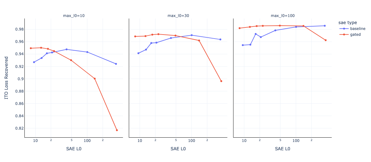
Figure 10: This figure compares the ITO performance of different decoders across a sweep for decoders trained using a baseline SAE and the gated method, at three different test time target sparsities. Gated SAEs trained at lower target sparsities consistently achieve better dictionaries by this measure. Interestingly, the best performing baseline dictionary by this measure often has a much higher test time sparsity than the target; for instance, at a test time sparsity of 30, the best baseline SAE was the one that had a test time sparsity of more like 100. This could be an artifact of the fact that the L0 measure is quite sensitive to noise, and standard SAE architectures tend to have a reasonable number of features with very low activation.

Figure 11 compares the Pareto frontiers of a baseline model and a gated model to the Pareto frontier of an ITO sweep of the best performing dictionary of each. Note that, while the Pareto curve of the baseline dictionary is formed by several models as each encoder is specialised to a given sparsity level, as mentioned, ITO lets us plot a Pareto frontier by sweeping the target sparsity with a single dictionary; here we plot only the best performing dictionary from each model type to avoid cluttering the figure. This figure suggests that the performance gap between the encoder and using ITO is smaller for the gated model. Interestingly, this cannot solely be explained by addressing shrinkage, as we demonstrate by experimenting with a baseline model which learns a rescale and shift with a frozen encoder and decoder directions.

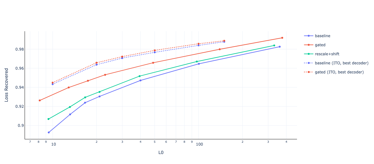
Figure 11: Pareto frontiers of a baseline SAE, a baseline SAE with learned rescale and shift (to account for shrinkage) and a gated SAE across different sparsity lambdas, compared to the ITO Pareto frontier of the best decoder of each type with ITO, varying the target sparsity. The best gated encoder is better than the best standard encoder by this measure, but the difference is marginal. As shown in the plot above, the best baseline encoder by the ITO measure had a much larger test time sparsity (around 100) than the best gated model (around 30). This figure suggests that the gap between SAE performance and ’optimal’ performance, if we assume that ITO is close to the maximum possible reconstruction using the given encoder, is much smaller for the gated model.

Appendix B More Loss Recovered / L0 Pareto frontiers

In Figure 12 we show that Gated SAEs outperform baseline SAEs. In Figure 13 we show that Gated SAEs ourperform baseline SAEs at all but one MLP output or residual stream site that we tested on.

In Figure 13 at the attention output pre-linear site at layer 27, loss recovered is bigger than 1.0. On investigation, we found that the dataset used to train the SAE was not identical to Gemma’s pretraining dataset, and at this site it was possible to mean ablate this quantity and decrease loss – explaining why SAE reconstructions had lower loss than the original model.

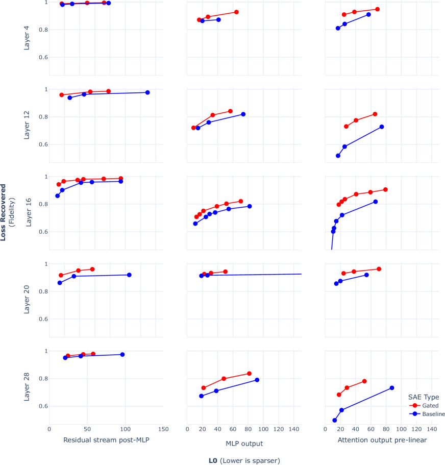
Figure 12: Gated SAEs throughout Pythia-2.8B. At all sites we tested, Gated SAEs are a Pareto improvement. In every plot, the SAE with maximal loss recovered was a Gated SAE.

Figure 13: Gated and Normal Pareto-Optimal SAEs for Gemma-7B – see Appendix B for a discussion of the anomalies (such as the Layer 27 attention output SAEs), and Table 1-4 for full stats (including points not on the Pareto frontier).

Appendix C Further Shrinkage Plots

In Figure 14, we show that Gated SAEs resolve shrinkage (as measured by relative reconstruction bias (Section 4.2)) in Pythia-2.8B.

Figure 14: Gated SAEs address the shrinkage problem (Section 4.2) in Pythia-2.8B.

Appendix D Training and evaluation: hyperparameters and other details.

D.1 Training

D.1.1 General training details

Other details of SAE training are:

• SAE Widths. Our SAEs have width $2^{17}$ for most baseline SAEs, $3\times 2^{16}$ for Gated SAEs, except for the (Pythia-2.8B, Residual Stream) sites we used $2^{15}$ for baseline and $3\times 2^{14}$ for Gated since early runs at these sites had lots of learned feature death.

• Training data. We use activations from hundreds of millions to billions of activations from LM forward passes as input data to the SAE. Following Nanda (2023), we use a shuffled buffer of these activations, so that optimization steps don’t use data from highly correlated activations.

• Resampling. We used resampling, a technique which at a high-level reinitializes features that activate extremely rarely on SAE inputs periodically throughout training. We mostly follow the approach described in the ‘Neuron Resampling’ appendix of Bricken et al. (2023), except we reapply learning rate warm-up after each resampling event, reducing learning rate to 0.1x the ordinary value, and, increasing it with a cosine schedule back to the ordinary value over the next 1000 training steps.

• Optimizer hyperparameters. We use the Adam optimizer with $\beta_{2}=0.999$ and $\beta_{1}=0.0$, following Templeton et al. (2024), as we also find this to be a slight improvement to training. We use a learning rate warm-up. See Section D.1.2 for learning rates of different experiment.

• Decoder weight norm constraints. Templeton et al. (2024) suggest constraining columns to have at most unit norm (instead of exactly unit norm), which can help distinguish between productive and unproductive feature directions (although it should have no systematic impact on performance). However, we follow the original approach of constraining columns to have exact unit norms in this work for the sake of simplicity.

• Interpreting the L1 $\lambda$ coefficients.. In our infrastructure we calculate L2 loss and then divide by $n$. In the baseline experiments we further divide the reconstruction L2 loss by $\mathbb{E}||x||_{2}$.

D.1.2 Experiment-specific training details

• We use learning rate 0.0003 for all Gated SAE experiments, and the GELU-1L baseline experiment. We swept for optimal baseline learning rates for the GELU-1L baseline to generate this value. For the Pythia-2.8B and Gemma-7B baseline SAE experiments, we divided the L2 loss by $\mathbb{E}||x||_{2}$, motivated by better hyperparameter transfer, and so changed learning rate to 0.001 and 0.00075 (full learning rate detail in tables Table 1-8). We didn’t see noticeable difference in the Pareto frontier and so did not sweep this hyperparameter further.

• We generate activations from sequences of length 128 for GELU-1L, 2048 for Pythia-2.8B and 1024 for Gemma-7B.

• We use a batch size of 4096 for all runs. We use 300,000 training steps for GELU-1L and Gemma-7B runs, and 400,000 steps for Pythia-2.8B runs.

D.1.3 Lessons learned scaling SAEs

• Learned feature death is unpredictable. In Table 1 (and other tables) there are few patterns that can be gleaned from staring at which runs have high numbers of dead learned features (called dead neurons in Bricken et al. (2023)).

• Resampling makes hyperparameter sweeps difficult. We found that resampling caused L0 and loss recovered to increase, similar to Conmy (2023).

• Training appears to converge earlier than expected. We found that we did not need 20B tokens as in Bricken et al. (2023), as generally resampling had stopped causing gains and loss curves plateaued after just over one billion tokens.

D.2 Evaluation

We evaluated the models on over a million held-out tokens. Tables 1-8 show summary stats from training runs on the Pareto frontier.

Site	Layer	Sparsity $\lambda$	LR	L0	% CE Recovered	Clean CE Loss	SAE CE Loss	0 Abl. CE Loss	Width	% Alive Features	Shrinkage $\gamma$
Resid	6	3e-05	0.001	18.1	95.28%	2.5426	3.1847	16.1549	196608	16.8%	0.982
Resid	6	2e-05	0.001	10.5	85.3%	2.5426	4.5433	16.1549	196608	5.72%	1.136
Resid	6	1e-05	0.001	19.0	91.24%	2.5426	3.7349	16.1549	196608	5.11%	1.606
Resid	6	2e-05	0.00075	29.8	96.65%	2.5426	2.9989	16.1549	196608	13.67%	1.261
Resid	6	3e-05	0.00075	25.4	97.9%	2.5426	2.8279	16.1549	196608	38.86%	0.976
Resid	6	8e-06	0.00075	29.8	91.28%	2.5426	3.7301	16.1549	196608	9.88%	1.105
Resid	6	1e-05	0.00075	57.3	97.36%	2.5426	2.9023	16.1549	196608	11.78%	1.03
Resid	6	4e-06	0.00075	69.2	95.98%	2.5426	3.0892	16.1549	196608	13.54%	1.239
Resid	6	6e-06	0.00075	40.0	95.49%	2.5426	3.1562	16.1549	196608	24.34%	1.159
Resid	13	9e-05	0.00075	14.3	96.77%	2.5426	3.4423	30.3588	196608	98.38%	0.806
Resid	13	8e-05	0.00075	17.5	97.66%	2.5426	3.1947	30.3588	196608	98.7%	0.824
Resid	13	8e-05	0.001	18.0	97.63%	2.5426	3.2021	30.3588	196608	95.35%	0.838
Resid	13	5e-05	0.00075	22.2	97.69%	2.5426	3.1849	30.3588	196608	25.78%	0.889
Resid	13	3e-05	0.00075	29.0	97.64%	2.5426	3.1986	30.3588	196608	8.55%	0.903
Resid	13	5e-05	0.001	29.5	98.71%	2.5426	2.9005	30.3588	196608	65.17%	0.867
Resid	13	3e-05	0.001	39.2	98.26%	2.5426	3.026	30.3588	196608	26.33%	0.936
Resid	13	2e-05	0.00075	56.6	98.49%	2.5426	2.9615	30.3588	196608	16.19%	0.976
Resid	13	1e-05	0.00075	101.3	97.83%	2.5426	3.1459	30.3588	196608	4.55%	1.018
Resid	20	0.00012	0.00075	10.4	91.87%	2.5426	3.9277	19.5891	196608	92.51%	0.773
Resid	20	0.0001	0.00075	13.8	93.68%	2.5426	3.6204	19.5891	196608	97.46%	0.797
Resid	20	9e-05	0.00075	16.0	94.48%	2.5426	3.4835	19.5891	196608	99.2%	0.81
Resid	20	3e-05	0.001	25.2	90.71%	2.5426	4.1258	19.5891	196608	3.11%	0.951
Resid	20	7e-05	0.001	21.3	95.73%	2.5426	3.27	19.5891	196608	99.62%	0.824
Resid	20	5e-05	0.001	27.8	97.15%	2.5426	3.0281	19.5891	196608	88.4%	0.879
Resid	20	3e-05	0.00075	39.1	96.43%	2.5426	3.1518	19.5891	196608	35.64%	1.019
Resid	20	4e-05	0.00075	46.4	97.95%	2.5426	2.8922	19.5891	196608	99.9%	0.874
Resid	20	2e-05	0.00075	49.4	95.26%	2.5426	3.3505	19.5891	196608	8.61%	0.983
Resid	20	1.5e-05	0.00075	50.3	95.99%	2.5426	3.2268	19.5891	196608	9.46%	2.179
Resid	20	1e-05	0.00075	124.8	97.69%	2.5426	2.9367	19.5891	196608	12.3%	0.997
Resid	27	1e-05	0.001	27.6	47.08%	2.5426	7.7878	12.4534	196608	1.68%	1.022
Resid	27	8e-06	0.001	30.5	49.63%	2.5426	7.5345	12.4534	196608	1.12%	0.965
Resid	27	1.2e-05	0.00075	36.2	39.49%	2.5426	8.5398	12.4534	196608	2.02%	1.564
Resid	27	6e-06	0.001	39.1	52.72%	2.5426	7.228	12.4534	196608	1.39%	1.035
Resid	27	4e-06	0.00075	63.4	61.84%	2.5426	6.3246	12.4534	196608	3.03%	1.017
Resid	27	2e-06	0.00075	88.2	58.45%	2.5426	6.6609	12.4534	196608	2.22%	1.163
MLP	6	0.0004	0.001	0.2	42.33%	2.5426	2.6774	2.7764	196608	19.17%	0.857
MLP	6	0.0001	0.001	6.3	67.78%	2.5426	2.6179	2.7764	196608	82.35%	0.794
MLP	6	0.0001	0.00075	7.6	59.55%	2.5426	2.6371	2.7764	196608	69.88%	1.189
MLP	6	7e-05	0.001	10.6	70.77%	2.5426	2.6109	2.7764	196608	75.8%	0.835
MLP	6	3e-05	0.00075	15.3	64.49%	2.5426	2.6256	2.7764	196608	15.36%	1.001
MLP	6	7e-05	0.00075	12.0	74.63%	2.5426	2.6019	2.7764	196608	94.97%	0.82
MLP	6	1.5e-05	0.00075	14.9	47.57%	2.5426	2.6651	2.7764	196608	3.03%	1.0
MLP	6	5e-05	0.00075	17.1	75.36%	2.5426	2.6002	2.7764	196608	68.12%	0.864
MLP	13	8e-05	0.00075	1.4	32.78%	2.5426	2.573	2.5878	196608	10.16%	0.92
MLP	13	8e-05	0.001	11.3	50.99%	2.5426	2.5647	2.5878	196608	73.07%	0.848
MLP	13	5e-05	0.001	22.6	47.32%	2.5426	2.5664	2.5878	196608	66.09%	0.882
MLP	13	5e-05	0.00075	29.4	61.19%	2.5426	2.5601	2.5878	196608	84.51%	0.863
MLP	13	3e-05	0.001	44.8	64.14%	2.5426	2.5588	2.5878	196608	56.91%	0.864
MLP	13	3e-05	0.00075	80.8	71.28%	2.5426	2.5556	2.5878	196608	73.31%	0.901
MLP	13	2e-05	0.00075	160.7	72.08%	2.5426	2.5552	2.5878	196608	56.12%	0.894
MLP	13	1e-05	0.00075	610.0	77.67%	2.5426	2.5527	2.5878	196608	44.39%	0.858
MLP	20	7e-05	0.001	15.8	79.11%	2.5426	2.573	2.6881	196608	96.84%	0.852
MLP	20	5e-05	0.001	24.5	82.67%	2.5426	2.5678	2.6881	196608	96.93%	0.869

Table 1: Gemma-7B Baseline SAEs (1024 sequence length). Italic are Pareto optimal SAEs.

Site	Layer	Sparsity $\lambda$	LR	L0	% CE Recovered	Clean CE Loss	SAE CE Loss	0 Abl. CE Loss	Width	% Alive Features	Shrinkage $\gamma$
MLP	20	5e-05	0.00075	26.0	82.36%	2.5426	2.5682	2.6881	196608	97.96%	0.865
MLP	20	4.5e-05	0.00075	31.4	83.94%	2.5426	2.5659	2.6881	196608	99.24%	0.877
MLP	20	3e-05	0.001	39.5	83.12%	2.5426	2.5671	2.6881	196608	46.33%	0.924
MLP	20	4e-05	0.00075	38.3	85.18%	2.5426	2.5641	2.6881	196608	95.73%	0.889
MLP	20	3.5e-05	0.00075	43.2	84.11%	2.5426	2.5657	2.6881	196608	94.62%	0.874
MLP	20	3e-05	0.00075	56.8	87.23%	2.5426	2.5612	2.6881	196608	96.88%	0.894
MLP	20	2e-05	0.00075	68.1	84.18%	2.5426	2.5656	2.6881	196608	53.42%	0.898
MLP	20	2e-05	0.00075	75.6	85.63%	2.5426	2.5635	2.6881	196608	66.29%	0.899
MLP	20	1.5e-05	0.00075	104.6	85.71%	2.5426	2.5634	2.6881	196608	41.7%	0.965
MLP	20	1e-05	0.00075	321.1	90.3%	2.5426	2.5567	2.6881	196608	56.83%	0.911
MLP	27	1.2e-05	0.001	10.2	86.28%	2.5426	5.7751	26.1114	196608	0.6%	1.019
MLP	27	1e-05	0.001	20.5	95.05%	2.5426	3.7081	26.1114	196608	1.73%	1.002
MLP	27	8e-06	0.001	21.3	93.55%	2.5426	4.0623	26.1114	196608	0.66%	0.988
MLP	27	6e-06	0.00075	26.4	91.19%	2.5426	4.6185	26.1114	196608	0.57%	0.973
MLP	27	5.5e-06	0.00075	18.1	85.53%	2.5426	5.9522	26.1114	196608	0.58%	0.994
MLP	27	3e-06	0.00075	26.9	90.82%	2.5426	4.706	26.1114	196608	0.98%	1.024
Attn	6	7e-05	0.00075	15.4	69.89%	2.5426	2.5989	2.7295	196608	96.78%	0.72
Attn	6	5e-05	0.00075	26.4	78.08%	2.5426	2.5836	2.7295	196608	98.97%	0.777
Attn	6	3e-05	0.00075	54.6	85.42%	2.5426	2.5698	2.7295	196608	99.7%	0.846
Attn	13	7e-05	0.00075	22.6	60.79%	2.5426	2.5481	2.5566	196608	93.47%	0.721
Attn	13	5e-05	0.00075	36.5	65.45%	2.5426	2.5474	2.5566	196608	97.59%	0.786
Attn	13	3e-05	0.00075	68.8	81.03%	2.5426	2.5452	2.5566	196608	99.19%	0.804
Attn	20	9e-05	0.00075	10.8	68.98%	2.5426	2.5519	2.5726	196608	79.34%	0.715
Attn	20	8e-05	0.00075	12.3	72.48%	2.5426	2.5508	2.5726	196608	83.58%	0.723
Attn	20	7e-05	0.00075	15.9	75.83%	2.5426	2.5498	2.5726	196608	87.54%	0.755
Attn	20	6e-05	0.00075	18.7	78.38%	2.5426	2.5491	2.5726	196608	89.49%	0.759
Attn	20	5e-05	0.00075	25.1	82.96%	2.5426	2.5477	2.5726	196608	92.36%	0.786
Attn	20	4e-05	0.00075	32.6	85.95%	2.5426	2.5468	2.5726	196608	95.14%	0.802
Attn	20	3e-05	0.00075	50.3	89.52%	2.5426	2.5457	2.5726	196608	96.52%	0.841
Attn	20	2e-05	0.00075	97.3	92.52%	2.5426	2.5448	2.5726	196608	95.74%	0.878
Attn	20	1.5e-05	0.00075	148.6	95.01%	2.5426	2.5441	2.5726	196608	92.55%	0.867
Attn	20	1e-05	0.00075	329.7	96.57%	2.5426	2.5436	2.5726	196608	78.75%	0.895
Attn	27	0.0008	0.00075	0.0	121.03%	2.5426	2.4291	3.0819	196608	5.34%	1.009
Attn	27	0.0006	0.00075	0.0	121.63%	2.5426	2.4259	3.0819	196608	4.7%	1.007
Attn	27	0.0001	0.00075	9.7	126.97%	2.5426	2.3971	3.0819	196608	35.94%	0.829

Table 2: Gemma-7B Baseline SAEs (1024 sequence length) continued from Table 1.

Site	Layer	Sparsity $\lambda$	LR	L0	% CE Recovered	Clean CE Loss	SAE CE Loss	0 Abl. CE Loss	Width	% Alive Features	Shrinkage $\gamma$
Resid	6	0.0012	0.0003	2.2	95.55%	2.5426	3.1483	16.1549	131072	93.94%	1.006
Resid	6	0.001	0.0003	3.0	96.67%	2.5426	2.9954	16.1549	131072	96.24%	1.006
Resid	6	0.0008	0.0003	4.3	97.83%	2.5426	2.8382	16.1549	131072	97.52%	1.003
Resid	6	0.0006	0.0003	7.0	98.76%	2.5426	2.7108	16.1549	131072	98.3%	0.996
Resid	6	0.0004	0.0003	14.3	99.35%	2.5426	2.6312	16.1549	131072	98.68%	0.996
Resid	6	0.0002	0.0003	45.9	99.77%	2.5426	2.5735	16.1549	131072	99.51%	0.999
Resid	6	2e-05	0.0003	95.2	98.62%	2.5426	2.7302	16.1549	131072	45.13%	1.148
Resid	6	4e-05	0.0003	144.0	99.35%	2.5426	2.6313	16.1549	131072	36.05%	1.038
Resid	6	8e-06	0.0003	177.5	99.29%	2.5426	2.6386	16.1549	131072	53.36%	1.086
Resid	6	0.0001	0.0003	131.8	99.94%	2.5426	2.5511	16.1549	131072	99.47%	1.005
Resid	6	8e-05	0.0003	153.2	99.93%	2.5426	2.5524	16.1549	131072	98.14%	0.984
Resid	6	6e-05	0.0003	215.7	99.93%	2.5426	2.5521	16.1549	131072	93.91%	0.982
Resid	6	4e-05	0.0003	284.5	99.62%	2.5426	2.5948	16.1549	131072	84.71%	2.56
Resid	6	2e-05	0.0003	801.3	99.82%	2.5426	2.5673	16.1549	131072	91.71%	1.272
Resid	6	8e-06	0.0003	-288.2	99.7%	2.5426	2.5835	16.1549	131072	85.02%	1.006
Resid	13	0.0008	0.0003	5.4	98.3%	2.5426	3.0149	30.3588	131072	98.15%	1.008
Resid	13	0.0005	0.0003	13.1	99.25%	2.5426	2.7514	30.3588	131072	98.71%	0.998
Resid	13	0.0003	0.0003	31.8	99.62%	2.5426	2.6483	30.3588	131072	99.31%	0.992
Resid	13	0.0002	0.0003	62.6	99.76%	2.5426	2.6083	30.3588	131072	99.69%	0.993
Resid	13	0.0002	0.0003	63.7	99.77%	2.5426	2.6067	30.3588	131072	99.68%	0.997
Resid	13	0.0001	0.0003	146.1	99.87%	2.5426	2.5788	30.3588	131072	67.47%	1.056
Resid	13	0.0001	0.0003	96.8	99.64%	2.5426	2.6421	30.3588	131072	64.18%	0.934
Resid	20	0.001	0.0003	8.2	96.15%	2.5426	3.1995	19.5891	131072	96.49%	1.004
Resid	20	0.0009	0.0003	10.0	96.7%	2.5426	3.1059	19.5891	131072	96.89%	1.003
Resid	20	0.0008	0.0003	12.3	97.14%	2.5426	3.0293	19.5891	131072	97.46%	0.997
Resid	20	0.0007	0.0003	15.6	97.7%	2.5426	2.9353	19.5891	131072	98.02%	0.997
Resid	20	0.0005	0.0003	29.3	98.62%	2.5426	2.7775	19.5891	131072	98.66%	1.016
Resid	20	0.0005	0.0003	28.0	98.53%	2.5426	2.7931	19.5891	131072	98.73%	0.997
Resid	20	0.0005	0.0003	28.5	98.58%	2.5426	2.7844	19.5891	131072	98.67%	1.004
Resid	20	0.0003	0.0003	67.3	99.3%	2.5426	2.6611	19.5891	131072	99.33%	1.013
Resid	20	0.0002	0.0003	123.4	99.58%	2.5426	2.6139	19.5891	131072	99.69%	1.01
Resid	20	0.0001	0.0003	212.1	99.65%	2.5426	2.6024	19.5891	131072	55.01%	1.04
Resid	27	0.003	0.0003	17.3	81.66%	2.5426	4.3602	12.4534	131072	28.57%	1.001
Resid	27	0.002	0.0003	25.9	85.26%	2.5426	4.0033	12.4534	131072	31.98%	0.999
Resid	27	0.001	0.0003	54.4	90.26%	2.5426	3.5081	12.4534	131072	33.58%	1.008
MLP	6	0.0004	0.0003	4.0	73.71%	2.5426	2.604	2.7764	131072	98.69%	1.009
MLP	6	0.0001	0.0003	45.2	89.13%	2.5426	2.568	2.7764	131072	96.23%	0.998
MLP	6	7e-05	0.0003	106.0	90.67%	2.5426	2.5644	2.7764	131072	87.51%	1.0
MLP	13	9e-05	0.0003	36.0	76.36%	2.5426	2.5533	2.5878	131072	99.87%	1.002
MLP	13	9e-05	0.0003	36.1	76.25%	2.5426	2.5533	2.5878	131072	99.91%	1.004
MLP	13	8e-05	0.0003	48.9	78.71%	2.5426	2.5522	2.5878	131072	99.72%	1.007
MLP	13	7e-05	0.0003	69.7	82.15%	2.5426	2.5506	2.5878	131072	99.77%	1.01
MLP	13	7e-05	0.0003	67.0	81.24%	2.5426	2.5511	2.5878	131072	99.61%	0.997

Table 3: Gemma-7B Gated SAEs (1024 sequence length). Continued in Table 4.

Site	Layer	Sparsity $\lambda$	LR	L0	% CE Recovered	Clean CE Loss	SAE CE Loss	0 Abl. CE Loss	Width	% Alive Features	Shrinkage $\gamma$
MLP	13	5e-05	0.0003	196.4	85.54%	2.5426	2.5491	2.5878	131072	76.56%	1.003
MLP	13	3e-05	0.0003	766.5	93.04%	2.5426	2.5457	2.5878	131072	86.81%	1.033
MLP	20	0.00019	0.0003	24.4	87.81%	2.5426	2.5603	2.6881	131072	99.91%	1.004
MLP	20	0.00016	0.0003	32.7	89.16%	2.5426	2.5583	2.6881	131072	99.94%	1.004
MLP	20	0.00015	0.0003	36.4	89.63%	2.5426	2.5577	2.6881	131072	99.95%	1.002
MLP	20	0.00014	0.0003	40.8	89.73%	2.5426	2.5575	2.6881	131072	99.96%	1.0
MLP	20	0.00013	0.0003	46.6	90.3%	2.5426	2.5567	2.6881	131072	99.95%	1.002
MLP	20	0.00012	0.0003	53.5	90.99%	2.5426	2.5557	2.6881	131072	99.99%	1.001
MLP	20	0.0001	0.0003	74.9	91.42%	2.5426	2.5551	2.6881	131072	99.99%	0.999
MLP	20	9e-05	0.0003	91.2	92.01%	2.5426	2.5542	2.6881	131072	99.9%	0.998
MLP	20	8e-05	0.0003	111.3	93.3%	2.5426	2.5523	2.6881	131072	100.0%	1.0
MLP	20	1.1e-05	0.0003	-91.1	103.85%	2.5426	2.537	2.6881	131072	46.33%	1.005
MLP	27	0.0012	0.0003	20.3	94.14%	2.5426	3.9232	26.1114	131072	5.8%	1.003
MLP	27	0.001	0.0003	23.1	96.01%	2.5426	3.4834	26.1114	131072	6.13%	0.995
MLP	27	0.0008	0.0003	27.3	96.47%	2.5426	3.3747	26.1114	131072	5.18%	1.005
MLP	27	0.0003	0.0003	59.3	99.07%	2.5426	2.7627	26.1114	131072	3.89%	1.002
MLP	27	0.0002	0.0003	80.9	98.19%	2.5426	2.969	26.1114	131072	3.64%	1.006
MLP	27	0.000175	0.0003	89.7	97.35%	2.5426	3.1678	26.1114	131072	3.89%	1.008
MLP	27	0.00015	0.0003	108.5	98.87%	2.5426	2.8093	26.1114	131072	3.54%	1.002
MLP	27	0.000135	0.0003	103.6	98.33%	2.5426	2.9365	26.1114	131072	3.75%	0.997
Attn	6	0.0007	0.0003	8.9	82.28%	2.5426	2.5757	2.7295	131072	93.49%	1.015
Attn	6	0.0005	0.0003	16.4	85.54%	2.5426	2.5696	2.7295	131072	95.16%	1.014
Attn	6	0.0003	0.0003	38.7	88.69%	2.5426	2.5637	2.7295	131072	97.63%	1.015
Attn	13	0.0012	0.0003	2.9	46.05%	2.5426	2.5502	2.5566	131072	63.06%	1.042
Attn	13	0.0006	0.0003	13.2	76.64%	2.5426	2.5459	2.5566	131072	83.81%	1.0
Attn	13	0.0004	0.0003	28.1	63.78%	2.5426	2.5477	2.5566	131072	89.64%	0.992
Attn	13	0.0002	0.0003	95.1	82.86%	2.5426	2.545	2.5566	131072	97.05%	0.993
Attn	13	4e-05	0.0003	1079.5	93.95%	2.5426	2.5434	2.5566	131072	64.6%	1.002
Attn	13	2e-05	0.0003	-635.1	87.73%	2.5426	2.5443	2.5566	131072	92.21%	1.003
Attn	20	0.0012	0.0003	2.1	64.17%	2.5426	2.5533	2.5726	131072	72.67%	1.038
Attn	20	0.0006	0.0003	9.0	80.22%	2.5426	2.5485	2.5726	131072	89.06%	1.014
Attn	20	0.00055	0.0003	10.1	84.01%	2.5426	2.5474	2.5726	131072	90.35%	0.997
Attn	20	0.00045	0.0003	14.8	85.85%	2.5426	2.5468	2.5726	131072	92.05%	1.003
Attn	20	0.0004	0.0003	18.7	86.55%	2.5426	2.5466	2.5726	131072	92.77%	1.016
Attn	20	0.00035	0.0003	22.8	88.2%	2.5426	2.5461	2.5726	131072	94.07%	1.009
Attn	20	0.00025	0.0003	39.7	90.97%	2.5426	2.5453	2.5726	131072	96.42%	1.009
Attn	20	0.0002	0.0003	55.2	92.72%	2.5426	2.5448	2.5726	131072	97.73%	0.994
Attn	20	0.00015	0.0003	89.1	94.39%	2.5426	2.5443	2.5726	131072	98.93%	0.999
Attn	20	0.0001	0.0003	178.0	94.71%	2.5426	2.5442	2.5726	131072	99.69%	1.003
Attn	20	6e-05	0.0003	483.8	99.72%	2.5426	2.5427	2.5726	131072	98.66%	0.994
Attn	20	4e-05	0.0003	894.6	97.03%	2.5426	2.5435	2.5726	131072	66.5%	0.991
Attn	20	2e-05	0.0003	-851.3	106.91%	2.5426	2.5405	2.5726	131072	86.24%	1.0
Attn	27	0.002	0.0003	6.6	100.37%	2.5426	2.5406	3.0819	131072	56.82%	1.008
Attn	27	0.001	0.0003	16.5	105.72%	2.5426	2.5117	3.0819	131072	70.25%	1.002
Attn	27	0.0007	0.0003	26.2	104.26%	2.5426	2.5196	3.0819	131072	77.02%	0.999

Table 4: Gemma-7B Gated SAEs (1024 sequence length). Continued from Table 3

Site	Layer	Sparsity $\lambda$	LR	L0	% CE Recovered	Clean CE Loss	SAE CE Loss	0 Abl. CE Loss	Width	% Alive Features	Shrinkage $\gamma$
Attn	4	8e-05	0.001	17.6	81.04%	1.9699	1.9824	2.0361	196608	94.29%	0.827
Attn	4	6e-05	0.001	24.2	84.12%	1.9699	1.9804	2.0361	196608	95.76%	0.848
Attn	4	3e-05	0.001	62.1	90.96%	1.9699	1.9759	2.0361	196608	96.72%	0.93
Attn	12	8e-05	0.001	16.1	51.88%	1.9699	1.9907	2.0131	196608	65.73%	0.78
Attn	12	6e-05	0.001	24.0	58.46%	1.9699	1.9878	2.0131	196608	69.85%	0.802
Attn	12	3e-05	0.001	75.0	72.84%	1.9699	1.9816	2.0131	196608	73.04%	0.848
Attn	16	0.00045	0.001	0.3	-3.54%	1.9699	2.0058	2.0046	49152	20.1%	0.554
Attn	16	8e-05	0.001	14.6	67.69%	1.9699	1.9811	2.0046	196608	64.35%	0.798
Attn	16	3e-05	0.001	63.0	81.78%	1.9699	1.9762	2.0046	196608	70.75%	0.868
Attn	16	6e-05	0.001	20.8	72.07%	1.9699	1.9796	2.0046	196608	69.92%	0.813
Attn	16	0.0001	0.001	9.5	60.16%	1.9699	1.9837	2.0046	49152	88.32%	0.754
Attn	16	9e-05	0.001	11.3	62.62%	1.9699	1.9829	2.0046	49152	89.87%	0.769
Attn	20	6e-05	0.001	18.3	87.49%	1.9698	1.9769	2.0269	196608	63.81%	0.87
Attn	20	8e-05	0.001	13.6	85.63%	1.9698	1.978	2.0269	196608	60.17%	0.871
Attn	20	3e-05	0.001	52.0	91.92%	1.9698	1.9744	2.0269	196608	65.83%	0.899
Attn	28	3e-05	0.001	91.9	73.29%	1.9698	1.9715	1.976	196608	71.36%	0.817
Attn	28	6e-05	0.001	20.6	57.17%	1.9698	1.9725	1.976	196608	64.79%	0.771
Attn	28	8e-05	0.001	12.5	49.8%	1.9698	1.9729	1.976	196608	55.92%	0.747
MLP	4	3.5e-05	0.001	20.0	86.36%	1.9698	1.9802	2.046	196608	95.6%	0.954
MLP	4	1e-05	0.001	64.5	83.61%	1.9698	1.9823	2.046	196608	42.92%	0.977
MLP	4	2e-05	0.001	43.3	87.2%	1.9698	1.9796	2.046	196608	74.78%	0.986
MLP	12	3e-05	0.001	77.8	81.95%	1.9698	1.9783	2.0167	196608	99.58%	0.932

Table 5: Pythia-2.8B baseline SAEs (2048 sequence length). Continued in Table 6.

Site	Layer	Sparsity $\lambda$	LR	L0	% CE Recovered	Clean CE Loss	SAE CE Loss	0 Abl. CE Loss	Width	% Alive Features	Shrinkage $\gamma$
MLP	12	5e-05	0.001	28.2	76.01%	1.9698	1.9811	2.0167	196608	99.45%	0.909
MLP	12	7e-05	0.001	16.2	71.94%	1.9698	1.983	2.0167	196608	99.14%	0.883
MLP	16	2.5e-05	0.001	79.8	78.44%	1.9698	1.9785	2.0098	196608	99.83%	0.919
MLP	16	4e-05	0.001	29.0	72.83%	1.9698	1.9807	2.0098	196608	99.82%	0.923
MLP	16	3.5e-05	0.001	35.9	73.95%	1.9698	1.9803	2.0098	196608	99.83%	0.914
MLP	16	7.5e-05	0.001	11.2	65.88%	1.9698	1.9835	2.0098	196608	99.45%	0.884
MLP	16	4.5e-05	0.001	22.0	70.73%	1.9698	1.9815	2.0098	196608	99.79%	0.901
MLP	16	3e-05	0.001	54.9	76.5%	1.9698	1.9792	2.0098	196608	99.86%	0.947
MLP	20	3.5e-05	0.001	20.6	91.28%	1.9698	1.9814	2.1022	196608	95.85%	0.971
MLP	20	2.5e-05	0.001	25.4	91.64%	1.9698	1.9809	2.1022	196608	90.15%	0.964
MLP	20	7e-06	0.001	269.2	93.37%	1.9698	1.9786	2.1022	196608	17.28%	0.962
MLP	28	2.25e-05	0.001	95.2	79.05%	1.9698	1.9792	2.0145	196608	99.81%	0.941
MLP	28	4.5e-05	0.001	18.5	67.4%	1.9698	1.9844	2.0145	196608	94.33%	0.92
MLP	28	3e-05	0.001	37.0	71.12%	1.9698	1.9827	2.0145	196608	92.72%	0.932
Resid	4	3e-05	0.001	15.9	98.11%	1.9699	2.1793	13.0434	49152	96.34%	0.966
Resid	4	2e-05	0.001	28.1	98.67%	1.9699	2.1174	13.0434	49152	97.0%	0.974
Resid	4	1e-05	0.001	79.1	99.27%	1.9699	2.0506	13.0434	49152	98.93%	0.983
Resid	12	1e-05	0.001	128.7	97.68%	1.9698	2.1712	10.6558	49152	52.7%	0.951
Resid	12	3e-05	0.001	25.1	93.87%	1.9698	2.5021	10.6558	49152	64.28%	0.96
Resid	12	2e-05	0.001	52.1	96.34%	1.9698	2.2874	10.6558	49152	67.39%	0.979
Resid	16	2e-05	0.001	42.7	95.55%	1.9698	2.4025	11.682	49152	68.44%	0.975
Resid	16	1e-05	0.001	94.8	96.48%	1.9698	2.3119	11.682	49152	36.81%	0.94
Resid	16	1.5e-05	0.001	55.5	95.97%	1.9698	2.3609	11.682	49152	59.52%	0.95
Resid	16	3e-05	0.001	17.1	90.16%	1.9698	2.9252	11.682	196608	9.91%	0.932
Resid	16	5e-05	0.001	10.9	86.0%	1.9698	3.3293	11.682	196608	8.82%	0.929
Resid	16	8e-06	0.001	49.1	84.1%	1.9698	3.5145	11.682	196608	1.06%	0.946
Resid	20	7e-06	0.001	103.4	91.94%	1.9698	2.6543	10.4578	49152	15.4%	1.016
Resid	20	2e-05	0.001	33.4	90.97%	1.9698	2.7363	10.4578	49152	46.57%	0.986
Resid	20	4e-05	0.001	13.6	86.19%	1.9698	3.1421	10.4578	49152	59.96%	0.954
Resid	28	2e-05	0.001	21.0	95.09%	1.9698	3.242	27.8663	49152	20.22%	0.916
Resid	28	7e-06	0.001	109.2	97.45%	1.9698	2.6298	27.8663	49152	20.65%	1.021
Resid	28	1e-05	0.001	42.9	96.27%	1.9698	2.9349	27.8663	49152	22.59%	0.932

Table 6: Pythia-2.8B baseline SAEs (2048 sequence length). Continued from Table 5.

Site	Layer	Sparsity $\lambda$	LR	L0	% CE Recovered	Clean CE Loss	SAE CE Loss	0 Abl. CE Loss	Width	% Alive Features	Shrinkage $\gamma$
Attn	4	0.0006	0.0003	38.2	92.85%	1.9699	1.9746	2.0361	131072	93.76%	1.006
Attn	4	0.0004	0.0003	69.8	94.82%	1.9699	1.9733	2.0361	131072	96.29%	1.0
Attn	4	0.0008	0.0003	24.7	90.94%	1.9699	1.9759	2.0361	131072	91.45%	1.007
Attn	12	0.0006	0.0003	64.5	82.04%	1.9699	1.9776	2.0131	131072	74.48%	0.99
Attn	12	0.001	0.0003	27.1	73.09%	1.9699	1.9815	2.0131	131072	63.68%	0.987
Attn	12	0.0008	0.0003	40.5	77.52%	1.9699	1.9796	2.0131	131072	67.74%	0.998
Attn	16	0.001	0.0003	17.2	79.67%	1.9699	1.9769	2.0046	32768	89.76%	0.988
Attn	16	0.0006	0.0003	39.1	87.21%	1.9699	1.9743	2.0046	131072	80.93%	0.985
Attn	16	0.0009	0.0003	20.8	81.8%	1.9699	1.9762	2.0046	32768	91.0%	0.993
Attn	16	0.0004	0.0003	77.2	90.56%	1.9699	1.9732	2.0046	131072	85.48%	0.987
Attn	16	0.0008	0.0003	25.0	83.57%	1.9699	1.9756	2.0046	131072	79.41%	0.993
Attn	16	0.0005	0.0003	57.8	88.63%	1.9699	1.9738	2.0046	32768	96.08%	0.992
Attn	20	0.0004	0.0003	71.2	96.25%	1.9698	1.972	2.0269	131072	88.74%	0.992
Attn	20	0.0006	0.0003	36.5	94.34%	1.9698	1.973	2.0269	131072	85.88%	0.986
Attn	20	0.0008	0.0003	24.0	93.05%	1.9698	1.9738	2.0269	131072	83.05%	0.994
Attn	28	0.0008	0.0003	27.8	73.39%	1.9698	1.9715	1.976	131072	68.41%	0.988
Attn	28	0.001	0.0003	17.7	68.35%	1.9698	1.9718	1.976	131072	68.14%	0.991
Attn	28	0.0006	0.0003	51.2	78.11%	1.9698	1.9712	1.976	131072	72.44%	0.986
MLP	4	0.0006	0.0003	28.6	89.28%	1.9698	1.978	2.046	131072	99.16%	1.011
MLP	4	0.0004	0.0003	66.5	92.74%	1.9698	1.9754	2.046	131072	99.52%	1.002
MLP	4	0.0008	0.0003	15.8	87.13%	1.9698	1.9796	2.046	131072	98.46%	1.007
MLP	12	0.001	0.0003	35.0	81.33%	1.9698	1.9786	2.0167	131072	97.55%	1.011
MLP	12	0.002	0.0003	8.2	72.1%	1.9698	1.9829	2.0167	131072	94.68%	1.002
MLP	12	0.0008	0.0003	55.7	84.15%	1.9698	1.9773	2.0167	131072	98.23%	1.004

Table 7: Pythia-2.8B Gated SAEs (2048 sequence length). Continued in Table 8.

Site	Layer	Sparsity $\lambda$	LR	L0	% CE Recovered	Clean CE Loss	Spliced SAE CE Loss	Zero Ablation CE Loss	Shrinkage $\gamma$
MLP	16	0.0008	0.0003	51.0	80.32%	1.9698	1.9777	2.0098	131072	99.05%	1.002
MLP	16	0.0016	0.0003	12.4	70.76%	1.9698	1.9815	2.0098	131072	97.38%	1.005
MLP	16	0.0007	0.0003	70.1	82.09%	1.9698	1.977	2.0098	131072	99.32%	1.001
MLP	16	0.0014	0.0003	16.1	72.62%	1.9698	1.9808	2.0098	131072	97.48%	1.007
MLP	16	0.0012	0.0003	21.9	75.12%	1.9698	1.9798	2.0098	131072	98.18%	1.012
MLP	16	0.0009	0.0003	38.3	78.41%	1.9698	1.9785	2.0098	131072	98.72%	0.993
MLP	20	0.0008	0.0003	51.0	94.28%	1.9698	1.9774	2.1022	131072	99.06%	1.007
MLP	20	0.0012	0.0003	22.1	92.53%	1.9698	1.9797	2.1022	131072	97.97%	1.0
MLP	20	0.001	0.0003	30.9	93.27%	1.9698	1.9788	2.1022	131072	98.39%	1.003
MLP	28	0.001	0.0003	47.7	79.96%	1.9698	1.9788	2.0145	131072	98.76%	1.004
MLP	28	0.0008	0.0003	82.1	83.68%	1.9698	1.9771	2.0145	131072	98.48%	1.002
MLP	28	0.0015	0.0003	21.3	73.3%	1.9698	1.9818	2.0145	131072	97.58%	1.004
Resid	4	0.0008	0.0003	70.7	99.5%	1.9699	2.0257	13.0434	32768	99.68%	0.996
Resid	4	0.001	0.0003	49.0	99.37%	1.9699	2.0399	13.0434	32768	99.52%	0.998
Resid	4	0.002	0.0003	16.2	98.83%	1.9699	2.0998	13.0434	32768	98.72%	1.001
Resid	12	0.004	0.0003	16.2	95.92%	1.9698	2.3239	10.6558	32768	72.56%	1.003
Resid	12	0.0016	0.0003	77.1	98.61%	1.9698	2.0908	10.6558	32768	85.53%	0.998
Resid	12	0.002	0.0003	52.8	98.2%	1.9698	2.1261	10.6558	32768	83.41%	1.0
Resid	16	0.003	0.0003	37.5	97.46%	1.9698	2.2162	11.682	32768	78.14%	1.0
Resid	16	0.006	0.0003	12.5	94.29%	1.9698	2.5249	11.682	32768	62.59%	0.998
Resid	16	0.002	0.0003	71.5	98.33%	1.9698	2.1324	11.682	32768	82.89%	0.998
Resid	16	0.0025	0.0003	46.2	98.04%	1.9698	2.1597	11.682	131072	38.15%	0.993
Resid	16	0.0045	0.0003	18.9	96.55%	1.9698	2.3045	11.682	131072	38.92%	0.996
Resid	16	0.0015	0.0003	95.6	98.62%	1.9698	2.104	11.682	131072	29.77%	0.991
Resid	20	0.0075	0.0003	15.4	91.68%	1.9698	2.6763	10.4578	32768	59.39%	0.994
Resid	20	0.004	0.0003	38.7	95.09%	1.9698	2.3866	10.4578	32768	65.15%	0.995
Resid	20	0.003	0.0003	58.4	96.05%	1.9698	2.3053	10.4578	32768	68.08%	0.994
Resid	28	0.0075	0.0003	25.0	96.54%	1.9698	2.8646	27.8663	32768	29.97%	0.993
Resid	28	0.005	0.0003	46.6	97.58%	1.9698	2.5973	27.8663	32768	40.94%	1.008
Resid	28	0.004	0.0003	61.2	97.9%	1.9698	2.5136	27.8663	32768	35.93%	1.005

Table 8: Pythia-2.8B Gated SAEs (2048 sequence length). Continued from Table 7.

Appendix E Equivalence between gated encoder with tied weights and linear encoder with non-standard activation function

In this section we show under the weight sharing scheme defined in Eq. 7, a gated encoder as defined in Eq. 6 is equivalent to a linear layer with a non-standard (and parameterised) activation function.

Without loss of generality, consider the case of a single latent feature ($M=1$) and set the pre-encoder bias to zero. In this case, the gated encoder is defined as

$$\tilde{f}(\mathbf{x}):=\mathbb{1}_{\mathbf{w}_{\text{gate}}\cdot\mathbf{x}+b_{\text{gate}}>\mathbf{0}}\;\text{ReLU}\left(\mathbf{w}_{\text{mag}}\cdot\mathbf{x}+b_{\text{mag}}\right)$$ (13)

and the weight sharing scheme becomes

$$\mathbf{w}_{\text{mag}}:=\rho_{\text{mag}}\mathbf{w}_{\text{gate}}$$ (14)

with a non-negative parameter $\rho_{\text{mag}}\equiv\exp(\mathbf{r}_{\text{mag}})$.

Substituting Eq. 14 into Eq. 13 and re-arranging, we can re-express $\tilde{f}(\mathbf{x})$ as a single linear layer

$$\tilde{f}(\mathbf{x}):=\sigma_{b_{\text{mag}}-\rho_{\text{mag}}b_{\text{gate}}}\left(\mathbf{w}_{\text{mag}}\cdot\mathbf{x}+b_{\text{mag}}\right)$$ (15)

with the parameterised activation function

$$\sigma_{\theta}(z):=\mathbb{1}_{z>\theta}\;\text{ReLU}\left(z\right).$$ (16)

called JumpReLU in a different context (Erichson et al., 2019). Fig. 4 illustrates the shape of this activation function.

Appendix F A toy setting where Jump ReLU SAEs outperform baseline SAEs

(a) Empirical distribution of $a\cdot\hat{v}$

(b) Comparison of $a\cdot\hat{v}$ and its reconstruction for a standard ReLU (blue) and a Jump ReLU (red)

Figure 15: (a) Shows the empirical distribution of $a\cdot\hat{v}$ in the toy model where $a\cdot\hat{v}\sim\mathbb{1}_{X\textrm{ is on}}(0.5Z_{1}+2)+\mathbb{1}_{X\textrm{ is off}}Z_{2}$. The green line is $x=0$, the purple line is $x=1$. (b) shows a scatter plot of the reconstruction of $a\cdot\hat{v}$ against $a\cdot\hat{v}$ for two possible SAE activations: the blue line is a standard ReLU (with $t=1,m=2$), i.e. setting a threshold at the purple line and then taking twice the distance from it, and the red line is a Jump ReLU (with $t=1,m=1,d=0$), i.e. setting a threshold at the purple line and then taking the distance from the green line. Note that the Jump ReLU gives a perfect reconstruction (above one) while the standard ReLU is highly imperfect.

An additional reason that Gated SAEs may perform baseline SAEs, beyond resolving shrinkage, is that they are a more expressive architecture: at inference time, they’re equivalent to an SAE with the ReLU replaced by a potentially discontinuous Jump ReLU (Erichson et al., 2019), as shown in Appendix E. In this appendix we present a toy setting where a Jump ReLU is a more natural activation function for sparsely reconstructing activations than a ReLU. We adopt a more intuitive and less formal style, for pedagogical purposes.

Consider a sparsely activating but continuously valued feature $X$, and a fixed unit encoder direction $\hat{\mathbf{v}}$. If $X$ is off ($X=0$), the projection of activations $\mathbf{a}$ onto $\hat{\mathbf{v}}$ is normally distributed as $\mathcal{N}(0,1)$ (simulating noise from non-orthogonal features firing); if $X$ is on ($X>0$) then the projection is normally distributed as $\mathcal{N}(2,1/4)$. Suppose further that $X$ is on with $50\%$ probability. So $a\cdot\hat{v}\sim\mathbb{1}_{X\textrm{ is on}}(0.5Z_{1}+2)+\mathbb{1}_{X\textrm{ is off}}Z_{2}$. Where $A$ is the activation and $Z_{1},Z_{2}\sim\mathcal{N}(0,1^{2})$ are standard 1D Gaussians. The empirical distribution is shown in Figure 15(a).

Consider the problem of fitting a ReLU encoder to this. With fixed encoder unit direction $\hat{v}$, the encoder is parametrised by a bias $b$ and magnitude $m$, where $a\to\max(ma\cdot\hat{v}+b,0)$. $b$ can be reparametrised in terms of a threshold $t=\frac{-b}{m}$, so it is now $a\to\mathbb{1}_{a\cdot\hat{v}>t}m(a\cdot\hat{v}-t)$. Geometrically, we set some threshold $t$, a vertical line. Everything to the left is set to zero, and everything to the right is set to some multiple of the distance from the line.

This illuminates the core problem with ReLU SAEs: the threshold both determines whether to fire at all, and gives an origin to take the distance from if firing. The optimal reconstruction when $X$ is on requires us to take $t=0$. But now we fire half the time when $X$ is off, as a lot of the blue histogram is to the right of the green line. However, if we take a high enough threshold to exclude most blue, e.g. $t=1$, we now need to take the distance from $t=1$ too when $X$ is on, distorting things, even if we try to correct by rescaling with $m$, see the blue line in Figure 15(b).

Jump ReLUs solve this problem. Mathematically, we can parametrise a Jump ReLU, at least in the setting of Gated SAEs, as $\mathbb{1}_{(x>t)}m(x-d)$. Geometrically, we now have two vertical lines. $x=t$ sets the threshold: anything to the left is set to zero. $x=d$ sets the origin point (for some $d\leq t$), we return the distance to $d$ times some magnitude $m$. This solves our problem: we can set $t=1$ (the purple line), $d=0$ (the green line) and $m=1$ (no distortion correction needed), and get the blue line in Figure 15(b), a near perfect reconstruction!

Some caveats and reflections on this toy model:

• The numbers $t=1$, $m=2$ are likely not the mathematically optimal solution, and are given for pedagogical purposes, but this seems unlikely to change the conceptual takeaways.

• This toy model has not been empirically tested, and could be totally off. But we’ve found it useful for building intuition.

• Why was it realistic to assume that the projection wasn’t just zero when $X$ was off? Because there are likely many other non-orthogonal features firing, due to superposition, which in aggregate creates significant interference. Indeed, a common problem when studying SAE features/other interpretable directions is that, while the tails are monosemantic, activations near zero are very noisy (see e.g. the Arabic feature in Bricken et al. (2023) or the sentiment feature in Tigges et al. (2023)). We speculate that this is a consequence of ReLU SAEs needing to choose a threshold with a mix of on and off activations (a mix of red and blue in 15(a)) to minimise distortion to the tails, as L1 does not penalise incorrectly firing at small magnitudes much. We hope that Gated SAEs may have less of these issues, as they can just have a large gap between $t$ and $d$.

• We asserted that X was a sparsely activating but continuous feature. It’s an open question how much such features actually exist in models (though at least some likely do (Gurnee and Tegmark, 2024)). Our intuition is that most features are essentially binary (e.g. "is this about basketball"), but that models track their confidences in them as coefficients of the feature directions, and that reconstructing the precise coefficients matters (otherwise, we should just discretise SAE activations at inference time!), so they can be thought of as continuous. We think understanding this better is a promising direction of future work.

• In real models, the probability that $X$ fires is likely much less than $50\%$! But this assumption simplified the reasoning and diagrams, without qualitatively changing much.

• We assumed that the encoder direction ($\hat{v}$) was frozen, even if its magnitude was not. This was a simplifying assumption that is clearly false in Gated SAEs, and indeed, as shown in Section 5.2, their ability to choose different directions to a standard SAE is key to performance, and they outperform a standard SAE fine-tuned with Jump ReLUs.

• The main reason a standard ReLU SAE doesn’t want $t=0$ is that this includes too many activations when $X$ is off. But, actually, this is good for reconstruction, just bad for L1 and sparsity. Gated SAEs decouple L1 from their encoder directions, making it hard to reason clearly about whether the need for a high threshold would still apply in a hypothetical Gated SAE with standard ReLUs (though in an actual Gated SAE, the L1 crucially is still applied to $t$)

Appendix G Pseudo-code for Gated SAEs and the Gated SAE loss function

⬇

def gated_sae(x, W_gate, b_gate, W_mag, b_mag, W_dec, b_dec):

# Apply pre-encoder bias

x_center = x - b_dec

# Gating encoder (estimates which features are active)

active_features = ((x_center @ W_gate + b_gate) > 0)

# Magnitudes encoder (estimates active features’ magnitudes)

feature_magnitudes = relu(x_center @ W_mag + b_mag)

# Multiply both before decoding

return (active_features * feature_magnitudes) @ W_dec + b_dec

Figure 16: Pseudo-code for the Gated SAE forward pass.

⬇

def loss(x, W_gate, b_gate, W_mag, b_mag, W_dec, b_dec):

gated_sae_loss = 0.0

# We’ll use the reconstruction from the baseline forward pass to train

# the magnitudes encoder and decoder. Note we don’t apply any sparsity

# penalty here. Also, no gradient will propagate back to W_gate or b_gate

# due to binarising the gated activations to zero or one.

reconstruction = gated_sae(x, W_gate, b_gate, W_mag, b_mag, W_dec, b_dec)

gated_sae_loss += sum((reconstruction - x)**2, axis=-1)

# We apply a L1 penalty on the gated encoder activations (pre-binarising,

# post-ReLU) to incentivise them to be sparse

x_center = x - b_dec

via_gate_feature_magnitudes = relu(x_center @ W_gate + b_gate)

gated_sae_loss += l1_coef * sum(via_gate_feature_magnitudes, axis=-1)

# Currently the gated encoder only has gradient signal to be sparse, and

# not to reconstruct well, so we also do a "via gate" reconstruction, to

# give it an appropriate gradient signal. We stop the gradients to the

# decoder parameters in this forward pass, as we don’t want these to be

# influenced by this auxiliary task.

via_gate_reconstruction = (

via_gate_feature_magnitudes @ stop_gradient(W_dec)

+ stop_gradient(b_dec)

)

gated_sae_loss += sum((via_gate_reconstruction - x)**2, axis=-1)

return gated_sae_loss

Figure 17: Pseudo-code for the Gated SAE loss function. Note that this pseudo-code is written for expositional clarity. In practice, taking into account parameter tying, it would be more efficient to rearrange the computation to avoid unnecessarily duplicated operations.

Appendix H Further analysis of the human interpretability study

We perform some further analysis on the data from Section 4.3, to understand the impact of different sites, layers, and raters.

H.1 Sites

We first pose the question of whether there’s evidence that the sites had different interpretability outcomes. A Friedman test across sites shows significant differences (at $p=.047$) between the Gated-vs-Baseline differences, though not ($p=.92$) between the raw labels.

Breaking down by site and repeating the Wilcoxon-Pratt one-sided tests and computing confidence intervals, we find the result on MLP outputs is strongest, with mean .40, significance $p=.003$, and CI [.18, .63]; this is as compared with the attention outputs ($p=.47$, mean .05, CI [-.16, .26]) and final residual ($p=.59$, mean -0.07, CI [-.28, .12]) SAEs.

H.2 Layers

Next we test whether different layers had different outcomes. We do this separately for the 2 models, since the layers aren’t directly comparable. We run 2 tests in each setting: Page’s trend test (which tests for a monotone trend across layers) and the Friedman test (which tests for any difference, without any expectation of a monotone trend).

Results are presented in Table 9; they suggest there are some significant nonmonotone differences between layers. To elucidate this, we present 90% BCa bootstrap confidence intervals of the mean raw label (where ‘No’=0, ‘Maybe’=1, ‘Yes’=2) and the Gated-vs-Baseline difference, per layer, in Figure 18 and Figure 19, respectively.

$p$-values	Raw label	Delta from Baseline to Gated
Pythia-2.8B (Page’s trend test)	.50	.13
Pythia-2.8B (Friedman test)	.57	.05
Gemma-7B (Page’s trend test)	.37	.31
Gemma-7B (Friedman test)	.003	.64

Table 9: Layer significance tests

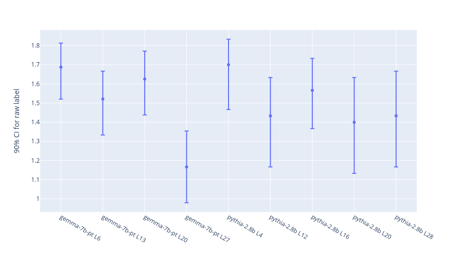
Figure 18: Per-layer 90% confidence intervals for the mean interpretability label

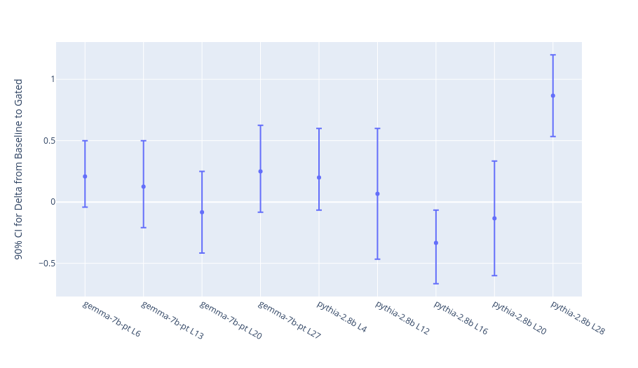
Figure 19: Per-layer 90% confidence intervals for the Gated-vs-Baseline label difference

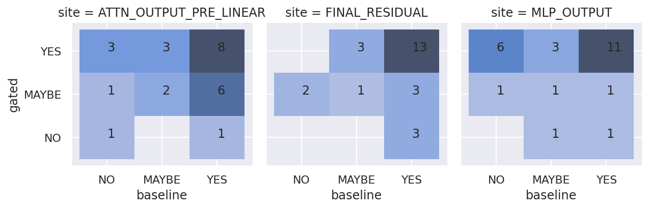
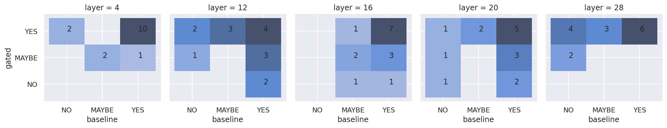
Figure 20: Contingency tables for the paired (gated vs baseline) interpretability labels, for Pythia-2.8B

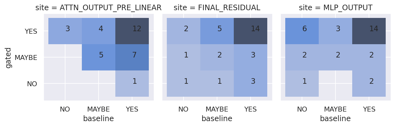
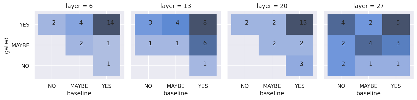
Figure 21: Contingency tables for the paired (gated vs baseline) interpretability labels, for Gemma-7B

H.3 Raters

In Table 10 we present test results weakly suggesting that the raters differed in their judgments. This underscores that there’s still a significant subjective component to this interpretability labeling. (Notably, different raters saw different proportions of Pythia vs Gemma features, so aggregating across the models is partially confounded by that.)

$p$-values	Raw label	Delta from Baseline to Gated
Across models (Kruskal-Wallis H-test)	.01	.71
Pythia-2.8B (Friedman test)	.13	.05
Gemma-7B (Friedman test)	.03	.76

Table 10: Rater significance tests

References

- Aharon et al. (2006) M. Aharon, M. Elad, and A. Bruckstein. K-svd: An algorithm for designing overcomplete dictionaries for sparse representation. IEEE Transactions on Signal Processing, 54(11):4311–4322, 2006. 10.1109/TSP.2006.881199.
- Anthropic AI (2024) Anthropic AI. Introducing the next generation of Claude. https://www.anthropic.com/index/introducing-the-next-generation-of-claude, 2024. Accessed: 2024-04-14.
- Batson et al. (2024) J. Batson, B. Chen, A. Jones, A. Templeton, T. Conerly, J. Marcus, T. Henighan, N. L. Turner, and A. Pearce. Circuits Updates - March 2024. Transformer Circuits Thread, 2024. URL https://transformer-circuits.pub/2024/mar-update/index.html.
- Bengio (2013) Y. Bengio. Deep learning of representations: Looking forward, 2013.
- Biderman et al. (2023) S. Biderman, H. Schoelkopf, Q. G. Anthony, H. Bradley, K. O’Brien, E. Hallahan, M. A. Khan, S. Purohit, U. S. Prashanth, E. Raff, et al. Pythia: A suite for analyzing large language models across training and scaling. In International Conference on Machine Learning, pages 2397–2430. PMLR, 2023.
- Bills et al. (2023) S. Bills, N. Cammarata, D. Mossing, H. Tillman, L. Gao, G. Goh, I. Sutskever, J. Leike, J. Wu, and W. Saunders. Language models can explain neurons in language models. https://openaipublic.blob.core.windows.net/neuron-explainer/paper/index.html, 2023.
- Bloom (2024) J. Bloom. Open Source Sparse Autoencoders for all Residual Stream Layers of GPT-2 Small. https://www.alignmentforum.org/posts/f9EgfLSurAiqRJySD/open-source-sparse-autoencoders-for-all-residual-stream, 2024.
- Blumensath and Davies (2008) T. Blumensath and M. E. Davies. Gradient pursuits. IEEE Transactions on Signal Processing, 56(6):2370–2382, 2008.
- Bolukbasi et al. (2021) T. Bolukbasi, A. Pearce, A. Yuan, A. Coenen, E. Reif, F. Viégas, and M. Wattenberg. An interpretability illusion for bert. arXiv preprint arXiv:2104.07143, 2021.
- Bricken et al. (2023) T. Bricken, A. Templeton, J. Batson, B. Chen, A. Jermyn, T. Conerly, N. Turner, C. Anil, C. Denison, A. Askell, R. Lasenby, Y. Wu, S. Kravec, N. Schiefer, T. Maxwell, N. Joseph, Z. Hatfield-Dodds, A. Tamkin, K. Nguyen, B. McLean, J. E. Burke, T. Hume, S. Carter, T. Henighan, and C. Olah. Towards monosemanticity: Decomposing language models with dictionary learning. Transformer Circuits Thread, 2023. https://transformer-circuits.pub/2023/monosemantic-features/index.html.
- Chen et al. (2018) R. T. Chen, X. Li, R. B. Grosse, and D. K. Duvenaud. Isolating sources of disentanglement in variational autoencoders. Advances in neural information processing systems, 31, 2018.
- Chen et al. (2016) X. Chen, Y. Duan, R. Houthooft, J. Schulman, I. Sutskever, and P. Abbeel. Infogan: Interpretable representation learning by information maximizing generative adversarial nets. Advances in neural information processing systems, 29, 2016.
- Conmy (2023) A. Conmy. My best guess at the important tricks for training 1L SAEs. https://www.lesswrong.com/posts/yJsLNWtmzcgPJgvro/my-best-guess-at-the-important-tricks-for-training-1l-saes, Dec 2023.
- Conmy et al. (2023) A. Conmy, A. N. Mavor-Parker, A. Lynch, S. Heimersheim, and A. Garriga-Alonso. Towards automated circuit discovery for mechanistic interpretability, 2023.
- Cunningham et al. (2023) H. Cunningham, A. Ewart, L. Riggs, R. Huben, and L. Sharkey. Sparse autoencoders find highly interpretable features in language models, 2023.
- Dauphin et al. (2017) Y. N. Dauphin, A. Fan, M. Auli, and D. Grangier. Language modeling with gated convolutional networks. In Proceedings of the 34th International Conference on Machine Learning - Volume 70, ICML’17, page 933–941. JMLR.org, 2017.
- Elad (2010) M. Elad. Sparse and Redundant Representations: From Theory to Applications in Signal and Image Processing. Springer, New York, 2010. ISBN 978-1-4419-7010-7. 10.1007/978-1-4419-7011-4.
- Elhage et al. (2021) N. Elhage, N. Nanda, C. Olsson, T. Henighan, N. Joseph, B. Mann, A. Askell, Y. Bai, A. Chen, T. Conerly, N. DasSarma, D. Drain, D. Ganguli, Z. Hatfield-Dodds, D. Hernandez, A. Jones, J. Kernion, L. Lovitt, K. Ndousse, D. Amodei, T. Brown, J. Clark, J. Kaplan, S. McCandlish, and C. Olah. A mathematical framework for transformer circuits. Transformer Circuits Thread, 2021. URL https://transformer-circuits.pub/2021/framework/index.html.
- Elhage et al. (2022a) N. Elhage, T. Hume, C. Olsson, N. Nanda, T. Henighan, S. Johnston, S. ElShowk, N. Joseph, N. DasSarma, B. Mann, D. Hernandez, A. Askell, K. Ndousse, A. Jones, D. Drain, A. Chen, Y. Bai, D. Ganguli, L. Lovitt, Z. Hatfield-Dodds, J. Kernion, T. Conerly, S. Kravec, S. Fort, S. Kadavath, J. Jacobson, E. Tran-Johnson, J. Kaplan, J. Clark, T. Brown, S. McCandlish, D. Amodei, and C. Olah. Softmax linear units. Transformer Circuits Thread, 2022a. https://transformer-circuits.pub/2022/solu/index.html.
- Elhage et al. (2022b) N. Elhage, T. Hume, C. Olsson, N. Schiefer, T. Henighan, S. Kravec, Z. Hatfield-Dodds, R. Lasenby, D. Drain, C. Chen, et al. Toy Models of Superposition. arXiv preprint arXiv:2209.10652, 2022b.
- Erichson et al. (2019) N. B. Erichson, Z. Yao, and M. W. Mahoney. Jumprelu: A retrofit defense strategy for adversarial attacks, 2019.
- Gemini Team (2024) Gemini Team. Gemini: A Family of Highly Capable Multimodal Models. Rohan Anil and Sebastian Borgeaud and Yonghui Wu and Jean-Baptiste Alayrac and Jiahui Yu and Radu Soricut and Johan Schalkwyk and Andrew M Dai and Anja Hauth et. al, 2024.
- Gemma Team et al. (2024) Gemma Team, T. Mesnard, C. Hardin, R. Dadashi, S. Bhupatiraju, L. Sifre, M. Rivière, M. S. Kale, J. Love, P. Tafti, L. Hussenot, and et al. Gemma, 2024. URL https://www.kaggle.com/m/3301.
- Gurnee and Tegmark (2024) W. Gurnee and M. Tegmark. Language models represent space and time, 2024.
- Gurnee et al. (2023) W. Gurnee, N. Nanda, M. Pauly, K. Harvey, D. Troitskii, and D. Bertsimas. Finding neurons in a haystack: Case studies with sparse probing, 2023.
- Hastie et al. (2015) T. Hastie, R. Tibshirani, and M. Wainwright. Statistical Learning with Sparsity: The Lasso and Generalizations. CRC Press, Boca Raton, FL, 2015. ISBN 978-1-4987-1216-3. 10.1201/b18401.
- Kim and Mnih (2018) H. Kim and A. Mnih. Disentangling by factorising. In International conference on machine learning, pages 2649–2658. PMLR, 2018.
- Kissane et al. (2024a) C. Kissane, R. Krzyzanowski, A. Conmy, and N. Nanda. Sparse autoencoders work on attention layer outputs. Alignment Forum, 2024a. URL https://www.alignmentforum.org/posts/DtdzGwFh9dCfsekZZ.
- Kissane et al. (2024b) C. Kissane, R. Krzyzanowski, A. Conmy, and N. Nanda. Attention saes scale to gpt-2 small. Alignment Forum, 2024b. URL https://www.alignmentforum.org/posts/FSTRedtjuHa4Gfdbr.
- Mallat and Zhang (1993) S. Mallat and Z. Zhang. Matching pursuits with time-frequency dictionaries. IEEE Transactions on Signal Processing, 41(12):3397–3415, 1993. 10.1109/78.258082.
- Marks et al. (2024) S. Marks, C. Rager, E. J. Michaud, Y. Belinkov, D. Bau, and A. Mueller. Sparse feature circuits: Discovering and editing interpretable causal graphs in language models, 2024.
- Mathieu et al. (2019) E. Mathieu, T. Rainforth, N. Siddharth, and Y. W. Teh. Disentangling disentanglement in variational autoencoders. In International conference on machine learning, pages 4402–4412. PMLR, 2019.
- McDougall (2024) C. McDougall. SAE Visualizer. https://github.com/callummcdougall/sae_vis, 2024.
- McDougall et al. (2023) C. McDougall, A. Conmy, C. Rushing, T. McGrath, and N. Nanda. Copy suppression: Comprehensively understanding an attention head, 2023.
- Nanda (2022) N. Nanda. My Interpretability-Friendly Models (in TransformerLens). https://dynalist.io/d/n2ZWtnoYHrU1s4vnFSAQ519J#z=NCJ6zH_Okw_mUYAwGnMKsj2m, 2022.
- Nanda (2023) N. Nanda. Open Source Replication & Commentary on Anthropic’s Dictionary Learning Paper, Oct 2023. URL https://www.alignmentforum.org/posts/aPTgTKC45dWvL9XBF/open-source-replication-and-commentary-on-anthropic-s.
- Nanda et al. (2023) N. Nanda, L. Chan, T. Lieberum, J. Smith, and J. Steinhardt. Progress measures for grokking via mechanistic interpretability. In The Eleventh International Conference on Learning Representations, 2023. URL https://openreview.net/forum?id=9XFSbDPmdW.
- Nanda et al. (2024) N. Nanda, A. Conmy, L. Smith, S. Rajamanoharan, T. Lieberum, J. Kramár, and V. Varma. [Summary] Progress Update #1 from the GDM Mech Interp Team. Alignment Forum, 2024. URL https://www.alignmentforum.org/posts/HpAr8k74mW4ivCvCu/summary-progress-update-1-from-the-gdm-mech-interp-team.
- Ng (2011) A. Ng. Sparse autoencoder. http://web.stanford.edu/class/cs294a/sparseAutoencoder.pdf, 2011. CS294A Lecture notes.
- Olah (2022) C. Olah. Mechanistic interpretability, variables, and the importance of interpretable bases. https://www.transformer-circuits.pub/2022/mech-interp-essay, 2022.
- Olah et al. (2020) C. Olah, N. Cammarata, L. Schubert, G. Goh, M. Petrov, and S. Carter. Zoom in: An introduction to circuits. Distill, 2020. 10.23915/distill.00024.001.
- Olah et al. (2023) C. Olah, T. Bricken, J. Batson, A. Templeton, A. Jermyn, T. Hume, and T. Henighan. Circuits Updates - May 2023. Transformer Circuits Thread, 2023. URL https://transformer-circuits.pub/2023/may-update/index.html.
- Olah et al. (2024) C. Olah, S. Carter, A. Jermyn, J. Batson, T. Henighan, T. Conerly, J. Marcus, A. Templeton, B. Chen, and N. L. Turner. Circuits Updates - January 2024. Transformer Circuits Thread, 2024. URL https://transformer-circuits.pub/2024/jan-update/index.html.
- Olshausen and Field (1997) B. A. Olshausen and D. J. Field. Sparse coding with an overcomplete basis set: A strategy employed by v1? Vision Research, 37(23):3311–3325, 1997. 10.1016/S0042-6989(97)00169-7.
- Olsson et al. (2022) C. Olsson, N. Elhage, N. Nanda, N. Joseph, N. DasSarma, T. Henighan, B. Mann, A. Askell, Y. Bai, A. Chen, et al. In-context learning and induction heads, 2022. URL https://transformer-circuits.pub/2022/in-context-learning-and-induction-heads/index.html.
- OpenAI (2023) OpenAI. GPT-4 Technical Report, 2023.
- Park et al. (2023) K. Park, Y. J. Choe, and V. Veitch. The linear representation hypothesis and the geometry of large language models, 2023.
- Pati et al. (1993) Y. Pati, R. Rezaiifar, and P. Krishnaprasad. Orthogonal matching pursuit: recursive function approximation with applications to wavelet decomposition. In Proceedings of 27th Asilomar Conference on Signals, Systems and Computers, pages 40–44 vol.1, 1993. 10.1109/ACSSC.1993.342465.
- Sharkey et al. (2022) L. Sharkey, D. Braun, and B. Millidge. [interim research report] taking features out of superposition with sparse autoencoders. https://www.alignmentforum.org/posts/z6QQJbtpkEAX3Aojj/interim-research-report-taking-features-out-of-superposition, 2022.
- Shazeer (2020) N. Shazeer. GLU variants improve transformer. CoRR, abs/2002.05202, 2020. URL https://arxiv.org/abs/2002.05202.
- Sundararajan et al. (2017) M. Sundararajan, A. Taly, and Q. Yan. Axiomatic attribution for deep networks. In D. Precup and Y. W. Teh, editors, Proceedings of the 34th International Conference on Machine Learning, ICML 2017, Sydney, NSW, Australia, 6-11 August 2017, volume 70 of Proceedings of Machine Learning Research, pages 3319–3328. PMLR, 2017. URL http://proceedings.mlr.press/v70/sundararajan17a.html.
- Taggart (2024) G. M. Taggart. Prolu: A nonlinearity for sparse autoencoders. https://www.lesswrong.com/posts/HEpufTdakGTTKgoYF/prolu-a-pareto-improvement-for-sparse-autoencoders, 2024.
- Tamkin et al. (2023) A. Tamkin, M. Taufeeque, and N. D. Goodman. Codebook features: Sparse and discrete interpretability for neural networks, 2023.
- Templeton et al. (2024) A. Templeton, J. Batson, T. Henighan, T. Conerly, J. Marcus, A. Golubeva, T. Bricken, and A. Jermyn. Circuits Updates - February 2024. Transformer Circuits Thread, 2024. URL https://transformer-circuits.pub/2024/feb-update/index.html.
- Thorpe (1989) S. J. Thorpe. Local vs. distributed coding. Intellectica, 8:3–40, 1989.
- Tibshirani (1996) R. Tibshirani. Regression shrinkage and selection via the lasso. Journal of the Royal Statistical Society: Series B (Methodological), 58(1):267–288, 1996. 10.1111/j.2517-6161.1996.tb02080.x.
- Tigges et al. (2023) C. Tigges, O. J. Hollinsworth, A. Geiger, and N. Nanda. Linear representations of sentiment in large language models, 2023.
- Turner et al. (2023) A. M. Turner, L. Thiergart, D. Udell, G. Leech, U. Mini, and M. MacDiarmid. Activation addition: Steering language models without optimization, 2023.
- Wang et al. (2023) K. R. Wang, A. Variengien, A. Conmy, B. Shlegeris, and J. Steinhardt. Interpretability in the wild: a circuit for indirect object identification in GPT-2 small. In The Eleventh International Conference on Learning Representations, 2023. URL https://openreview.net/forum?id=NpsVSN6o4ul.
- Wright and Sharkey (2024) B. Wright and L. Sharkey. Addressing feature suppression in saes. https://www.alignmentforum.org/posts/3JuSjTZyMzaSeTxKk/addressing-feature-suppression-in-saes, Feb 2024.
- Yun et al. (2023) Z. Yun, Y. Chen, B. A. Olshausen, and Y. LeCun. Transformer visualization via dictionary learning: contextualized embedding as a linear superposition of transformer factors, 2023.