Generation of bipartite mechanical cat state by performing projective Bell state measurement.
Abstract
Quantum state preparation and measurement of photonic and phononic Schrödinger cat states have gathered significant interest due to their implications for alternative encoding schemes in quantum computation. These scheme employ coherent state superpositions, leveraging the expanded Hilbert space provided by cavity or mechanical resonators in contrast to two-level systems. Moreover, such cat states also serve as a platform for testing fundamental quantum phenomena in macroscopic systems. In this study, we generate four bipartite phononic Bell cat states using an entanglement swapping scheme achieved through projective Bell state measurements on two superconducting qubits. Subsequently, we conduct a Bell inequality test on the bipartite cat state using the CHSH formulation. Given that the entangled cat states are generated through entanglement swapping, our approach could hold promising applications for the advancement of complex quantum network processors based on continuous variable systems.
I Introduction
Observing the quantum behaviour of macroscopic mechanical structures continues to be a challenging endeavour and a significant step towards realizing quantum-acoustic state preparation and measurement. The intriguing aspect of these structures, being massive yet displaying quantum behaviour, makes them important platforms for implementing various quantum technological applications and for exploring fundamental physics questions. Recent experiments have unequivocally demonstrated the quantum properties of solid-state mechanical objects [1, 2, 3, 4, 5, 6]. These include interfacing mechanical objects with the strong quantum nonlinearity of superconducting qubits, leading to the field of circuit quantum acoustodynamics (cQAD) [7, 8, 9, 10, 11, 12, 13] which is analogous to the well-developed field of circuit quantum electrodynamics (cQED) [14, 15, 16]. The integration of superconducting qubits serves as a quantum-acoustic state preparation and measurement element for the mechanical system [12, 17]. These state preparations and measurements are some of the basic building blocks for constructing acoustic quantum memories and processors.
A very significant quantum-acoustic state that can be prepared from the superconducting qubit-mechanical integrated system is the phononic Schrödinger cat state, defined as quantum superpositions of quasi-classical coherent states. Such phononic cat state preparation has been studied in [18, 19]. Similar photonic cat states have also been studied in other various quantum systems such as circuit quantum electrodynamics [20, 21], vibrational states of trapped ions [22], propagating photon modes [23, 24]. Preparing cat states has attracted wide research attention owing to its applications in implementing quantum metrology [25] and quantum information processing protocols based on continuous-variable cat states [26], as well as testing fundamental quantum phenomena in macroscopic systems [27]. One of the most fundamental tests of quantum phenomena in a quantum system is the Bell inequality test [28, 29, 30, 31]. Bell inequality tests, performed on pairs of spatially separated entangled quantum systems, demonstrate that quantum systems do not adhere to the principle of local causality. In this work, we use the Clauser–Horne–Shimony–Holt (CHSH) [32] formulation of the Bell test to conduct the Bell inequality test on a bipartite entangled phononic cat state generated through projective Bell state measurement on a pair of superconducting qubits [33]. The creation of bipartite cat states is demonstrated in photonic resonators [21, 34]. In our scheme, four bipartite phononic cat states, or four phononic Bell states, are generated on two phononic crystal mechanical resonators, interacting piezoelectrically with a pair of superconducting qubits via capacitive coupling. The two qubits are connected through a microwave cavity resonator, and through virtual excitation of the cavity photon, they become entangled, creating qubit Bell state. Upon projective measurement of the Bell state of the qubits, each of the four bipartite phononic cat states can be distinguished. This measurement effectively swaps the entanglement from qubit-mechanical to mechanical-mechanical pairs. Such entanglement swapping schemes are pivotal in quantum repeaters, essential for realizing long-distance quantum communication and complex quantum networks [35, 36, 37]. Since the two qubits are connected via a microwave cavity bus, the phononic crystal resonator can be placed at far ends, enabling long-distance quantum state preparation. By harnessing this capability and employing entanglement swapping schemes, the bipartite phononic cat states generated in this study hold promise for practical applications in implementing quantum network processors relying on continuous variable resonators.
We begin in Section II with a brief introduction of the hybrid electromechanical system under study and then discuss the generation of resonator-qubit Bell cat state. In Section III, we examine the projective Bell state measurement on the two qubits, which leads to entanglement swapping from qubit-qubit to resonator-resonator. We show how this Bell state measurement is realized and how four bipartite phononic Bell cat states are created as a result of the projective measurement. Moving on to Section IV, we conduct the Bell inequality test on the bipartite cat state using the CHSH formulation.
II Qubit-mechanical resonator entanglement.
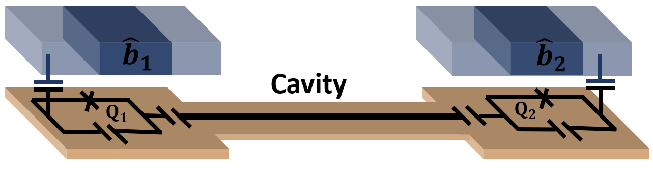
We consider two hybrid electromechanical systems, each comprising a mechanical resonator dispersively coupled to a superconducting qubit as shown in Fig. 1. Assuming that the two qubit-mechanical pairs are uncoupled (appendix A), the Hamiltonian of the two hybrid systems reads as
| (1a) | |||||
| (1b) | |||||
Here, ( and are the qubit and mechanical frequency of the first (second) hybrid system. and are the operators of the two mechanical resonators. In the dispersive coupling, the detuning () is much larger than the coupling strength () between the qubit and the mechanical resonator. We prepare two entangled Bell-cat states by evolving the Hamiltonian and . Initiating the qubits in the superposition state and the mechanical resonators in the coherent state, the state of the first hybrid system, after some time , in the interaction frame, becomes
| (2) |
where is the coherent state of the first mechanical resonator, while and refer to the excited and the ground states of the first qubit, respectively. We get a similar state for the second hybrid system. At time interval , where , we get the Bell-cat state of the qubit-mechanical system.
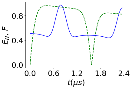
The fidelity and entanglement of the bipartite state in the presence of a noisy environment is shown in Fig. 2. The noisy environment is included by solving the Lindblad master equation.
| (3) | |||||
where with . and are the decay rates of the mechanical resonator and the qubit, respectively. The entanglement of the qubit-mechanical bipartite system is computed using the relation , where is the trace norm of the partial transpose of the bipartite mixed state [39]. As shown in the figure, the fidelity (F) reaches near one at the interval , , and so on for coupling constant MHz. Therefore, the qubit-mechanical bipartite system evolves into a Bell-cat state at the interval of .
III Generation of bipartite cat state.
After the interaction time of , the state of the qubit-mechanical bipartite state (Eq.2) become . The state of the combined system is then given by the tensor product of the states of the two hybrid systems, i.e.,
| (4) | |||||
where is the coherent amplitude of the second resonator. In terms of Bell’s basis, and , the wave function of the combined system (Eq. 4) can be rearranged to
Therefore, by measurement the Bell’s states and , the two mechanical resonators are projected into the bipartite cat states and , respectively. The Bell state measurement of the two qubits is performed by first switching on the interaction between them. This interaction, which will entangle the two qubits, is achieved by red detuning the second qubit from the cavity and blue detuning the same qubit from the second resonator (appendix A). Such detuning arrangement allows the exchange of virtual cavity photons with the qubits. However, this virtual interaction between the two qubits only produces two of the four Bell states, . To generate all four Bell states, we continuously drive the two qubits, resulting in two dressed states. When the difference in the frequencies of the two qubits is much larger than their interaction strength and the phase of the two drives, which is inverted in the middle of the two-qubit interaction, is the same, all four Bell states are generated.
They are mapped onto the computational basis as , , , and [33, 40] (appendix B). Therefore, based on measuring outcomes of the two qubits in the computational basis, all the four bipartite cat states of the resonators are generated.
The above protocol is realized in the noisy environment by first independently evolving the two qubit-mechanical hybrid systems under the Lindblad master equation and then performing the projective measurement on the density matrix of the combined system, . The reduced density matrices of the four bipartite Bell-cat states after the projective Bell state measurement on the two qubits read as,
| (6) | |||||
Constructing the reduced density matrix (Eq. 6) on the number basis will require a huge subspace, and performing joint state tomography on the resonators will be experimentally challenging. So, we construct the density matrix into a two-level system subspace by measuring the displaced phonon number parity observable , where is the displacement operator and the phonon number parity operator [41, 42]. By applying the projector to the displaced parity operator , the Pauli operators for the resonator mode become
| (7) | |||||
We have assumed a large orthonormal cat state, i.e., . The basis for these operators is (, ) which is analogous to the qubit basis (, ). Similar Pauli operators and basis (, ) can be generated for the second resonator using the same approach.
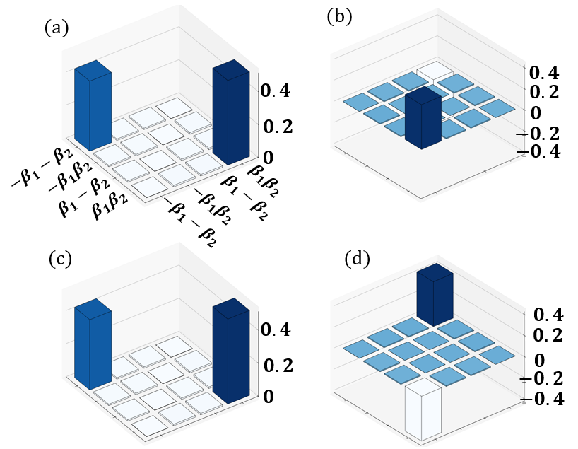
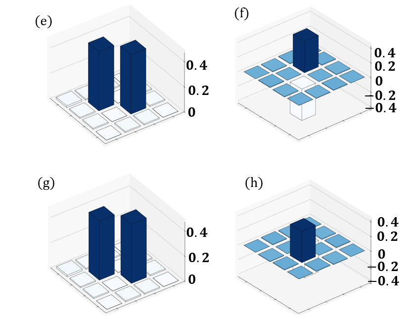
In Fig. 3, we plot the joint density matrix of the two resonators in the joint basis states (, , , and ). We observe four bipartite cat states having fidelities , , , and and entanglements , , , and . The dip in the density matrix element is attributed to the decoherence effect of the two qubits and the relaxation of the two resonators. In addition to the decays resulting from direct contact with the noisy environment, the other factors that lead to the infidelities of the prepared state include read-out errors and errors while performing the Bell measurement. The four bipartite cat states resemble the traditional qubit Bell states generated using a Hadamard and CNOT gate in a quantum circuit. Going by this similarity, the scheme proposed here could be used to implement an entanglement gate for a continuous variable resonator qubit, and may find applications in the bosonic based quantum processors.
IV Bell’s test of the resonator bipartite cat state
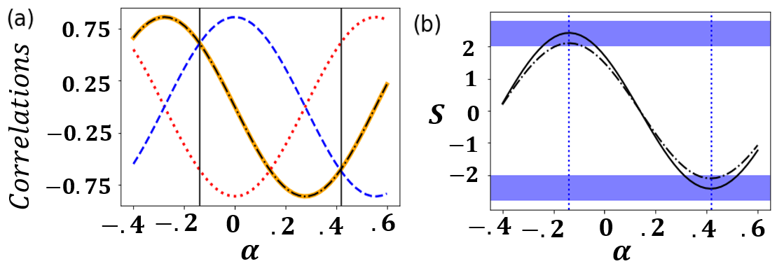
The bipartite entangled cat states of the two resonators generated on a conditional Bell state measurement of the two qubits can be used as a platform to test the Bell’s inequality in a macroscopic quantum system. Here, we perform this test by calculating the expectation values of all the correlations of the measurement outcomes measured locally at the two resonators and then determine the Clauser–Horne–Shimony–Holt (CHSH) value , where, () and () are the observables of the first (second) resonator. The observables are measured in the resonator qubit subspace discussed above. As per CHSH inequality, a system is said to be classically correlated if and quantumly if . The correlation of the observables is measured by first choosing two arbitrary values of and corresponding to , and , , respectively. We then rotate the resonator detector basis by coherently displacing the observables and to and or
| (8) | |||||
Here, is the coherent displacement amplitude of the resonator. By changing the amplitude , we are able to rotate the measurement basis direction and perform measurements at all possible orientations of the detectors. The value for the state is shown in Fig. 4. We observe maximum value when and at the displacement amplitude and . Furthermore, the , and amplitudes corresponding to the maximum value satisfy the relations and . The corresponding observables (Eq. 8) at these amplitudes become and . Therefore, the value observed in the figure exceeds the classical bound limit and attains a maximum of 2.44, which is less than the ideal quantum bound limit . As we increase the decay rates of the resonators, the maximum attainable value decreases, as shown in Fig 4(b). The expectation values of all the measurement correlations are also shown in Fig. 4(a). The behaviour of these correlations as we change the displacement amplitude resembles the one observed in two-qubit Bell test experiments [31]. By integrating two phononic crystal resonators into the experimental arrangement typically employed for conducting a loophole-free Bell test with two superconducting qubits [31], our proposed approach could be employed to examine the Bell inequality of a phononic cat state. Additionally, the bipartite phononic cat state generated through entanglement swapping in this work could hold significant practical implications for the advancement of complex quantum network processors based on continuous variable resonators.
V Conclusion
In conclusion, we propose a scheme to generate four bipartite phononic cat states by performing a projective Bell state measurement on two superconducting qubits. Initially uncoupled phononic crystal resonators, each coupled to a different superconducting qubit, become entangled through entanglement swapping from qubit-mechanical to mechanical-mechanical interactions. Displaced phonon parity measurement is done for generating joint density matrix of the two resonators in two-level subspace. These joint density matrices resemble those of traditional qubit Bell states generated using a Hadamard and CNOT gate in a quantum circuit. Subsequently, we investigate the Bell inequality test using the CHSH formulation. The expectation values of the measurement correlations and the values of the CHSH inequality test obtained here are akin to those observed in [31] for two superconducting qubits. The bipartite phononic cat state generated through entanglement swapping in this work may find useful in implementing quantum network processors based on continuous variable resonators. Furthermore, the scheme presented in this work also serves as a platform for studying Bell inequality test in continuous variable system.
Acknowledgement
R.N. gratefully acknowledges support of a research fellowship from CSIR, Govt. of India. U.D. gratefully acknowledges a research fellowship from MoE, Government of India. A.K.S. acknowledges the STARS scheme, MoE, government of India (Proposal ID 2023-0161).
Appendix A Dispersive Hamiltonian
The interaction part of the complete Hamiltonian, including the cavity resonator connecting the two qubits, is given by the Jaynes-Cummings interaction
| (9) | |||||
Here, and are the coupling strength of mechanical-qubit and qubit-cavity interactions, respectively. and are the creation and annihilation operators of the cavity resonator. We blue detune the first resonator from the first qubit (), second qubit from the cavity resonator (), and red detune the cavity from the first qubit (), second resonator from the second qubit (). Here, refers to the cavity resonance frequency. Because of the detuning, we can transform the Jaynes-Cummings interaction (Eq. A1) into a dispersive one by performing a unitary operation on .
| (10) | |||||
where , , , , , and . The first term in the Hamiltonian A2 can be neglected since the cavity remains in the ground state. By choosing the detuning as , and , we can also neglect the fourth, fifth, and sixth terms [38, 43]. The remaining two interacting terms are the ones used in Hamiltonian 1a and 1b. Thus, we see that by changing the detuning, we can independently evolve the two qubit-resonator pairs. After the two pairs evolve up to a certain time period, we bring back the qubit-qubit interaction (fourth term) to perform Bell state measurement [33]. This can be done in two ways. First, by choosing , or second, by red detuning the second qubit from the cavity and blue detuning the second qubit from the second resonator. In the second approach the coupling constant becomes , where . The rearrangement of the detuning in the second approach ensures that the last term in the Hamiltonian 10 remains zero. This interaction allows us to perform the necessary Bell test on the two qubits.
Appendix B Bell State of the two qubits
In order to distinguish all the Bell states of the two qubit, we resonantly drive the qubits individually. In the interaction frame, the Hamiltonian of the two qubit inteaction is
| (11) |
Here, and are the Rabi frequency and phase, respectively, of the drive applied to the qubits. We have assumed that . The drive produces two dressed states . The qubit cannot go into transitions between different dressed states under the conditions and . Then the Hamiltonian 11 in the dressed state basis reduces to [40, 33].
| (12) |
Here, . If the phases of both the driving fields are reversed right in the middle of the two-qubit interaction time, then the dressed state evolves to . At time , the dressed state become . In the computational basis (, ), the state can be obtained by applying the unitary operator
| (13) |
Therefore, in the computational basis the Bell state is mapped to , i.e., . Similarly, , , and are mapped onto , , .
References
- O’Connell et al. [2010] A. D. O’Connell, M. Hofheinz, M. Ansmann, R. C. Bialczak, M. Lenander, E. Lucero, M. Neeley, D. Sank, H. Wang, M. Weides, et al., Nature 464, 697 (2010).
- Arrangoiz-Arriola et al. [2019] P. Arrangoiz-Arriola, E. A. Wollack, Z. Wang, M. Pechal, W. Jiang, T. P. McKenna, J. D. Witmer, R. Van Laer, and A. H. Safavi-Naeini, Nature 571, 537 (2019).
- Chu et al. [2018] Y. Chu, P. Kharel, T. Yoon, L. Frunzio, P. T. Rakich, and R. J. Schoelkopf, Nature 563, 666 (2018).
- Kotler et al. [2021] S. Kotler, G. A. Peterson, E. Shojaee, F. Lecocq, K. Cicak, A. Kwiatkowski, S. Geller, S. Glancy, E. Knill, R. W. Simmonds, et al., Science 372, 622 (2021).
- Ockeloen-Korppi et al. [2018] C. Ockeloen-Korppi, E. Damskägg, J.-M. Pirkkalainen, M. Asjad, A. Clerk, F. Massel, M. Woolley, and M. Sillanpää, Nature 556, 478 (2018).
- MacCabe et al. [2020] G. S. MacCabe, H. Ren, J. Luo, J. D. Cohen, H. Zhou, A. Sipahigil, M. Mirhosseini, and O. Painter, Science 370, 840 (2020).
- Pirkkalainen et al. [2013] J.-M. Pirkkalainen, S. Cho, J. Li, G. Paraoanu, P. Hakonen, and M. Sillanpää, Nature 494, 211 (2013).
- Lecocq et al. [2015] F. Lecocq, J. D. Teufel, J. Aumentado, and R. W. Simmonds, Nature Physics 11, 635 (2015).
- Bienfait et al. [2019] A. Bienfait, K. J. Satzinger, Y. Zhong, H.-S. Chang, M.-H. Chou, C. R. Conner, É. Dumur, J. Grebel, G. A. Peairs, R. G. Povey, et al., Science 364, 368 (2019).
- LaHaye et al. [2009] M. LaHaye, J. Suh, P. Echternach, K. C. Schwab, and M. L. Roukes, Nature 459, 960 (2009).
- Lee et al. [2023] N. R. Lee, Y. Guo, A. Y. Cleland, E. A. Wollack, R. G. Gruenke, T. Makihara, Z. Wang, T. Rajabzadeh, W. Jiang, F. M. Mayor, P. Arrangoiz-Arriola, C. J. Sarabalis, and A. H. Safavi-Naeini, PRX Quantum 4, 040342 (2023).
- Wollack et al. [2022a] E. A. Wollack, A. Y. Cleland, R. G. Gruenke, Z. Wang, P. Arrangoiz-Arriola, and A. H. Safavi-Naeini, Nature 604, 463 (2022a).
- Von Lüpke et al. [2022a] U. Von Lüpke, Y. Yang, M. Bild, L. Michaud, M. Fadel, and Y. Chu, Nature Physics 18, 794 (2022a).
- Blais et al. [2021] A. Blais, A. L. Grimsmo, S. M. Girvin, and A. Wallraff, Rev. Mod. Phys. 93, 025005 (2021).
- Wallraff et al. [2004] A. Wallraff, D. I. Schuster, A. Blais, L. Frunzio, R.-S. Huang, J. Majer, S. Kumar, S. M. Girvin, and R. J. Schoelkopf, Nature 431, 162 (2004).
- Blais et al. [2007] A. Blais, J. Gambetta, A. Wallraff, D. I. Schuster, S. M. Girvin, M. H. Devoret, and R. J. Schoelkopf, Phys. Rev. A 75, 032329 (2007).
- Von Lüpke et al. [2022b] U. Von Lüpke, Y. Yang, M. Bild, L. Michaud, M. Fadel, and Y. Chu, Nature Physics 18, 794 (2022b).
- Radić et al. [2022] D. Radić, S.-J. Choi, H. C. Park, J. Suh, R. I. Shekhter, and L. Y. Gorelik, npj quantum information 8, 74 (2022).
- Bild et al. [2023] M. Bild, M. Fadel, Y. Yang, U. Von Lüpke, P. Martin, A. Bruno, and Y. Chu, Science 380, 274 (2023).
- Vlastakis et al. [2013] B. Vlastakis, G. Kirchmair, Z. Leghtas, S. E. Nigg, L. Frunzio, S. M. Girvin, M. Mirrahimi, M. H. Devoret, and R. J. Schoelkopf, Science 342, 607 (2013).
- Wang et al. [2016] C. Wang, Y. Y. Gao, P. Reinhold, R. W. Heeres, N. Ofek, K. Chou, C. Axline, M. Reagor, J. Blumoff, K. Sliwa, et al., Science 352, 1087 (2016).
- Wineland [2013] D. J. Wineland, Rev. Mod. Phys. 85, 1103 (2013).
- Hacker et al. [2019] B. Hacker, S. Welte, S. Daiss, A. Shaukat, S. Ritter, L. Li, and G. Rempe, Nature Photonics 13, 110 (2019).
- Ourjoumtsev et al. [2006] A. Ourjoumtsev, R. Tualle-Brouri, J. Laurat, and P. Grangier, Science 312, 83 (2006).
- Tatsuta et al. [2019] M. Tatsuta, Y. Matsuzaki, and A. Shimizu, Phys. Rev. A 100, 032318 (2019).
- Guillaud and Mirrahimi [2019] J. Guillaud and M. Mirrahimi, Phys. Rev. X 9, 041053 (2019).
- Vlastakis et al. [2015a] B. Vlastakis, A. Petrenko, N. Ofek, L. Sun, Z. Leghtas, K. Sliwa, Y. Liu, M. Hatridge, J. Blumoff, L. Frunzio, et al., Nature communications 6, 8970 (2015a).
- Hensen et al. [2015] B. Hensen, H. Bernien, A. E. Dréau, A. Reiserer, N. Kalb, M. S. Blok, J. Ruitenberg, R. F. Vermeulen, R. N. Schouten, C. Abellán, et al., Nature 526, 682 (2015).
- Giustina et al. [2015] M. Giustina, M. A. M. Versteegh, S. Wengerowsky, J. Handsteiner, A. Hochrainer, K. Phelan, F. Steinlechner, J. Kofler, J.-A. Larsson, C. Abellán, W. Amaya, V. Pruneri, M. W. Mitchell, J. Beyer, T. Gerrits, A. E. Lita, L. K. Shalm, S. W. Nam, T. Scheidl, R. Ursin, B. Wittmann, and A. Zeilinger, Phys. Rev. Lett. 115, 250401 (2015).
- Shalm et al. [2015] L. K. Shalm, E. Meyer-Scott, B. G. Christensen, P. Bierhorst, M. A. Wayne, M. J. Stevens, T. Gerrits, S. Glancy, D. R. Hamel, M. S. Allman, K. J. Coakley, S. D. Dyer, C. Hodge, A. E. Lita, V. B. Verma, C. Lambrocco, E. Tortorici, A. L. Migdall, Y. Zhang, D. R. Kumor, W. H. Farr, F. Marsili, M. D. Shaw, J. A. Stern, C. Abellán, W. Amaya, V. Pruneri, T. Jennewein, M. W. Mitchell, P. G. Kwiat, J. C. Bienfang, R. P. Mirin, E. Knill, and S. W. Nam, Phys. Rev. Lett. 115, 250402 (2015).
- Storz et al. [2023] S. Storz, J. Schär, A. Kulikov, P. Magnard, P. Kurpiers, J. Lütolf, T. Walter, A. Copetudo, K. Reuer, A. Akin, et al., Nature 617, 265 (2023).
- Clauser et al. [1969] J. F. Clauser, M. A. Horne, A. Shimony, and R. A. Holt, Phys. Rev. Lett. 23, 880 (1969).
- Ning et al. [2019] W. Ning, X.-J. Huang, P.-R. Han, H. Li, H. Deng, Z.-B. Yang, Z.-R. Zhong, Y. Xia, K. Xu, D. Zheng, and S.-B. Zheng, Phys. Rev. Lett. 123, 060502 (2019).
- Wang et al. [2022] Z. Wang, Z. Bao, Y. Wu, Y. Li, W. Cai, W. Wang, Y. Ma, T. Cai, X. Han, J. Wang, et al., Science advances 8, eabn1778 (2022).
- Sangouard et al. [2010] N. Sangouard, C. Simon, N. Gisin, J. Laurat, R. Tualle-Brouri, and P. Grangier, JOSA B 27, A137 (2010).
- Mastriani [2023] M. Mastriani, Scientific Reports 13, 21998 (2023).
- Shchukin and van Loock [2022] E. Shchukin and P. van Loock, Phys. Rev. Lett. 128, 150502 (2022).
- Wollack et al. [2022b] E. A. Wollack, A. Y. Cleland, R. G. Gruenke, Z. Wang, P. Arrangoiz-Arriola, and A. H. Safavi-Naeini, Nature 604, 463 (2022b).
- Vidal and Werner [2002] G. Vidal and R. F. Werner, Phys. Rev. A 65, 032314 (2002).
- Guo et al. [2018] Q. Guo, S.-B. Zheng, J. Wang, C. Song, P. Zhang, K. Li, W. Liu, H. Deng, K. Huang, D. Zheng, X. Zhu, H. Wang, C.-Y. Lu, and J.-W. Pan, Phys. Rev. Lett. 121, 130501 (2018).
- Vlastakis et al. [2015b] B. Vlastakis, A. Petrenko, N. Ofek, L. Sun, Z. Leghtas, K. Sliwa, Y. Liu, M. Hatridge, J. Blumoff, L. Frunzio, et al., Nature communications 6, 8970 (2015b).
- Von Lüpke et al. [2022c] U. Von Lüpke, Y. Yang, M. Bild, L. Michaud, M. Fadel, and Y. Chu, Nature Physics 18, 794 (2022c).
- Majer et al. [2007] J. Majer, J. Chow, J. Gambetta, J. Koch, B. Johnson, J. Schreier, L. Frunzio, D. Schuster, A. A. Houck, A. Wallraff, et al., Nature 449, 443 (2007).