Spin Supersolid Phase and Double Magnon-Roton Excitations in a Cobalt-based Triangular Lattice

Abstract

Supersolid is an exotic quantum state of matter that hosts spontaneously the features of both solid and superfluidity, which breaks the lattice translational symmetry and U(1) gauge symmetry. Here we conduct inelastic neutron scattering (INS) measurements and tensor-network calculations on the triangular-lattice cobaltate Na₂BaCo(PO₄)₂, which is proposed in [Xiang et al., Nature 625, 270-275 (2024)] as a quantum magnetic analog of supersolid. We uncover characteristic dynamical signatures, which include distinct magnetic Bragg peaks indicating out-of-plane spin solidity and gapless Goldstone modes corresponding to the in-plane spin superfluidity, offering comprehensive spectroscopic evidence for spin supersolid in Na₂BaCo(PO₄)₂. We also compute spin dynamics of the easy-axis triangular-lattice model, and reveal magnon-roton excitations containing U(1) Goldstone and roton modes associated with the in-plane spin superfluidity, as well as pseudo-Goldstone and roton modes related to the out-of-plane spin solidity, rendering double magnon-roton dispersions in the spin supersolid. Akin to the role of phonon-roton dispersion in shaping the helium thermodynamics, the intriguing magnetic excitations also strongly influence the low-temperature thermodynamics of spin supersolid down to sub-Kelvin regime, explaining the recently observed giant magnetocaloric effect in Na₂BaCo(PO₄)₂.

Introduction.— As a paradigmatic example of frustrated quantum magnet, the triangular-lattice antiferromagnets (TLAF) have garnered significant attention in the past [1, 2, 3]. The perfect isosceles triangular-lattice compounds, including the cobaltate Ba₃CoSb₂O₉ [4, 5, 6, 7, 8, 9, 10], rare-earth triangular compounds such as REMgGaO₄ (with RE = rare earth) [11, 12, 13, 14, 15, 16, 17, 18] and structurally similar compounds ARECh₂ with A = Na, K, Cs, and Ch = O, S, Se [19, 20, 21, 22, 23, 24, 25, 26], have been synthesized recently. There are investigations into possible quantum spin liquid (QSL) [27, 28, 29, 30], fractional magnetization plateau [31, 32, 33], anomalous low-temperature thermodynamics [34, 35], topological phase transitions [16, 18], and exotic spin excitations [36, 37, 38, 13, 14, 39, 25, 40, 26], etc, making the TLAF systems a very intriguing, fertile ground for studying emergent quantum phenomena.

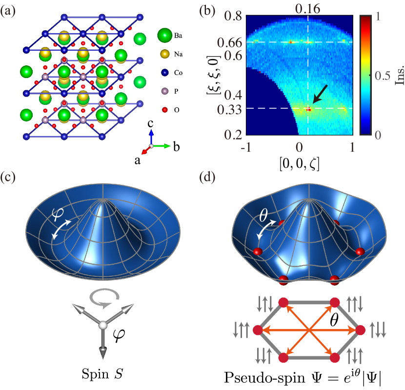
Figure 1: (a) Layered triangular-lattice structure of Na₂BaCo(PO₄)₂, and (b) the elastic scattering results of the measurements. The dashed lines indicate the magnetic propagation vector of $k$ = (1/3, 1/3, 0.16). (c) and (d) The angle $\varphi$ represents the U(1) phase of in-plane spin superfluidity, and $\theta$ is the U(1) phase of the complex order parameter $\Psi$ (i.e., pseudo-spin, see definition in the main text) for the out-of-plane spin solidity. The angles $\varphi$ and $\theta$ are related to the gapless Goldstone and pseudo-Goldstone modes, respectively.

Recently, an easy-axis Co-based triangular-lattice antiferromagnet Na₂BaCo(PO₄)₂ (NBCP) has raised great research interests [41, 42, 43, 44, 45, 46, 47, 48]. The Co²⁺ ions form stacked triangular lattices [c.f., Fig. 1(a)], which carry effective spin $S=1/2$ under the effects of spin-orbit coupling and crystal electric field. The spin-spin couplings are highly two-dimensional, i.e., the intra-layer spin exchanges are dominating over those between the layers [41, 44, 45, 46]. The highly frustrated quantum magnet was first proposed to host a quantum spin liquid, where magnetic ordering was absent down to 300 mK [41, 43]. A later specific heat measurement finds an anomaly at about $T_{\rm N}\simeq 150$ mK [42], which instead suggests the formation of certain spin order at low temperature. The existence of residual thermal conductivity has also been reported in this compound [42], although a different conclusion was drawn based on an independent measurement [47].

An easy-axis TLAF model has been put forward to elucidate the diverse experimental findings in NBCP. The model Hamiltonian reads $H=\sum_{\langle i,j\rangle}J_{xy}(S_{i}^{x}S_{j}^{x}+S_{i}^{y}S_{j}^{y})+J_{z}S_{i}^{z}S_{j}^{z}$, where the nearest-neighbor interactions between $i,j$ are $J_{xy}=0.88{\rm K}$ and $J_{z}=1.48~{}{\rm K}$ [45, 46]. Based on tensor-network calculations on this highly frustrated spin model, it has been proposed theoretically [45] and observed experimentally the long-sought spin supersolidity NBCP, through the magnetocaloric and neutron diffraction measurements [48]. Nevertheless, dynamical features of the spin supersolid phase remain to be unexplored, both in theory and experiment.

Here we conduct INS measurements on single-crystal samples of NBCP down to 55 mK. Complementing these investigations, tensor-network computations are performed using the TLAF model, yielding results that are in excellent agreement with the INS data. This synergy between experimental and theoretical modeling provides a comprehensive understanding of the magnetic properties and dynamics of NBCP at low temperatures. In particular, a substantial downward renormalization is revealed in the magnon dispersion near the M point of Brillouin zone (BZ), constituting the magnetic analog of roton mode. Meanwhile, a pseudo-Goldstone gap is obtained by computing the spin-resolved spectral function. Overall, the peculiar double magnon-roton dispersions, one from in-plane spin superfluidity and the other from out-of-plane spin solidity, render strong spin fluctuations and large magnetic entropies till low temperature and well explain the giant magnetocaloric effect (MCE) observed in NBCP.

Samples and neutron scattering measurements.— Single-crystal samples of Na₂BaCo(PO₄)₂ were grown using the flux method as reported in Ref. 48. The INS experiments were performed on the cold-neutron time-of-flight spectrometer PELICAN [49], at Australian Nuclear Science and Technology Organisation (ANSTO). A total number of 28 pieces of NBCP single crystals with a total mass of about 3 g were mounted on the sample holder made of 6061 aluminum alloy using CYTOP M-type glue. The base temperature of 55 mK was achieved using a dilution insert inside a 7 T vertical cryomagnet. The crystals were co-aligned with their [1, $-$1, 0] direction lying vertically, so that the [$H$, $H$, $L$] scattering plane can be mapped out by rotating the sample and an in-plane magnetic field can be applied along the [1, $-$1, 0] direction.

The instrument was configured with an incident neutron wavelength of $5.96$ Å, providing an incident energy of $2.3$ meV with a high energy resolution of about $0.066$ meV at the elastic line. The dataset below 0.1 meV collected at $2.5$ T was used for background subtraction for the 0 T case, and a standard vanadium sample was measured for detector normalization and determination of the energy resolution function. The data reductions were performed using the software HORACE [50].

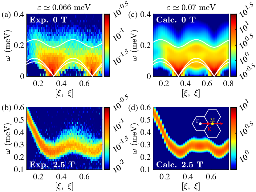
Figure 2: The INS data along the high-symmetry momentum direction, following the path $[\xi,\xi]$ (red arrow) in the reciprocal space shown in the inset of (d), measured under (a) $B=0$ and (b) $B=2.5~{}{\rm T}$ (in-plane field), respectively. Scatterings are integrated along the [$-\eta$, $\eta$, 0] direction perpendicular to the horizontal scattering plane for $\eta$ $\in$ [$-$0.4, 0.4] and along the out-of-plane [0, 0, $\zeta$] direction for $\zeta$ $\in$ [$-$0.2, 0.2]. (c) and (d) show the calculated dynamical spin structure factor $S(k,\omega)=\sum_{\alpha=\{x,y,z\}}S^{\alpha\alpha}(k,\omega)$ under zero and 2.5 T fields, respectively. To simulate the spin dynamics under 2.5 T in-plane field, we include $g_{\rm ab}\mu_{\rm B}B\sum_{i}S_{i}^{x}$, with $\mu_{B}$ the Bohr magneton and the Lande factor $g_{\rm ab}\simeq 4.24$, in the calculations. The white solid lines in (a, c) are the linear spin wave results.

Spectroscopic evidence for spin supersolid.— In Fig. 1(b) we present the elastic scattering ($\omega=0\pm 0.05$ meV) results of the INS measurements, which clearly reveal magnetic Bragg peaks at ${\rm K}\equiv[1/3,1/3]$ points with an incommensurate out-of-plane propagation vector of $\zeta$ = 0.16, due to sensitivity of the spin supersolid state to weak interlayer couplings. Further analysis shows that the magnetic Bragg peaks are contributed mainly from the the out-of-plane moments [51], consistent with prior neutron diffractions results [46, 48]. Besides the magnetic Bragg peaks, the low-energy spin fluctuations observed from the INS measurements exhibit a rod-like shape [51], showing very good two dimensionality of the compound.

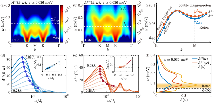
Figure 3: The calculated spin-resolved spectral functions (a) $A^{zz}(k,\omega)$ and (b) $A^{+-}(k,\omega)$ under zero field, with a high energy resolution $\varepsilon\simeq 0.036{\rm meV}$. (c) illustrates the double magnon-roton excitations obtained from $A^{zz}(k,\omega)$ and $A^{+-}(k,\omega)$. The former corresponds to a dispersion with gapless Goldstone mode and roton minimum with gap $\Delta_{\rm R1}\simeq 0.064~{}{\rm meV}$, while the latter has a pseudo-Goldstone mode with gap $\Delta_{\rm PG}$ and roton mode with gap $\Delta_{\rm R2}\simeq 0.07~{}{\rm meV}$. The solid blue circles and red squares are determined from spectral lines in $A^{zz}(k,\omega)$ and $A^{+-}(k,\omega)$, respectively. (d) shows the spectral function $A^{zz}$ at ${\rm K\equiv[1/3,1/3]}$ with different energy resolution $\varepsilon$ ranging from $0.28J_{z}$ (i.e., about 0.036 meV) to $0.08J_{z}$, and the inset shows that the peak position $\Delta_{\rm G}(\varepsilon$) extrapolates to zero as $\varepsilon\rightarrow 0$. (e) depicts the spectral function $A^{+-}(k,\omega)$ at K point with different energy resolution $\varepsilon$, where inset shows the peak location converges to a finite value of $\Delta_{\rm PG}(0)\simeq 0.063J_{z}$. (f) shows the local spectral function $A^{\rm X}(\omega)\equiv\sum_{k}A^{\rm X}(k,\omega)$, with ${\rm X}=zz,+-$ for the in- and out-plane components, and $A(\omega)$ sum of the two.

In Figs. 2(a,b) we present the low-energy magnetic excitations observed at $55~{}{\rm mK}$ with zero field and an in-plane field of $B=2.5~{}{\rm T}$, respectively, and compare them to the model calculations. At zero field, evidence of gapless Goldstone modes are shown in Fig. 2(a), where the linear spin-wave dispersions emanating from the ordering vector ${\rm K}$ are also plotted. The tensor-network calculations with realistic model parameters well reproduce the experimental results with similar energy resolution. On the other hand, with a larger magnetic field $B=2.5~{}{\rm T}$ above the in-plane critical field [42, 45], a clear magnon dispersion in the nearly polarized phase is observed. The theoretical calculations demonstrate an excellent match with the experimental results for both zero and 2.5 T field cases, confirming once again the validity and accuracy of the effective easy-axis TLAF model for NBCP.

Figure 2(a) reveals the presence of an extra intensity that overlays the standard linear spin-wave dispersion, notably concentrated around the $\mathrm{M}\equiv[1/2,1/2]$ high symmetry point of the Brillouin zone. A downward renormalization of magnon dispersion can be discerned in experimental data in Fig. 2(a) and simulated results in Fig. 2(c), which become more evident by improving the energy resolution (see in Fig. 3). Below, we show such soft mode represents magnetic analog of roton excitation in superfluid helium [52, 53, 54, 55, 56].

Dynamical calculations of easy-axis TLAF model.— Here we consider the easy-axis TLAF model with realistic parameters of the spin supersolid compound Na₂BaCo(PO₄)₂ and compute the dynamical spin structure factor $S(k,\omega)$ and spectral function $A(k,\omega)$. These two quantities can be obtained from real-time correlation function $g^{\alpha\beta}(k,t)=\frac{1}{N}e^{{\rm i}E_{0}t}\sum_{i,j}e^{-{{\rm i}k\cdot(r_{i}-r_{j})}}\bra{\psi_{0}}S^{\alpha}_{i}e^{-{\rm i}Ht}S^{\beta}_{j}\ket{\psi_{0}}$, where $\ket{\psi_{0}}$ ($E_{0}$) is the ground-state wavefunction (energy), and $N$ is the total site number. The ground state $\ket{\psi_{0}}$ can be obtained with density matrix renormalization group [57] and the real-time evolution $e^{-{\rm i}Ht}S^{\beta}_{j}\ket{\psi_{0}}$ is computed with time-dependent variational principle approach [58, 59].

Given the correlation function $g^{\alpha\beta}(k,t)$, the spin-resolved dynamical structure factor can be computed as $S^{\alpha\beta}(k,\omega)=\int_{0}^{t_{\rm max}}{\rm Re}[g^{\alpha\beta}(k,t)e^{\rm{i}\omega t}]~{}W({t}/{t_{\rm max}})~{}dt$ and spectral function $A^{\alpha\beta}(k,\omega)=-\int_{0}^{t_{\rm max}}{\rm Im}[g^{\alpha\beta}(k,t)]\sin(\omega t)~{}W({t}/{t_{\rm max}})~{}dt,$ where the energy resolution $\varepsilon$ is controlled by the maximal evolution time $t_{\rm max}$, as $\varepsilon\simeq 8/t_{\rm max}$ with the Parzen window function $W({t}/{t_{\rm max}})$ [51]. In practice, the dynamical calcualtions are performed on a YC$6\times 15$ lattice with the simulated time up to $t_{\max}=100/J_{z}$. For zero-field case, the retained bond dimension is $D=2000$ for all the contour plot with momentum scan, and $D=3000$ for the lines with a fixed momentum [e.g., Fig. 3(d,e)]. For the $B=2.5$ T case, we perform real-time evolutions on a YC$6\times 30$ lattice with bond dimension $D=600$.

In Figs. 3(a,b) we show the results of spin-resolved spectral functions $A^{zz}(k,\omega)$ and $A^{+-}(k,\omega)$, which exhibit distinct behaviors. The spectral functions, rather than the dynamic spin structure factors, are shown in Fig. 3, which do not include the elastic-scattering peaks at ${\rm K}$ and allow us to concentrate on the low-energy fluctuations. From Fig. 3(a) we find that the spectral intensities of $A^{zz}(k,\omega)$ that mainly reflect the in-plane excitations are significant only for $\omega\lesssim 0.15$ meV, i.e., below about $2J_{xy}$. On the other hand, the out-of-plane excitations reflected in $A^{+-}(k,\omega)$ can extend to higher energies of about $0.25~{}{\rm meV}\sim 2J_{z}$. In addition, in Figs. 3(a,b) we find clear single-particle excitations for $0<\omega<J_{xy,z}$ that we dub as magnon-roton dispersions (see discussions below), while for higher energies $J_{xy,z}<\omega<2J_{xy,z}$ both spectra show excitation continuum [51].

Goldstone and pseudo-Goldstone magnons.— To examine the low-energy excitations, we gradually improve the energy resolution to about $0.08J_{z}$ ($t_{\rm max}=100/J_{z}$) in the calculation, and show the results of $A^{zz,+-}(k,\omega)$ in Figs. 3(a,b). where the spectral functions become more coherent as $\varepsilon$ decreases. The spectral function $A^{zz}(k,\omega)$ reflects the in-plane excitations. As the spectral function is parity odd in $\omega$, its peak value $\Delta_{\rm G}$ has been artificially shifted to higher frequencies upon convolution with window functions. As shown in Fig. 3(d), $\Delta_{\rm G}$ becomes lowered as the resolution $\varepsilon$ improves, which extrapolates eventually to approximately zero energy in the $\varepsilon=0$ limit, indicating the existence of gapless Goldstone modes [c.f., Fig. 1(c)].

On the other hand, in Fig. 3(b) we show the low-energy out-of-plane excitations modes by computing the spectral function $A^{+-}({\rm K},\omega)$. As shown in Fig. 3(d), a small but nonzero gap $\Delta_{\rm PG}$ exists, which converge to $\Delta_{\rm PG}\simeq 0.063J_{z}$. This is the pseudo-Goldstone mode that originates from the modified “Mexican-hat” energy landscape with six-fold anisotropy as illustrated in Fig. 1(d). A complex order parameter $\Psi=e^{\rm i\theta}|\Psi|\equiv\frac{1}{N}(\sum_{i\in A}\langle S^{z}_{i}\rangle+\sum_{j\in B}\langle S^{z}_{j}\rangle e^{{\rm i}\pi 2/3}+\sum_{k\in C}\langle S^{z}_{k}\rangle e^{{\rm i}\pi 4/3})$ can be introduced, where $A,B,C$ label the three sublattices and the U(1) phase $\theta$ reveals the “hidden” XY degree of freedom. In Fig. 1(d), the spin configurations like $\uparrow\uparrow\downarrow$ and $\uparrow\downarrow\uparrow$, etc., correspond to the six-fold degenerate ground state with $\theta=n\pi/3$ ($0\leq n\leq 5$). The spin excitations in the vicinities of 6-fold minima cost a finite amount of energy, and this small pseudo-Goldstone gap is generated by quantum fluctuations via the order-by-quantum-disorder mechanism [60].

Double magnon-roton excitations in the spin supersolid phase.— Besides the conventional phonon dispersion, in superfluid helium-4 there exist an anomalous dip — the roton mode — in the excitation spectrum of superfluid helium-4. The distinctive phonon-roton dispersion curve was first hypothesized by Landau through his seminal work [52, 53], and subsequently substantiated and refined by Feynman [54, 55] by developing a microscopic theory to elucidate this feature. The Landau elementary phonon-roton excitations [61, 62, 56, 63] play an essential role in forming the thermodynamic and hydrodynamic characteristics of this quantum fluid [64, 65].

In isotropic TLAF systems, there have also been theoretical investigations on the roton-like minima in spin excitations [36, 37], There are theoretical work shedding light on the roton excitations in isotropic Heisenberg TLAF [66, 36, 38, 35], and experimental evidence of such magnetic rotons also reported [8, 9, 10]. This constitutes a reminiscent of the phonon-roton spectral characteristics observed in superfluid helium-4 [64, 54, 65]. The relationship between roton excitations and superfluidity remains a subject of intense research, with much still to be understood. It is a compelling question to investigate whether a magnetic counterpart to roton excitations exists within the spin supersolid state.

In Figs. 3(a,b), we find in both cases there are magnon-roton dispersions consisting of linear dispersion and soft quadratic exciations near ${\rm M}\equiv[1/2,1/2]$ points. As summarized in Fig. 3(c), there are two branches of excitations, where the lower magnon-roton dispersion can be associated with the in-plane spin superfluidity, as a magnetic analog of phonon-roton dispersion in superfluid helium. Remarkably, there is a second magnon-roton dispersion that can be ascribed to the out-of-plane fluctuations of spin solidity. Despite a finite pseudo-Goldstone gap, the six-fold anisotropy in the pseudo-spin $\Psi$ [see Fig. 1(d)] becomes irrelevant at elevated temperature and there is an emergent U(1) symmetry in the system [67, 16]. This can give rise to the Berezinskii-Kosterlitz-Thouless (BKT) transition [68, 69] similarly as in triangular lattice quantum Ising antiferromagnets [67, 16, 70, 71]

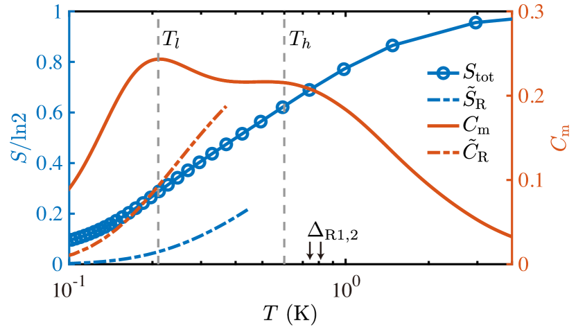
Figure 4: The specific heat $C_{\rm m}$ and total magnetic entropy $S_{\rm tot}$ are shown, which are computed on a YC6$\times$15 cylinder by with tanTRG [72] method with $D=5000$ bond states retained. The higher ($T_{h}\simeq 0.6~{}{\rm K}$) and the lower ($T_{l}\simeq 0.2~{}{\rm K}$) temperature scales are determined from double-peak structure of the specific heat. The roton entropy contributions $\tilde{S}_{\rm R}$ and roton specific heat $\tilde{C}_{R}$ are estimated based on the spectral density of roton modes in Fig. 3(f). Roton gaps $\Delta_{\rm R1}$ and $\Delta_{\rm R2}$ are also indicated in the plot.

Thermodynamics of magnon-roton excitations.— As firstly noticed by Landau [53], rotons are activated at a temperature much lower than the roton gap, and thus contribute significantly to the low-temperature thermodynamics of superfluid helium [64], due to the very large density of states of roton excitations. In Fig. 3(f), we show the $A(\omega)$ obtained by integrating over the momentum $k$, i.e., $A(\omega)=\frac{1}{\mathcal{N}}\sum_{k}A^{zz}(k,\omega)+A^{+-}(k,\omega)$, with $\mathcal{N}$ a normalization factor such that $\int A(\omega)~{}d\omega=1$. A prominent peak of $A(\omega)$ can be observed near the roton mode $\omega\sim\Delta_{\rm R1,R2}$, which may strongly influence the low-temperature properties.

In Fig. 4, we show the calculated entropy $S_{\rm tot}$ and specific heat $C_{\rm m}$ from thermal tensor-network calculations. By taking $A(\omega)$ in the particular energy window as the effective density of states of the roton excitations [51], we also estimate the roton contributions $\tilde{S}_{\rm R}$ and $\tilde{C}_{\rm R}$ at low temperature. From the results in Fig. 4, we find that due to the prominent spectral peak, the roton modes have significant contributions even below $T_{l}\simeq 0.2$ K, despite the considerable roton gap of $\Delta_{\rm R1,R2}\approx 0.78$ K. Therefore, the double magnon-roton excitations with roton dips significantly influence the low-temperature thermodynamics, explaining naturally the giant MCE observed in Na₂BaCo(PO₄)₂ [48].

Discussion and outlook.— In this work, we find a coexistence of three-sublattice spin solidity and gapless Goldstone magnons, and provide spectroscopic evidence for spin supersolidity in NBCP. Predictions have been formulated concerning the emergence of double magnon-roton excitations and the pseudo-Goldstone gap within the spin supersolid phase. To further explore these phenomena, INS measurements with enhanced energy resolution are required.

Beyond NBCP, the main conclusions here on the dynamical properties may also apply to other similarly structured triangular-lattice compounds. Very recently, emerging evidence suggests the presence of a spin supersolid phase within the triangular-lattice cobaltate compound K₂Co(SeO₃)₂, despite of a different extent of easy-axis anisotropy [73, 74]. Owing to the substantial spin exchange interactions present in this triangular-lattice cobaltate, we anticipate that observing the predicted dynamical signatures, including roton modes and pseudo-Goldstone gap, etc, may require less stringent experimental conditions compared to Na₂BaCo(PO₄)₂.

Note added.— In the finalization of the present work, we get aware of two recent studies also on the spin dynamics of spin supersolid phase in Na₂BaCo(PO₄)₂ [75, 76], with main conclusions consistent with our present study.

Supplementary Material for

Spin Supersolid Phase and Double Magnon-Roton Excitations in a Cobalt-based Triangular Lattice

Yuan Gao, et al.

I Data analysis of the neutron scattering measurements

The low energy range with $\omega\in$ [-0.05, 0.05] meV of the INS data in zero field was integrated and treated as the elastic scattering results. As shown in Fig. S1(a), the coexistence of bright magnetic Bragg peaks with the propagation vector of $k$ = (1/3, 1/3, 0.16) and diffusive rod-like scatterings are observed. The latter is along the out-of-plane direction and suggest a quasi two-dimensional nature of NBCP.

The integrated intensities of the magnetic Bragg peaks on top of the diffuse scatterings were extracted for further analysis. As shown in Fig. S1(b), the intensities of the four non-equivalent reflections agree with an UUD configuration of the Co²⁺ moments along the $c$-axis described by the irreducible representation $\Gamma_{1}$. The moment sizes on the $z=0$ layer are estimated to be 0.606(27), $-$0.303(13) and $-$0.303(13) $\mu\rm_{B}$, for the ‘down’, ‘up’, and ‘up’ spins in three sublattices, respectively. The results are well consistent with our previous neutron diffraction results on NBCP also under zero field [48] and supports the presence of out-of-plane spin solidity in the compound.

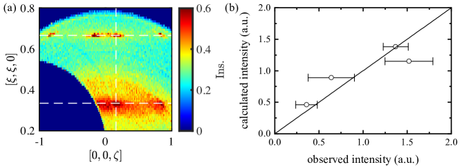
Figure S1: (a) Contour plot of the elastic part of INS results with $\omega\in$ [$-$0.05, 0.05] meV. The data is the same with those in Fig. 1(a) in the main text, but shown in a different color bar to emphasize the rod-like diffuse scatterings. They arise from the almost dispersionless spin excitations at very low energy along the out-of-plane direction. (b) The comparison between the observed and calculated (integrated) intensities of four non-equivalent magnetic reflections for $B=0$ T, adopting the UUD spin configuration of the Co²⁺ moments along the $c$-axis described by the irreducible representation $\Gamma_{1}$.

The low-energy part of the 2.5 T data, with $\omega\in$ [$-$0.1, 0.1] meV, is used for background subtraction for the zero-field INS data. As shown in Fig. S2(c), the spin excitations observed with an in-plane field of $B=2.5~{}{\rm T}$ are clearly gapped. Therefore, we utilize the low-energy part of the 2.5 T data as the intrinsic background to be subtracted for the 0 T case shown in Fig. S2(b), and obtain the result shown in Fig. S2(a). By integrating the scatterings along the out-of-plane [0, 0, $\zeta$] direction, it is found that the spin excitations emanating and away from the ordering vector look quite similar, as shown in Fig. S3(a) for $\zeta\in$ [$-$0.2, 0.2] and Fig. S3(b) for $\zeta\in$ [0.3, 0.7], also indicating clearly a good two dimensionality of NBCP.

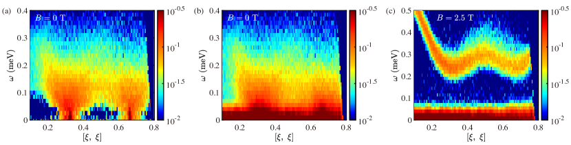
Figure S2: INS results with $B=0$ (a,b) and $B=2.5~{}{\rm T}$ (c). (b) and (c) are the raw data, while (a) is obtained from (b) by subtracting the background below 0.1 meV in (c).

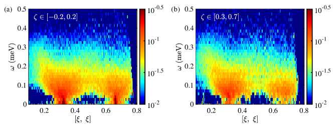
Figure S3: The INS data cut along the high-symmetry $[\xi,\xi]$ direction measured in zero field. Scatterings are integrated along the [$-\eta$, $\eta$, 0] direction for $\eta\in$ [$-$0.4, 0.4], and along the out-of-plane [0, 0, $\zeta$] direction for (a) $\zeta\in$ [$-$0.2, 0.2] and (b) $\zeta\in$ [0.3, 0.7], respectively. The close agreement between the two plots indicates that the compound exhibits robust two-dimensional characteristics.

II Ground State Dynamical Calculations

II.1 Derivation of dynamical spin structure factor and spectral function

In this section, we detail the derivation of ground-state dynamical spin structure factor $S(k,\omega)$ and spectral function $A(k,\omega)$. We start form the real-time correlation function

$$g^{\alpha\beta}(k,t)\equiv\frac{1}{N}e^{{\rm i}E_{0}t}\sum_{i,j}e^{-{{\rm i}k\cdot(r_{i}-r_{j})}}\bra{\psi_{0}}S^{\alpha}_{i}e^{-{\rm i}Ht}S^{\beta}_{j}\ket{\psi_{0}},$$ (S1)

where $\ket{\psi_{0}}$ is the ground state, $E_{0}$ is the ground-state energy, $N$ is the total site number, and $(S_{i}^{\alpha})^{\dagger}=S_{i}^{\beta}$. Then we take the complex conjugate and arrive at

$$g^{\alpha\beta}(k,t)^{*}=\frac{1}{N}e^{-{\rm i}E_{0}t}\sum_{i,j}e^{{-{\rm i}k\cdot(r_{j}-r_{i})}}\bra{\psi_{0}}S^{\alpha}_{j}e^{{\rm i}Ht}S^{\beta}_{i}\ket{\psi_{0}}=g^{\alpha\beta}(k,-t).$$ (S2)

With the real-time correlation function, we obtain the dynamical spin structure factor $S(k,\omega)$

$$\begin{split}S^{\alpha\beta}(k,\omega)&\equiv\int_{-\infty}^{\infty}g^{\alpha\beta}(k,t)e^{{\rm i}\omega t}~{}dt=\int_{0}^{\infty}g^{\alpha\beta}(k,t)e^{{\rm i}\omega t}~{}dt+\int_{0}^{\infty}g^{\alpha\beta}(k,-t)e^{-{\rm i}\omega t}~{}dt\\ &=2\int_{0}^{\infty}{\rm Re}[g^{\alpha\beta}(k,t)e^{{\rm i}\omega t}]~{}dt.\end{split}$$ (S3)

Similar, we can calculate the spectral function $A(k,\omega)\equiv-\frac{1}{\pi}{\rm Im}[G^{\rm R}(k,\omega)]$ where $G^{\rm R}(k,\omega)$ is the retarded Green’s function

$$\begin{split}G^{{\rm R},\alpha\beta}(k,\omega)\equiv&-\frac{\rm i}{N}\sum_{i,j}e^{{-{\rm i}k\cdot(r_{i}-r_{j})}}\int_{0}^{\infty}e^{{\rm i}\omega t}\bra{\psi_{0}}[S^{\alpha}_{i}(t),S^{\beta}_{j}(0)]\ket{\psi_{0}}~{}dt\\ =&-\frac{\rm i}{N}\sum_{i,j}e^{{-{\rm i}k\cdot(r_{i}-r_{j})}}\int_{0}^{\infty}e^{{\rm i}\omega t}(e^{{\rm i}E_{0}t}\bra{\psi_{0}}S^{\alpha}_{i}e^{-{\rm i}Ht}S^{\beta}_{j}\ket{\psi_{0}}-e^{-{\rm i}E_{0}t}\bra{\psi_{0}}S^{\beta}_{j}e^{{\rm i}Ht}S^{\alpha}_{i}\ket{\psi_{0}})~{}dt\\ =&-{\rm i}\int_{0}^{\infty}e^{{\rm i}\omega t}[g^{\alpha\beta}(k,t)-g^{\beta\alpha}(-k,-t)]~{}dt.\end{split}$$ (S4)

Note that the Hamiltonian and the ground state is invariant under the space reversal transformation $r_{i}\rightarrow-r_{i}$, we have $g^{\alpha\beta}(k,t)=g^{\alpha\beta}(-k,t)$. Besides, with zero magnetic field, the Hamiltonian is invariant under the spin flip transformation $S_{i}^{z}\rightarrow-S_{i}^{z},S_{i}^{y}\rightarrow-S_{i}^{y}$, thus we have $g^{+-}(k,t)=g^{-+}(k,t)$. Note that we only consider $A^{+-}(k,\omega),A^{zz}(k,\omega)$ under zero field, we can obtain the spectral function as

$$\begin{split}A^{\alpha\beta}(k,\omega)\equiv&-\frac{1}{\pi}{\rm Im}[G^{{\rm R},\alpha\beta}(k,\omega)]=-\frac{2}{\pi}{\rm Im}[\int_{0}^{\infty}[\cos(\omega t)+{\rm i}\sin(\omega t)]\,{\rm Im}[g^{\alpha\beta}(k,t)]]\\ =&-\frac{2}{\pi}\int_{0}^{\infty}{\rm Im}[g^{\alpha\beta}(k,t)]\sin(\omega t)~{}dt.\end{split}$$ (S5)

In the calculations, we first obtain $\ket{\psi_{0}}$ using density matrix renormalization group [57] and then perform real-time evolution to simulate $\ket{{\psi}^{\prime}(t)}\equiv e^{-{\rm i}Ht}S^{\beta}_{j}\ket{\psi_{0}}$ with time dependent variational principle (TDVP) [58, 59]. Having acquired the real-time correlation function, we proceed to calculate the dynamic structure factor and the spectral functions, which are convolved with an appropriate window function to account for experimental broadening effects, i.e.,

$$\begin{split}S^{\alpha\beta}(k,\omega)&=\int_{0}^{t_{\rm max}}{\rm Re}[g^{\alpha\beta}(k,t)e^{\rm{i}\omega t}]~{}W(\frac{t}{t_{\rm max}})~{}dt,\\ A^{\alpha\beta}(k,\omega)&=-\int_{0}^{t_{\rm max}}{\rm Im}[g^{\alpha\beta}(k,t)]\sin(\omega t)~{}W(\frac{t}{t_{\rm max}})~{}dt,\end{split}$$ (S6)

where $W(t)$ is the Parzen window function, and $t_{\rm max}$ is the maximal TDVP evolution time (in natural unit). The energy resolution $\varepsilon\simeq 8/t_{\rm max}$ as determined by $W(t/t_{\rm max})$, the full width at half maximum (FWHM) of its Fourier transform. In practical calculations, we perform real-time evolution with retained bond dimension up to $D=3000$ on a YC$6\times 15$ lattice for zero field and bond dimension $D=600$ on a YC$6\times 30$ lattice under in-plane field of $B=2.5$ T, with the involved $Y-$type cylindrical lattice shown in Fig. S4 below.

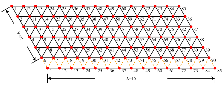
Figure S4: The YC$6\times 15$ lattice employed in the calculations. The number labels the order of the MPS site, and the orange dashed lines represent the periodic boundary condition along $Y$ direction.

II.2 The estimation of energy resolution

The energy resolution $\varepsilon$ is determined by $W(t/t_{\rm max})$, as the FWHM of its Fourier transform. In practice, we choose the Parzen window function following as

$$W(t)=\begin{cases}-2(-1+t)^{3}&\frac{1}{2}<t\leq 1\\ 2(1+t)^{3}&-1\leq t<-\frac{1}{2}\\ 1-6t^{2}-6t^{3}&-\frac{1}{2}\leq t<0\\ 1-6t^{2}+6t^{3}&0\leq t\leq\frac{1}{2}\\ 0&{\rm otherwise}\\ \end{cases},$$ (S7)

As the Fourier transformation reads

$$F[W(t)](\omega)=6\sqrt{\frac{2}{\pi}}\frac{e^{-{\rm i}\omega}(-1+e^{{\rm i}\omega/2})^{4}}{\omega^{4}},$$ (S8)

the energy resolution FWHM can be obtained as $\varepsilon\simeq 8/t_{\rm max}$.

II.3 Estimation of density of states

Here we show the details of density of states (DOS) estimation. We consider the local spectral density $A(\omega)\equiv\frac{1}{N}\sum_{k\in{\rm BZ}}A(k,\omega)$, where BZ is the first Brillouin zone and $N$ is the system size. According to Eq. (S5), we have

$$\begin{split}A^{\alpha\beta}(\omega)\equiv\sum_{k\in{\rm BZ}}A^{\alpha\beta}(k,\omega)=-\frac{2}{\pi}{\rm Im}[\int_{0}^{\infty}e^{{\rm i}\omega t}{\rm Im}[\frac{1}{N}\sum_{k}g^{\alpha\beta}(k,t)]].\end{split}$$ (S9)

Note that

$$\begin{split}\frac{1}{N}\sum_{k}g^{\alpha\beta}(k,t)=&\frac{1}{N}e^{{\rm i}E_{0}t}\sum_{k}\bra{\psi_{0}}S^{\alpha}_{-k}e^{-{\rm i}Ht}S^{\beta}_{k}\ket{\psi_{0}}\\ =&\frac{1}{N}e^{{\rm i}(E_{0}-E_{m})t}\sum_{k,m}||\bra{m}S^{\beta}_{k}\ket{\psi_{0}}||^{2},\end{split}$$ (S10)

where $S^{\beta}_{k}=\frac{1}{\sqrt{N}}\sum_{i}e^{{\rm i}kr_{i}}S_{i}^{\beta}$, $\{\ket{m}\}$ are the eigenstates of $H$ with energy $E_{m}$ and we assume $(S_{-k}^{\alpha})^{\dagger}=S_{k}^{\beta}$. Substitue Eq. (S10) into Eq. (S9), we have

$$\begin{split}A^{\alpha\beta}(\omega)=&-\frac{2}{N\pi}\sum_{k,m}||\bra{m}S^{\beta}_{k}\ket{\psi_{0}}||^{2}\int_{0}^{\infty}{\rm Im}[e^{{\rm i}\omega t}{\rm Im}[e^{{\rm i}(E_{0}-E_{m})t}]]~{}dt\\ =&\frac{1}{N\pi}\sum_{k,m}||\bra{m}S^{\beta}_{k}\ket{\psi_{0}}||^{2}\int_{0}^{\infty}{\rm Re}[e^{{\rm i}(\omega+E_{0}-E_{m})t}]-{\rm Re}[e^{{\rm i}(\omega-E_{0}+E_{m})}]~{}dt\\ =&\frac{1}{N}\sum_{k,m}||\bra{m}S^{\beta}_{k}\ket{\psi_{0}}||^{2}(\delta(\omega+E_{0}-E_{m})-\delta(\omega-E_{0}+E_{m})).\end{split}$$ (S11)

Here we introduce the excitation energy $\varepsilon_{m}\equiv E_{m}-E_{0}$ and only consider the positive energy part, and we can arrive at

$$A^{\alpha\beta}(\omega>0)=\frac{1}{N}\sum_{k,m}||\bra{m}S^{\beta}_{k}\ket{\psi_{0}}||^{2}\,\delta(\omega-\varepsilon_{m}).$$ (S12)

Regarding the low-energy excitation states $\ket{m}$ as free gas of Bogoliubov quasi-particle with energy $\varepsilon_{k}$, the Hamiltonian can be represented as $H\simeq\sum_{k}\varepsilon_{k}\gamma_{k}^{\dagger}\gamma_{k}$. The excitation states can be represented as $\ket{m}\simeq\Pi_{k^{\prime}}\frac{1}{\sqrt{n_{k^{\prime}}!}}(\gamma_{k^{\prime}}^{\dagger})^{n_{k^{\prime}}}\ket{\psi_{0}}$, where $\gamma_{k}$ is the Bogoliubov quasi-particle operator. Therefore, Eq. (S12) can be rewritten as

$$A^{\alpha\beta}(\omega>0)\simeq\frac{1}{N}\sum_{k}||\bra{\psi_{0}}\gamma_{k}S^{\beta}_{k}\ket{\psi_{0}}||^{2}\,\delta(\omega-\varepsilon_{k}),$$ (S13)

where we assume multi-magnon excitation states have vanishing contributions, and $||\bra{\psi_{0}}\gamma_{k}S^{\beta}_{k}\ket{\psi_{0}}||^{2}\sim\mathcal{O}(1)$. With this (crude) approximation, we arrive at

$$A^{\alpha\beta}(\omega>0)\approx\sum_{k}\delta(\omega-\varepsilon_{k}),$$ (S14)

estimates the density of state of magnon excitations with energy $\varepsilon_{k}$. At low temperature, we treat the magnons and rotons as free boson gas, and the entropy and specific heat according to

$$\begin{split}\tilde{S}(T)=&\int_{0}^{\infty}A(\omega)[\frac{\omega/T}{e^{\omega/T}-1}-{\rm ln}(1-e^{-\omega/T})]~{}d\omega,\\ \tilde{C}(T)=&T\frac{\partial\tilde{S}(T)}{\partial T},\end{split}$$ (S15)

where $A(\omega)\equiv A^{+-}(\omega)+A^{zz}(\omega)$ is normalized such that $\int_{0}^{\infty}A(\omega)~{}d\omega=1$.

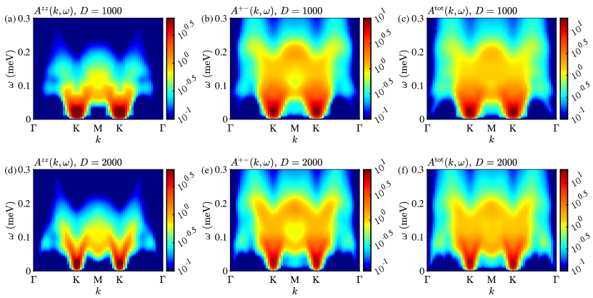
Figure S5: Spectral functions $A^{zz}(k,\omega)$, $A^{+-}(k,\omega)$, and $A^{\rm tot}(k,\omega)=A^{zz}(k,\omega)+A^{+-}(k,\omega)$ computed on a YC$6\times 15$ lattice with different bond dimensions $D=1000,2000$. The energy resolution is set as $\varepsilon\simeq 0.036~{}{\rm meV}$.

II.4 Data convergence

Below we show in Fig. S5 the calculated spectral function results with different bond dimensions retained. By increasing the bond dimension, the magnon-roton excitations become more clear and the downward renormalization at ${\rm M}\equiv[1/2,1/2]$ point becomes more prominent. Besides, we also show the spectral functions with different bond dimensions, momentum points, and energy resolutions. As shown in Fig. S6, we find the spectral functions are well converged with a retained bond dimension $D=3000$.

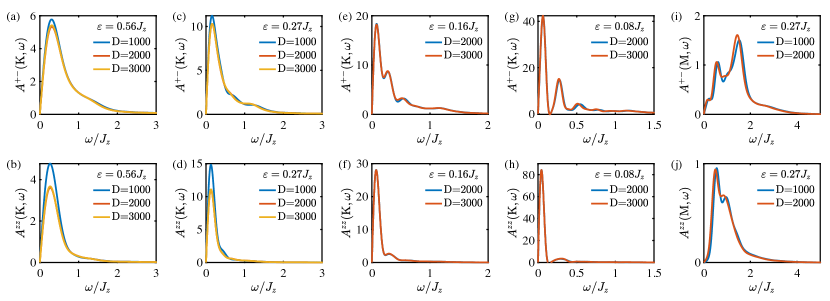
Figure S6: Zero-field spectral functions computed on a YC$6\times 15$ lattice with various bond dimensions $D$, momenta, and spin components.

II.5 High-energy excitation continuum

In this section, we discuss about the high-energy continuum observed in both INS experiments and tensor-network calculations. In Fig. S7(a) we show the experimental results, and in Figs. S7(b-f) spectral functions with different energy resolutions are presented, where the $W$-shape excitation continuum does not sharpen as the energy resolution improves.

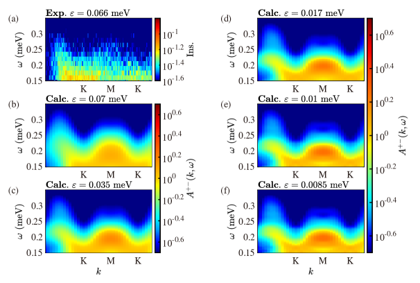
Figure S7: (a) contour plot of INS result. (b-f) spectral function $A^{+-}(k,\omega)$ under different energy resolution with bond dimension $D=1000$.

II.6 Fitting of magnon-maxon-roton excitations

Here we show the magnon-maxon-roton fitting of the calculated spectral function. The terminology magnon, maxon, and roton originates from the excitations spectrum of superfluid helium-4 [77]. Here a magnon represents the gapless linear excitation, also known as the Goldstone mode arising from U(1) symmetry breaking. The maxon corresponds to the quadratic excitation near the peak of the dispersion relation, whereas the roton denotes the quadratic excitation at the bottom of the dispersion curve, characterized by a finite minimum energy. We adopt the undetermined function with the following form

$$f(\xi)=\begin{cases}-k_{0}(\xi-1/3)+\Delta_{0},&\xi\leq 1/3\\ k_{0}(\xi-1/3)+\Delta_{0},&1/3<\xi\leq\xi_{0}\\ -a_{\rm M}(\xi-\xi_{\rm M})^{2}+\Delta_{\rm M},&\xi_{0}<\xi\leq\xi_{1}\\ a_{\rm R}(\xi-1/2)^{2}+\Delta_{\rm R},&\xi_{1}<\xi\\ \end{cases}$$ (S16)

where $\{k_{0},\Delta_{0},\xi_{0},a_{\rm M},\xi_{\rm M},\xi_{1},a_{\rm R},\Delta_{\rm R}\}$ are the fitting parameters. The first two lines are the (pseudo-)Goldstone part, the third line is the maxon part, and the last line is the roton dispersion. Note that $f(\xi)$ should be a continuous function, thus the fitting parameters can be reduced to $\{k_{0},\Delta_{0},\xi_{0},\xi_{\rm M},\xi_{1},\Delta_{\rm R}\}$. With numerical results of the dispersion $\varepsilon_{k}$ obtained from the calculated spectral functions, these parameters can be fitted and the corresponding results are shown in Fig. S8. In examining Goldstone mode excitations determined from $A^{zz}(k,\omega)$, we assume $\Delta_{0}$ to be zero, consistent with the anticipated symmetry breaking scenario. Conversely, when analyzing the $A^{+-}(k,\omega)$ excitation channel, we allow $\Delta_{0}$ to vary, serving as a free parameter to be precisely fitted to the data.

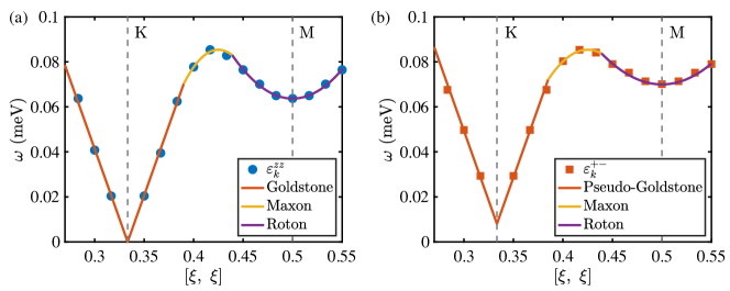
Figure S8: The magnon-maxon-roton fitting of dispersion $\varepsilon_{k}$. Based on the data $\varepsilon_{k}^{zz}$ obtained from the spectral function $A^{zz}$, we arrive at the fitting parameters $\{k_{0}=1.24,\Delta_{0}=0,\xi_{0}=0.39,\xi_{\rm M}=0.439,\xi_{1}=0.425,\Delta_{\rm R}=0.0637\}$. For $\varepsilon_{k}^{+-}$ from the spectral function $A^{+-}$, we find parameters $\{k_{0}=1.24,\Delta_{0}=0.008,\xi_{0}=0.385,\xi_{\rm M}=0.439,\xi_{1}=0.425,\Delta_{\rm R}=0.07\}$. See definitions of these fitting parameters in Eq. (S16).

III Linear spin wave calculations

Details of the linear spin-wave calculations of easy-axis TLAF model $H=\sum_{\langle i,j\rangle}J_{xy}(S_{i}^{x}S_{j}^{x}+S_{i}^{y}S_{j}^{y})+J_{z}S_{i}^{z}S_{j}^{z}$ are shown below, where $\Delta=J_{z}/J_{xy}$. The ground state of the easy-axis TLAF model with $\Delta>1$ is a Y-shaped state in the $x$-$z$ plane. There are three sublattices, namely $A$, $B$, and $C$, and thus three kinds of Holstein-Primakoff bosons, $a$, $b$, and $c$ are introduced. For the sublattice $A$, we have

$$\begin{split}&S^{z}=(S-a^{\dagger}a),\\ &S^{x}=\frac{\sqrt{2S}}{2}(a+a^{\dagger}),\\ &S^{y}=\frac{\sqrt{2S}}{2{\rm i}}(a-a^{\dagger}).\end{split}$$ (S17)

On the other two sublattices, there are angles $\pm\theta$ between spins on A and B(C) sublattices. For sublattice $B$, the transformation reads

$$\begin{split}&S^{z}=\cos\theta~{}(S-b^{\dagger}b)-\sin\theta~{}\frac{\sqrt{2S}}{2}(b+b^{\dagger}),\\ &S^{x}=\sin\theta~{}(S-b^{\dagger}b)+\cos\theta~{}\frac{\sqrt{2S}}{2}(b+b^{\dagger}),\\ &S^{y}=\frac{\sqrt{2S}}{2{\rm i}}(b-b^{\dagger}),\end{split}$$ (S18)

and for sublattice $C$

$$\begin{split}&S^{z}=\cos\theta~{}(S-c^{\dagger}c)+\sin\theta~{}\frac{\sqrt{2S}}{2}(c+c^{\dagger}),\\ &S^{x}=-\sin\theta~{}(S-c^{\dagger}c)+\cos\theta~{}\frac{\sqrt{2S}}{2}(c+c^{\dagger}),\\ &S^{y}=\frac{\sqrt{2S}}{2{\rm i}}(c-c^{\dagger}).\end{split}$$ (S19)

Through the Holstein-Primakoff and Fourier transformations, we arrive at a quadratic form of the Hamiltionian

$$H_{\rm HP}=\sum_{k}\alpha_{k}^{\dagger}H_{0}(k)\alpha_{k},$$

where $\alpha_{k}^{\dagger}=(a_{k}^{\dagger}~{}b_{k}^{\dagger}~{}c_{k}^{\dagger}~{}a_{-k}~{}b_{-k}~{}c_{-k})$ denote the magnon creation operators. The quadratic Hamiltonian is $H_{0}(i,j)=S\,A_{0}(i,j)\,Z(i,j)$, where the $k$-independent symmetric part is $A_{0}=A+A^{\rm T}$, $i,j$ label the matrix index, and $S=1/2$ for the present case. $A$ is a $6\times 6$ upper triangular matrix

$$A=\begin{pmatrix}M&N\\ 0&M\end{pmatrix},$$ (S20)

with

$$M=\begin{pmatrix}-3\Delta\cos\theta&\frac{\cos\theta+1}{2}&\frac{\cos\theta+1}{2}\\ 0&\frac{3}{2}(\sin^{2}\theta-\Delta\cos^{2}\theta-\Delta\cos\theta)&\frac{\cos^{2}\theta+1-\Delta\sin^{2}\theta}{2}\\ 0&0&\frac{3}{2}(\sin^{2}\theta-\Delta\cos^{2}\theta-\Delta\cos\theta)\\ \end{pmatrix},$$ (S21)

and

$$N=\begin{pmatrix}0&\frac{\cos\theta-1}{2}&\frac{\cos\theta-1}{2}\\ \frac{\cos\theta-1}{2}&0&\frac{\cos^{2}\theta-1-\Delta\sin^{2}\theta}{2}\\ \frac{\cos\theta-1}{2}&\frac{\cos^{2}\theta-1-\Delta\sin^{2}\theta}{2}&0\end{pmatrix},$$ (S22)

$\Delta=J_{z}/J_{xy}$ is the anisotropic parameter, and $Z(k)$ is a $6\times 6$ matrix

$$Z(k)=\begin{pmatrix}1&z&z^{*}&1&z&z^{*}\\ z^{*}&1&z&z^{*}&1&z\\ z&z^{*}&1&z&z^{*}&1\\ 1&z&z^{*}&1&z&z^{*}\\ z^{*}&1&z&z^{*}&1&z\\ z&z^{*}&1&z&z^{*}&1\\ \end{pmatrix},$$ (S23)

with $z=\sum_{i}e^{{\rm i}k\delta_{i}}$ with $\delta_{1}=(1,0)$, $\delta_{2}=(-\frac{1}{2},\frac{\sqrt{3}}{2})$, $\delta_{3}=(-\frac{1}{2},-\frac{\sqrt{3}}{2})$. The angle $\theta$ can be obtained by minimizing ground state energy $E_{0}=S^{2}(2\Delta\cos\theta+\Delta\cos^{2}\theta-\sin^{2}\theta)$, and for the realistic parameter $\Delta=1.68$ we have $\theta=128.91^{\circ}$. With this, we diagonalize $H_{HP}$ and obtain the linear spin-wave dispersion shown in Fig. 2 of the main text.