A proof of Vishik’s nonuniqueness Theorem for the forced 2D Euler equation
Abstract.
We give a simpler proof of Vishik’s nonuniqueness Theorem for the forced 2D Euler equation in the vorticity class with . The main simplification is an alternative construction of a smooth and compactly supported unstable vortex, which is split into two steps: Firstly, we construct a piecewise constant unstable vortex, and secondly, we find a regularization through a fixed point argument. This simpler structure of the unstable vortex yields a simplification of the other parts of Vishik’s proof.
1. Introduction
We consider the Euler equation in vorticity form
| (1) |
posed on , for some fixed external force and initial datum
| (2) |
The velocity is recovered from the vorticity through the Biot-Savart law
| (3) |
The aim of this work is to simplify the proof of Vishik’s nonuniqueness Theorem [54, 55]:
Theorem 1.1.
For any there exists a force
| (4) |
where , with the property that there are two different solutions
| (5) |
where , to the Euler equation starting from .
Theorem 1.1 shows sharpness of Yudovich’s uniqueness Theorem for the forced Euler equation. More precisely, Yudovich’s theory implies that if in (4)(5), then necessarily .
In fact, in the construction of Theorem 1.1, both the force and the main solution belong to for positive times. Moreover, for any given , it is not difficult to see that the second solution can be upgraded to be in for positive times. These estimates inevitably deteriorate as . As this information is not relevant in Yudovich’s proof of uniqueness, we have chosen not to include it in the statement of Theorem 1.1.
In a nutshell, Vishik’s proof is split into three steps: (1) Construction of an unstable vortex, which is then shown to be (2) Self-similarly unstable, and (3) Nonlinearly unstable as well.
Step (1) is carried out in [54, 55] by an intricate modification of the power-law vortex . As noticed in [2], by decoupling the parameters governing the self-similar scaling from the decay rate, Vishik’s argument leads to nonuniqueness for the zero initial data , which showcases the primary role played by the forcing .
The observation in [2] that decay does not play a significant role in Vishik’s Theorem suggested us the possibility of obtaining the proof by considering compactly supported vortices. Even more, inspired by simple examples for shear flows (see e.g. [22, Chapter 4]) and vortex patches, we initially aimed to construct a piecewise constant unstable vortex. Remarkably, Step (1) for piecewise constant vortices reduces to an elementary computation. In order to upgrade the piecewise constant vortex to a smooth vortex, we need to apply a fixed point argument in suitable rescaled variables. This step is inspired in [12] but needs of new ideas to be carried out here.
With the new unstable vortex available, the proofs of Steps (2) and (3) from Vishik or [2] would work verbatim. However, since the new vortex is structurally simple, both Steps (2) and (3) admit also several simplifications leading to a straightforward self-contained proof of the entire theorem, which is presented in this work. In any case, the last two steps follow the presentation from book [2] by Albritton, Brué, Colombo, De Lellis, Giri, Janisch, and Kwon, simplifying the arguments whenever possible.
As highlighted in Vishik’s works [54, 55] and the book [2], the rigorous construction of the unstable vortex is a key intermediate step, which is of independent physical and mathematical interest. Indeed, Albritton, Brué and Colombo [1] proved the nonuniqueness of Leray solutions for the forced 3D Navier-Stokes equation by carefully adapting Vishik’s unstable vortex into the cross section of an axisymmetric vortex ring. We remark that, although our vortex differs from Vishik’s one, it fits into the requirements of the paper [1] leading to an alternative example of nonuniqueness for the forced 3D Navier-Stokes equation.
We finally remark that our unstable vortices appear robust enough to be found in more general settings. Indeed, our investigation started because it was not obvious how Vishik’s strategy could be modified to prove nonuniqueness in the more singular (and nonlocal) context of generalized SQG. In this case, the Biot-Savart law (3) is replaced by . The construction and regularization of piecewise constant unstable vortices presented in this paper are however rather flexible and have the potential to work even for all the way up to . Tackling the SQG case () poses even more challenges, notably because is not obtained through a smoothing operator. Both cases, generalized SQG and SQG will be the matter of a forthcoming paper.
1.1. Brief background
The global existence and uniqueness of classical solutions to the 2D Euler equation has been known for almost a century, starting with the works of Wolibner [56] and Hölder [36] in spaces for and . Local well-posedness was previously established by Lichtenstein [43] and Gunther [35]. The global well-posedness in 2D sharply contrasts with the 3D case due to vortex stretching, as demonstrated by Elgindi [23], who showed finite-time singularities with for some in the unforced case. Recently, Córdoba, Martínez-Zoroa and Zheng [18] simplified the proof of this blow-up with a different strategy. Additionally, Córdoba and Martínez-Zoroa [17] upgrade the regularity in the forced case with . We refer to the work [41] by Kiselev and Šverák for the related issue on small scale creation in two dimensions.
In the celebrated paper [57], Yudovich extended the 2D global well-posedness into the vorticity class . The existence of global solutions in for was proved by DiPerna and Majda [21] at the late eighties. Since then, a long-standing open question in the field is whether uniqueness fails for .
In the pioneering works [38, 39], Jia and Šverák introduced, within the context of the 3D Navier-Stokes equation, the idea that nonuniqueness could potentially arise from a self-similar instability. Given that uniqueness is known to be satisfied for small data (in suitable spaces, see e.g. [42]), they conjectured that nonuniqueness could occur due to bifurcations within solutions of the form , for some self-similar steady state. Specifically, they proved in the celebrated paper [38] the existence of self-similar solutions for large data. Later, in [39], the authors speculated that some eigenvalues of the linearization in self-similar coordinates might cross the imaginary axis as increases, leading to the emergence of multiple solutions. While there are numerical evidences, due to Guillod and Šverák [34], supporting the existence of such solutions, the rigorous proof appears to be elusive, primarily because the Jia-Šverák self-similar solutions are not explicit.
In the recent groundbreaking works [54, 55], Vishik was able to construct a self-similarly unstable vortex for the 2D Euler equation, but at the cost of introducing a force. One of the innovative ideas in these works is Vishik’s key observation that, by taking sufficiently large, in order to find a self-similar unstable vortex it suffices to find an unstable vortex in the original Eulerian coordinates. This simplifies the analysis considerably. In the book [2], upon which Sections 5 and 6 of the present work are based, the authors reviewed Vishik’s nonuniqueness Theorem 1.1, providing more details, offering some simplifications and clarifying certain subtle points.
To the best of our knowledge, the question of nonuniqueness without forcing, both for the 2D Euler equation below the Yudovich class and for the 3D Navier-Stokes equation in the Leray class, remains unresolved to date.
In [3, 4] Bressan, Murray, and Shen presented numerical evidences of the nonuniqueness for the unforced 2D Euler equation. Specifically, they introduced two different ways of regularizing a cleverly designed initial vorticity, leading to either one or two algebraic spirals. Recent research on these spirals by García and Gómez-Serrano [30], and by Shao, Wei and Zhang [50], based on the earlier work of Elling [24], could be relevant in the potential proof of nonuniqueness without force.
The first examples of nonuniqueness for weak solutions can be attributed to Scheffer [49] and Shnirelman [51]. Specifically, they constructed weak solutions with compact support in time, to the Euler equation in velocity form. In their seminal work [20], De Lellis and Székelyhidi introduced the convex integration method in hydrodynamics, constructing non-trivial Euler velocities within the energy space for any space dimension . Over the last years, there has been a significant increase in research intensity focused on the method, showcasing its remarkable robustness and flexibility. As a pivotal landmark, this method allowed constructing Euler velocities in exhibiting nonuniqueness [37] by Isett, and dissipating the kinetic energy [7] by Buckmaster, De Lellis, Székelyhidi, and Vicol, thus solving the dissipative part of the 3D Onsager conjecture. See also the work [47] by Novack and Vicol on an intermittent Onsager theorem, based on their joint work [8] with Buckmaster and Masmoudi, as well as the recent work [32] on the -based strong Onsager conjecture by Giri, Kwon and Novack. The conservative part of the Onsager conjecture in any dimension was partially proved by Eyink [27] and later proven in full by Constantin, E, and Titi [15]. See also the work [13] by Cheskidov, Constantin, Friedlander, and Shvydkoy on critical regularity. The dissipative part of the 2D Onsager conjecture was solved recently in [33] by Giri and Radu by means of convex integration. We refer to the recent work [48] by De Rosa and Park for the related issue on anomalous dissipation in two dimensions. In the case with force, Bulut, Huynh and Palasek proved in [10] that the regularity in 3D can be upgraded to . For other applications of convex integration to forced equations, we refer to the recent work [19] by Dai and Friedlander, and the references therein.
As already mentioned in [2], Theorem 1.1 implies that, for any , there exist two different Euler velocities with force starting from . To the best of our knowledge, the problem of nonuniqueness for the unforced Euler equation in the velocity class remains open in the regime .
Unfortunately, it seems not possible with the current convex integration techniques to construct solutions, neither with for , nor with for in two dimensions. Despite this inconvenience, some partial results have been obtained in the last years. In [45] the third author proved the existence, for any , of initial data with for which there are infinitely many admissible solutions . This result shows sharpness of Yudovich’s proof of uniqueness, but with the drawback that the vorticity information is lost for positive times. In [5] Brué and Colombo constructed a Cauchy sequence in the Lorentz space , whose velocities converge to an anomalous weak solution . In [6] Buck and Modena adapted the previous construction for the Hardy space for . This space is also weaker than but, in contrast to , it already embeds into the space of distributions.
Finally, we emphasize that the convex integration method allowed for proving nonuniqueness of Navier-Stokes solutions [9] by Buckmaster and Vicol, and sharpness of the Ladyzhenskaya-Prodi-Serrin criteria [14] by Cheskidov and Luo. Furthermore, the method has been also applied to the construction of non-unique dissipative Euler flows with concrete rough initial data such as vortex sheets [52, 46] by Székelyhidi and the third author, and recently with regularity [25] by Enciso, Peñafiel-Tomás and Peralta-Salas, vortex filaments [29] by Gancedo, Hidalgo-Torné and the third author, and also to the inhomogeneous case [31] by Gebhard, Kolumbán and Székelyhidi. These later developments are inspired by related constructions for IPM [16, 53, 11, 28].
1.2. Organization of the paper
2. Sketch of the proof
In this section we summarize the main ideas for the Proof of Theorem 1.1. The missing technical details will be dealt rigorously in the next sections.
Before going further let us introduce concisely Vishik’s strategy to prove nonuniqueness [54, 55]. Firstly, following the ideas of Jia and Šverák [38, 39], the construction of a self-similar unstable vortex gives hope to find other solutions deviating from as
as , where are two parameters governing the self-similar scaling, and is the unstable eigenvalue (). However, it is not clear how to directly construct a self-similar unstable vortex. Remarkably, Vishik realized and proved that some spectral properties of the linearization in self-similar coordinates can be recovered from the linearization in the original Eulerian coordinates.
Thus, the Proof of Theorem 1.1 divides into three steps: (1) Eulerian, (2) Self-similar, and (3) Nonlinear instability. As discussed in the intro, in our approach, Step (1) is split into two intermediate steps: (1.1) Construction of a piecewise constant unstable vortex, and (1.2) its Regularization.
Step 1. Eulerian instability
We start by recalling how linear stability for the Euler equation leads to the Rayleigh stability equation, which we found convenient to express in vorticity form.
Given a background (steady) vorticity , a perturbation is a second solution to the Euler equation if the deviation satisfies the equation
Here, is the linearization of the Euler equation (1) around . The linearization can be written as
| (6) |
where is a transport operator, is a compact operator, and they are defined by
Here, and are recovered from and respectively through the Biot-Savart law (3).
As usual in Stability theory, as one is lead to study the linear equation
| (7) |
and seek for solutions that grow exponentially in time. That is, for strictly positive,
| (8) |
For solutions of this form, the equation (7) is equivalent to the eigenvalue problem
| (9) |
In other words, instability, at this linear level, translates into the existence of eigenvalues in the right half plane
and eigenfunctions in some suitable Hilbert space, of the linear operator
Remark 2.1.
It is useful to consider the eigenvalue problem (9) for complex-valued vorticities. Since the operator is real, the real-valued solutions to (7) will be recovered by replacing (8) with
| (10) |
Notice that the imaginary part is also a real-valued solution to (7). In particular, if , both the real and imaginary parts of are eigenfunctions. Finally, notice that if is an eigenfunction with eigenvalue , then its complex conjugate is also an eigenfunction with eigenvalue . This remark will become relevant in the Proof of Theorem 1.1.
The caveat of this approach is that the spectral analysis of is quite complicated, even for simple steady states . Thus, we restrict ourselves to the case of radially symmetric ’s called vortices, which in polar coordinates reads as
Next, we choose on which function space the eigenvalue problem will be solved. Given , we seek for eigenfunctions in the subspace of formed by purely -fold symmetric vorticities
| (11) |
Since , we will consider without loss of generality the case .
Definition 2.2.
We say that the vortex is unstable if, for some , there exists satisfying (9) with .
As we will see in Section 3, the space is invariant under the operator . Namely, for ,
where is the angular component of the velocity , and is the Biot-Savart kernel acting on (see (32) and (34) respectively).
Finally, the Rayleigh stability equation is nothing but the eigenvalue problem (9) for
| (12) |
where we have replaced . Observe that translates to . Notice that (12) implies that must vanish wherever . Thus, we can write
in terms of some profile . For that the equation (12) reads as
| (13) |
Thus, Eulerian instability reduces to finding a vortex that admits nontrivial solutions of (13) with . We will show that this is indeed the case and therefore land in our first main result:
Theorem 2.3.
There exists an unstable vortex with zero mean.
As anticipated in the intro, our proof of Theorem 2.3 is split into two steps:
Step 1.1. Piecewise constant unstable vortex
In Section 3 we construct an unstable vortex of the form
in terms of some parameters and , to be determined. Firstly, we choose making the mean of equals zero
This condition guarantees that . Moreover, is Lipschitz and compactly supported with Secondly, since
the equation (13) turns into two conditions for the vector that can be written as a linear system
| (14) |
where the matrix depends on the parameters , and the frequency . Thus, there is an eigenvector if and only if is a root of the characteristic polynomial . Finally, we show in Proposition 3.3 that for any we can choose such that the roots of satisfy .
Step 1.2. Regularization
In Section 4 we prove that there exists a smooth vortex , obtained by suitably regularizing from Step 1.1, which is also unstable for some small . Similarly to Step 1.1, now we need to solve the Rayleigh stability equation (13) in the intervals for . We rescale variables around writing with . Next, we make the asymptotic expansions for eigenfunctions and eigenvalues. Namely, we write
for some profiles , and a constant , to be determined. We also expand
where is another linear operator in . Therefore, the Rayleigh stability equation (13) can be rewritten in the rescaled variables as
Notice that the zero order term vanishes by (14). Since , we want to find satisfying
| (15) |
The first step consists of “inverting” the operator . Unfortunately, since are the eigenvalues of , the kernel and the image of are given by and . We bypass this obstacle by choosing in such a way that the right hand side of (15) becomes “parallel” to . This allows writing (15) in the form
where only depends on the solving (14), while the remainder depends also on . Thus, there is an explicit solution for , and for small enough a fixed point argument in yields a solution as well. Once is fixed, Theorem 2.3 holds by taking
From now on the smooth vortex is fixed and thus we will omit for the sake of simplicity. The use of capital letters will become clear in the following step.
Step 2. Self-similar instability
Let us start by writing the Euler equation in self-similar coordinates
in terms of two parameters to be determined. Notice that the logarithmic time interval is (instead of ). In particular, the physical time corresponds to logarithmic time . It is straightforward to check that given by the change of variables
is a solution to the Euler equation if and only if solves the self-similar Euler equation
| (16) |
where is the linear operator defined by
| (17) |
Notice that (16) agrees with the Euler equation (1) but for the extra term , which vanishes (formally) as . The corresponding velocities and Eulerian forces and are linked by
that is, are recovered from through the Biot-Savart law (3) respectively.
Remark 2.4.
Remark 2.5.
In [2] the parameters are given by and . The reason why we consider this change of variables is purely cosmetic. For instance, it makes more manageable the spectral analysis in the limit .
In the setting of Theorem 1.1, we take the background solution as the time-dependent vortex
| (18) |
where is the unstable vortex from Theorem 2.3, and the corresponding velocity given by the Biot-Savart law (3). Given , we fix the parameter in the regime
to guarantee that the integrability condition (5) is satisfied. Indeed, we have the scaling
| (19) |
The force is defined ad hoc in such a way that (18) becomes a solution. By the radial symmetry of the vortex (and defining the pressure properly) the quadratic term in the Euler equation vanishes, that is, . Thus, the force is defined by
or, equivalently,
Observe that are supported on , and that the integrability condition (4) is also satisfied
| (20) |
Analogously to Step 1, the deviation of a close but different solution to the self similar Euler equation must satisfy
| (21) |
where is the linearization of the self-similar Euler equation (16) around
| (22) |
for defined in (17). The unstable solutions in the limit are governed by exponentially growing solutions to the linearized problem, which we denote by
| (23) |
Hence, we need to understand the corresponding eigenvalue problem
| (24) |
this time for the linear operator .
Definition 2.6.
We say that the vortex is self-similarly unstable if, for some , there exists satisfying (24) with .
An obvious but crucial observation is that
as (or equivalently ), and therefore
| (25) |
The eigenvalue problem (24) for is the self-similar Rayleigh stability equation
| (26) |
in polar coordinates , where we have replaced . Unfortunately, the new term prevents from reproducing Step 1 for . Remarkably, Vishik circumvented this obstacle by showing that the spectrum converges (in a suitable sense) to as . To this end, it is useful to decompose
| (27) |
where
with . Notice that the first term only shifts the spectrum by . As we will explain in Section 5, the transport operator is invertible in . Since is compact, the Operator theory allows to conclude that consists of isolated eigenvalues. Since the dependence on is continuous, there is hope to find an eigenvalue close to . In Section 5 we will review and streamline the proof of the following result from [2]:
Theorem 2.7.
The vortex from Theorem 2.3 is self-similarly unstable for some . Moreover, the corresponding eigenfunction satisfies .
Step 3. Nonlinear instability
The last step for proving Theorem 1.1 requires controlling the nonlinear effects. Coming back to Step 2 (recall (21)-(24)) we decompose the deviation into
where the correcting term must satisfy the equation
| (28) |
coupled with the initial condition
| (29) |
Recall that , while , are the velocities associated to , respectively. If we interpret as a forcing term, since the linear part decays as and the contribution of the quadratic term is expected to be negligible for short times, one can naively expect to gain a slightly faster exponential decay by exploiting the Duhamel formula. In Section 6 we will review this strategy following [2] and provide some simplifications, mainly due to the compact support of our vortex. We will prove the following result:
Proof of Theorem 1.1
We conclude this section by showing how Theorems 2.7 and 2.8 allow proving Theorem 1.1. Coming back to the Eulerian coordinates, Theorems 2.7 and 2.8 imply that the vorticity
satisfies that , because of (19), (25) and (29), and it is a solution to the Euler equation. We just need to show that for different ’s we have different solutions. We recall that
where we have applied the convention that capital letters and stand for self-similar variables. Thus, by applying the scaling
and the reverse triangle inequality, we obtain
If , the right-hand side is positive in a sequence of times as . If , we can assume from the beginning that is real-valued. Otherwise, by Remark 2.1, it would suffice to take its imaginary part instead. This allows concluding that whenever . Finally, we will prove within Section 6.1 that the velocities belong to .
Remark 2.9.
Notice that we have only considered in Theorem 1.1, while there are indeed infinitely many different solutions indexed by . Although these solutions depend on , we have abbreviated to lighten the notation.
Remark 2.10.
In principle, the solutions we have constructed so far blow up in infinite time due to the scaling (20). However, this can be easily solved by taking and vanishing for .
3. Piecewise constant unstable vortex
In this section we prove Theorem 2.3. We start by rigorously deriving the Rayleigh stability equation (13). Firstly, we write the (unforced) Euler equation in polar coordinates
| (31) |
where and are the radial and angular components of the velocity respectively, in the standard basis and .
As we mentioned in Section 2, we restrict to the case of vortices
It is straightforward to see that the corresponding velocity satisfies
namely, , while is equivalent to
| (32) |
The linearization (6) of the Euler equation (31) around reads as
| (33) |
where is recovered from through the Biot-Savart law (3). Notice that only the radial component contributes in (33). In the next lemma we compute for vorticities in the class (11).
Lemma 3.1.
For any and ,
where
| (34) |
Proof.
By writing the Biot-Savart law (3) in polar coordinates (, )
we get
We remark that this is the expression for the real operator (respectively ). Next, we consider acting on complex-valued vorticities. Hence, for , we have
where
| (35) |
The last integral can be computed by means of the Residue Theorem (see Appendix A). ∎
Therefore, the eigenvalue problem can be written as
| (36) |
where . Since must vanish wherever provided that , we can write
and thus the equation (36) reduces to solve
| (37) |
for some profile and eigenvalue with , to be determined.
3.1. Ansatz
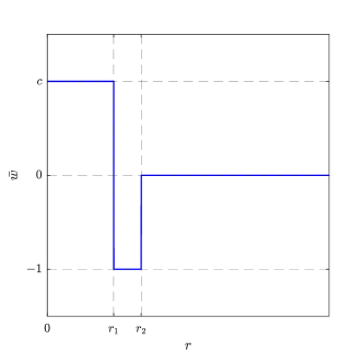
Given some parameters and to be determined, we consider the piecewise constant vorticity profile (see Figure 1)
| (38) |
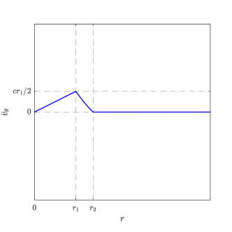
with corresponding (angular) velocity profile (32)
| (39) |
where we have chosen satisfying
| (40) |
In this case we have
Formally, it remains to solve the Rayleigh stability equation (37) at . These are two conditions for the vector that form the linear system
where we split into
| (41) |
Notice that the diagonal matrix comes from the transport operator , and from the compact operator .
In any case, there exists an eigenvector for an eigenvalue if and only if . In the next lemma we compute explicitly this characteristic polynomial of .
Proof.
Proposition 3.3.
For any there exists such that the roots of the characteristic polynomial (42) satisfy . For we can take .
Proof.
The discriminant of the quadratic polynomial (42) equals
Hence, it remains to show that for some . By computing the first two derivatives
and noticing that
we conclude the first statement. For we have . ∎
4. Regularization
Unfortunately, the unstable vortex we constructed in Section 3 is not regular enough: its eigenfunction is a measure concentrated on . In this section we show that there is a regularization that is also an unstable vortex for some small .
We take a standard mollifier with , , and define as usual
By mollifying (instead of ) a few computations are simplified because we get rid of some nonlocal terms. Since we want to regularize the singularities without modifying the vortex outside , we only mollify the indicator functions. To this end, we write the velocity (39) as
where we have abbreviated
Let , to be determined. It is straightforward to check that the profile
| (44) |
is smooth (and agrees with outside by definition). The corresponding vorticity profile is then given by (32)
which is smooth and agrees with outside . Therefore, since
it remains to find an eigenvalue with and a profile satisfying the Rayleigh stability equation (37)
| (45) |
4.1. Rescaling
In this section we zoom into each interval through the change of variables
for and . From now on we will denote
| (46) |
to make the notation more compact.
Lemma 4.1 (Rescaling of the velocity).
It holds
for , where
Proof.
Lemma 4.2 (Rescaling of the vorticity).
It holds
for , where
Proof.
By applying Lemma 4.1, it is straightforward to check that
Then, by computing
we get,
This concludes the proof. ∎
We define in each interval as
where , for some profiles , to be determined. Typically, we will deal with and will speak of to deal with both equations simultaneously and make the notation more compact. Similarly, we define
for some , to be determined. We also make the asymptotic expansion of the kernel
| (47) |
After all this preparation, we can write the Rayleigh stability equation in the rescaled variables.
Lemma 4.3 (Rescaling of the Rayleigh stability equation (45)).
It holds
for . We split the error into
| (48) |
where
4.2. Inverting the linear operator
Notice that we can split into
Observe that when is constant we get back the matrix from (41). We omitted this detail in the introduction for the sake of simplicity. Notice that is a real-valued diagonal operator, and therefore is invertible, and that is constant-valued, that is, . The next lemma takes advantage of this structure to reformulate the Rayleigh stability equation in order to find the corresponding positive eigenvalue.
Lemma 4.4.
The Rayleigh stability equation
is equivalent to
| (51) |
where
| (52) |
and , with
Since is arbitrary, we will take for simplicity.
Proof.
We start by making the change of variables
in terms of some , to be determined. It turns out that must be a constant vector satisfying
| (53) |
Notice that in (53) is acting on constant vectors, and it is therefore given by (41). Since , , and is a basis of , we take
in terms of some , to be determined. Notice that
| (54) |
Hence, multiplying (53) by , we get the compatibility condition for
Notice that since is a basis of . On the other hand, multiplying (53) by , and using (54), we can determine from the following equality
The proof of the lemma is concluded. ∎
4.3. Fixed point argument
For the equation (51) for is explicit and thus we can find a solution . For small we will apply a fixed point argument. It can be shown by a bootstrapping argument that the eigenfunction is indeed smooth. However, since this additional information is not necessary at this point, we omit the proof.
Proposition 4.5.
For every there exists satisfying that: for any there exists solving (51) with . In particular, for .
Proof.
First we check that the linear operators and are bounded in . The operator can be easily bounded by
Similarly, the operator can be bounded by
From the expression (34) and (47) it follows that
Let us denote by the map on the right hand side of (51), that is, we rewrite this equation compactly as
On the one hand, since all the operators involved in are bounded and , there exists such that maps the ball of into itself. On the other hand, given a pair and in , the corresponding pair and given by (52) satisfy
| (55) |
and thus
The boundedness of the operators and and the constant in the statement of the proposition imply that we can choose such that becomes a contraction on . Then, we can apply the classical Banach fixed point theorem to find our required solution. ∎
5. Self-similar instability
In this section we prove Theorem 2.3, and provide growth bounds of the semigroup generated by . We start by decomposing
where is the transport operator
and is the compact operator
Remark 5.1.
As these operators arise from the self-similar Euler equation, we will keep the convention of using uppercase letters for maintaining coherence in notation. It is important to observe that the results applicable to correspond to the (original) Euler equation.
From now on we consider fixed. We define these operators on the subspace of vorticities which has zero mean and are -fold symmetric
| (56) |
By writing the Fourier expansion of in polar coordinates ,
it follows that the -fold symmetry (56) is equivalent to the vanishing of the indices that are not multiples of , and the zero mean condition to
| (57) |
Therefore, we can decompose into the orthogonal direct sum
| (58) |
of the invariant subspaces given in (11), while is given by the condition (57). More precisely, by the Plancherel identity
| (59) |
we consider sums of elements for which (59) is finite. We remark that the operators under consideration are closed and densely defined. In fact, the domain of is , and the domain of and equals
Remark 5.2.
Before embarking on the proof of Theorem 2.7, we recall some classical results in Operator theory. Then, we will analyze and separately, and later . After that, we will compute the growth bound of the semigroup generated by , and provide regularity properties of the eigenfunction.
5.1. Preliminaries
In this section we recall some classical results in Operator theory that will be helpful during the analysis. In general, we will consider a linear operator acting on some Hilbert space , where is the domain of . For a fixed , we will denote and by the space of bounded and compact operators on respectively. In the next sections we will consider .
5.1.1. Spectral theory
The spectrum of is defined as
Let us suppose that is a bounded operator. Then, is called a Fredholm Operator if both the kernel and the cokernel are finite dimensional. In this case, the index of is the integer
We recall a classical result in Spectral theory: the stability of the index of Fredholm operators with respect to compact perturbations (see e.g. [40, Theorem 5.26, Chapter IV]).
Proposition 5.3.
Let be a Fredholm operator and . Then, is a Fredholm operator with .
5.1.2. Semigroup theory
We recall several classical results in Semigroup theory. The first one gives a characterization of strongly continuous semigroups (see e.g. [26, Corollary 3.6, Chapter II]).
Proposition 5.4.
Given and a linear operator , the following are equivalent:
-
(i)
generates a strongly continuous semigroup satisfying for all .
-
(ii)
is closed, densely defined, and for any with , it holds
Next, we recall that, given a strongly continuous semigroup generated by an operator , its growth bound is defined as
| (60) |
The second result from semigroup theory that we need (see e.g. [26, Corollary 2.11, Chapter IV]) relates (60) with the essential bound
where is the quotient space (the so-called Calkin algebra), and the spectral bound
Proposition 5.5.
Given an operator generating a strongly continuous semigroup, it holds
Moreover, is finite for any .
The third result in semigroup theory that we need is the stability of the essential bound with respect to compact perturbations (see e.g. [26, Proposition 2.12, Chapter IV]).
Proposition 5.6.
Given an operator generating a strongly continuous semigroup, and it holds
5.2. The transport operator
Lemma 5.7.
The operator generates a strongly continuous semigroup
where is the flow map
| (61) |
Moreover,
| (62) |
Proof.
Notice that the flow map is defined through a Lipschitz vector field
Hence, the first statement follows from the Cauchy-Lipschitz theory applied to the transport equation. For the second statement, by solving the ODE
we deduce that the Jacobian of the flow map equals
| (63) |
Therefore,
where . ∎
Lemma 5.8.
The resolvent map
| (64) |
is well defined with
| (65) |
For any , the map is continuous.
Proof.
The first statement follows directly from Lemma 5.7 and Proposition 5.4. In fact, a simple integration by parts shows that (64) is the inverse of . Alternatively, (64) is the Laplace transform of the semigroup . For the second statement, given and , the map is continuous since the flow map (61) is defined through a continuous in uniformly Lipschitz vector field. The continuity (indeed analiticity) in is clear from the definition. Hence, (62) allows to apply the dominated convergence theorem in (64). Finally, by applying that is strongly dense and (65), we conclude the proof. ∎
5.3. The compact operator
As pointed in [2], while it is not feasible to extend the Biot-Savart operator throughout , it can be achieved within the subspace , thanks to the following proposition. By a slight abuse of notation, we will continue to denote the Biot-Savart operator as . By combining (66) with the Rellich-Kondrachov Theorem, and the fact that is compactly supported, we deduce the compactness of as a corollary. The second estimate (67) will imply that the velocity of the eigenfunction belongs to .
Lemma 5.9.
There exists such that
| (66) |
for any and , where . If for some , then also
| (67) |
Proof.
Let . Firstly, by applying the -fold symmetry (56), we deduce that
| (68) |
Therefore, by integrating on the ball , we get
from which we deduce that
| (69) |
Therefore, by applying the Poincaré inequality, we get
| (70) |
Secondly, by applying the Plancherel identity on the Biot-Savart law (3), we obtain
These inequalities allow to extend the Biot-Savart operator in by density. For the second statement, since we already have (70) for , it is enough to estimate the -norm of outside . By applying the zero-mean condition of , we get
where we have applied in the first inequality, and the Hölder inequality in the second one. The constant changes from line to line, but it keeps universal. ∎
Corollary 5.10.
The operator is compact.
5.4. The operator
Lemma 5.11.
For any with , the operator is Fredholm with index zero. Therefore, consists of eigenvalues with finite multiplicity.
Proof.
Lemma 5.12.
The operator generates a strongly continuous semigroup.
Proof.
By applying Lemma 5.8 and that is compact, we deduce that the map
| (72) |
is well defined and continuous. In fact, the continuity of (72) in the operator norm follows from combining the fact that the resolvent map (64) is continuous for any fixed , and that can be approximated by finite rank operators. The map allows decomposing (71) into
| (73) |
Let with . By applying (65), we deduce that
and thus the Neumann series
converges in the operator norm. Hence, is invertible with the bound
| (74) |
Finally, by applying again (65), combined with (73) and (74), we deduce that
for any . Then, the claim follows by applying Proposition 5.4. ∎
Lemma 5.13.
The essential bound satisfies
Therefore, is finite for any .
5.5. Proof of Theorem 2.7
Firstly, we claim that there exists satisfying
| (75) |
Since , we know from Theorem 2.3 that (75) holds for . More precisely, there exists an eigenvalue and an eigenfunction . We will prove by contradiction that necessarily (75) is true for some .
Let us suppose that (75) is false. Thus, is invertible for all and . We will first prove that in fact is continuous as a function of .
By applying Lemma 5.13 to , we can take a -oriented circle of radius strictly less than surrounding . By applying Lemma 5.8 coupled with (72) and (73), our hypothesis implies that maps continuously the compact set into
Since the last union forms an open cover, we deduce that there exists such that
uniformly in , and thus, by applying (65) and (73), also
By applying these bounds and the resolvent identity
it follows that the map is continuous from into . As a consequence, the same can be deduce for the map .
Once continuity is obtained, we can consider the Riesz projection
and take limits under the integral sign by the dominated convergence theorem. Therefore, we have
as . However, for any by hypothesis, while , which is a contradiction.
Therefore, there exists for some . By Lemma 5.11, there exists . Since is invariant in each , the functions are also eigenfunctions. Furthermore, since is finite dimensional, is null for all but a finite number of ’s. For , since reads as
necessarily . Therefore, there exists for some .
5.6. Growth bound
In the Proof of Theorem 2.7 we have seen the existence of an eigenvalue . In this section we select the eigenvalue with largest real part, and we compute the growth bound of . In the section about the nonlinear instability we will need the estimate for the growth of the semigroup norm.
Proposition 5.14.
There exists such that . Therefore, for any there exists such that
for all .
5.7. The eigenfunction
In this section we prove that the eigenfunction associated to the eigenvalue appearing in Proposition 5.14 is smooth and compactly supported. Here we see, once again, the advantages of writing the Rayleigh stability equation in vorticity form and dealing with vortices with compact support.
Proposition 5.15.
Let with . Then,
with .
Proof.
The self-similar Rayleigh stability equation (26) can be rewritten as
| (76) |
We remark that (76) is well defined since by construction. On the interval , since and , we deduce that
for some constant . On the interval , since , we deduce that
In this case, since and , necessarily . As a consequence, we have . We have checked that is smooth outside the interval . Let us check that it is smooth inside the interval . Notice that the last integrand in (76) is supported on . Hence, it follows from (76) that . By bootstrapping, the same formula allows to prove that for any . ∎
6. Nonlinear instability
In this section we prove Theorem 2.8. To this end, for any , we consider the unique solution to (28) coupled with the initial condition
| (77) |
The existence and uniqueness of this solution is guaranteed by the Yudovich theory. More precisely, in Eulerian coordinates we have that
is a solution to the Euler equation (1) with the smooth initial condition
| (78) |
where .
Remark 6.1.
On the one hand, recall that and are smooth, compactly supported, and radially symmetric. In particular, . On the other hand, recall that with by Proposition 5.15. In particular, by Lemma 5.9. Since the Euler equation is invariant under rotations and the initial data (78) are -fold symmetric, the uniqueness implies that necessarily (and thus also ) are -fold symmetric as well.
Thus, our task consists in showing that Theorem 2.8 holds for uniformly in . As we will see, the use of the Duhamel formula allows gaining extra exponential decay, but at the cost of having to control the bound under a stronger norm. Following [2], we introduce the subspace of vorticities satisfying
In [2, Proposition 5.0.2] it is proven that satisfies certain properties that allow closing the energy estimates. Due to the compact support of our vortices, some of them can be omitted, namely the control of the decay. In the following proposition we present a simpler version with the minimum necessary bounds, and provide a shorter proof for the sake of completeness.
Proposition 6.2.
There exists such that
for any , where . Moreover, .
Proof.
We start by proving that
| (79) |
Given some fixed , let us denote by the unit ball centered at , and by the average value of in . By applying the Poincaré and Hölder inequalities, we deduce that
where is a constant that changes from line to line, but it is independent of . Hence, by applying the Morrey inequality we get
Since this estimate holds in every ball , we conclude (79). As a corollary, by applying the log-convexity of the -norms, we deduce that
for any . In particular, for this implies that . Therefore, by applying first the Morrey inequality and the Calderon-Zygmund theory, we get
In particular, is continuous. Therefore, letting in (69), we observe that . Consequently, by integrating on the segment with endpoints and we get
For the last statement, we have
| (80) |
It remains to check that is -fold symmetric. By applying (56) and (68), we get
| (81) |
for any . ∎
Since , and the forcing term are smooth and compactly supported for any , it is classical that (and thus also ) enjoy the same properties. Due to (77), given some fixed , we can define to be the largest time such that
| (82) |
for any . Our task is to show that the times satisfying (82) do not diverge to as . If remained positive, we were done. Hence, let us assume from now on that for all sufficiently large. Thus, in particular,
| (83) |
Firstly, we will improve the bound (82) by using the following lemma. Its proof is similar to that of [2, Lemma 5.0.4] and it is the content of our Sections 6.2 and 6.3.
Lemma 6.3.
There exists independent of such that
| (84) |
for all .
6.1. Proof of Theorem 2.8
In this section we show how Lemma 6.3 allows proving Theorem 2.8. Notice that (83) together with (84) implies . Thus, we can take
In Eulerian coordinates, the classical solutions satisfy, for all , the bound
and similarly the corresponding velocities satisfy
By the scaling identities (19), (20) and Remark 6.1, the sequence of vorticities and velocities are uniformly bounded in and , respectively. In this case, it is classical (see e.g. [44, Chapter 10]) that this sequence converges (by taking a subsequence if necessary) to a weak solution of the Euler equation (1). Finally, by applying the sequential weak lower semicontinuity of the -norm, the embedding (recall Proposition 6.2), and (82), we get
for all .
6.2. Baseline estimate
In this section we deal with the part of the -norm for the proof of Lemma 6.3.
Lemma 6.4.
There exists such that
| (85) |
for all .
Proof.
Firstly, recall that satisfies equation (28) with forcing
by Proposition 6.2 and Remark 6.1. Hence, by exploiting the Duhamel formula
together with Proposition 5.14, we estimate, for some fixed and ,
| (86) |
On the one hand, . On the other hand, satisfies the estimate (82). Thus, by applying (80), we obtain the bound
for all . Thus, (86) yields
for all . ∎
6.3. Energy estimates on derivatives
With (85) proven we now proceed to show that
| (87) | ||||
| (88) |
for all . These estimates appear in Lemmas 6.7 and 6.8. Recalling (27), we rewrite (28) as
| (89) |
where we have abbreviated
Throughout the energy estimates, we will need to control the norms appearing in (87)(88) for the terms involving and . These bounds appear in the next two lemmas.
Lemma 6.5.
There exists such that
for all .
Proof.
Lemma 6.6.
There exists such that
| (90) | ||||
| (91) |
for all .
Proof.
We have
We proceed to bound the worst behaved terms. These are the terms involving both and . Recall that (and ) are smooth and supported on a ball of radius . On the one hand, by applying Lemma 5.9 coupled with the baseline estimate (Lemma 6.4), we get
Therefore, we deduce that
and, by additionally applying Proposition 6.2 coupled with (82) and the baseline estimate , we get
The remaining terms are bounded similarly and have the same (or faster) decay. ∎
Notice that until now we have neglected the terms and . In fact, these terms are very problematic since they do not give any extra decay. Following [2], we bypass this problem by estimating the derivatives with respect to the polar coordinates
More precisely, by noticing that
| (92) |
it becomes convenient to perform first energy estimates with respect to the angular derivative. This allows to gain an extra decay on , and then close the energy estimates for .
6.3.1. Estimates on the angular derivative
Lemma 6.7.
There exists such that
| (93) | ||||
| (94) |
for all .
Proof.
For (93), by differentiating (89) with respect to , we get
| (95) |
where we have applied (92)
and also
Multiplying (95) by and integrating by parts yields
where we have applied that and . Thus,
Then, (93) follows by applying Lemmas 6.5 and 6.6 since
for all . For (94), multiplying (95) by yields
| (96) |
where , and we have applied that , and After multiplying (96) by and integrating by parts, we get
Therefore,
| (97) |
Then (94) follows by applying Lemmas 6.5 and 6.6 since
for all . Notice that we need but this is satisfied since Proposition 5.14 guarantees . ∎
6.3.2. Estimates on the radial derivative
Lemma 6.8.
There exists such that
| (98) | ||||
| (99) |
for all .
Proof.
For (98), by differentiating (89) with respect to , we get
| (100) |
where we have applied (92)
and also
After multiplying (100) by we get
| (101) |
where we have applied that , and . Multiplying (101) by and integrating by parts yields
and thus,
For (99), by multiplying (100) by and integrating by parts we get
and thus
Similarly to Lemma 6.7, we conclude the proof by applying Lemmas 6.5 and 6.6, but now coupled with Lemma 6.7. This was the reason for estimating the angular derivative before. ∎
Appendix A Proof of formula (35)
We start by writing
where is the meromorphic function
Hence, by the Residue Theorem we have
We have
It is easy to compute the residue for the simple poles
For the multiple pole we write the Maclaurin series of
where
Hence, for any , we deduce that
By plugging everything together we get (35).
Acknowledgments
The authors thank all participants of the reading seminar on the uniqueness or lack thereof for the Navier-Stokes and Euler equations, which took place in Madrid during the spring of 2023. D.F. and F.M. acknowledge the hospitality and financial support of the Institute for Advanced Study in Princeton during various periods in 2021-2022, as well as the discussions held there with Camillo De Lellis and his group on topics related to Vishik’s construction.
A.C. acknowledges financial support from Grant PID2020-114703GB-I00 funded by MCIN /AEI/ 10.13039/501100011033, Grants RED2022- 134784-T and RED2018-102650-T funded by MCIN/ AEI/ 10.13039/501100011033 and by a 2023 Leonardo Grant for Researchers and Cultural Creators, BBVA Foundation. The BBVA Foundation accepts no responsibility for the opinions, statements, and contents included in the project and/or the results thereof, which are entirely the responsibility of the authors. A.C. and D.F. acknowledge financial support from the Severo Ochoa Programme for Centres of Excellence Grant CEX2019-000904-S funded by MCIN/ AEI/ 10.13039/501100011033. D.F. acknowledges the financial support of QUAMAP and the ERC Advanced Grant 834728. D.F., F.M. and M.S. acknowledge support from PI2021-124-195NB-C32. D.F. and F.M. acknowledge support from CM through the Line of Excellence for University Teaching Staff between CM and UAM. F.M. acknowledges support from the Max Planck Institute for Mathematics in the Sciences. M.S. acknowledges support from PID2022-136589NB-I00 founded by MCIN/AEI/10.13039/501100011033/ and by FEDER (Una manera de hacer Europa) and from “Conselleria d’Innovació, Universitats, Ciència i Societat Digital”: project AICO/2021/223 and programme “Subvenciones para la contratación de personal investigador en fase postdoctoral” (APOSTD 2022), Ref. CIAPOS/2021/28.
References
- [1] D. Albritton, E. Brué, and M. Colombo. Non-uniqueness of Leray solutions of the forced Navier-Stokes equations. Ann. of Math. (2), 196(1):415–455, 2022.
- [2] D. Albritton, E. Brué, M. Colombo, C. De Lellis, V. Giri, M. Janisch, and H. Kwon. Instability and non-uniqueness for the 2D Euler equations, after M. Vishik. Annals of Mathematics Studies. Princeton University Press, Princeton, 2024. In-text citations refer to the arXiv version: arXiv:2112.04943.
- [3] A. Bressan and R. Murray. On self-similar solutions to the incompressible Euler equations. J. Differential Equations, 269(6):5142–5203, 2020.
- [4] A. Bressan and W. Shen. A posteriori error estimates for self-similar solutions to the Euler equations. Discrete Contin. Dyn. Syst., 41(1):113–130, 2021.
- [5] E. Brué and M. Colombo. Nonuniqueness of solutions to the Euler equations with vorticity in a Lorentz space. Comm. Math. Phys., 403(2):1171–1192, 2023.
- [6] M. Buck and S. Modena. Non-uniqueness and energy dissipation for 2D Euler equations with vorticity in Hardy spaces. arXiv:2306.05948, 2023.
- [7] T. Buckmaster, C. De Lellis, L. Székelyhidi, Jr., and V. Vicol. Onsager’s conjecture for admissible weak solutions. Comm. Pure Appl. Math., 72(2):229–274, 2019.
- [8] T. Buckmaster, N. Masmoudi, M. Novack, and V. Vicol. Intermittent convex integration for the 3D Euler equations, volume 217 of Annals of Mathematics Studies. Princeton University Press, Princeton, NJ, [2023] ©2023.
- [9] T. Buckmaster and V. Vicol. Nonuniqueness of weak solutions to the Navier-Stokes equation. Ann. of Math. (2), 189(1):101–144, 2019.
- [10] A. Bulut, M. K. Huynh, and S. Palasek. Convex integration above the Onsager exponent for the forced Euler equations. arXiv:2301.00804, 2023.
- [11] A. Castro, D. Córdoba, and D. Faraco. Mixing solutions for the Muskat problem. Invent. Math., 226(1):251–348, 2021.
- [12] A. Castro and D. Lear. Traveling waves near Couette flow for the 2D Euler equation. Comm. Math. Phys., 400(3):2005–2079, 2023.
- [13] A. Cheskidov, P. Constantin, S. Friedlander, and R. Shvydkoy. Energy conservation and onsager’s conjecture for the euler equations. Nonlinearity, 21(6):1233, 2008.
- [14] A. Cheskidov and X. Luo. Sharp nonuniqueness for the Navier-Stokes equations. Invent. Math., 229(3):987–1054, 2022.
- [15] P. Constantin, W. E, and E. S. Titi. Onsager’s conjecture on the energy conservation for solutions of Euler’s equation. Comm. Math. Phys., 165(1):207–209, 1994.
- [16] D. Cordoba, D. Faraco, and F. Gancedo. Lack of uniqueness for weak solutions of the incompressible porous media equation. Arch. Ration. Mech. Anal., 200(3):725–746, 2011.
- [17] D. Córdoba and L. Martínez-Zoroa. Blow-up for the incompressible 3D-Euler equations with uniform force. arXiv:2309.08495, 2023.
- [18] D. Córdoba, L. Martínez-Zoroa, and F. Zheng. Finite time singularities to the 3D incompressible Euler equations for solutions in . arXiv:2308.12197, 2023.
- [19] M. Dai and S. Friedlander. Non-uniqueness of forced active scalar equations with even drift operators. arXiv:2311.06064, 2023.
- [20] C. De Lellis and L. Székelyhidi, Jr. The Euler equations as a differential inclusion. Ann. of Math. (2), 170(3):1417–1436, 2009.
- [21] R. J. DiPerna and A. J. Majda. Concentrations in regularizations for -D incompressible flow. Comm. Pure Appl. Math., 40(3):301–345, 1987.
- [22] P. G. Drazin and W. H. Reid. Hydrodynamic stability. Cambridge University Press, Cambridge, 2004.
- [23] T. Elgindi. Finite-time singularity formation for solutions to the incompressible Euler equations on . Ann. of Math. (2), 194(3):647–727, 2021.
- [24] V. Elling. Algebraic spiral solutions of the 2d incompressible Euler equations. Bull. Braz. Math. Soc. (N.S.), 47(1):323–334, 2016.
- [25] A. Enciso, J. Peñafiel-Tomás, and D. Peralta-Salas. An extension theorem for weak solutions of the 3d incompressible Euler equations and applications to singular flows. arXiv:2404.08115, 2024.
- [26] K.-J. Engel and R. Nagel. One-parameter semigroups for linear evolution equations, volume 194 of Graduate Texts in Mathematics. Springer-Verlag, New York, 2000. With contributions by S. Brendle, M. Campiti, T. Hahn, G. Metafune, G. Nickel, D. Pallara, C. Perazzoli, A. Rhandi, S. Romanelli and R. Schnaubelt.
- [27] G. L. Eyink. Energy dissipation without viscosity in ideal hydrodynamics. I. Fourier analysis and local energy transfer. Phys. D, 78(3-4):222–240, 1994.
- [28] C. Förster and L. Székelyhidi, Jr. Piecewise constant subsolutions for the Muskat problem. Comm. Math. Phys., 363(3):1051–1080, 2018.
- [29] F. Gancedo, A. Hidalgo-Torné, and F. Mengual. Dissipative Euler flows originating from circular vortex filaments. arXiv:2404.04250, 2024.
- [30] C. García and J. Gómez-Serrano. Self-similar spirals for the generalized surface quasi-geostrophic equations. arXiv:2207.12363, 2022. To appear in J. Eur. Math. Soc.
- [31] B. Gebhard, J. J. Kolumbán, and L. Székelyhidi. A new approach to the Rayleigh-Taylor instability. Arch. Ration. Mech. Anal., 241(3):1243–1280, 2021.
- [32] V. Giri, H. Kwon, and M. Novack. The -based strong Onsager theorem. arXiv:2305.18509, 2023.
- [33] V. Giri and R.-O. Radu. The 2D Onsager conjecture: a Newton-Nash iteration. arXiv:2305.18105, 2023.
- [34] J. Guillod and V. Šverák. Numerical investigations of non-uniqueness for the Navier-Stokes initial value problem in borderline spaces. J. Math. Fluid Mech., 25(3):Paper No. 46, 25, 2023.
- [35] N. Gunther. On the motion of fluid in a moving container. Izvestia Akad. Nauk USSR, Ser. Fiz.-Mat., 20:1323–1348, 1927.
- [36] E. Hölder. Über die unbeschränkte Fortsetzbarkeit einer stetigen ebenen Bewegung in einer unbegrenzten inkompressiblen Flüssigkeit. Math. Z., 37(1):727–738, 1933.
- [37] P. Isett. A proof of Onsager’s conjecture. Ann. of Math. (2), 188(3):871–963, 2018.
- [38] H. Jia and V. Šverák. Local-in-space estimates near initial time for weak solutions of the Navier-Stokes equations and forward self-similar solutions. Invent. Math., 196(1):233–265, 2014.
- [39] H. Jia and V. Šverák. Are the incompressible 3d Navier-Stokes equations locally ill-posed in the natural energy space? J. Funct. Anal., 268(12):3734–3766, 2015.
- [40] T. Kato. Perturbation theory for linear operators. Classics in Mathematics. Springer-Verlag, Berlin, 1995. Reprint of the 1980 edition.
- [41] A. Kiselev and V. Šverák. Small scale creation for solutions of the incompressible two-dimensional Euler equation. Ann. of Math. (2), 180(3):1205–1220, 2014.
- [42] H. Koch and D. Tataru. Well-posedness for the Navier-Stokes equations. Adv. Math., 157(1):22–35, 2001.
- [43] L. Lichtenstein. Über einige Existenzprobleme der Hydrodynamik homogener, unzusammendrückbarer, reibungsloser Flüssigkeiten und die Helmholtzschen Wirbelsätze. Math. Z., 23(1):89–154, 1925.
- [44] A. J. Majda and A. L. Bertozzi. Vorticity and incompressible flow, volume 27 of Cambridge Texts in Applied Mathematics. Cambridge University Press, Cambridge, 2002.
- [45] F. Mengual. Non-uniqueness of admissible solutions for the 2D Euler equation with vortex data. arXiv:2304.09578, 2023.
- [46] F. Mengual and L. Székelyhidi, Jr. Dissipative Euler flows for vortex sheet initial data without distinguished sign. Comm. Pure Appl. Math., 76(1):163–221, 2023.
- [47] M. Novack and V. Vicol. An intermittent Onsager theorem. Invent. Math., 233(1):223–323, 2023.
- [48] L. D. Rosa and J. Park. No anomalous dissipation in two-dimensional incompressible fluids. arXiv:2403.04668, 2024.
- [49] V. Scheffer. An inviscid flow with compact support in space-time. J. Geom. Anal., 3(4):343–401, 1993.
- [50] F. Shao, D. Wei, and Z. Zhang. Self-similar algebraic spiral solution of 2-D incompressible Euler equations. arXiv:2305.05182, 2023.
- [51] A. Shnirelman. On the nonuniqueness of weak solution of the Euler equation. Comm. Pure Appl. Math., 50(12):1261–1286, 1997.
- [52] L. Székelyhidi. Weak solutions to the incompressible Euler equations with vortex sheet initial data. C. R. Math. Acad. Sci. Paris, 349(19-20):1063–1066, 2011.
- [53] L. Székelyhidi, Jr. Relaxation of the incompressible porous media equation. Ann. Sci. Éc. Norm. Supér. (4), 45(3):491–509, 2012.
- [54] M. Vishik. Instability and non-uniqueness in the Cauchy problem for the Euler equations of an ideal incompressible fluid. Part I. arXiv:1805.09426, 2018.
- [55] M. Vishik. Instability and non-uniqueness in the Cauchy problem for the Euler equations of an ideal incompressible fluid. Part II. arXiv:1805.09440, 2018.
- [56] W. Wolibner. Un theorème sur l’existence du mouvement plan d’un fluide parfait, homogène, incompressible, pendant un temps infiniment long. Math. Z., 37(1):698–726, 1933.
- [57] V. Yudovich. Non-stationary flow of an ideal incompressible liquid. USSR Computational Mathematics and Mathematical Physics, 3(6):1407–1456, 1963.
Ángel Castro
Instituto de Ciencias Matemáticas, CSIC-UAM-UC3M-UCM
28049 Madrid, Spain
E-mail address: angel_castro@icmat.es
Daniel Faraco
Departamento de Matemáticas, Universidad Autónoma de Madrid, Instituto de
Ciencias Matemáticas, CSIC-UAM-UC3M-UCM
28049 Madrid, Spain
E-mail address:
daniel.faraco@uam.es
Francisco Mengual
Max Planck Institute for Mathematics in the Sciences
04103 Leipzig, Germany
E-mail address: fmengual@mis.mpg.de
Marcos Solera
Departament d’Anàlisi Matemàtica, Universitat de València
46100 Burjassot, Spain
E-mail address: marcos.solera@uv.es