Seed Selection in the Heterogeneous Moran Process

Abstract

The Moran process is a classic stochastic process that models the rise and takeover of novel traits in network-structured populations. In biological terms, a set of mutants, each with fitness $m\in(0,\infty)$ invade a population of residents with fitness $1$. Each agent reproduces at a rate proportional to its fitness and each offspring replaces a random network neighbor. The process ends when the mutants either fixate (take over the whole population) or go extinct. The fixation probability measures the success of the invasion. To account for environmental heterogeneity, we study a generalization of the Standard process, called the Heterogeneous Moran process. Here, the fitness of each agent is determined both by its type (resident/mutant) and the node it occupies. We study the natural optimization problem of seed selection: given a budget $k$, which $k$ agents should initiate the mutant invasion to maximize the fixation probability? We show that the problem is strongly inapproximable: it is $\operatorname{\mathbf{NP}}$-hard to distinguish between maximum fixation probability 0 and 1. We then focus on mutant-biased networks, where each node exhibits at least as large mutant fitness as resident fitness. We show that the problem remains $\operatorname{\mathbf{NP}}$-hard, but the fixation probability becomes submodular, and thus the optimization problem admits a greedy $(1-\nicefrac{{1}}{{e}})$-approximation. An experimental evaluation of the greedy algorithm along with various heuristics on real-world data sets corroborates our results.

1 Introduction

Modeling and analyzing the spread of a novel trait (e.g., a trend, meme, opinion, genetic mutation) in a population is vital to our understanding of many real-world phenomena. Typically, this modeling involves a network invasion process: nodes represent agents/spatial locations, edges represent communication/interaction between agents, and local stochastic rules define the dynamics of trait spread from an agent to its neighbors.

Network diffusion processes raise several optimization challenges, whereby we control elements of the process to achieve a desirable emergent effect. A well-studied problem is that of influence maximization, which calls to find a seed set of agents initiating a peer-to-peer influence dissemination that maximizes the expected spread thereof; the problem arises in various diffusion models, such as Independent Cascade and Linear Threshold Kempe et al. (2003); Domingos and Richardson (2001); Mossel and Roch (2007); Li et al. (2011), the Voter model Even-Dar and Shapira (2007); Durocher et al. (2022), and geodemographic models of agent mobility Zhang et al. (2020).

Diffusion processes also play a key role in evolutionary dynamics, which model the rules underpinning the sweep of novel genetic mutations in populations and the emergence of new phenotypes in ecological environments Nowak (2006). A classic evolutionary process is the Moran process Moran (1958). In high level, a set of mutants, each with fitness $m\in(0,\infty)$, invade a preexisting population of residents, each with fitness normalized to $1$. Over time, each agent reproduces with rate proportional to its fitness, while the produced offspring replaces a random neighbor. In the long run, the new mutation either fixates in the population (i.e., all agents become mutants) or goes extinct (i.e., all agents remain residents). The probability of fixation is the main quantity of interest, especially under advantageous mutations ($m>1$).

Network structure affects the fixation probability Lieberman et al. (2005); Allen et al. (2017), and may both amplify it Adlam et al. (2015) and suppress it Giakkoupis (2016); Mertzios and Spirakis (2018), while certain structures nearly guarantee mutant fixation Giakkoupis (2016); Goldberg et al. (2019); Pavlogiannis et al. (2018); Tkadlec et al. (2021). The Moran process thus provides a simple stochastic model by which a community of communicating agents reaches consensus; one option has an advantage over another, yet its prevalence (i.e., fixation) depends on the positioning of its initial adherents (i.e., mutants) and on the network structure.

Recent work aims to make the Moran process more realistic by incorporating some form of environmental heterogeneity Maciejewski and Puleo (2014); Brendborg et al. (2022); Melissourgos et al. (2022); Svoboda et al. (2023). Here, the fitness of an agent is not only a function of its type (resident/mutant), but also of its location in space, i.e., the node that it occupies. For example, in a biological setting, the ability to metabolise a certain sugar boosts growth more in environments where such sugar is abundant. Similarly, in a social setting, the spread a trait is more, or less viral depending on the local context (e.g., ads, societal predispositions). Analogous extensions have been recently considered for the Voter evolutionary model Anagnostopoulos et al. (2020); Becchetti et al. (2023); Petsinis et al. (2022).

In this work we generalize the classic Moran process to account for complete environmental heterogeneity, obtaining the Heterogeneous Moran process: for every network node $u$, a mutant (resp., resident) occupying $u$ exhibits fitness $m(u)$ (resp., $r(u)$) specific to that node. We then study the natural optimization problem of seed selection: given a budget $k$, which $k$ nodes should initiate the mutant invasion so as to maximize the fixation probability? Although the seed selection problem has been studied extensively in other diffusion models, this is the first paper to consider it in Moran models. We obtain upper and lower bounds for the complexity of this problem in our Heterogeneous model, which also imply analogous results to other relevant Moran models.

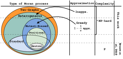
Figure 1: Moran processes (with and without environmental heterogeneity) and the complexity of seed selection.

Contributions. Our main theoretical results are as follows (see Fig. 1 for a summary in the context of Moran models).

1. We prove that computing the fixation probability admits a FPRAS on undirected and unweighted networks that are mutant-biased, where $m(u)\geq r(u)$ for every node $u$.

2. We show that the optimization problem is strongly inapproximable: for any $0<\varepsilon<\nicefrac{{1}}{{2}}$, it is $\operatorname{\mathbf{NP}}$-hard to distinguish between maximum fixation probability $\leq\varepsilon$ and $>1-\varepsilon$.

3. We then focus on mutant-biased networks. We show that the optimization problem remains $\operatorname{\mathbf{NP}}$-hard to solve exactly, but the fixation probability becomes submodular, yielding a greedy $(1-\nicefrac{{1}}{{e}})$-approximation.

Further, we evaluate the greedy algorithm and some standard heuristics for seed selection on real-world data. Our experiments indicate that the greedy algorithm outperforms all heuristics and uncovers high-quality seed sets for varying real-world datasets and problem parameters. Due to space constraints, some proofs appear in the Appendix A.

Technical Challenges. The problem of seed selection was studied recently under the Voter model, which bares some resemblance to the Moran model Durocher et al. (2022). However, the two models are distinct, and results in one do not transfer to the other. Some novel technical challenges we address in this work are as follows.

1. Our NP-hardness and inapproximability proofs are fundamentally different from the NP-hardness of Durocher et al. (2022), and are not limited to weak selection (mutant advantage $\epsilon\rightarrow 0$).

2. Our submodularity proof is based on introducing a novel variant of the Moran process that we call the Loopy process. This also allows us to show that the Heterogeneous Moran process is a special case of the Two-Graph Moran process Melissourgos et al. (2022), thereby extending our hardness results to the latter.

3. Our model accounts for environmental heterogeneity, while the Voter model in Durocher et al. (2022) does not. This complicates our proof for FPRAS.

2 Preliminaries

In this section we introduce the Heterogeneous Moran process and the problem of seed selection.

Population structure. We consider a population of individuals arranged in space. The population structure is represented as a weighted directed graph $G=(V,E,w)$, where each node $u\in V$ represents a single agent, each edge $(u,v)\in E$ represents the fact that $u$ interacts with (influences) $v$, and $w(u,\cdot)$ is a probability distribution capturing the frequency at which $u$ influences $v$. We require that $G$ is strongly connected, i.e., any two nodes are connected by a sequence of edges of non-zero weight. We call $G$ undirected if $E$ is symmetric and $w(u,\cdot)$ is uniform.

Fitness graphs. Trait diffusion in the Heterogeneous Moran process occurs by associating each node with a type: at each moment in time, each node $u$ is either resident or mutant. Moreover, $u$ is associated with a fitness that is type-dependent and represents the rate at which $u$ influences its neighbors while being resident or mutant. We denote the respective fitness values by $r(u)$ and $m(u)$; concretely, these are functions $r,m\colon V\to(0,\infty)$. We call the triplet $\mathcal{G}=(G,(m,r))$ a fitness graph, and denote the minimum and maximum resident and mutant fitnesses in $\mathcal{G}$ as $r_{\min}=\min_{u\in V}r(u)$, and $m_{\max}=\max_{u\in V}m(u)$. We call $\mathcal{G}$ mutant-biased if for all $u\in V$, we have $m(u)\geq r(u)$.

The Heterogeneous Moran process. A configuration is a subset of nodes $X\subseteq V$, representing the mutant nodes in $\mathcal{G}$ at some time point. The fitness of node $u$ in $X$ is defined as

$$f_{X}(u)=\begin{cases}m(u),&\text{if }u\in X\\ r(u),&\text{otherwise}\end{cases}$$

i.e., it is $m(u)$ if $u$ is mutant and $r(u)$ if $u$ is a resident. At time $t=0$ a seed set $S\subseteq V$ specifies the nodes where mutant invasion begins. The Heterogeneous Moran process is a discrete-time stochastic process $\mathcal{X}_{0},\mathcal{X}_{1},\dots,$ of stochastic configurations $\mathcal{X}_{t}\subseteq V$, where $\mathcal{X}_{0}=S$ and for each $t>0$, $\mathcal{X}_{t+1}$ is obtained from $\mathcal{X}_{t}$ by two successive random steps:

1. Birth Event: Pick a node $u$ for reproduction with probability proportional to its fitness, $\frac{f_{X}(u)}{\sum_{v\in V}f_{X}(v)}$.

2. Death Event: Pick a neighbor $v$ of $u$ with probability $w(u,v)$ and make $v$ have the same type as $u$.

Note that the mutant set can both grow and shrink over time.

Fig. 2 illustrates the process on a small example.

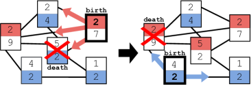
Figure 2: Two steps in the Heterogeneous Moran process; mutants/residents are marked in red/blue; the numbers indicate type-dependent mutant/resident fitness (top/bottom).

Relation to other Moran processes. We recover the Standard Moran process Moran (1958) as a special case of the Heterogeneous process with $r(u)=1$ and $m(u)$ is a constant for all $u\in V$, expressing the mutant fitness. The Neutral Moran process is a further special case of the Standard process, having $\delta=0$ (i.e., residents and mutants have equal fitness). The Positional Moran process Brendborg et al. (2022) is a parameterization of the Standard process by an active set of nodes $\mathcal{A}$, which define the node fitness as $f_{X}(u)=1+\delta$ if $u\in X\cap\mathcal{A}$ and $f_{X}(u)=1$ otherwise. This is also a special case of the Heterogeneous process we study here, with $r(u)=1$ and $m(u)=1+\delta$ if $u\in\mathcal{A}$ and $m(u)=1$ otherwise. The Two-Graphs Moran process Melissourgos et al. (2022) extends the Standard model by accounting for heterogeneity in mobility, as opposed to fitness: mutants and residents propagate via different, type-specific graphs $G_{M}$ and $G_{R}$, respectively, over the same set of nodes but with different edge sets. The Two-Graphs process is more general than our Heterogeneous process; though this connection is not obvious, it is formally implied by an intermediate result we establish in Section 5 towards submodularity.

Fixation probability. In the long run, the process reaches a consensus state $\mathcal{X}_{t}=V$ (mutant fixation) or $\mathcal{X}_{t}=\emptyset$ (mutant extinction). The fixation probability $\operatorname{fp}_{\mathcal{G}}(S)$ is the probability that fixation occurs when the process runs on a fitness graph $\mathcal{G}$ with seed set $S$. The complexity of computing the fixation probability is an open problem, even for the Standard process. In the next section we prove that the fixation probability can be approximated efficiently via Monte Carlo simulations on mutant-biased, undirected fitness graphs.

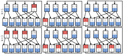
Figure 3: Optimal seed set $S^{*}$ (in red) while varying the mutant fitness and seed size $k$; all residents have fitness 1.

The seed-selection problem. The standard optimization question in invasion processes is optimal seed placement: given a budget $k$, which $k$ nodes $S^{*}$ should initiate the mutant invasion so as to maximize the fixation probability?

$$S^{*}=\operatorname*{arg\,max}_{S\subseteq V,|S|\leq k}\operatorname{fp}_{\mathcal{G}}(S).$$

The optimal seed depends on the graph structure, budget $k$, and node fitnesses. Fig. 3 showcases this intricate relationship, even when all residents have fitness $1$. In particular, the optimal seed $S^{*}$ may contain (i) only nodes with the largest mutant fitness ($k=3$, left), (ii) nodes with both large and small mutant fitness ($k=3$, middle), or (iii) even only nodes with the smallest mutant fitness ($k=3$, right). Moreover, the optimal seed is not monotonic on $k$, i.e., increasing $k$ may yield an optimal seed set that is not a superset of the previous one, and the two may even be disjoint (left, $k=1$ vs $k=3$).

3 Computing the Fixation Probability

Given a seed set $S$ and a fitness graph $\mathcal{G}=(G,(m,r))$, the complexity of computing the fixation probability $\operatorname{fp}_{\mathcal{G}}(S)$ is a long-standing open problem even in the Standard Moran process. This is in sharp contrast to standard cascade models of influence spread, for which the spread function can be approximated efficiently Svitkina and Fleischer (2011).

In the neutral setting ($m(u)=r(u)$ for all $u$), the fixation probability is linear, $\operatorname{fp}_{\mathcal{G}}(S)=\sum_{u\in S}\operatorname{fp}_{\mathcal{G}}(\{u\})$. When the graph is also undirected, $\operatorname{fp}_{\mathcal{G}}(S)=\frac{\sum_{u\in S}\nicefrac{{1}}{{d}}(u)}{\sum_{v\in V}\nicefrac{{1}}{{d}}(v)}$, where $d(x)$ is the degree of $x$ Broom et al. (2010). On the other hand, no closed-form solution is known for the non-neutral setting. However, on undirected graphs the expected time until convergence is polynomial, yielding a fully polynomial-time randomized approximation scheme (FPRAS) via Monte Carlo simulations Díaz et al. (2014); Brendborg et al. (2022). The following lemma generalizes the above result to the Heterogeneous process on mutant-biased graphs. This is in sharp contrast to non-biased graphs, on which the expected time is exponential in general Svoboda et al. (2023).

Lemma 1.

Given an undirected and mutant-biased fitness graph $\mathcal{G}$ and a seed set $S\subseteq V$, the expected time to convergence $T(\mathcal{G},S)$ satisfies $T(\mathcal{G},S)\leq\left(n^{2}\cdot\frac{m_{\max}}{r_{\min}}\right)^{3}$.

Proof.

For a configuration $X$, we define the potential function $\Phi(X)=\sum_{u\in X}\frac{m(u)}{d(u)}$, where $d(u)\geq 1$ is the degree of $u$. Note that $\Phi(X)\leq n\cdot m_{\max}$. We let $\Delta_{t}=\Phi(\mathcal{X}_{t+1})-\Phi(\mathcal{X}_{t})$ be the potential difference in step $t$. In addition, let $\mathcal{X}_{t}=X$, and $R=\{(u,v)\in E\colon u\in X\text{ and }v\not\in X\}$ be the set of edges in $X$ with one endpoint being mutant and the other being resident. Moreover, denote $F=\sum_{u\in V}f_{X}$ as the total population fitness in $X$. Given a pair $(u,v)\in R$, let $p_{u\to v}$ be the probability that $u$ reproduces and replaces $v$. First we show that $\mathbb{E}(\Delta_{t})\geq 0$, i.e., in expectation, the potential function increases in each step:

$$\mathbb{E}(\Delta_{t}) =\sum_{(u,v)\in R}\left(p_{u\to v}\cdot\frac{m(v)}{d(v)}-p_{v\to u}\cdot\frac{m(u)}{d(u)}\right)$$

$$=\sum_{(u,v)\in R}\left(\frac{m(u)}{F}\frac{1}{d(u)}\frac{m(v)}{d(v)}-\frac{r(v)}{F}\frac{1}{d(v)}\frac{m(u)}{d(u)}\right)$$

$$=\sum_{(u,v)\in R}\frac{m(u)(m(v)-r(v))}{{d(u)d(v)}F}\geq 0$$

as $m(v)\geq r(v)$ since $\mathcal{G}$ is mutant-biased. Second, we give a lower bound on the variance of $\Delta_{t}$ when $\emptyset\subset X\subset V$, and thus there exists an edge $(u,v)\in R$. First, we have

$$p_{v\to u}=\frac{r(v)}{F}\frac{1}{d(v)}\geq\frac{r_{\min}}{n\cdot m_{\max}}\frac{1}{n}=\frac{r_{\min}}{n^{2}\cdot m_{\max}}$$

while the potential function changes by $\Delta_{t}\leq-\frac{m(u)}{d(u)}$. Therefore, $\mathbb{P}\left[\Delta_{t}\leq\nicefrac{{-m(u)}}{{d(u)}}\right]\geq\frac{r_{\min}}{n^{2}\cdot m_{\max}}$, and

$$\operatorname{Var}(\Delta_{t}) \geq\mathbb{P}\left[\Delta_{t}\leq-\frac{m(u)}{d(u)}\right]\cdot\left(-\frac{m(u)}{d(u)}-\mathbb{E}(\Delta_{t})\right)^{2}$$

$$\geq\frac{r_{\min}}{n^{2}\cdot m_{\max}}\left(-\frac{m_{\min}}{n}\right)^{2}=\frac{r_{\min}\cdot m_{\min}^{2}}{n^{4}\cdot m_{\max}}.$$

The potential $\Phi$ gives rise to a submartingale with upper bound $B=n\cdot m_{\max}$. The re-scaled function $\Phi(\Phi-2B)+B^{2}$ satisfies the conditions of the upper additive drift theorem Kötzing and Krejca (2019) with initial value at most $B^{2}$ and step-wise drift at least $\operatorname{Var}(\Delta_{t})$. We thus arrive at

$$T(G,S)\leq\frac{B^{2}}{\operatorname{Var}(\Delta_{t})}=\frac{n^{2}\cdot m_{\max}^{2}}{\frac{r_{\min}\cdot m_{\min}^{2}}{n^{4}\cdot m_{\max}}}\leq\frac{n^{6}\cdot m_{\max}^{3}}{r_{\min}^{3}}.\qed$$

Lemma 1 yields an FPRAS for the fixation probability when mutant and resident fitnesses are polynomially (in $n$) related.

Corollary 1.

Given a mutant-biased undirected fitness graph $\mathcal{G}$ with ${m_{\max}}/{r_{\min}}=n^{O(1)}$ and a seed set $S\subseteq V$, the fixation probability $\operatorname{fp}_{\mathcal{G}}(S)$ admits an FPRAS.

4 Hardness of Optimization

Here we turn our attention to the seed selection problem, and prove two hardness results. First, we show that on arbitrary graphs, for any $0<\varepsilon<\nicefrac{{1}}{{2}}$, it is $\operatorname{\mathbf{NP}}$-hard to distinguish between graphs that achieve maximum fixation probability at most $\varepsilon$ and at least $1-\varepsilon$. This is in sharp contrast to standard cascade models of influence spread, for which the optimal spread can be efficiently approximated Kempe et al. (2003). Then we focus on mutant-biased graphs, and show that achieving the maximum fixation probability remains $\operatorname{\mathbf{NP}}$-hard even in this restricted setting.

Our reduction is from the $\operatorname{\mathbf{NP}}$-hard problem Set Cover Karp (1972). Given an instance $(\mathcal{U},\mathcal{S},k)$, where $\mathcal{U}$ is a universe, $\mathcal{S}$ a set of subsets of $\mathcal{U}$, and $k$ a size constraint, the task is to decide whether there exist $k$ subsets in $\mathcal{S}$ that cover $\mathcal{U}$. Wlog, $\mathcal{U}=\bigcup_{A\in\mathcal{S}}A$. We construct a fitness graph $\,\mathcal{G}=(G,(m,r))$ where $G=(V,E,w)$ is a bipartite graph with two parts $V=V_{1}\cup V_{2}$ with $V_{1}=\mathcal{S}$ and $V_{2}=\mathcal{U}$, and define the edge relation as $E=\{(u,v)\in V_{1}\times V_{2}\colon v\in u\}\cup(V_{2}\times V_{1})$ i.e., there is an edge $(u,v)$ for each element $v$ of $\mathcal{U}$ that appears in the set $u$ of $\mathcal{S}$, as well as all possible edges from $V_{2}$ to $V_{1}$. The weight function is uniform: $w(u,v)=1/d(u)$ for each $(u,v)\in E$. The resident fitness is $r(u)=1$ for all $u\in V$. The mutant fitness is parametric on two values $x\geq 1$ and $y\leq 1$ to be fixed later, with $m(u)=x$ if $u\in V_{1}$ and $m(u)=y$ if $u\in V_{2}$. See Fig. 4 for an illustration.

Our construction guarantees upper and lower bounds on the fixation probability depending on whether the seed set forms a set cover of $(\mathcal{U},\mathcal{S})$, as stated in the following lemma.

Lemma 2.

The following assertions hold.

1. If $S$ is not a set cover then $\operatorname{fp}_{\mathcal{G}}(S)\leq 1-\left(\frac{\nicefrac{{1}}{{n}}}{\nicefrac{{1}}{{n}}+(n-1)y}\right)^{n}$.

2. If $S$ is a set cover then

   $$\operatorname{fp}_{\mathcal{G}}(S)\geq\left(\frac{\frac{y}{n^{2}}\left(\frac{\nicefrac{{x}}{{n}}}{\nicefrac{{x}}{{n}}+n}\right)^{n}}{1-\left(1-\frac{y}{n^{2}}\right)\left(\frac{\nicefrac{{x}}{{n}}}{\nicefrac{{x}}{{n}}+n}\right)^{n}}\right)^{n}.$$

Before we prove Lemma 2, we show how Lemma 2 leads to the two hardness results of this section.

Theorem 1.

For any $0<\varepsilon<\nicefrac{{1}}{{2}}$, it is $\operatorname{\mathbf{NP}}$-hard to distinguish between $\max_{S}\operatorname{fp}_{\mathcal{G}}(S)\leq\varepsilon$ and $\max_{S}\operatorname{fp}_{\mathcal{G}}(S)>1-\varepsilon$.

Proof sketch.

We solve the inequalities of Lemma 2, and obtain that there exist $y=1/O(n^{3})$ and $x=O(n^{10})$ satisfying them. As both values are polynomial in $n$, this completes a polynomial reduction from Set Cover to seed selection. ∎

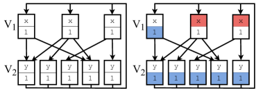
Figure 4: (Left): Graph $G$ for a Set Cover instance with $\mathcal{U}=\{1,2,3,4,5\}$ and $\mathcal{S}=\{\{1,4\},\{1,2,4\},\{3,5\}\}$. (Right): For $k=2$, the optimal seed set forms a Set Cover.

Theorem 2.

In the class of mutant-biased fitness graphs, it is $\operatorname{\mathbf{NP}}$-hard to distinguish between $\max_{S}\operatorname{fp}_{\mathcal{G}}(S)\leq 1-1/(n^{2n})$ and $\max_{S}\operatorname{fp}_{\mathcal{G}}(S)>1-1/(n^{2n})$.

Proof sketch.

We set $y=1$ and solve the second inequality of Lemma 2. We obtain that it is satisfied by some $x=2^{O(n\log n)}$. The fitness graph is mutant-biased as $r(u)=1$ and $m(u)\geq 1$ for all nodes $u$. The description of $x$ is polynomially long in $n$, thus we have a polynomial reduction from Set Cover to seed selection on mutant-biased graphs. ∎

We remark that the class of graphs behind Theorem 2 form a special case of the Positional Moran process Brendborg et al. (2022), by setting as active nodes $\mathcal{A}=V_{1}$ and fitness advantage $\delta=2^{O(n\log n)}$. Thus, the $\operatorname{\mathbf{NP}}$-hardness of Theorem 2 extends to the Positional Moran process.

We now turn our attention to the proof of Lemma 2. By a small abuse of terminology, we say that a configuration $X$ covers $V_{2}$ to denote that the sets in $X\cap V_{1}$ cover $V_{2}$. Item (1) relies on the following intermediate lemma, which intuitively states that, starting from a configuration $X_{1}$ that contains a resident node $v\in V_{2}$ not covered by $X$, the process loses all mutants in $V_{1}$ with large enough probability.

Lemma 3.

From any configuration $X_{1}$ with $V_{2}\setminus(X_{1}\cup\{u\in X_{1}\colon(u,v)\in E\})\neq\emptyset$, the process reaches a configuration $X_{2}$ with $X_{2}\cap V_{1}=\emptyset$ with probability $p\geq\left(\frac{\nicefrac{{1}}{{n}}}{\nicefrac{{1}}{{n}}+(n-1)y}\right)^{|V_{1}|}$.

We can now prove the upper bound of Lemma 2.

Proof Sketch of Lemma 2, Item 1.

First, we show that the probability $q$ of reaching configuration $X_{1}$ such that $V_{2}\setminus(X_{1}\cup\{u\in X_{1}\colon(u,v)\in E\})\neq\emptyset$ is at least $\frac{\nicefrac{{1}}{{n}}}{\nicefrac{{1}}{{n}}+(n-1)y}$. Then, by using Lemma 3 on $X_{1}$ we derive that the process reaches a configuration $X_{2}$ with $X_{2}\cap V_{1}=\emptyset$ with probability at least $\left(\frac{\nicefrac{{1}}{{n}}}{\nicefrac{{1}}{{n}}+(n-1)y}\right)^{|V_{1}|}=q^{|V_{1}|}$. While at configuration $X_{2}$, the process changes configuration when either a resident in $V_{1}$ replaces a mutant in $V_{2}$, or vice versa. Recall that the probability that the first event occurs before the second is at least $q$. Repeating the process for all mutants in $V_{2}\setminus\{v\}$ (as $v$ is already a resident in $X_{2}$) we arrive in a configuration without mutants in $V_{2}$ with probability at least $q^{|V_{2}|-1}$. At this point all mutants have gone extinct, thus $\operatorname{fp}_{\mathcal{G}}(S)\leq 1-q^{1+|V_{1}|+(|V_{2}|-1)}=1-\left(\frac{\nicefrac{{1}}{{n}}}{\nicefrac{{1}}{{n}}+(n-1)y}\right)^{n}.$∎

The following lemma states that, starting from a configuration $X$ that covers $V_{2}$, the process makes all nodes in $V_{2}$ mutants without losing any mutant in $V_{1}$, with certain probability.

Lemma 4.

From any configuration $X$ that covers $V_{2}$, the process reaches a configuration $X^{*}$ with $V_{2}\cup(X\cap V_{1})\subseteq X^{*}$ with probability $p^{*}\geq\left(\frac{\nicefrac{{x}}{{n}}}{\nicefrac{{x}}{{n}}+n}\right)^{|V_{2}|}$.

We can now prove the lower bound of Lemma 2.

Proof Sketch of Lemma 2, Item 2.

We consider $4$ configurations; any configuration $X$ that covers $V_{2}$; $X^{-}$ with less mutants in $V_{1}$ than $X$; $X^{*}$ with same mutants in $V_{1}$ with $X$ and all nodes in $V_{2}$ being mutants; and $X^{+}$ starting from $X^{*}$ includes at least one more mutant in $V_{1}$. The Markov chain in Fig. 5 captures this process where states $S_{1}$, $S_{2}$, $S_{3}$ and $S_{4}$ denote that the process is in configurations $X^{-}$, $X$, $X^{*}$ and $X^{+}$, respectively. To prove the Lemma, we first bound the transition probabilities of Markov chain in Fig. 5. We prove that $p^{+}\geq\frac{\frac{y}{n^{2}}\left(\frac{\nicefrac{{x}}{{n}}}{\nicefrac{{x}}{{n}}+n}\right)^{n}}{1-\left(1-\frac{y}{n^{2}}\right)\left(\frac{\nicefrac{{x}}{{n}}}{\nicefrac{{x}}{{n}}+n}\right)^{n}}$, $p^{*}\geq\Big{(}\frac{\nicefrac{{x}}{{n}}}{\nicefrac{{x}}{{n}}+n}\Big{)}^{n}$ and $q\geq\frac{y}{n^{2}}$. Note that $p^{+}$ is lower-bounded by the probability that a random walk starting in $S_{2}$ (i.e., $X$) gets absorbed in $S_{4}$ (i.e., $X^{+}$). Let $x_{i}$ be the probability that a random walk starting in $S_{i}$ gets absorbed in $S_{4}$. We have $x_{2}=p^{*}\cdot x_{3}+(1-p^{*})\cdot x_{1}$ and $x_{3}=q\cdot x_{4}+(1-q)\cdot x_{2}$, with boundary conditions $x_{1}=0$ and $x_{4}=1$, whence $x_{2}=\frac{q\cdot p^{*}}{1-(1-q)\cdot p^{*}}$. Since $X\!\subset\!X^{+}$, the set $X^{+}$ also covers $V_{2}$, thus the reasoning repeats for up to $n$ steps until fixation, resulting in $\operatorname{fp}_{\mathcal{G}}(X)\geq(p^{+})^{n}$. ∎

Figure 5: The Markov chain for the process of Lemma 4.

5 Monotonicity and Submodularity

Theorem 1 rules out polynomial-time algorithms for any non-trivial answer to seed selection. For mutant-biased graphs, Theorem 2 states that the problem remains $\operatorname{\mathbf{NP}}$-hard to solve exactly, but does not rule out tractable approximations. Indeed, here we prove that, on mutant-biased graphs, the fixation probability is monotone and submodular, thus seed selection admits a constant-factor approximation. Our proofs are based on coupling arguments. Instead of applying these arguments directly to the Heterogeneous Moran process, we introduce a slight variation, the Loopy process, and argue that it is equivalent to the Heterogeneous process in the sense that it preserves the fixation probability.

The Loopy process. Our Loopy variant is similar to the original process, but we slightly modify the underlying fitness graph $\mathcal{G}=(G,(m,r))$ in each step based on the current configuration $X$. Without loss of generality, we let every node $u\in V$ have a self-loop $(u,u)\in E$ (we can always assign $w(u,u)=0$). When the original process is at some configuration $X$, different nodes reproduce at different rates. When the Loopy process is at configuration $X$, we construct a fitness graph $\mathcal{G}_{X}=(G_{X},(\mathbf{1},\mathbf{1}))$, where $\mathbf{1}$ is the constant function $u\mapsto 1$, and $G_{X}=(V,E,w_{X})$ is a graph with the same structure as $G$, but the weight function is modified by adjusting the self-loop probability of each node, as follows.

$$w_{X}(u,v)=\begin{cases}\frac{f_{X}(u)}{m_{\max}}\cdot w(u,v),&\text{ if }u\neq v\\ 1-\frac{f_{X}(u)}{m_{\max}}(1-w(u,v)),&\text{ if }u=v\end{cases}$$

Intuitively, all nodes in $\mathcal{G}_{X}$ reproduce at equal rates as they have the same fitness regardless of their type. The new weight function $w_{X}$ compensates for this uniformity of reproduction rates: nodes that formerly had lower fitness now have stronger self-loops, which restores the relative propagation rates between neighbors. That is, the probability distribution $\mathbb{P}[\mathcal{X}_{t+1}|\mathcal{X}_{t+1}\neq\mathcal{X}_{t}]$, and thus the fixation probability, is identical in the two processes, as stated in the following lemma.

Lemma 5.

For any seed set, the Heterogeneous and Loopy Moran processes share the same fixation probability.

Relation to the Two-Graphs process. The Loopy process is a special case of the recent Two-Graphs Moran process Melissourgos et al. (2022). To obtain the Two-Graphs process, we define two graphs $G_{M}$ and $G_{R}$ for mutants and residents, respectively. For each edge $(u,v)$, its weight $w_{M}(u,v)$ in $G_{M}$ and $w_{R}(u,v)$ in $G_{R}$, is obtained from Section 5, considering that $u\in X$ and $u\not\in X$, respectively. In turn, Lemma 5 implies that the hardness of Theorems 1 and 2 also hold for seed selection in the Two-Graphs model.

Monotonicity. The following monotonicity corollary follows from Lemma 5 and the monotonicity of the Two Graphs process (Melissourgos et al., 2022, Corollary 6).

Corollary 2.

For any fitness graph $\mathcal{G}=(G,(m,r))$ and any two seed sets $S\subseteq S^{\prime}$, we have $\operatorname{fp}_{\mathcal{G}}(S)\leq\operatorname{fp}_{\mathcal{G}}(S^{\prime})$.

Submodularity. We now turn our attention to the submodularity of the fixation probability in the Heterogeneous Moran process. Although the function is not submodular in general, we prove that it becomes submodular on mutant-biased fitness graphs. In particular, we show that for any two seed sets $S,T\subseteq V$, the following submodularity condition holds:

$$\operatorname{fp}_{\mathcal{G}}(S)+\operatorname{fp}_{\mathcal{G}}(T)\geq\operatorname{fp}_{\mathcal{G}}(S\cup T)+\operatorname{fp}_{\mathcal{G}}(S\cap T)$$

Our proof is via a four-way coupling of the corresponding processes starting in one of the seed sets of Section 5.

Lemma 6.

For any mutant-biased fitness graph $\,\mathcal{G}=(G,(m,r))$, the fixation probability $\operatorname{fp}_{\mathcal{G}}(S)$ is submodular.

Proof.

Let $\mathcal{M}_{1}=(\mathcal{X}^{1}_{t})_{t\geq 0}$, $\mathcal{M}_{2}=(\mathcal{X}^{2}_{t})_{t\geq 0}$, $\mathcal{M}_{3}=(\mathcal{X}^{3}_{t})_{t\geq 0}$, and $\mathcal{M}_{4}=(\mathcal{X}^{4}_{t})_{t\geq 0}$, be four Loopy processes with seed sets $S$, $T$, $S\cup T$ and $S\cap T$, respectively. To prove submodularity, we employ two tricks for $\mathcal{M}_{3}$. First, along its configurations $\mathcal{X}^{3}_{t}$, we also keep track of the set of mutants $\mathcal{Y}_{t}$ (resp., $\mathcal{Z}_{t}$) that are copies of some initial node in $S$ (resp., $T$). Whenever a node $v$ receives the mutant trait from a neighbor $u$, we place $v$ in $\mathcal{Y}_{t+1}$ (resp., $\mathcal{Z}_{t+1}$) following the membership of $u$ in $\mathcal{Y}_{t}$ (resp., $\mathcal{Z}_{t}$). Initially, $\mathcal{Y}_{0}=S$ and $\mathcal{Z}_{0}=T$. Second, with probability 1, every run of $\mathcal{M}_{3}$ that results in fixation, eventually (i.e., if we let the process run on) leads to the fixation of $S$ or $T$ (possibly both, assuming $S\cap T\neq\emptyset$); that is, every node is a copy of some node in $S$ or $T$. We thus compute the fixation probability with seed $S\cup T$ by summing over runs in which $S$ or $T$ fixates.

To prove submodularity, we consider this refined view of the process and establish a four-way coupling between $\mathcal{M}_{1}$, $\mathcal{M}_{2}$, $\mathcal{M}_{3}$ and $\mathcal{M}_{4}$ that guarantees the following invariants: (i) $\mathcal{X}^{1}_{t}\cup\mathcal{X}^{2}_{t}\subseteq\mathcal{X}^{3}_{t}$, (ii) $\mathcal{X}^{4}_{t}\subseteq\mathcal{X}^{1}_{t}\cap\mathcal{X}^{2}_{t}$, (iii) $\mathcal{Y}_{t}\subseteq\mathcal{X}^{1}_{t}$, and (iv) $\mathcal{Z}_{t}\subseteq\mathcal{X}^{2}_{t}$. Now, consider any execution in which $\mathcal{M}_{3}$ fixates. Since $S$ or $T$ eventually fixates in $\mathcal{M}_{3}$, due to invariants (iii) and (iv), at least one of $\mathcal{M}_{1},\mathcal{M}_{2}$ fixates as well. Moreover, if $\mathcal{M}_{4}$ also fixates, due to invariant (ii), both $\mathcal{M}_{1}$ and $\mathcal{M}_{2}$ fixate. Thus the invariants guarantee submodularity.

The invariants hold at $t=0$. Now, consider some arbitrary time $t$ with the four processes at configurations $\mathcal{X}^{j}_{t}=X^{j}$, for $j\in\{1,2,3,4\}$, $\mathcal{Y}_{t}=Y$, and $\mathcal{Z}_{t}=Z$. To obtain $\mathcal{X}^{j}_{t+1}$, we sample the same node $u$ for reproduction with probability $\nicefrac{{1}}{{n}}$ in all processes. From invariants (i) and (ii), and since $m(u)\geq r(u)$, we derive that $w_{X_{3}}(u,u)\leq w_{X_{j}}(u,u)\leq w_{X_{4}}(u,u)$ for $j\in\{1,2\}$, as residents have a larger self-loop weight. In $\mathcal{M}_{3}$, we choose a neighbor $v$ of $u$ with probability $w_{X_{3}}(u,v)$ and propagate the trait of $u$ to $v$. In $\mathcal{M}_{1}$, $\mathcal{M}_{2}$ and $\mathcal{M}_{4}$, if $u=v$, we perform the same update; otherwise, if $u$ has the same type as in $\mathcal{M}_{3}$, we also perform the same update. From the invariants, if $u$ is resident in $\mathcal{M}_{3}$ then the same holds in all other processes, while if $u$ is a mutant in $\mathcal{M}_{3}$ then the same holds in at least one of $\mathcal{M}_{1}$, $\mathcal{M}_{2}$ (depending on whether $u\in Y$ and $u\in Z$), and if that holds for $\mathcal{M}_{1}$ and $\mathcal{M}_{2}$, then it holds for $\mathcal{M}_{4}$. However, if $u$ is resident in $\mathcal{M}_{j}$ for some $j\in\{1,2\}$ but mutant in $\mathcal{M}_{3}$, i.e., $u\in X^{3}\setminus X^{j}$, then, due to invariant (ii), $u$ is also resident in $\mathcal{M}_{4}$, i.e., $u\in X^{3}\setminus X^{4}$; then, in $\mathcal{M}_{j}$ and $\mathcal{M}_{4}$, $u$ propagates to itself with probability $w_{X_{j}}(u,u)-w_{X_{3}}(u,u)\geq 0$, and to $v$ with the remaining probability $1-(w_{X_{j}}(u,u)-w_{X_{3}}(u,u))$. It follows that all three invariants are maintained. ∎

Following Nemhauser et al. (1978), monotonicity and submodularit lead to the following approximation guarantee.

Theorem 3.

Given a mutant-biased fitness graph $\mathcal{G}$ and budget $k$, let $S^{*}$ be an optimal seed set and $S_{\text{gr}}$ the solution of the Greedy algorithm. We have $\operatorname{fp}_{\,\mathcal{G}}(S_{\text{gr}})\geq\left(1-\nicefrac{{1}}{{e}}\right)\operatorname{fp}_{\,\mathcal{G}}(S^{*})$.

The Greedy algorithm builds the seed set iteratively by choosing the node that yields the maximum fixation probability gain. Finally, note that due to symmetry, on resident-biased fitness graphs ($m(u)\leq r(u)$ for all $u$), $\operatorname{fp}_{\mathcal{G}}(S)$ is supermodular, thus Greedy offers no approximation guarantees.

Figure 6: Fixation probability vs. $k$.

Figure 7: Fixation probability vs. $m_{\max}$.

6 Experimental Analysis

Here, we present our experimental evaluation of the Greedy algorithm and other network heuristics, varying the seed size $k$ and the maximum mutant fitness $m_{\max}$.

Name	$|V|$	$|E|$	Directed	Edge-Weighted
Facebook	324	5028	✗	✗
Colocation	242	53188	✗	✓
Mammalia	327	1045	✓	✓
Polblogs	793	15839	✓	✗

Table 1: Dataset characteristics.

Datasets. We use four real-world networks from Netzschleuder, SNAP and Network Repository (Table 1).

1. Facebook: A Facebook ego network in which nodes represent profiles and edges indicate friendship.

2. Colocation: A proximity network of students and teachers of a French school. Edge weights count the frequency of contact between individuals during a two-day period.

3. Mammalia: An animal-contact network based on movements of voles (Microtus agrestis). Each edge weight counts the common traps the two voles were caught in.

4. Polblogs: A network of hyperlinks among a large set of U.S. political weblogs from before the 2004 election.

Our experiments are not meant to be exhaustive, but rather indicative of the performance of the greedy algorithm and common network-optimization heuristics on a few diverse networks. We set the resident fitness to $1$, while the mutant fitness of each node $u$ is determined by sampling a uniform distribution $m(u)\sim\mathcal{U}(1,m_{\max})$. This results in mutant-biased graphs, for which Theorem 3 guarantees that the fixation probability admits a Monte Carlo approximation.

Greedy and Baselines. We evaluate the performance of the standard Greedy algorithm behind Theorem 3 Nemhauser et al. (1978) against four common baseline algorithms from related literature on seed selection under diffusion processes Brendborg et al. (2022); Zhao et al. (2021); Liu et al. (2017).

1. Random: select uniformly at random.

2. Degree: select by smallest degree.

3. Closeness: select by smallest closeness centrality.

4. PageRank: select by smallest PageRank score.

The Random selection strategy is a standard baseline to measure the intricacy of the problem. Degree is the only existing algorithm for seed selection in the Moran model, and is optimal for undirected and unweighted networks under the neutral setting (but underperforms when $m_{\max}>1$). On the other hand, Closeness and PageRank take into account the structure of the graph and its connectivity. For these two centrality heuristics we also tried selecting the top-$k$-nodes by largest value, which resulted in worse performance. All Monte Carlo simulations were run over $5000$ iterations.

Performance vs. $\bm{k}$. Fig. 6 shows performance as the size constraint $k$ increases for a fixed mutant fitness distribution. In agreement with Corollaries 2 and 6, the performance of all algorithms rises as $k$ grows, while Greedy has diminishing returns. Notably, Greedy outperforms all heuristics especially for small size constraints, while Pagerank forms high quality solutions for the undirected and unweighted graph Facebook. On the other hand, seed selection becomes more challenging for directed (Mammalia, Polblogs) and edge-weighted graphs (Colocation, Mammalia), in which only Greedy uncovers high-quality seed sets.

Performance vs. $\bm{m}$. Fig. 7 shows performance as the mutant fitness interval $[1,m_{\max}]$ increases, for fixed size $k$. Random selection performs poorly, showing that the problem is not trivial, while the other two heuristics have mixed performance. On the other hand, Greedy achieves a steady, high-quality performance in all datasets and problem parameters.

7 Conclusion

We studied a natural optimization problem pertaining to network diffusion by the Heterogeneous Moran process, namely selecting a set of seed nodes that maximize the effect of the invasion. To our knowledge, this is the first paper to study this standard optimization problem on Moran models. We showed that the problem is strongly inapproximable in general, but becomes approximable on mutant-biased graphs, although the exact solution remains $\operatorname{\mathbf{NP}}$-hard. Several interesting questions remain open for future work, such as, is seed selection hard in the Standard model; and are there tighter approximations for mutant-biased graphs?

Appendix A Appendix

First we prove Lemma 3 and Lemma 4, that are used in the analysis of Lemma 2.

See 3

Proof.

Let $q=\frac{\nicefrac{{1}}{{n}}}{\nicefrac{{1}}{{n}}+(n-1)y}$. While at $X_{1}$, there exists at least one resident node $v\in V_{2}$ that is not covered by any mutant in $V_{1}$. Let $X^{\prime}_{1}$ be the first configuration that the process reaches in which the number of mutants in $V_{1}$ has changed from $X_{1}$ (i.e., $V_{1}$ either has one more, or one less mutant in $X^{\prime}_{1}$ compared to $X_{1}$). Let $F=\sum_{u\in V}f_{X_{1}}(u)$ be the total population fitness at $X_{1}$. The probability that $v$ replaces a mutant in $V_{1}$ in a single step is $p_{1}\geq\frac{1}{F}\frac{1}{n}$. On the other hand, the probability that any mutant in $V_{2}$ replaces a resident in $V_{1}$ in a single step is $p_{2}\leq\frac{|V_{2}|y}{F}\leq\frac{(n-1)y}{F}$. Thus, the probability that $V_{1}$ has lost a mutant in $X^{\prime}_{1}$ is at least $\frac{p_{1}}{p_{1}+p_{2}}\geq\frac{\nicefrac{{1}}{{n}}}{\nicefrac{{1}}{{n}}+(n-1)y}=q$.

Now, observe that $X^{\prime}_{1}$ satisfies the conditions of $X_{1}$, i.e., $V_{2}\setminus(X^{\prime}_{1}\cup\{u\in X^{\prime}_{1}\colon(u,v)\in E\})\neq\emptyset$. Thus we can repeat the above process until all nodes in $V_{1}$ have become residents, leading to the desired configuration $X_{2}$ with probability

$$p\geq q^{|V_{1}|}=\left(\frac{\nicefrac{{1}}{{n}}}{\nicefrac{{1}}{{n}}+(n-1)y}\right)^{|V_{1}|}\qed$$

See 4

Proof.

Let $q=\frac{x/n}{x/n+n}$, and let $F=\sum_{u\in V}f_{X}(u)$ be the total population fitness in $X$. As long as there are residents in $V_{2}$, the probability that a mutant node in $V_{1}$ replaces a resident in $V_{2}$ is at least $p_{1}\geq\frac{x}{F}\frac{1}{n}$. On the other hand, the probability that a resident in $V_{2}$ (resp. $V_{1}$) replaces a mutant in $V_{1}$ (resp. $V_{2}$) is at most $p_{2}\leq\frac{|V_{2}|}{F}$ (resp. $p_{3}\leq\frac{|V_{1}|}{F}$). The probability that the first event occurs before the second and third one is thus at least $\frac{p_{1}}{p_{1}+p_{2}+p_{3}}\geq\frac{x/n}{x/n+|V_{2}|+|V_{1}|}=\frac{x/n}{x/n+n}=q$. Observe that any other event that changes the configuration (i.e., mutants in $V_{2}$ replacing residents in $V_{1}$) results in a configuration that also covers $V_{2}$, thus we can repeat the above argument until all nodes in $V_{2}$ become mutants, which occurs with probability at least

$$p^{*}\geq q^{|V_{2}|}\geq\left(\frac{\nicefrac{{x}}{{n}}}{\nicefrac{{x}}{{n}}+n}\right)^{|V_{2}|}\qed$$

We continue with proving the upper and lower bounds of Lemma 2. See 2

Proof.

We prove the two assertions separately.

1. Item 1: First, we argue that with probability at least $q=\frac{\nicefrac{{1}}{{n}}}{\nicefrac{{1}}{{n}}+(n-1)y}$, the process reaches a configuration $X_{1}$ such that $V_{2}\setminus(X_{1}\cup\{u\in X_{1}\colon(u,v)\in E\})\neq\emptyset$. Indeed, since $S$ does not form a set cover, there exists a node $v\in V_{2}$ that has no mutant incoming neighbor in $V_{1}$. If $v\not\in S$, we are done. Otherwise, the probability that, in a single step, $v$ is replaced by any resident neighbor in $V_{1}$ is at least $p_{1}\geq\frac{1}{F}\frac{1}{n}$, where $F=\sum_{u\in V}f_{S}(u)$ is the total population fitness at $S$. On the other hand, any resident in $V_{1}$ is replaced by mutants in $V_{2}$ with probability $p_{2}\leq\frac{|V_{2}|y}{F}\leq\frac{(n-1)y}{F}$. Thus, the probability that the process reaches a desired configuration $X_{1}$ is at least $\frac{p_{1}}{p_{1}+p_{2}}\geq\frac{1/n}{1/n+(n-1)y}=q$.

   Second, Lemma 3 applies on $X_{1}$ to show that the process reaches a configuration $X_{2}$ with $X_{2}\cap V_{1}=\emptyset$ with probability at least $\left(\frac{\nicefrac{{1}}{{n}}}{\nicefrac{{1}}{{n}}+(n-1)y}\right)^{|V_{1}|}=q^{|V_{1}|}$.

   Third, while at configuration $X_{2}$, the process changes configuration when either a resident in $V_{1}$ replaces a mutant in $V_{2}$, or vice versa. We have already argued in the first step that the probability that the first event occurs before the second is at least $q$. Now, we repeat this process until all mutants in $V_{2}$ have become residents, which occurs with probability at least $q^{|V_{2}|-1}$, as $v\in V_{2}$ is already a resident in $X_{2}$. At this point the mutants have gone extinct, thus $\operatorname{fp}_{\mathcal{G}}(S)\leq 1-q^{1+|V_{1}|+(|V_{2}|-1)}=1-\left(\frac{\nicefrac{{1}}{{n}}}{\nicefrac{{1}}{{n}}+(n-1)y}\right)^{n}.$

2. Item 2: We first prove the following statement. Consider the process at any configuration $X$ that covers $V_{2}$, and let $p^{+}$ be the probability that it reaches a subsequent configuration $X^{+}$ with at least one more mutant in $V_{1}$. We will show that $p^{+}\geq\frac{\frac{y}{n^{2}}\left(\frac{\nicefrac{{x}}{{n}}}{\nicefrac{{x}}{{n}}+n}\right)^{n}}{1-\left(1-\frac{y}{n^{2}}\right)\left(\frac{\nicefrac{{x}}{{n}}}{\nicefrac{{x}}{{n}}+n}\right)^{n}}$. Given any such configuration $X$, let $p^{*}$ be the probability that the process reaches a subsequent configuration $X^{*}$ with $V_{2}\cup(X\cap V_{1})\subseteq X^{*}$. By Lemma 4, we have $p^{*}\geq\Big{(}\frac{\nicefrac{{x}}{{n}}}{\nicefrac{{x}}{{n}}+n}\Big{)}^{|V_{2}|}\geq\Big{(}\frac{\nicefrac{{x}}{{n}}}{\nicefrac{{x}}{{n}}+n}\Big{)}^{n}$. While at $X^{*}$, the process only progresses when a mutant in $V_{2}$ replaces a resident in $V_{1}$, or a resident in $V_{1}$ replaces a mutant in $V_{2}$. As long as there are residents in $V_{1}$, the probability $q$ that a mutant from $V_{2}$ replaces a resident in $V_{1}$ before any such resident reproduces satisfies $q\geq\frac{\frac{y}{F}\frac{1}{n}}{\frac{y}{F}\frac{1}{n}+\frac{|V_{1}|}{F}}\geq\frac{\frac{y}{F}\frac{1}{n}}{\frac{y}{F}\frac{1}{n}+\frac{n-1}{F}}=\frac{y}{y+(n-1)n}\geq\frac{y}{n^{2}}$, where the last inequality holds as $y\leq 1\leq n$. If this happens, we reach the desired configuration $X^{+}$. Otherwise, a resident in $V_{1}$ replaces a mutant in $V_{2}$, the resulting configuration still covers $V_{2}$, and the argument repeats. The Markov chain in Fig. 5 captures this process. The states $S_{2}$, $S_{3}$ and $S_{4}$ denote that the process is in configurations $X$, $X^{*}$ and $X^{+}$, respectively. Hence, $p^{+}$ is lower-bounded by the probability that a random walk starting in $S_{2}$ (i.e., $X$) gets absorbed in $S_{4}$ (i.e., $X^{+}$). Let $x_{i}$ be the probability that a random walk starting in $S_{i}$ gets absorbed in $S_{4}$. We have $x_{2}=p^{*}\cdot x_{3}+(1-p^{*})\cdot x_{1}$ and $x_{3}=q\cdot x_{4}+(1-q)\cdot x_{2}$, with boundary conditions $x_{1}=0$ and $x_{4}=1$, whence $x_{2}=\frac{q\cdot p^{*}}{1-(1-q)\cdot p^{*}}$. Since $X\!\subset\!X^{+}$, set $X^{+}$ also covers $V_{2}$, thus the reasoning applies for up to $n$ steps until fixation, resulting in $\operatorname{fp}_{\mathcal{G}}(X)\geq(p^{+})^{n}\geq\left(\frac{\frac{y}{n^{2}}\Big{(}\frac{\nicefrac{{x}}{{n}}}{\nicefrac{{x}}{{n}}+n}\Big{)}^{n}}{1-\Big{(}1-\frac{y}{n^{2}}\Big{)}\Big{(}\frac{\nicefrac{{x}}{{n}}}{\nicefrac{{x}}{{n}}+n}\Big{)}^{n}}\right)^{n}.$∎

We continue with the proof of Theorem 1 and Theorem 2. To make our analysis easier, we first prove two simple lemmas.

Lemma 7.

For every $\zeta>0$, we have $\ln\left(1+\frac{1}{\zeta}\right)\geq\frac{1}{\zeta+1}$.

Proof.

$$\left(1+\frac{1}{\zeta}\right)^{\zeta+1}\geq e$$

$$\Leftrightarrow \ln\left(1+\frac{1}{\zeta}\right)^{\zeta+1}\geq\ln e$$

$$\Leftrightarrow \ln\left(1+\frac{1}{\zeta}\right)\geq\frac{1}{\zeta+1}\qed$$

Lemma 8.

Let $p\in(0,1)$, and $\beta\leq\frac{\ln(\nicefrac{{1}}{{p}})}{n}$. We have

$$\left(\frac{1}{1+\beta}\right)^{n}\geq p$$

Proof.

Let $\gamma=1+\nicefrac{{1}}{{\beta}}$, thus $\beta=\nicefrac{{1}}{{(\gamma-1)}}$. Then

$$\gamma=1+\frac{1}{\beta}\geq 1+\frac{n}{\ln\left(\frac{1}{p}\right)}$$

Moreover

$$\frac{1}{1+\beta}=\frac{1}{1+\frac{1}{\gamma-1}}=\frac{1}{\frac{\gamma}{\gamma-1}}=\frac{\gamma-1}{\gamma}=1-\frac{1}{\gamma}$$

Let $k=\ln(\nicefrac{{1}}{{p}})^{-1}$, thus $p=e^{-\nicefrac{{1}}{{k}}}$ and $\gamma\geq nk+1$. We have

$$\left(1-\frac{1}{nk+1}\right)^{nk}\geq e^{-1}$$

$$\Rightarrow \left(1-\frac{1}{nk+1}\right)^{n}\geq e^{-\frac{1}{k}}$$

$$\Rightarrow \left(1-\frac{1}{\gamma}\right)^{n}\geq p$$

$$\Rightarrow \left(\frac{1}{1+\beta}\right)^{n}\geq p$$

as desired. ∎

See 1

Proof.

The proof is by algebraic manipulation on the inequalities of Lemma 2. In particular, we argue that there exist $x$ and $y$ that have polynomially-long description (in $n$) for which the inequalities stated in the theorem hold. In turn, this completes a polynomial reduction from Set Cover to distinguishing between $\max_{S}\operatorname{fp}_{\mathcal{G}}(S)\leq\varepsilon$ and $\max_{S}\operatorname{fp}_{\mathcal{G}}(S)>1-\varepsilon$ in the Heterogeneous Moran process.

First, assume that $S$ does not form a set cover, thus Item (1) of Lemma 2 applies. We solve the corresponding inequality to arrive at a suitable value for $y$. In particular, for $\operatorname{fp}_{\mathcal{G}}(S)\leq\varepsilon$, it suffices to find a $y$ small enough such that

$$~{}1-\left(\frac{\frac{1}{n}}{\frac{1}{n}+(n-1)y}\right)^{n}\leq\varepsilon$$

$$\Leftrightarrow ~{}1-\varepsilon\leq\left(\frac{1}{1+n(n-1)y}\right)^{n}$$ (3)

Using Lemma 8 for $p=1-\varepsilon$, we set

$$~{}n(n-1)y=\beta\leq\frac{\ln\left(\frac{1}{p}\right)}{n}$$

$$\Rightarrow ~{}y\leq\frac{1}{O(n^{3})}$$

as $\varepsilon$ is fixed. Hence $y$ suffices to be polynomially small in $n$ for the inequality of Item (1) of Lemma 2 to hold.

On the other hand, if $S$ forms a set cover, Item (2) of Lemma 2 applies. We solve the corresponding inequality to arrive at a suitable value for $x$. In particular, for $\operatorname{fp}_{\mathcal{G}}(S)>1-\varepsilon$, it suffices to find an $x$ large enough such that

$$~{}\left(\frac{\frac{y}{n^{2}}\left(\frac{\frac{x}{n}}{\frac{x}{n}+n}\right)^{n}}{1-\left(1-\frac{y}{n^{2}}\right)\left(\frac{\frac{x}{n}}{\frac{x}{n}+n}\right)^{n}}\right)^{n}>1-\varepsilon$$

Substituting with $\alpha=\left(\frac{x}{x+n^{2}}\right)^{n}$, we have

$$~{}\left(\frac{\frac{y}{n^{2}}\alpha}{1-\left(1-\frac{y}{n^{2}}\right)\alpha}\right)^{n}>1-\varepsilon$$

$$\Rightarrow ~{}\left(\frac{\frac{y}{n^{2}}\alpha}{1-\alpha+\frac{y}{n^{2}}\alpha}\right)^{n}>1-\varepsilon$$

$$\Rightarrow ~{}\left(\frac{1}{1+\frac{n^{2}(1-\alpha)}{y\alpha}}\right)^{n}>1-\varepsilon$$

Using Lemma 8 for $p=1-\varepsilon$, we set

$$~{}\frac{n^{2}(1-\alpha)}{y\alpha}=\beta\leq\frac{\ln\left(\frac{1}{p}\right)}{n}$$

$$\Rightarrow ~{}\alpha\geq\frac{n^{3}}{n^{3}+yc}$$

where $c=\ln(\nicefrac{{1}}{{p}})$ is a constant. We thus have

$$\left(\frac{x}{x+n^{2}}\right)^{n}\geq\frac{n^{3}}{n^{3}+yc}$$

$$\Rightarrow ~{}\left(\frac{1}{1+\frac{n^{2}}{x}}\right)^{n}\geq\frac{n^{3}}{n^{3}+yc}$$

Using Lemma 8 for $p=\frac{n^{3}}{n^{3}+yc}$, we set

$$~{}\frac{n^{2}}{x}=\beta\leq\frac{\ln\left(\frac{1}{q}\right)}{n}$$

$$\Rightarrow ~{}x\geq\frac{n^{3}}{\ln\left(\frac{1}{q}\right)}=\frac{n^{3}}{\ln\left(1+\frac{1}{\frac{n^{3}}{cy}}\right)}$$

Using Lemma 7 for $\zeta=\frac{n^{3}}{cy}=O(n^{6})$ as $c=O(1)$ and $y=1/O(n^{3})$, we have

$$x\geq\frac{n^{3}}{\frac{1}{n^{7}}}=O(n^{10})$$

Thus $x$ suffices to be polynomially large in $n$ for the inequality of Item (2) of Lemma 2 to hold. ∎

See 2

Proof.

The proof is by algebraic manipulation on the inequalities of Lemma 2 for the specific case where $y=1$ and $x\geq y$. Observe that this makes the corresponding graph mutant-biased. In particular, we argue that there exists an $x$ with a polynomially-long description (in $n$) for which the inequalities stated in the theorem hold. In turn, this completes a polynomial reduction from Set Cover to distinguishing between $\max_{S}\operatorname{fp}_{\mathcal{G}}(S)\leq 1-1/(n^{2n})$ and $\max_{S}\operatorname{fp}_{\mathcal{G}}(S)>1-1/(n^{2n})$ in the Heterogeneous Moran process.

First, assume that $S$ does not form a set cover. Item (1) of Lemma 2 for $y=1$ gives

$$\operatorname{fp}_{\mathcal{G}}(S)\leq 1-\left(\frac{1}{1+(n-1)n}\right)^{n}\leq 1-\frac{1}{n^{2n}}$$

On the other hand, if $S$ forms a set cover, Item (2) of Lemma 2 applies. For $y=1$, we solve the corresponding inequality to arrive at a suitable value for $x$. In particular, for $\operatorname{fp}_{\mathcal{G}}(S)>1-\frac{1}{n^{2n}}$, it suffices to find an $x$ large enough such that

$$\operatorname{fp}_{\mathcal{G}}(S)\geq\left(\frac{\frac{1}{n^{2}}\left(\frac{\frac{x}{n}}{\frac{x}{n}+n}\right)^{n}}{1-\left(1-\frac{1}{n^{2}}\right)\left(\frac{\frac{x}{n}}{\frac{x}{n}+n}\right)^{n}}\right)^{n}>1-\frac{1}{n^{2n}}$$

Substituting with $a=\left(\frac{x}{x+n^{2}}\right)^{n}$, we have

$$~{}\left(\frac{\frac{1}{n^{2}}\alpha}{1-\left(1-\frac{1}{n^{2}}\right)\alpha}\right)^{n}>1-\frac{1}{n^{2n}}$$

$$\Rightarrow ~{}\left(\frac{\frac{1}{n^{2}}\alpha}{1-\alpha+\frac{1}{n^{2}}\alpha}\right)^{n}>1-\frac{1}{n^{2n}}$$

$$\Rightarrow ~{}\left(\frac{1}{1+\frac{n^{2}(1-\alpha)}{\alpha}}\right)^{n}>1-\frac{1}{n^{2n}}$$

Using Lemma 8 for $p=1-\frac{1}{n^{2n}}$, we set

$$~{}\frac{n^{2}(1-\alpha)}{\alpha}=\beta\leq\frac{\ln\left(\frac{1}{p}\right)}{n}$$

$$\Rightarrow ~{}\alpha\geq\frac{n^{3}}{n^{3}+c}$$

where $c=\ln(\nicefrac{{1}}{{p}})$. We thus have

$$\left(\frac{x}{x+n^{2}}\right)^{n}\geq\frac{n^{3}}{n^{3}+c}$$

$$\Rightarrow ~{}\left(\frac{1}{1+\frac{n^{2}}{x}}\right)^{n}\geq\frac{n^{3}}{n^{3}+c}$$

Using Lemma 8 for $p=\frac{n^{3}}{n^{3}+c}$, we set

$$~{}\frac{n^{2}}{x}=\beta\leq\frac{\ln\left(\frac{1}{q}\right)}{n}$$

$$\Rightarrow ~{}x\geq\frac{n^{3}}{\ln\left(\frac{1}{q}\right)}=\frac{n^{3}}{\ln\left(1+\frac{1}{\frac{n^{3}}{c}}\right)}$$

Using Lemma 7 for $\zeta=\frac{n^{3}}{c}$, we have

$$x\geq\frac{n^{3}}{\frac{1}{\frac{n^{4}}{c}}}=\frac{n^{7}}{c}$$

Finally, recall that $c=\ln(\nicefrac{{1}}{{p}})=\ln\left(1+\frac{1}{n^{2n}-1}\right)$. Using Lemma 7 again with $\beta=n^{2n}-1$, we conclude that

$$x\geq\frac{n^{7}}{\ln\left(1+\frac{1}{n^{2n}-1}\right)}\geq\frac{n^{7}}{\frac{1}{n^{2n}}}=2^{O(n\log n)}$$

Observe that $x$ has polynomially-long (in $n$) description, thus our reduction from Set Cover is in polynomial time. ∎

See 5

Proof.

Consider the Heterogeneous and Positional Moran process, and assume that they are in the same configuration $Z\subseteq V$. Consider any edge $(u,v)\in E$ with $u\neq v$. Let $p_{u\rightarrow v}$ and $p^{\prime}_{u\rightarrow v}$ be the probabilities of $u$ transferring its trait to $v$ under the Heterogeneous and Loopy Moran processes, respectively, when in configuration $Z$. By the definition of the models, we have

$$p_{u\rightarrow v}=\frac{f_{Z}(u)}{{F}}w(u,v),\,\,\,p^{\prime}_{u\rightarrow v}=\frac{1}{n}w_{Z}(u,v)=\frac{f_{Z}(u)\cdot w(u,v)}{n\cdot m_{\max}}.$$

Moreover, let $R=E\setminus\{(x,x)\colon x\in V\}$ be the set of edges without the self loops in $G$. Note that, form $Z$, each process can progress to a distinct configuration $Z^{\prime}\neq Z$ only if a node $u$ transfers its trait along an edge $(u,v)\in R$. Let $p_{1}$ and $p^{\prime}_{1}$ be the probability that this occurs in the Heterogeneous and Loopy process, repsectively, and we have

$$p_{1}=\sum\limits_{(x,y)\in R}\frac{f_{Z}(x)}{F}w(x,y),\,\,\,\,\,\,\,\,\,p_{1}^{\prime}= \sum\limits_{(x,y)\in R}\frac{1}{n}w_{Z}(x,y)$$

$$= \sum\limits_{(x,y)\in R}\frac{f_{Z}(x)\cdot w(x,y)}{n\cdot m_{\max}}.$$

Finally, observe that

$$\frac{p_{u\rightarrow v}}{p_{1}}=\frac{\frac{f_{Z}(u)}{{F}}w(u,v)}{\sum\limits_{(l,r)\in R}\frac{f_{Z}(l)}{F}w(l,r)}=\frac{{f_{Z}(u)}w(u,v)}{\sum\limits_{(l,r)\in R}{f_{Z}(l)}w(l,r)}$$

$$\frac{p^{\prime}_{u\rightarrow v}}{p^{\prime}_{1}}=\frac{\frac{f_{Z}(u)\cdot w(u,v)}{n\cdot m_{\max}}}{\sum\limits_{(l,r)\in R}\frac{f_{Z}(l)\cdot w(l,r)}{n\cdot m_{\max}}}=\frac{{f_{Z}(u)}w(u,v)}{\sum\limits_{(l,r)\in R}{f_{Z}(l)}w(l,r)}.$$

Thus, the probability distribution $\mathbb{P}[\mathcal{X}_{t+1}=X|\mathcal{X}_{t+1}\neq\mathcal{X}_{t}]$ is the same in the two processes, yielding the same fixation probability starting from the same seed set, as desired. ∎

References

- Adlam et al. [2015] Ben Adlam, Krishnendu Chatterjee, and Martin A Nowak. Amplifiers of selection. Proceedings of the Royal Society A: Mathematical, Physical and Engineering Sciences, 471(2181):20150114, 2015.
- Allen et al. [2017] Benjamin Allen, Gabor Lippner, Yu-Ting Chen, Babak Fotouhi, Naghmeh Momeni, Shing-Tung Yau, and Martin A Nowak. Evolutionary dynamics on any population structure. Nature, 544(7649):227–230, 2017.
- Anagnostopoulos et al. [2020] Aris Anagnostopoulos, Luca Becchetti, Emilio Cruciani, Francesco Pasquale, and Sara Rizzo. Biased opinion dynamics: When the devil is in the details. In Christian Bessiere, editor, Proceedings of the Twenty-Ninth International Joint Conference on Artificial Intelligence, IJCAI-20, pages 53–59. International Joint Conferences on Artificial Intelligence Organization, 7 2020. Main track.
- Becchetti et al. [2023] Luca Becchetti, Vincenzo Bonifaci, Emilio Cruciani, and Francesco Pasquale. On a voter model with context-dependent opinion adoption. In Edith Elkind, editor, Proceedings of the Thirty-Second International Joint Conference on Artificial Intelligence, IJCAI-23, pages 38–45. International Joint Conferences on Artificial Intelligence Organization, 8 2023. Main Track.
- Brendborg et al. [2022] Joachim Brendborg, Panagiotis Karras, Andreas Pavlogiannis, Asger Ullersted Rasmussen, and Josef Tkadlec. Fixation maximization in the positional moran process. In Proceedings of the AAAI Conference on Artificial Intelligence, volume 36, pages 9304–9312, 2022.
- Broom et al. [2010] M Broom, C Hadjichrysanthou, J Rychtář, and BT Stadler. Two results on evolutionary processes on general non-directed graphs. Proc. Royal Soc. A, 466(2121), 2010.
- Díaz et al. [2014] Josep Díaz, Leslie Ann Goldberg, George B Mertzios, David Richerby, Maria Serna, and Paul G Spirakis. Approximating fixation probabilities in the generalized moran process. Algorithmica, 69(1):78–91, 2014.
- Domingos and Richardson [2001] Pedro Domingos and Matt Richardson. Mining the network value of customers. In Proceedings of the seventh ACM SIGKDD international conference on Knowledge discovery and data mining, pages 57–66, 2001.
- Durocher et al. [2022] Loke Durocher, Panagiotis Karras, Andreas Pavlogiannis, and Josef Tkadlec. Invasion dynamics in the biased voter process. In Lud De Raedt, editor, Proceedings of the Thirty-First International Joint Conference on Artificial Intelligence, IJCAI-22, pages 265–271. International Joint Conferences on Artificial Intelligence Organization, 7 2022. Main Track.
- Even-Dar and Shapira [2007] Eyal Even-Dar and Asaf Shapira. A note on maximizing the spread of influence in social networks. In International Workshop on Web and Internet Economics, pages 281–286. Springer, 2007.
- Giakkoupis [2016] George Giakkoupis. Amplifiers and suppressors of selection for the moran process on undirected graphs. arXiv preprint arXiv:1611.01585, 2016.
- Goldberg et al. [2019] Leslie Ann Goldberg, John Lapinskas, Johannes Lengler, Florian Meier, Konstantinos Panagiotou, and Pascal Pfister. Asymptotically optimal amplifiers for the moran process. Theoretical Computer Science, 758:73–93, 2019.
- Karp [1972] Richard M Karp. Reducibility among combinatorial problems. In Complexity of computer computations, pages 85–103. Springer, 1972.
- Kempe et al. [2003] David Kempe, Jon Kleinberg, and Éva Tardos. Maximizing the spread of influence through a social network. In Proceedings of the ninth ACM SIGKDD international conference on Knowledge discovery and data mining, pages 137–146, 2003.
- Kötzing and Krejca [2019] Timo Kötzing and Martin S Krejca. First-hitting times under drift. Theoretical Computer Science, 796:51–69, 2019.
- Li et al. [2011] Yongkun Li, Bridge Qiao Zhao, and John CS Lui. On modeling product advertisement in large-scale online social networks. IEEE/ACM Transactions on Networking, 20(5):1412–1425, 2011.
- Lieberman et al. [2005] Erez Lieberman, Christoph Hauert, and Martin A Nowak. Evolutionary dynamics on graphs. Nature, 433(7023):312–316, 2005.
- Liu et al. [2017] Qi Liu, Biao Xiang, Nicholas Jing Yuan, Enhong Chen, Hui Xiong, Yi Zheng, and Yu Yang. An influence propagation view of pagerank. ACM Transactions on Knowledge Discovery from Data (TKDD), 11(3):1–30, 2017.
- Maciejewski and Puleo [2014] Wes Maciejewski and Gregory J. Puleo. Environmental evolutionary graph theory. Journal of Theoretical Biology, 360:117–128, 2014.
- Melissourgos et al. [2022] Themistoklis Melissourgos, Sotiris E Nikoletseas, Christoforos L Raptopoulos, and Paul G Spirakis. An extension of the moran process using type-specific connection graphs. Journal of Computer and System Sciences, 124:77–96, 2022.
- Mertzios and Spirakis [2018] George B. Mertzios and Paul G. Spirakis. Strong bounds for evolution in networks. Journal of Computer and System Sciences, 97:60–82, 2018.
- Moran [1958] Patrick Alfred Pierce Moran. Random processes in genetics. In Mathematical proceedings of the cambridge philosophical society, volume 54, pages 60–71. Cambridge University Press, 1958.
- Mossel and Roch [2007] Elchanan Mossel and Sebastien Roch. On the submodularity of influence in social networks. In Proceedings of the thirty-ninth annual ACM symposium on Theory of computing, pages 128–134, 2007.
- Nemhauser et al. [1978] George L Nemhauser, Laurence A Wolsey, and Marshall L Fisher. An analysis of approximations for maximizing submodular set functions—i. Mathematical programming, 14:265–294, 1978.
- Nowak [2006] Martin A Nowak. Evolutionary dynamics: exploring the equations of life. Belknap Press of Harvard University Press, Cambridge, Massachusetts, 2006.
- Pavlogiannis et al. [2018] Andreas Pavlogiannis, Josef Tkadlec, Krishnendu Chatterjee, and Martin A Nowak. Construction of arbitrarily strong amplifiers of natural selection using evolutionary graph theory. Communications biology, 1(1):1–8, 2018.
- Petsinis et al. [2022] Petros Petsinis, Andreas Pavlogiannis, and Panagiotis Karras. Maximizing the probability of fixation in the positional voter model. arXiv preprint arXiv:2211.14676, 2022.
- Svitkina and Fleischer [2011] Zoya Svitkina and Lisa Fleischer. Submodular approximation: Sampling-based algorithms and lower bounds. SIAM J. Comput., 40(6):1715–1737, 2011.
- Svoboda et al. [2023] Jakub Svoboda, Josef Tkadlec, Kamran Kaveh, and Krishnendu Chatterjee. Coexistence times in the moran process with environmental heterogeneity. Proceedings of the Royal Society A, 479(2271):20220685, 2023.
- Tkadlec et al. [2021] Josef Tkadlec, Andreas Pavlogiannis, Krishnendu Chatterjee, and Martin A Nowak. Fast and strong amplifiers of natural selection. Nature Communications, 12(1):1–6, 2021.
- Zhang et al. [2020] Kaichen Zhang, Jingbo Zhou, Donglai Tao, Panagiotis Karras, Qing Li, and Hui Xiong. Geodemographic influence maximization. In Proceedings of the 26th ACM SIGKDD International Conference on Knowledge Discovery & Data Mining, pages 2764–2774, 2020.
- Zhao et al. [2021] Jinhua Zhao, Xianjia Wang, Cuiling Gu, and Ying Qin. Structural heterogeneity and evolutionary dynamics on complex networks. Dynamic Games and Applications, 11:612–629, 2021.