Toeplitz operators and zeros of square-integrable random holomorphic sections
Abstract.
We use the theory of abstract Wiener spaces to construct a probabilistic model for Berezin–Toeplitz quantization on a complete Hermitian complex manifold endowed with a positive line bundle. We associate to a function with compact support (a classical observable) a family of square-integrable Gaussian holomorphic sections. Our focus then is on the asymptotic distributions of their zeros in the semi-classical limit, in particular, we prove equidistribution results, large deviation estimates, and central limit theorems of the random zeros on the support of the given function. One of the key ingredients of our approach is the local asymptotic expansions of Berezin–Toeplitz kernels with non-smooth symbols.
1. Introduction
In this paper we prove several probabilistic results on the action of a classical observable on random quantum states, via Berezin–Toeplitz quantization. More precisely, we investigate the distribution of zeros, laws of large numbers, large deviation estimates and central limit theorems. Given a symplectic manifold the Berezin–Toeplitz quantization is a family of Hilbert spaces , where is the Planck constant considered as a small parameter, together with linear maps from to the space of bounded linear operators . From a physics point of view, the manifold can be seen as the phase space of a physical system, a function as a classical observable, and the operator the corresponding quantum observable. A fundamental principle states that quantum mechanics contains the classical one as the limiting case .
Here our quantum spaces will be , (thus ), consisting of square-integrable holomorphic sections of the -tensor powers of a positive holomorphic line bundle twisted with an auxiliary Hermitian holomorphic line bundle . The operators will be Toeplitz operators with symbol , or more generally, also non-continuous symbols. The Berezin–Toeplitz quantization and the underlying techniques have many applications, ranging from symplectic topology [45], asymptotics of the analytic torsion forms [8], topological quantum field theory [2], entanglement entropy [13], to non-commutative geometry [36].
In this paper we focus on probabilistic aspects of the Berezin–Toeplitz quantization. For this purpose, we recall that in [26] we introduced a general method to randomize the quantum states in by using Toeplitz operators and considering random combinations of pure states. For appropriate symbols such that is Hilbert-Schmidt and injective, we consider random sections of the form
| (1.1) |
in , where denotes a sequence of independent and identically distributed (i.i.d.) standard complex Gaussian variables, is the point spectrum of on , and is an orthonormal basis of of such that . The rigorous definition of the probability distribution on in [26] proceeds by using the machinery of constructing Gaussian measures on an abstract Wiener space introduced by Gross [31]. Our results concern the zero divisors of the random sections . First, we describe how the classical observable and its quantum counterpart influence statistical properties of such as its expectation, variance, etc. Subsequently, we consider the semiclassical limit and obtain, as in many inverse problems, several features of the geometric input and of the observable . Note that on small length scales of order of the Planck scale , one loses track of the special features of the geometrical setting and obtains a universal limiting behavior of random zeros [1, 9, 10, 26, 32, 53]. In our setting, we will observe a universal limiting behavior which (to leading order) is independent of the specific choice of our function , as long as we restrict ourselves to the support of ; cf. Corollary 1.18 and in Theorem 6.4 for further details.
The distribution results from [26] apply to functions which vanish up to order two. Their derivations are based on the asymptotics of the kernels of Toeplitz operators on the support of their symbol and the calculation of the first several terms in the asymptotics. In this article, we take a different approach and prove a large deviation estimate from which the distribution of the zeros follows, independent of the vanishing order of the symbol. Moreover, the results hold for a large class of non-smooth symbols . For compact we will provide semiclassical estimates for the lowest eigenvalues of , which are intimately linked to the distribution of zeros.
1.1. Geometric setting and square-integrable random holomorphic sections
We now describe the geometric setting of our paper. Let be a connected complex Hermitian (paracompact) manifold of complex dimension , where denotes the canonical complex structure of , and denotes a -compatible Hermitian form. Then we have an induced Riemannian metric on , and the corresponding Riemannian volume form . With , let denote the space of (essentially) bounded measurable functions on , and let denote the subspace of consisting of functions with compact (essential) support.
Let , be two holomorphic line bundles on equipped with smooth Hermitian metrics , and let , denote their corresponding Chern curvatures. The first Chern form of is defined as
| (1.2) |
which is a real -form on representing the first Chern class in both de Rham and Dolbeault cohomologies.
In the semiclassical setting, we assume to be positive and consider the high tensor powers of , that is, for , the Hermitian line bundle on . The space of square-integrable sections of with respect to and is denoted by , endowed with the -norm . The quantum space in this paper will be the space of square-integrable holomorphic sections of ,
| (1.3) |
Then together with the -inner product becomes a (separable) complex Hilbert space. We set
| (1.4) |
and denote by
| (1.5) |
the orthogonal (Bergman) projection. One fundamental method to study the sequence of Hilbert spaces is through their associated reproducing kernels , called Bergman kernels. The asymptotic expansion of Bergman kernels as was obtained in [39, Section 6] under the following very general geometric conditions, which we will also assume in this paper.
Condition 1.1.
The Riemannian metric is complete on , and there exist , such that
| (1.6) |
The first inequality in (1.6) says that is uniformly positive on , and Condition 1.1 also implies that there exist , , such that for . Condition 1.1 is a necessary assumption in Sections 2 and 4 – 6 which deal with semi-classical limits.
In [26, Sections 2 and 3], we constructed a Gaussian random holomorphic section in via the formula
| (1.7) |
where is an orthonormal basis of , and is a family of i.i.d. standard complex Gaussian random variables. Moreover, we have uniqueness in the sense that the distribution of does not depend on the choice of the orthonormal basis . In [26, Section 3], we have studied equidistribution results, large deviation estimates and hole probabilities for the zeros of in the semi-classical limit. We also refer to [26] for further discussions on random zeros and random holomorphic sections in complex geometry.
However, when , the random section turns out to be almost surely not square-integrable on . Then the Berezin–Toeplitz quantization came into our construction in [26, Section 4] to define a Gaussian random -holomorphic sections. Given a real bounded measurable function with compact (essential) support, the Toeplitz operators associated to are defined for ,
| (1.8) |
where denotes the pointwise multiplication by . Moreover, is a self-adjoint Hilbert-Schmidt operator. We also set and denote by the smooth integral kernel of with respect to the metric and the volume form .
Let denote the range of in , and let be the closure of the range of , which itself is also a Hilbert space. As explained in [26, Section 4, in particular Remark 4.15], regarding as an injective Hilbert-Schmidt operator on and applying the theory of abstract Wiener space, we get a unique Gaussian probability measure on which provides a model for the action of on defined in (1.7).
Definition 1.2.
The probabilistic Berezin–Toeplitz quantization associated to the symbol is defined as the sequence of Gaussian random -holomorphic sections , where each denotes the random variable taking values in with law . An equivalent definition is given by formula (1.1).
In this paper, we study the asymptotic behavior of the sequence of random -currents on defined by the integration currents on the zero divisors of as . In the case of compact Kähler manifolds and a smooth function , such questions were also independently studied by Ancona–Le Floch [1] motivated by understanding the Kodaira embedding twisted by Toeplitz operators. Moreover, provided a smooth function , in [1] (for compact Kähler manifolds) and in [26, Section 5], the equidistribution results of as were proved on the subset of the support of , where only vanishes up to order . The present article aims to contribute to the above body of work by providing a more profound understanding of the following natural questions:
-
(i).
Do the above equidistribution and the large deviation results for on the support of still hold true when has higher vanishing orders or a lower regularity?
-
(ii).
How are the random zeros distributed asymptotically outside the support of ? Can one quantify the difference between random zeros and the expected limit on a subset where is supported on the most part of it?
- (iii).
-
(iv).
When is compact, a problem related to the above is to describe the asymptotic behavior of the spectra of . In particular, when is non-negative and not fully supported on , how does the lowest eigenvalues of decay to as ?
1.2. Asymptotic distribution of zeros of random -holomorphic sections
At first, we introduce some notions on the regularity and the support of functions on . For , let denote its essential supremum norm with respect to the measure . The essential support of on (with respect to ), denoted by , is the smallest closed subset of such that vanishes almost everywhere on its complement. When is also continuous, then coincides with the support of . We will always call the support of . Note that we say to be smooth (resp. ) an open subset if there is a smooth (resp. ) function on such that almost everywhere in (with respect to ).
Definition 1.3.
With or , let denote the subspace of consisting of functions which are constant outside a compact subset, i.e.,
| (1.9) |
Definition 1.4.
For , and an open subset of , we say that is of class () almost everywhere on if there exists a closed subset of Lebesgue measure such that . We also say that is of class () almost everywhere near if it is so on an open neighbourhood of .
Example 1.5.
(i) A smooth function is always of class almost everywhere near any given open subset of .
(ii) Let be an open subset of such that has Lebesgue measure zero in . Then the characteristic function
| (1.10) |
is smooth almost everywhere near .
We will identify the -form with the Hermitian matrix
| (1.11) |
such that for ,
We can now introduce the following quantity in order to give a bound on the regularity of , which is necessary in our methods to obtain the asymptotic results for random zeros.
Definition 1.6.
For any relatively compact subset , set
| (1.12) |
and define
| (1.13) |
In the prequantum case , we can take and , which is independent of the subset .
We now introduce a quantity that measures the relative position of an open set with respect to the the support of a function .
Definition 1.7.
Let and let be an open subset of . Define
| (1.14) |
where the geodesic ball is taken with respect to . Since is assumed to be open, if , we have . When , we say that has full support on . In this case, there is no nontrivial geodesic ball in , and we set .
The norm for the -currents is defined Definition 3.6 setting . For any two subsets , of , the notation means that is compact and contained in . Our first main result is a concentration estimate which gives an upper bound on the deviation of from on an open set in the semi-classical limit in terms of the relative position with respect to the support of .
Theorem 1.8.
Let be a connected Hermitian complex manifold and let , be two holomorphic line bundles on with smooth Hermitian metrics. Furthermore, assume that Condition 1.1 holds and fix a pair of nonempty open subsets of such that . Then there exists a constant such that if is of almost everywhere on with
| (1.15) |
then , and for any , there exists a constant and such that for all we have
| (1.16) |
As a consequence, we have
| (1.17) |
Remark 1.9.
Observe that when , we have , so we need the strict inequality in the statement of Theorem 1.8.
In general, it is difficult to determine precisely. By the proof of Proposition 4.6 the constant depends on the geometry of , the complex structure of , and several auxuliary constants. However, we can still give a rough formula (4.71) for , which is certainly not sharp.
The question of quantum ergodicity (mass distribution) for a sequence of holomorphic sections as tensor power tending to infinity is a parallel problem to the asymptotic distributions of their zeros as integration currents, whose central objects are the following measures on defined by the holomorphic sections.
Definition 1.10.
The mass distribution of a section is defined as the measure
| (1.18) |
on , where . If is square-integrable, then is a finite measure.
For Gaussian (or sub-Gaussian) holomorphic sections on compact Kähler manifolds or certain random polynomials on , such problems were investigated in [43, 48, 54, 6]. In Section 4.5, we also consider the mass distribution of our random -holomorphic sections . In particular, we get a law of large numbers for . Now we can state the result, as an analog of [54, Theorem 1.4], whose proof will be given in Section 4.5.
Proposition 1.11.
Let be a connected Hermitian complex manifold and let , be two holomorphic line bundles on with smooth Hermitian metrics. We assume that the Condition 1.1 holds. Let be a relative compact open subset of , and fix a nontrivial . Then for any , we have -a.s. that
| (1.19) |
where the volume form in the limit is defined independently from .
1.3. Large deviation and equidistribution on the support of
As a special case of Theorem 1.8, we can give a type of large deviation estimates for the zeros of on the support of . Such kind of estimates are also referred as concentration of measure. As a consequence, we obtain the equidistribution of random zeros on the support of , see also [48, Theorem 1.1] and [26, Sections 3.6 and 5.2]).
The following theorem generalizes the previous results in [26, Theorems 1.6 and 1.7] by removing the conditions on the smoothness of and the vanishing orders of on the given domain. Note that the quantity is defined by (1.13).
Theorem 1.12.
Let be a connected complex Hermitian manifold and let , be two holomorphic line bundles on with smooth Hermitian metrics. We assume that the condition 1.1 holds. Fix . Let be an open subset of such that and is of class almost everywhere on . Then for any , and , there exists a constant such that for all sufficiently large , we have
| (1.20) |
As a consequence, we have -a.s. that
| (1.21) |
Remark 1.13.
In [26, Section 3] we proved large deviation estimates and equidistribution results for for a fixed , in the case of Gaussian random holomorphic sections (defined in (1.7)). In [26, Corollary 3.7], we proved the almost sure convergence (1.21) under extra finiteness condition. But actually, Theorem 1.12 holds for the random holomorphic sections , since all the asymptotic expansions for necessary to prove Theorem 1.12 have analogoues for .
We now provide an interesting consequence of Theorem 1.12. For any Borel subset we set
| (1.22) |
Analogously, if is a complex submanifold of with complex codimension , we define the -dimensional volume with respect to of as
| (1.23) |
For , the -dimensional volume of the divisor (cf. (3.18)) in an open subset as follows:
| (1.24) |
If we use this volume to measure the size of the zeros of in , then Theorem 1.12 leads to the following result.
Theorem 1.14.
We assume the same geometric conditions on as in Theorem 1.12. Fix . Let be an open subset of such that and is of class almost everywhere on . If is a nonempty relatively compact open subset of such that has zero measure in , then for any , there exists a constant such that for all sufficiently large , we have
| (1.25) |
In addition, there exists a constant such that for ,
| (1.26) |
The right-hand side of (1.26) is called the hole probability for the random sections .
1.4. Expectation of random zeros and pluripotential theory on
As a part of the equidistribution results for the zeros of , we also need to study the convergence of the expectation of as -currents on . In Theorem 3.8, we show that
| (1.27) |
Hence the main point is to study the current . Then by the observation from (1.27) that is a positive current on , we can apply the techniques from the pluripotential theory, especially the theory of quasi-plurisubharmonic (quasi-psh) functions, to study the asymptotic properties of as . We will recall some basics for plurisubharmonic functions in Section 5.2.
As a consequence, we have the following theorem in a great generality.
Theorem 1.15.
Let be a connected complex Hermitian manifold and let , be two holomorphic line bundles on with smooth Hermitian metrics. We assume that the condition 1.1 holds. For , if there exists a small open ball such that and never vanishes on . Let be a connected open subset of which is relatively compact and , then there exist constants depending only on , , and such that for all , any sequence of nonempty open subsets of , we have
| (1.28) |
where . Moreover, with the same constant as above and for all , we have
| (1.29) |
There exists a subsequence that is increasing to and a quasi-psh function on such that we have the convergence of -currents of order on ,
| (1.30) |
In particular, .
A remark on Theorem 1.15 for a compact Hermitian manifold is that when is non-negative (hence is injective) the constant in (1.28) and (1.28) can be determined by the lowest eigenvalues of . Then a consequence, as we will explain in Sections 1.7 and 5.3, is that the above constant is related to the size of (or equivalently ).
When we consider the case , we get the convergence of on as . The precise statement is given as follows.
Theorem 1.16.
Let be a connected complex Hermitian manifold and let , be two holomorphic line bundles on with smooth Hermitian metrics. We assume that the condition 1.1 holds. Fix . Let be an open subset of such that , and we assume that is of class almost everywhere near . Then we have, as ,
| (1.31) |
Then we have, as ,
| (1.32) |
Note that without any extra condition, we can not conclude (1.32) directly from the almost sure convergence (1.21), so that in the proof of Theorem 1.16, the use of certain compactness result for quasi-psh functions is necessary in our method. The proofs of both theorems above are given in Section 5.2.
1.5. Central limit theorem for random zeros on the support
The following theorem extends [52, Main Theorem] and [50, Theorem 1.2] to our Toeplitz setting on possibly noncompact Hermitian manifolds. Moreover, as pointed out in [26, Remark 3.17], such result also holds true for the Gaussian holomorphic sections (defined by (1.7)) on noncompact Hermitian manifolds.
Theorem 1.17.
Let be a connected complex Hermitian manifold and let , be two holomorphic line bundles on with smooth Hermitian metrics. We assume that Condition 1.1 is satisfied. Fix which is not identically zero, and let be an open subset of such that . Let be a real -form on with -coefficients such that and , set
| (1.33) |
then as , the distribution of the random variables
| (1.34) |
converges weakly to .
Note that the smoothness assumption can be relaxed to for sufficiently large . In the case of compact Kähler manifolds, Shiffman and Zelditch [49, 50] also computed explicitly the variance . The same method also applies to our case due to our results for the normalized Berezin–Toeplitz kernels (in particular Theorem 1.20 below). The proof of Theorem 1.17 will be given in Section 6.2.
For a real -form on with -coefficients, recall that is defined by
| (1.35) |
If is as in Theorem 1.17 and , then in Theorem 6.4, we prove that for ,
| (1.36) |
where
Note that is a positive quantity independent of the metric on .
With the same assumptions in Theorem 1.17, we have as . Therefore, as a consequence of (1.36), Theorem 1.17, and the definition of convergence in distribution as the pointwise convergence of the distribution functions towards the distribution function of the limiting random variable in all points of continuity, we get the following universality result.
Corollary 1.18.
With the same assumptions in Theorem 1.17, set
| (1.37) |
then the distribution of the real random variable
| (1.38) |
converges weakly to as .
This shows the local universality character of the distribution of zeros of random -holomorphic sections in the sense that the limiting distribution of the random variable (1.38) is independent of the function under the condition that .
1.6. Berezin–Toeplitz kernel with non-smooth symbols
The Berezin–Toeplitz kernel is an essential element in all our proofs to the above results for the Gaussian -holomorphic sections on . For a smooth symbol , the asymptotic expansions of (in the non-compact setting) were given by the seminal works of Ma–Marinescu [39, 41] using the techniques of analytic localization. This method remain applicable for the non-smooth symbol as given by Barron, Ma, Marinescu and Pinsonnault in [3]. Our results for presented in Section 2 for a non-smooth symbol can be regarded as the local versions of the results proved in [3], and our proofs are still built on the techniques of analytic localization developed in [39].
In this paper, our (local or global) regularity condition on the symbol will be among , depending on the different contexts, as is already alluded to by the theorems in the previous Sections. The smoothness on generally is not needed (in Sections 4 and 5) but we impose this condition in Section 1.5 and Section 6 for the sake of simplicity. The -regularity (with ) is necessary to have a proper near-diagonal asymptotics for the normalized Berezin–Toeplitz kernels (cf. Definition 1.19), which plays the role of correlation function of the holomorphic Gaussian field . Therefore, for the large deviation estimates and their consequences, such (local) regularity is assumed. Moreover, in most case, we only need the function to be outside a negligible closed subset, so that we can include the interesting examples of such as the cut-off functions, indicator functions, etc, in our framework. In the cases where only the uniform bounds or the leading terms of are needed, we can assume the function to be only locally or just .
We fix a real function . Then is a self-adjoint bounded operator, and we will mainly be concerned with the nonnegative operator .
Definition 1.19.
For , the normalized Berezin–Toeplitz kernel associated to the given is defined by
| (1.39) |
whenever and .
For , let be the supremum of the radius such that the geodesic map is a diffeomorphism when restricting to the open ball . Fix a relatively compact open subset , set
| (1.40) |
The following theorem extends [27, Theorem 5.1] to this new setting of Berezin–Toeplitz operators. For , the distance function will be defined in (2.12). The constant was introduced in our assumption (1.6).
Theorem 1.20.
Let be a connected complex Hermitian manifold and let , be two holomorphic line bundles on with smooth Hermitian metrics. We assume that the condition 1.1 holds. Fix . Let be a relatively compact open subset of such that is smooth on an open neighbourhood of , closure of in , and does not vanish in . Then there exist such that the following uniform estimates on the normalized Berezin–Toeplitz kernel hold for : For , there exists a constant (we may take ) such that for any fixed , we have for all with that
| (1.41) |
where
as . More precisely, we have the following estimate, for any fixed , there exists such that for any ,
| (1.42) |
The proof of above theorem is given in Section 2.4. Moreover, essentially by the same proof, we get a different version of Theorem 1.20 under a lower regularity assumption on as follows, a brief proof to it is also given in Section 2.4.
Recall that is given in (1.13), this definition actually follows from the choice and in the proof of Theorem 1.20. Then we have the following results.
Corollary 1.21.
Let be a connected complex Hermitian manifold and let , be two holomorphic line bundles on with smooth Hermitian metrics. We assume that the condition 1.1 holds. Fix . Let be a relatively compact open subset of such that is of with on an open neighbourhood of and does not vanish in . Then there exist such that the following uniform estimates on the normalized Berezin–Toeplitz kernel hold for : set , we have for all with that
| (1.43) |
1.7. Lowest eigenvalue of Toeplitz operators on compact manifolds
Now we focus on a compact Hermitian manifold . In this case, is finite dimensional, and the Gaussian holomorphic section (see (1.7)) can be regarded as the identity map on after equipping with the standard Gaussian probability measure associated to the -inner product. For a real bounded (measurable) function on , the random section in Definition 1.2 is equivalent to
| (1.44) |
Even in this case, the problem about the asymptotic distribution of the random zeros outside the support of remains open. In Section 5.7, we present simulations of the zeros of on the Riemann sphere , where is the -polynomial. More precisely, if is a the unit disc of a standard local chart , which is a geodesic ball in of -radius , a simulation for is shown in Figure 1. The left picture draws the roots of times of realizations of (that lie in that coordinate box), and the right picture is the density histogram according to the Fubini-Study distance of the zeros from the origin , where the bell-shape curve represents the density .
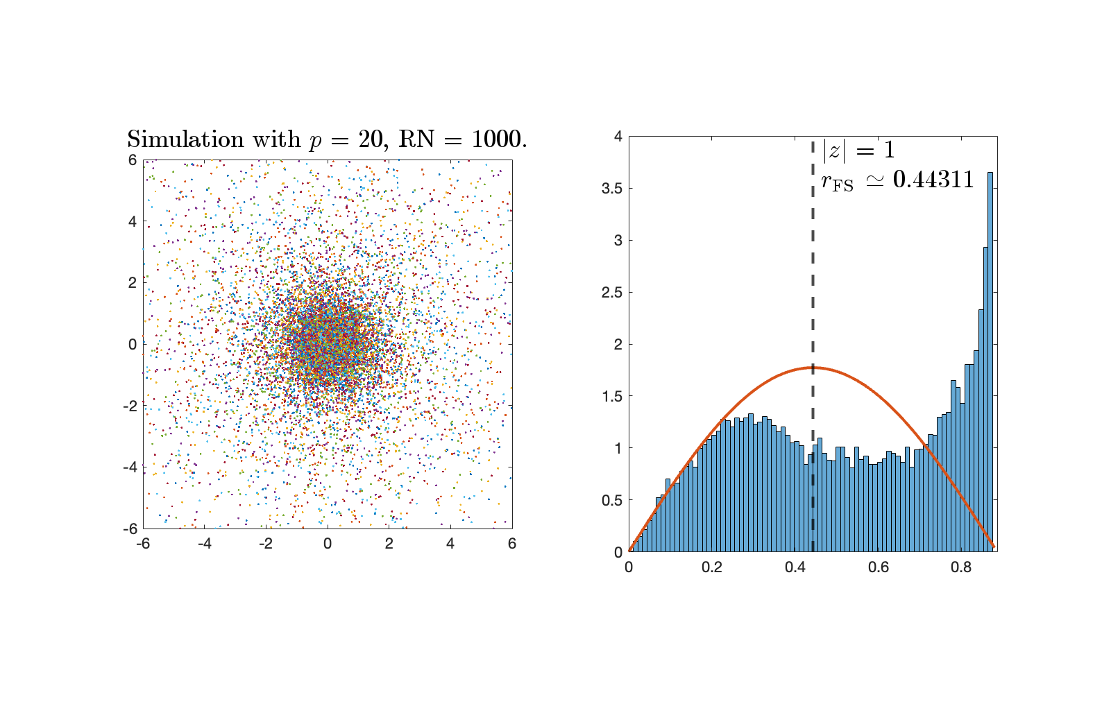
From Figure 1, with , near the origin (inside the support of ), we see the simulated zeros approximate quite well, but outside the support (the part ), the simulated zeros behave very differently from . More simulation results will be given in Section 5.7 to illustrate the convergence results on the support of from Sections 1.3 and 1.4.
From (1.27), the asymptotics of is a crucial term to study . By the asymptotic expansion of (see Theorem 2.9), we conclude that
| (1.45) |
When is smooth and is prequantum (that is ), the lower bounds for were obtained in [21, 22], [1], [26, Proposition 5.16] under the assumption that vanishes only up to order . But a proper lower bound for in general case is missing.
The above expected lower bounds relate clearly to the lowest nonzero eigenvalues of . Let us focus on the non-negative function . For a nontrivial , is injective and positive, set , then on , we get a lower bound for :
| (1.46) |
The easy case is that the essential infimum of is strictly positive on , so that we can conclude uniformly on as .
When a nontrivial has a -vanishing point in , then decays to as (see the analogous statements in Corollary 2.6 and Remark 2.7, see also [29, Proposition 9.2.1]). Then a first step to study is to understand how fast it decays to when vanishes at some points in .
In Section 5.4, for the Hermitian line bundle on the Riemann sphere , we have computed explicitly the Toeplitz spectra for three types of functions and obtain three different asymptotic behavior for . Let denote a standard complex chart for .
-
•
For , set on , then has only one vanishing point at with vanishing order . We have
(1.47) -
•
For on , then has only one vanishing point at with vanishing order . We have
(1.48) -
•
Let be a geodesic ball, set the indicator function for . Assume , hence . We have
(1.49)
In Question 5.13, following the above examples, we summarize a question for the lowest Toeplitz eigenvalues for the general compact Hermitian complex manifolds.
Now we present some partial results on , whose proofs will be given in Section 5.3. A complete answer still remains open.
Proposition 1.22.
Let be a connected, compact Hermitian complex manifold and let , be holomorphic line bundles on with smooth Hermitian metrics. Assume to be positive. Fix which is not identically zero.
-
(i)
For , if there exists such that is near and vanishes at with vanishing order , then there exists such that for all ,
(1.50) -
(ii)
If there exists such that is smooth near and vanishes at with vanishing order , then for any , there exists such that for all ,
(1.51)
The following result provides a supportive evidence for the situation like (1.49), which also refines the lower bound in (1.28) in compact case.
Theorem 1.23.
Let be a connected, compact Hermitian complex manifold and let , be holomorphic line bundles on with smooth Hermitian metrics. Assume to be positive. For which is not identically zero and is continuous near a nonvanishing point, there exist constants , depending only on , , and such that for all ,
| (1.52) |
If , then for any , there exists such that for all ,
| (1.53) |
1.8. Organization of the paper
This paper is organized as follows:
In Section 2, we give the asymptotic expansions of the Berezin–Toeplitz kernels under the local regularity assumption on .
In Section 3, we recall the definition of Gaussian -holomorphic sections given in [26, Section 4] and the related results.
In Section 4, we prove Theorem 1.8, where the key intermediate result is the Proposition 4.6. In particular, we give the proof of Proposition 1.11 in Section 4.5.
In Section 5, we study the asymptotic distribution of random zeros on the support of . In particular, the proofs of Theorems 1.12, 1.14, 1.15 and 1.16 are given. The results on the lowest eigenvalues of for a compact Hermitian manifold are given in Section 5.3.
At last, in Section 6, we discuss the number variance and the asymptotic normality of the zeros of on for a real smooth function with compact support.
Acknowledgments
AD and BL thank NYU Shanghai for their hospitality. We also thank Xiaonan Ma and Stéphane Nonnenmacher for useful discussions.
2. Toeplitz operators and asymptotics of Toeplitz kernels
Let be a connected complex Hermitian (paracompact) manifold of complex dimension , where denotes the canonical complex structure of , and denotes a -compatible Hermitian form. Then we have an induced Riemannian metric on . We denote by the curvature of the Chern connection on with respect to induced Hermitian metric by . Let denote the Riemannian distance of . Let , be two Hermitian holomorphic line bundle on , and let , denote the corresponding Chern connections with the respective curvature forms , . We always assume Condition 1.1 to hold.
2.1. Bergman projections and the asymptotics of Bergman kernels
The Riemannian volume form on is denoted by . For , set . For , the -inner product is defined as follows,
| (2.1) |
Let be the completion of with respect to the above -inner product. Let denote the space of global holomorphic sections of on . We set
| (2.2) |
Then it is a separable Hilbert subspace of . Set
| (2.3) |
Let denote the obvious orthogonal projection, which is called the Bergman projection. It has a smooth Schwartz integral kernel, denoted by . Following the work of Ma-Marinescu [39, Chapters 4 & 6], we have the following results on the asymptotics of Bergman kernels (under the assumption (4.1)):
-
•
(Off-diagonal estimates) For any , , a compact subset , there exists such that for all , , we have
(2.4) Here the -norm is induced by , and , .
- •
Furthermore, the near-diagonal expansion for also holds uniformly on any given compact subset of . To describe this expansion, we need to introduce some notation as follows.
Fix a point . Let be an orthonormal basis of such that
| (2.6) |
where , are the eigenvalues of . We have
| (2.7) |
Set , , . Then they form an orthonormal basis of the (real) tangent vector space . Now we introduce the complex coordinate for (with respect to the complex structure ). If , we can write
| (2.8) |
Set with , . We call the complex coordinate of . Then by (2.8),
| (2.9) |
so that
| (2.10) |
Note that . For , let denote the corresponding complex coordinates. Define
| (2.11) |
Define a weighted distance function as follows,
| (2.12) |
Then
| (2.13) |
For sufficiently small , we identify the small open ball in with the ball in via the geodesic coordinate. Let be the positive smooth function such that
| (2.14) |
where denotes the Euclidean volume form on with respect to . In particular, .
There exists such that for , we have
| (2.15) |
In particular,
| (2.16) |
Moreover, if we consider a compact subset , the constants and can be chosen uniformly for all . Similarly, by (1.12), on a compact subset , we have
| (2.17) |
We trivialize the line bundle on using the parallel transport with respect to along the curve , . Under this trivialization, for ,
| (2.18) |
By [39, Theorems 4.2.1 & 6.1.1], for any compact subset , there exists a constant so that for any , there exists and constant such that for , , multi-indices , with , we have
| (2.19) |
The functions , are given as follows,
| (2.20) |
where is a polynomial in of degree , whose coefficients are smooth in . In particular,
| (2.21) |
The notation means that this term is bounded uniformly by for any given and with some constant which is independent of the choices of , and involved in (2.19).
One crucial step in the approach of Ma-Marinescu [39, Chapters 4 & 6] for the Bergman kernel expansions is the localization the calculation of the Bergman kernel near one given point [39, Section 4.1] due to the finite propagation speed of solutions of hyperbolic equations. For our convenience of explaining the proofs of Toeplitz kernels in next Section, we sketch this localization technique in the sequel.
Let denote the -operator on , and let denote its formal adjoint with respect to the -inner product. We always take the maximal extensions of , as differential operators on . Since is assumed to be complete, then the maximal extension of coincides with the Hilbert adjoint of the maximal extension of . We still use the same notation to denote the above operators.
The Kodaira Laplacian is a densely defined, positive operator. In our setting, it has a unique self-adjoint extension, denoted also by and called Gaffney extension, whose domain is given by
| (2.22) |
Then we have
| (2.23) |
The assumptions in (4.1) implies a spectral gap [39, (6.1.8)] so that there exists , such that
| (2.24) |
Moreover, the higher Dolbeault -cohomology groups vanish for . We are mainly concerned with , which will be denoted simply by in the sequel.
Recall that the injectivity radius is defined in (1.40). Fix . Let be an even smooth function such that
| (2.25) |
Set
| (2.26) |
Then is an analytic even function that also lies in the Schwartz space and .
We always consider the integer to be such that (the constants are from the spectral gap (2.24)). Set
| (2.27) |
It is still an even function. Note that by the functional calculus, we have the operators , well-defined as bounded operators on with smooth integral kernels. In particular, if , we have
| (2.28) |
If are two differential operators of order with compact support respectively, then for any , there exists such that for , we have for any ,
| (2.29) |
As a consequence, the Bergman projection can be approximated by up to an reminder of as well as in the level of their integral kernels. In particular, only depends on the restriction of to , and we have
| (2.30) |
As a consequence, the off-diagonal estimate (2.4) follows from (2.28), (2.29) and (2.30). For the on-diagonal expansion (2.5) and the near-diagonal expansion (2.19), the computation localizes to the small ball . The details are referred to [39, Section 4.1].
Finally, we recall the off-diagonal estimates for on a compact complex manifold.
Theorem 2.1 ([42, Theorem 1] and [17, Theorem 1]).
Let be a connected, compact Hermitian complex manifold and let , be holomorphic line bundles on with smooth Hermitian metrics. Assume to be positive. Then there exist constants and such that for any , there exists a constant such that for , and for all ,
| (2.31) |
Moreover, for any , , there exist constants , such that for all with , , we have
| (2.32) |
The first part of the above theorem was proved by Ma–Marinescu [42, Theorem 1], and their result holds for general (noncompact) complete manifolds with bounded geometry. Under the off-diagonal assumption , for the case where , and trivial line bundle, (2.31) is called Agmon estimate, and also follows from the parametix of the Szegő kernels on pseudo-convex domains (such as [24, 37]), see also [38, Theorem 3.1]. The sharper off-diagonal estimate (2.31) was proved by Christ [17] by studying the near-diagonal estimate of the Green kernels for Kodaira Laplacians acting on -forms.
2.2. Berezin–Toeplitz quantization
We have defined the following spaces of bounded measurable functions in the Introduction:
Definition 2.2.
For any , set
| (2.33) |
where denotes the pointwise multiplication by . The family of bounded operators is called Toeplitz operator associated to the symbol , and we call the Toeplitz operator of level . Equivalently, can be seen as an operator on -spaces, , .
The map which associates to a function the operator on is the Berezin–Toeplitz quantization of level . The map is called the Berezin–Toeplitz quantization [12, 39, 40, 45, 47]. Clearly, we have
| (2.34) |
where denotes the operator norm of .
For and , always has a smooth integral kernel given by
| (2.35) |
Note also that the Hilbert adjoint of is . If has compact support, an easy modification of the arguments in [26, Proof of Proposition 4.7] shows that all , , are Hilbert-Schmidt.
In [39, Chapter 7], the asymptotic expansion of as has been studied in detail with the assumption that is smooth on . However, without the global smoothness of , the same arguments presented in [39, Sections 7.2 & 7.5] can still be utilized to obtain the analogues of [39, Lemmas 7.2.2 & 7.2.4, Theorem 7.5.1]. Note that in [5] Toeplitz operators with symbol were considered (see also [14]), and the asymptotics of their kernels were established using the arguments from [39, Sections 7.2 & 7.5]. In particular, the first part of the following theorem for compact was already given in [5, Lemma 3.1].
Theorem 2.3.
Assume the geometric setting as in Condition 1.1. Given . Then for any compact subset and , there exists such that for and for all , we have the on-diagonal estimate
| (2.36) |
For any , , and a compact subset , there exists such that for with and for all , we have the off-diagonal estimate
| (2.37) |
Let be an open subset such that that is smooth on . There exists a family of polynomials with the same parity as , and smooth in such that for any compact subset , there exist , such that for any , , , multi-indice , with , there exist , such that
| (2.38) |
In particular, we have . For , if vanishes at with vanishing order , then we have for . If , then we have for .
Proof.
By considering the operator defined in previous Section (cf. (2.27), (2.28)), we get by (2.28), (2.29) and (2.33),
| (2.39) |
For any compact subset , for , we have
| (2.40) |
Recalling the definitions (2.25), (2.26) of the functions and , we have by (2.30),
| (2.41) |
Then, using the same arguments from the proof of (2.4) from the estimate (2.29), we get (2.37).
Now let us consider a compact subset and take take in the definition of function in (2.25). Then for and the asymptotic expansion of is the same as , and as in [39, Proof of Lemma 7.2.4], the computations of the expansion only depend on the values of on , then the lack of global smoothness of will not make any difference on this computations near . More precisely, we consider the point , we trivialize the line bundles , on the small ball along the radial geodesics from the center with respect to their Chern connections, so that locally the line bundles , are identified with the trivial line bundles given by , respectively. Under this trivialization, for , , we have
| (2.42) |
We regard , (), as a smooth section function over . We refer to [39, Sections 4.1.5 & 4.2.1] for more details.
Let be a smooth even function such that
| (2.43) |
Then for with , we have
| (2.44) |
where is given as the function in (2.14) but we put the subscript to indicate the base point . Note that in (2.44), we do not need to be smooth near .
To conclude (2.36), we can proceed as in the proof of [5, Lemma 3.1]. Indeed, the derivatives on variable at a given point can be replaced by the derivatives on and in (2.44), which eventually makes derivatives on or of , then the factor follows from (2.19).
Now we assume that is smooth on and is a compact subset of . In the above arguments to obtain (2.44), we take . Following exactly the same arguments in [39, Proof of Lemma 7.2.4], the identity (2.44) gives the expansion (2.38) with for the case .
For general , we note that the expansions of is given by computing the following integration
| (2.45) |
where we apply (2.19) for and . Then (2.38) for general follows from the analogous arguments as in [39, Proof of Lemma 7.2.4] (also cf. [5, Proof of Theorem 3.3]) and a simple observation on [39, (7.1.6) in Lemma 7.1.1]: for polynomials there exists a polynomial such that
| (2.46) |
and for multi-indice , , we have
| (2.47) |
This way, we complete the proof of (2.38).
The formula for general is given by [39, (7.2.16)] inductively when is near , more precisely, we have
| (2.48) |
where is the polynomial in (2.20) of degree . Thus we conclude directly that is a polynomial whose coefficients are given in terms of the derivatives of at up to order , by induction on , we get for if vanishes at up to order . If , we can modify to an equivalent function which is identically near so that they define the same Toeplitz operator, in particular, from again [39, (7.2.16)], we conclude . The proof is completed. ∎
Remark 2.4.
As in [5, §IV], instead of assuming to be smooth on , we can consider an assumption of lower regularity. We have the following result, which is essentially a local version of [5, Lemma 4.2].
Theorem 2.5.
Assume the geometric setting as given in Condition 1.1. Given . For . Let be an open subset such that that is on . For any compact subset , there exists such that for any , , , there exist , such that
| (2.50) |
where the polynomials () are the same as given in Theorem 2.3 but their coefficients are of class in variable .
Proof.
As a consequence of Theorem 2.5, analogous to [39, Lemma 7.4.2], [5, Theorem 5.1 and Remark 5.7] and employing the same arguments in their proof, we also have the following result:
Corollary 2.6.
Assume the geometric setting as given in Condition 1.1. For , if there exists a point such that and is near , then
| (2.51) |
More precisely, there exists a constant such that for ,
| (2.52) |
Remark 2.7.
The following result is an extension of [5, Theorem 3.7], where it is proved for compact case, and the same proof applies in our setting since the (essential) support of is assumed to be compact.
Theorem 2.8 (cf. [5, Theorem 3.7]).
For , then is a trace class. We have the following expansion as : for any ,
| (2.53) |
where , the functions () are given in (2.5).
Let us discuss a bit more on the asymptotics of the spectrum of . We restrict us to the case . Then is a self-adjoint compact operator on . When , the residual spectrum of contains only , and each nonzero eigenvalue in the point spectrum of always has finite multiplicity. When is given as the indicator function of a (Borel) subset of , the asymptotic statistics of the eigenvalues of were studied by [7, 13, 44, 37] in various settings for compact or noncompact . Moreover, for a continuous function with compact support, the spectral densitiy measure of is defined as the sum of the Dirac masses at all the eigenvalues (counted with multiplicities) of , which is locally finite. A result of [35] shows that as , we have the weak convergence of measures on ,
| (2.54) |
This extends the results for compact Kähler manifolds or domains in , such as [7, 37].
In Section 5.3, we will give more results for the asymptotics of the lowest eigenvalues of on a compact Hermitian manifold.
2.3. Compositions of Toeplitz operators
Now we consider the composition (or simply ) of Toeplitz operators for two functions . Based at the previous Section, the following theorem is an easy extension of some results presented by Ma and Marinescu in [39, Theorems 7.4.1 & 7.5.1] and [41, Theorem 0.2].
Theorem 2.9.
Assume the geometric setting as in Condition 1.1. Given . Then for any compact subset , there exists such that for and for all , we have the on-diagonal estimate
| (2.55) |
For any , , and a compact subset , there exists such that for with and for all , we have the off-diagonal estimate
| (2.56) |
Let be an open subset such that that both and are smooth on . There exists a family of polynomials with the same parity as , and smooth in such that for any compact subset , there exist , such that for any , , and multi-indices , with , there exist , such that
| (2.57) |
In particular, we have . If and , then we have for .
Proof.
The proof of this theorem follows from the analogous arguments in the proof of [39, Theorem 7.5.1] and of Theorem 2.3 in previous Section. In particular, for , for with , ( is chosen properly), then we have (cf. [39, (7.4.5)])
| (2.58) |
Then combining (2.58) with (2.36) and (2.49), we conclude the estimate (2.55). Then similarly, by (2.37), we get (2.56). When , are smooth near , the expansion (2.57) follows from the combination of the expansion (2.38), (2.47) and (2.58) by the arguments given in [39, Section 7.4]. Note that an explicit formula for is given in [39, (7.4.7)](see also (2.59)). The proof is complete. ∎
Lemma 2.10.
The polynomial in has degree , and its coefficients are given by polynomials in terms of the derivatives of , at up to order .
Proof.
Remark 2.11.
2.4. Normalized Berezin–Toeplitz kernels; proof of Theorem 1.20
In this Section, we give the proof of Theorem 1.20. Due to the expansion presented in Theorem 2.9, the proof of this theorem is an easy modification of the proofs of [27, Theorems 1.8 and 5.1]. We include the details as follows.
Proof of Theorem 1.20.
Note that since is smooth on an open neighbourhood of , so that we can apply the asymptotic expansion (2.57) for all points . In particular, we have the uniform expansion on ,
| (2.62) |
where is as given in (2.5). Since we assume to be nonvanishing on , then there exists such that for all sufficiently large , we have
| (2.63) |
We start by proving the second estimate of the theorem. One way to see this estimate is from (2.60), where the constant is determined by the constant that appears in the exponential term. In the sequel, we prove it by the arguments in [27, Section 2.3].
Note that is relatively compact in , so is compact and all the results of Theorem 2.9 are applicable for the points in . Let be the sufficiently small quantity stated in the last part of Theorem 2.9 with . Then by (2.56), if is such that , we have
| (2.64) |
For the given , we will determine a constant later on. We fix a large enough such that
| (2.65) |
For , if is such that , then we take advantage of the expansion in (2.57) with , , , , and , in order to obtain
| (2.66) |
Now for , by Lemma 2.10, we have
| (2.67) |
Note that . By (2.13), (2.16), (2.67), and the properties of in Theorem 2.9, together with the fact that , for , we get that
| (2.68) |
where the constant does not depend on . If
| (2.69) |
then we have for ,
| (2.70) |
We may take in our constraint for . Finally, combining (2.62)–(2.70), we get the desired estimate for any .
We next prove the first part of our theorem. For this purpose, we only need to consider sufficiently large such that , or .
In the expansion (2.57), we take , so , where is the complex coordinate for . We infer
| (2.73) |
Since , by (2.67) we infer that for some constant . Note that for as grows.
Now, when has a lower regularity such as with , the above arguments still hold with the bounded choices of . We give the proof of Corollary 1.21 as follows.
Proof of Corollary 1.21.
The inequality (2.64) does not require a specific regularity on due to (2.56). Then by Theorem 2.12, when is of , the arguments (2.66) – (2.70) holds true with and , so that the second part of (1.43) holds. The first part of (1.43) follows from the same arguments as in last step of the proof of Theorem 1.20, i.e., (2.73) – (2.75). This way, we complete our proof. ∎
Note that the upper bound (1.42) is not optimal for , since we have and (here denotes the coordinate derivatives in ). The following estimate is an analog of [49, Proposition 2.8] in our Berezin–Toeplitz setting.
Lemma 2.13.
With the same assumptions in Theorem 1.20 (in particular, is smooth near ), the term satisfies the following estimate: there exists such that for all sufficiently large , , with ,
| (2.76) |
For given , there exist a sufficiently large such that there exist a constant such that for all , , we have
| (2.77) |
3. Gaussian -holomorphic sections via Toeplitz operators
In this section we recall the Gaussian -holomorphic section of a Hermitian line bundle on a complex manifold defined through a given Hilbert-Schmidt Toeplitz operator, this kind of random holomorphic sections were constructed in [26, Section 4], taking advantage of the theory of abstract Wiener spaces.
3.1. Gaussian -holomorphic sections
We now recall the construction of Gaussian -holomorphic sections given in [26, Sections 4.3 and 4.4]. Let be a holomoprhic line bundle on with smooth Hermitian metric . Furthermore, by we denote the space of -holomorphic sections of on , which is a separable Hilbert space with the Hilbert metric given by the -inner product induced by and . Set
| (3.1) |
In this Section, we always assume that and by we denote the Bergman projector.
Let be the space of measurable essentially bounded real functions on with compact essential support. For the Toeplitz operator is Hilbert-Schmidt and self-adjoint. We will consider in the sequel only non-trivial functions .
When , for with compact support, is a linear isomorphism of with strictly positive eigenvalues. When , the residual spectrum of contains only , and each nonzero eigenvalue in the point spectrum of always has finite multiplicity. In particular, the nonzero eigenvalues of form a decreasing sequence of strictly positive real numbers,
| (3.2) |
where denote the nonzero values in the point spectrum of , repeated according to their multiplicities. If furthermore , the eigenvalues are strictly positive.
Next, we introduce
| (3.3) |
which is a Hilbert space, and the sections in are the -holomorphic sections of detected by . We consider the (self-adjoint) Hilbert-Schmidt operator
| (3.4) |
Note that for a notrivial with compact support, is injective and . We furthermore set , and it is immediate that .
The following lemma now is elementary.
Lemma 3.1.
For we have
| (3.5) |
Suppose that (that is, ). In this case, we can choose an orthonormal basis of with respect to the -metric such that
| (3.6) |
On with , the operator is one-to-one and Hilbert-Schmidt, and defines a Hermitian measurable norm on due to [26, Proposition 4.2]. We furthermore denote by the completion of with respect to and set
| (3.7) |
Endowed with the induced norm this is clearly a separable Hilbert space, and using the basis as in (3.6), we have
| (3.8) |
Proposition 3.2.
Assume and . Then the operator extends uniquely to an isomorphism of Hilbert spaces
| (3.9) |
Given , if , we set
| (3.10) |
This unifies the notation for both cases and .
Let be the topological dual space of . If , then it is uniquely determined by the continuous linear functional on on . This way, we regard as a (dense) subspace of , where can be identified with via the -inner product. By a slight abuse of notation we denote by the Borel -algebra of . Then each is a Borel-measurable function from to . For an arbitrary finite dimensional subspace we introduce the notation
| (3.11) | ||||
where is an orthonormal basis of . Gross [31] proved the following result.
Theorem 3.3 (L. Gross [31], see also [26, Theorem 4.3]).
Let denote the measurable norm on as introduced after (3.6). There exists a unique probability measure on such that for any finite dimensional subspace,
| (3.12) |
for all Borel subset of , where denotes the standard Gaussian measure on with respect to the Hermitian metric associated with . The triple is called an abstract Wiener space.
Definition 3.4.
Let be the Gaussian probability measure on given by the pushforward of the probability measure from Theorem 3.3 through the isomorphism in (3.9). This way, we randomize the sections in . A Gaussian (random) -holomorphic section of associated to a nonzero is a random variable valued in with law , i.e., .
When , then , and is exactly the standard Gaussian probability measure on with respect to the -inner product; so is the pushforward of via the isomorphism . For , let denote the random holomorphic section valued in with law , that is
| (3.13) |
where is an orthonormal basis of as in (3.6) and is a sequence of i.i.d. standard complex Gaussian random variables. In this setting, the random section associated to is given equivalently by
| (3.14) |
The following lemma is an easy modification of [26, Lemma 4.12]
Lemma 3.5.
Assume , . For any nonzero , the random variable on defined via
is a centered complex Gaussian variable with variance .
In the case , we consider the orthonormal basis consisting of eigensections of as in (3.6). Setting
| (3.15) |
the form a sequence of i.i.d. standard complex Gaussian random variables. Then our random section associated to is given equivalently by the formula
| (3.16) |
The well-definedness of the sum in (3.16) is already discussed in [26, Proposition 2.1]. Also note that (3.16) then is consistent with (3.13) and (3.14) which treated the case .
3.2. Currents and the Poincaré-Lelong formula
The zero-set of a holomorphic section is a complex analytic set which is in general singular. The analytic tool used to deal with singularities in complex geometry is the theory of currents, introduced by de Rham [20] (see [25, 30] and especially [28] for complete expositions).
Let be a complex manifold of dimension and let be a complex vector bundle on . The space of smooth sections of is denoted by and is endowed with the -topology of uniform convergence of all derivatives on compact sets. The space of smooth sections of with compact support is denoted by and is endowed with the topology of inductive limit of spaces of smooth sections with support on a given compact set. In particular, we denote by the space of smooth -forms with compact support.
The space of -currents on is the topological dual of the space (called test forms in this context). In the sequel, we let be the pairing between a -current and a test form . A -current is called of order if it is continuous in the -topology, equivalently, it extends as a linear continuous functional to the space of -forms of class with compact support.
Definition 3.6.
For an open subset , if is a -current of order (for example, a poisitive -current), we define the following norm of on for ,
| (3.17) |
where runs over all test forms in with .
For any analytic hypersurface , we define the current of integration on by
where is the regular set of (a complex submanifold of codimension ). By a theorem of Lelong ([30, p. 32] [25, III-2.7]) the current of integration on is a closed positive -current (hence a stronly positive -current due to [25, III-1.9]). It is clear that is a current of order on .
Let be a holomorphic line bundle on . For a holomorphic section the divisor of is defined as the formal sum
| (3.18) |
where runs over all the irreducible analytic hypersurfaces contained in , and denotes the vanishing order of along . Let denote the set of zeros of , which is a purely -codimensional analytic subset of . The current of integration (with multiplicities) on the divisor is defined by
| (3.19) |
Assume that is endowed with a smooth Hermitian metric . By the Poincaré-Lelong formula [39, Theorem 2.3.3] we have
| (3.20) |
This important formula is crucial for our purposes. It links the zero-divisor to the curvature and to the logarithm of the pointwise norm of a section, which is analytically easier to tackle and allows the introduction of the Bergman kernel or Berezin-Toeplitz kernel into the picture.
3.3. Expectation of zeros of Gaussian -holomorphic sections
We use the same notation as in Section 3.1. In this Section we always assume with . Let denote the smooth kernel of the operator . We consider the orthonormal basis of consisting of eigensections of as in (3.6), then we have the nonnegative function on ,
| (3.21) |
Similar to the proof of [26, Lemma 4.13], we get that the -current is well-defined on . If we proceed as in [26, Section 2.3], in particular, as in the proof of [26, Lemma 2.6], we conclude the following result.
Lemma 3.7 (Definition of positive current ).
Assume with . The following current is a closed positive -current on ,
| (3.22) |
The base locus of is the proper analytic set
| (3.23) |
Then . Hence is a smooth form if . Moreoever, when , we also have .
Theorem 3.8.
Assume with . Let be the random -holomorphic section of associated to defined in Definition 3.4. Then is random variable valued in the space of -currents on (equipped with weak topology). Moreover, the expectation exists as a closed positive -current on and we have
| (3.24) |
Proof.
For , consider the random -current as follows, for any test form ,
| (3.25) |
It is clear that is a random variable valued in (i.e., a measurable function on the underlying probability space). Moreover, by (3.20) and dominated convergence, we have
| (3.26) |
Therefore, is a random variable, and then is a well-defined random variable valued in the space of -currents with respect to the weak topology.
4. Asymptotics of random zeros of -holomorphic sections
Let us recall the main assumption in the semi-classical limit – Condition 1.1 – as follows: we always assume to be a complete Riemannian manifold, and that there exist , such that
| (4.1) |
If is compact and is positive, then the above conditions always hold true. Due to our assumptions on and , for , we have . We may assume that for all .
Definition 4.1.
For , let denote the random -holomorphic section of associated to the nontrivial defined in Definition 3.4.
The goal of this section is to study the asymptotic behavior of the zeros of random section as , where the asymptotic behavior of is a crucial ingredient. As we saw in Section 2, in order to analyze in the semi-classical limit, we always need to assume certain regularities on .
We start with the following lemma, which enable us to apply the results from Section 3 for the line bundles . Recall that the function is given in (2.5).
Lemma 4.2.
For , if there exists an open subset such that and never vanishes on , then for all sufficiently large , we have , hence .
Moreover, fix a proper open subset of , we have
| (4.2) |
Proof.
If , then for all , . Since , we can apply Theorem 2.5 to on so that fix , we have
| (4.3) |
By our assumption , then for all sufficiently large , . Therefore, we have .
4.1. Bounded measurable functions and their supports
This Section is a preparation for the proof of Theorem 1.8. Recall that the quantity for is defined in Definition 1.7. Now we give some examples of function such that has a good geometric sense.
Example 4.3.
-
i)
For , set . Now fix and , let be the open ball in with radius , and define for ,
(4.5) Then is smooth almost everywhere on , and we have for ,
(4.6) In Figure 2, it shows the support in black blocks of the function (that is, , ) on .
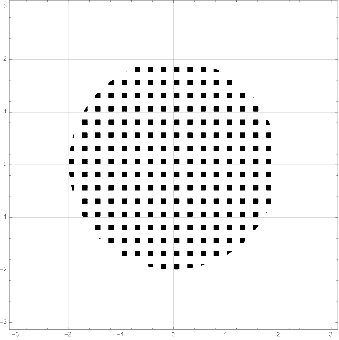
Figure 2. Support of on plotted as black blocks -
ii)
Let be a finite collection of disjoint geodesic open ball of respective radius in a compact Hermtian manifold , set , then is a function which is smooth almost everywhere on , and .
-
iii)
Let be a compact Riemann surface with a Kähler form . Let be the -skelton of a (smooth) triangluation of . Then for a sufficient small , let be the closed subset defined as the -neighbourhood of in (which is still a proper subset). This is a thick graph embbeded in . Then we can use the quantity to quantify the approximation of the thick graph to . Taking a sequence of strict refinements of and a suitable decreasing sequence of , then the sequence of the quantities will converge to .
Let denote the standard Riemannian metric on given by the standard Euclidean inner product on . The following proposition is elementary.
Proposition 4.4.
For every compact subset there exist constants , such that for every point , the open geodesic ball in is always included in a connected, open holomorphic local chart centered at such that is a biholomophism between the open subset and with the following properties:
-
•
, and ;
-
•
is a convex domain of ;
-
•
let be the distance function on associated to the Riemannian metric , then for any ,
(4.7)
As a consequence, for a given , and for , we have
| (4.8) |
where is the number defined as in (1.14) with respect to the standard Riemannian metric on .
Remark 4.5.
The choices of for a given in Proposition 4.4 are not unique, in fact we can always make as small as we want. Moreover, if we take a sufficiently small , then the constant will be very close to .
4.2. A concentration estimate; proof of Theorem 1.8
In this section, we prove Theorem 1.8 which provides a general concentration estimate for the difference between the zeros of the random section and the expected limit on a given domain, provided that the function is supported on the large part of this domain. Recall that the norm for the -currents is given Definition 3.6 with , and that the quantity defined in (1.13), then Theorem 1.8 is a consequence of the following proposition.
Proposition 4.6.
With the same assumption in Theorem 1.8 for and for the line bundles . Fix a pair of nonempty open subsets of with , then there exists a constant such that which is of almost everywhere on with
| (4.9) |
then , and for any , we have a constant such that for all sufficiently large
| (4.10) |
Now we explain how to get Theorem 1.8 from Proposition 4.6, and the proof of Proposition 4.6 is defered to Section 4.4.
Proof of Theorem 1.8.
Combining the first part of Proposition 4.6 with Lemma 4.2, we get that for all sufficiently large , , that is . Then the results from Section 3 apply. In particular, the random section is not the zero variable.
The Poincaré-Lelong formula (3.20) shows that
| (4.11) |
as an identity of -currents on Let be the open subset as assumed in Theorem 1.8. Now fix with (that is, ). Note that . Then
| (4.12) |
Since has a compact support in , so has . Then
| (4.13) |
Applying Proposition 4.6 to get a constant , we fix a as in the theorem with
then . When we take
we can always fix a sufficiently small such that
Since the term converges to as , then there exists an integer (depending on ) such that for any and all ,
| (4.14) |
Applying Proposition 4.6 to right-hand side of (4.13) with , we get
| (4.15) |
For , except the event from (4.15) of probability , we have for all ,
| (4.16) |
Equivalently, except the event in (4.15) of probability , we have
| (4.17) |
This way, we get (1.16). To prove (1.17), applying Borel-Cantelli lemma to (1.16), we get
| (4.18) |
By taking a sequence of ’s that decreases to , we infer (1.17) from (4.18). ∎
4.3. Local sup-norms of random -holomorphic sections
Before proving Proposition 4.6, we need to investigate the probabilities for taking both atypically large and small values, respectively. We follow the same strategy as in [26, Section 3.3].
Let be a relatively compact open subset. For , we set
| (4.19) |
Proposition 4.7.
Assume Condition 1.1 to hold. Fix . Let be a relatively compact open subset, then for any , there exists a constant such that for ,
| (4.20) |
Proof.
We fix and let be sufficiently small so that we can choose a finite set of points such that the geodesic open balls , , form an open covering of . Since is sufficiently small, then we can assume that each larger ball lies in a complex chart (hence viewed as an open subset of ), and that for each , we can fix a local holomorphic frame (resp. ) of (resp. ) on a neighborhood of with and . Set
| (4.21) |
It is clear that . By fixing small enough, we can and do assume that
| (4.22) |
Then there exists a constant such that for each , if is a holomorphic function on a neighborhood of , then
| (4.23) |
where the volume form on is used in the norm . Note that the choices of , , , and the constants , are independent of the tensor power . Set . For , on each , we write
| (4.24) |
where is a holomorphic function on the chart in corresponds to . Then we have
| (4.25) |
where the constant independent of is determined by
The next step is to estimate the quantity for . Applying Hölder’s inequality with , we get
| (4.26) |
For , let be an orthonormal basis of with respect to -inner product and consisting of eigensections of with nonzero eigenvalues . As explained in (3.16), we can construct a sequence of i.i.d. standard complex Gaussian variable such that we can write
| (4.27) |
As in (4.23), on a neighborhood of , write
| (4.28) |
If , set
| (4.29) |
Then is a complex Gaussian random variable with (total) variance . By our assumption on the local frame , we get
| (4.30) |
Then we have
| (4.31) |
As a consequence, we get that for ,
| (4.32) |
Since we are in the context of -finite measures and the integrands are non-negative, Tonelli’s Theorem applies, so that
| (4.33) |
Moreover, by the estimate for given in (2.55) on a compact subset, there exists a constant (independent of ) such that for , ,
| (4.34) |
Combining (4.26) with the above inequalities, we infer that
| (4.35) |
By applying (4.25) to , we get
| (4.36) |
where is a constant independent of . Then (4.20) follows from Chebyshev’s inequality and the inequality from (4.22). ∎
Now we consider the probabilities of small values of , and we will adapt the ideas in [51], [27, 26]: viewing as a line bundle valued holomorphic Gaussian field on and studying its correlation function.
Proposition 4.8.
Proof.
From the local uniformity of the Berezin–Toeplitz kernel expansions, as explained in Section 2.3, it follows that for every compact subset there exists such that for all and all we have .
Now for any we fix some , with , and set
| (4.38) |
whenever . Then is a complex Gaussian random variable. Moreover, for any two points , we have
| (4.39) |
where is defined by (1.39).
Since , so we can find a small open ball , then is and never vanishes near . Then the asymptotic equations in (1.43) from Corollary 1.21 holds true for all and for all . In particular, we have
| (4.40) |
Next step, by (1.43), we may proceed using the similar arguments in [51, Section 3.2] or [27, Subsection 3.3 and Theorem 1.13], we can prove a more general version of (4.37) as follows: for a sequence of positive numbers ,
| (4.41) |
Then, for any , choosing in (4.41), we recover (4.37). This completes our proof. ∎
Corollary 4.9.
Let be a connected Hermitian complex manifold and let , be two holomorphic line bundles on with smooth Hermitian metrics. Assume Condition 1.1 to hold. Fix and assume that on a small open ball of , is and nonvanishing. Let be a relatively compact open subset in such that , then there exist constants such that for all and ,
| (4.42) |
4.4. Proof of Proposition 4.6
Now we give the proof of Proposition 4.6, which follows by combining from the arguments in [51, Section 4.1] with Corollary 4.9. Since the kernels behave in a more complicated way, depending on the values of , than the Bergman kernels, some steps are required necessary modifications from that in [51, Section 4.1]. In the same time, we also include several explicit function estimates in order to work out a rough formula for the quantity in the statement of Proposition 4.6.
Proof of Proposition 4.6.
For , set
| (4.43) |
Then
| (4.44) |
Let be the open subset as assumed in the proposition. Then for any nonzero holomorphic section , we have that is integrable on with respect to . We now start with showing that for any ,
| (4.45) |
For this purpose, observe that on we have
| (4.46) |
which then supplies us with
| (4.47) |
where denotes the volume of with respect to .
Note that we assume that is of class with almost everywhere near and with
the set , by its definition, can not be null measure in any given open subset, then there exists a small open ball such that is of class (since ) and never vanishing on . Therefore, Corollary 4.9 applies to this open subset of and the function . Then combining (4.47) with Corollary 4.9, we obtain (4.45) with any given .
The next step is to study . At first, let us construct a particular family of holomorphic local charts to cover . Since is relatively compact in , we apply Proposition 4.4 for to choose the constants such that the -neighbourhood of is still included in and the line bundles , can be locally trivialized on any small (geodesic) balls of radius on .
For each point , let be the local chart as in Proposition 4.4. Set
| (4.48) |
Then the family is an open covering of , hence there exists a finite number of points such that is already an open covering of . We also set
By (4.8), we have
| (4.49) |
For , any open coordinate ball (of ) in of radius intersects the essential support of .
Next we work on each . In order to simplify the notation, after rescaling the coordinates of the local chart , we may and we will consider the following model case: in the local coordinate , set , and . Assume that on the coordinate open ball , the holomorphic line bundles and can be trivialized by holomorphic local frames. In the following, we work on this coordinates and let denote the number given as in (1.14) with respect to the standard Riemannian metric on .
For which is of almost everywhere near with , we always have .
Let , the be respective holomorphic local frames of the line bundles , restricting to the open ball . Set , . On this local chart, we can write
| (4.50) |
where is a random holomorphic function on . Then on
| (4.51) |
Fixing , we take
| (4.52) |
Then by (4.45) and (4.51), we get that, except the event of probability less than , we have for all ,
| (4.53) |
where denote the invariant probability measure on the sphere .
For , consider the Poisson kernel for the ball ,
| (4.54) |
where , . Since is a subharmonic function on , by the sub-mean inequality in terms of Poisson kernel, we conclude that for any point , ,
| (4.55) |
As a consequence, we have, for ,
| (4.56) |
Note that , following from the condition , Corollary 4.9 applies to . We conclude that except for an event of probability less than , we can always find a point with the property:
| (4.57) |
Then combining it with (4.53) and (4.56), we get that except for an event of probability less than , we have that for all ,
| (4.58) |
where is a sufficiently large constant given by
Given (the case of will become a consequence of this one), we fix a decomposition of the unit sphere into a disjoint union of sets , , , with (Euclidean) diameter . The number is a large integer depending on . The following inequality was established in [51, (4.4)]: there exists a constant independent of such that for any , any collection of points with and any subharmonic function on ,
| (4.59) |
The main idea to prove (4.59) in [51, Section 4.1] is to use the Poisson kernel as in (4.55) for each term , and is a constant related to the estimate on the derivatives of , and in our setting, we can take .
From this point we proceed as in [51, Section 4.1, pp. 1992] but with some necessary modifications, and we will also produce a rough formula for the constant needed in our proposition. Fix , and let which is of almost everywhere near such that .
Set and set , for . Then for , , set
| (4.60) |
Then form a covering for , moreover, each always contains a coordinate open ball of raidus , so that Corollary 4.9 applies: there exists such that for all
| (4.61) |
Set the event , then we have that for ,
| (4.62) |
When lies outside , we can always find with
| (4.63) |
Fix , there exists such that
Then , so that we have
| (4.64) |
A similar inequality holds also for . Moreover, we have , then we can apply (4.59) for . We combine this with (4.58), so when lies outside , we have
| (4.65) |
We set
| (4.66) |
Let be such that for all , , where denotes the standard Lebesgue measure on . Then taking the integral with repsect to and rescaling to the standard spherical measure for the sphere of radius , we conclude, by taking advantage of (4.65), that
| (4.67) |
Combining the above estimate with (4.45), we get that for ,
| (4.68) |
4.5. Expected mass of random -holomorphic sections
Recall that the volume form that is used to define the -inner products is . Similarly, since is uniformly positive on we define a different volume form on ,
| (4.72) |
where the positive function on is given by (2.7).
Recall that for a holomorphic section we introduced the measure on in Definition 1.10. The following proposition gives preliminary results on the expectation of mass distribution of . The proof follows from the asymptotic expansion of given in Section 2.
Proposition 4.10.
Let be a connected Hermitian complex manifold and let , be two holomorphic line bundles on with smooth Hermitian metrics. Assume Condition 1.1 to hold. Fix a nontrivial , or for a relative compact domain with a continuous boundary, and let be the associated random -holomorphic sections defined via . Then for any , we have
| (4.73) |
Hence we have the locally uniform weak-star convergence of measures on ,
| (4.74) |
Proof.
The identity (4.73) follows from the series formula for given in (4.27) (see also (3.16)). Then for any function , we have
| (4.75) |
When , by Theorem 2.12, we have
| (4.76) |
Now we consider the case . Fix a function and let be a compact subset with . By (2.36), we have for
| (4.77) |
with some constant . For any , let be a small number such that
| (4.78) |
By the uniform expansion of Theorem 2.12 for the points away from , we get that there exits such that for all
| (4.79) |
where .
Assembling the above estimates together we have for ,
| (4.80) |
Then we conclude that
| (4.81) |
The proof is complete. ∎
We need the following lemma to prove Proposition 1.11.
Lemma 4.11.
With the same assumptions as in Proposition 4.10 for the geometric data, let be a relative compact open subset of , and fix a nontrivial . Then for any , set , we have
| (4.82) |
Proof.
Proof of Proposition 1.11.
By Proposition 4.10, we have
| (4.86) |
Then as , we have
| (4.87) |
Note that is a sequence of independent variables, and by Lemma 4.11, we have , so that by the strong law of large numbers for pairwise independent random variables (see [19, Theorem 1]), we have
| (4.88) |
Combining the above convergence with (4.87) we conclude the proof. ∎
5. Expectation and equidistribution on the support of the symbol
We continue our discussion of zeros of in Section 4, especially, we prove that the random zeros will be asymptotically uniformly distributed with respect to on parts inside the support of where it is with . These results are applications of Theorem 1.8 specializing to the case .
5.1. Equidistribution of random zeros on the support; proof of Theorem 1.14
In [26, Section 5], the zeros of random sections were studied for the case , and the equidistribution results were proven for their zeros as on the support of with the assumption that vanishes up to order . Here, we remove the condition on the vanishing orders of for the equidistribution results.
Proof of Theorem 1.12.
Proof of Theorem 1.14.
Note that the estimate (1.26) is a direct consequence of (1.25) by taking . Hence, it is sufficient to prove (1.25). For this purpose, let denote the indicator function of on . Let be arbitrary, and take , with supports in such that and
| (5.1) |
Note that the existence of such functions is guaranteed by the assumption that has measure with respect to , hence also to . For set . By applying Theorem 1.12 to separately, we get exactly (1.25). ∎
Another interesting object that is closely related to this equidistribution result is to study the asymptotic behavior of and compare it with , the expected limit. By Lemma 3.7 and Theorem 3.8, we have
| (5.2) |
Now we show that, under a global finiteness on the geometry of the manifold, the convergence of to on can be obtained as a consequence of the equidistribution result (1.21). Certainly, this is a weaker version of the convergence given in Theorem 1.16 via the method of pluripotential theory on .
Proposition 5.1.
We assume the same geometric conditions on as in Theorem 1.12. Furthermore, we assume one of the following conditions to hold:
-
(i)
is Kähler and , or
-
(ii)
.
Fix . Let be an open subset of such that , and we assume that is of class almost everywhere on . Then we have
| (5.3) |
where the limits in (5.3) are taken with respect to the convergence of -currents on .
Proof.
Applying Theorem 1.12, we get that for any , we have
| (5.4) |
Now we assume that first case: is Kähler and . For all , , due to the positivity of the current , we have
| (5.5) |
and the last identity follows from the Poincaré-Lelong formula. We may set , then
| (5.6) |
Then applying the dominated convergence theorem to the limit in (5.4), we infer that
| (5.7) |
By the definition of , we can rewrite the above limit as
| (5.8) |
This way, we get the first line of (5.3).
For the second case , we just replace by in the above arguments, and certainly we have to change the -norm for test forms to the one induced by , then we conclude the same conclusion (5.3). This way, we complete our proof. ∎
5.2. Proofs of Theorems 1.15 and 1.16
Now we give a general result on that is obtained from the pluripotential theory on .
Let us recall some basic facts about the plurisubharmonic functions. Let be a connected complex manifold of complex dimension , and we fix a smooth Kähler form on . Recall that a quasi-plurisubharmonic (quasi-psh for short) function on an open domain of is locally the difference of a plurisubharmonic function and a smooth one. For any open subset , set the space of quasi-psh functions on with respect to , that consists of the upper semi-coutinuous functions with the propoerty as -current on , where .
The following two propositions are well-known facts for the functions in , which follow from the corresponding properties of plurisubharmonic functions on the domains of . For their proofs, we refer to [33, Theorems 3.2.12, 3.2.13 and 4.1.8].
Proposition 5.3.
Fix an open domain in , and a compact subset . Let be a family of quasi-psh functions on such that for each , , then is a bounded subset in (), and it is also a relatively compact subset of .
Proposition 5.4.
Let be a relatively compact open domain in . Let () be a sequence of quasi-psh functions on with on , which have a uniform upper bound on . Then, only one the following situations holds
-
•
either converge uniformly to on any compact subset of , or
-
•
there exists a subsequence converges in -norm () on to a quasi-psh function on with .
The above propositions allow us to establish some estimates on the integrals of Berezin–Toeplitz kernel function , and then we can deduce the properties on . At first, we give the proof of Theorem 1.15.
Proof of Theorem 1.15.
With our assumption on , by Lemma 4.2, we get for all sufficiently large , then we have the corresponding random -holomorphic section which is not identically zero. By Theorem 3.8, we have the identity of -currents on for :
| (5.10) |
Let be a constant such that on . Then for all , we have
| (5.11) |
Set
| (5.12) |
and we work on the connected compact subset . Then by (5.10) and (5.11), is a quasi-psh function with respect to the Kähler form on , that is, on . Set now
| (5.13) |
Then applying (2.55) on and Theorem 2.12 for the open subset , there exist constants , such that for all ,
| (5.14) |
Therefore is a family of quasi-psh functions on (actually on an open neighbourhood of ) such that each one has the maximum in . By Proposition 5.3, we conclude that is a bounded set in with any . In particular, there exists a constant such that for all , we have
| (5.15) |
As a consequence, for all , we get
| (5.16) |
Then for any nonempty open subset , we have
| (5.17) |
We conclude that for all ,
| (5.18) |
Then considering the probability space modelled as and applying Jensen’s inequality with , we get
| (5.19) |
Combining it with (5.18), we get
| (5.20) |
Therefore, we get exactly (1.28).
The estimate (1.29) follows from combining (5.2) and (5.16) for any test function in . Finally, since the quasi-psh functions form a bounded set of hence relatively compact by Proposition 5.3, then there exists a subsequence which converges in to a quasi-psh function . Then applying (5.10), we get (1.30). In particular, since converges uniformly to on , we also have . This way, we finish our proof. ∎
When with some constant , the lower bound in (1.28) is trivial due to the asymptotic expansions of Bergman kernel function . When vanishes identically on a nonempty open subset of (which is given as in Theorem 1.15), by Theorem 2.9, we have
| (5.21) |
In this case, the lower bound in (1.28) is nontrivial and provides a better understanding of the decay of on .
Following the properties introduced in the proof of Theorem 1.15, we can generalize Proposition 5.1 to obtain the convergence of on the support of .
Proof of Theorem 1.16.
We use the same notation as in the proof of Theorem 1.15. Note that is compact in . Since is of class almost everywhere near and it has nonvanishing points, then the family defined in (5.12) is a bounded set in following Proposition 5.3. Let be the constant such that for all ,
| (5.22) |
As a consequence, for any measurable, we have
| (5.23) |
Combining this with the fact that is a bounded in , we get that the family is uniformly integrable on (see [11, Definition 4.5.1 and Proposition 4.5.3]).
By Theorem 2.12, the assumption on implies that converges to almost everywhere on with respect to the Lebesgue measure (or ). Finally by the Lebesgue-Vitali theorem (see [11, Theorem 4.5.4 and Corollary 4.5.5]), we get that converges to in -norm on , and (1.31) follows. Combining (5.10) with (1.31), we conclude the convergence (1.32). The proof is complete. ∎
Remark 5.5.
(i) If we use the bound of -norm for such as (5.22) in the proof of Theorem 1.15, then we replace the exponent in the right-hand side of (1.28) by .
(ii) In Theorem 1.16, if we assume a stronger condition on , for example, if the function is integrable on with respect to , then one can ask if the following convergence of -currents on as holds,
| (5.24) |
5.3. Random zeros and lowest Toeplitz eigenvalues on compact manifolds
Now we apply the results from previous Sections to the case of compact complex manifolds. In this Section, we always assume to be a connected compact Hermitian manifold and to be a positive holomorphic line bundle on . A random section as in (1.7) can be equivalently defined by (1.44).
Theorem 5.6.
Let be a connected, compact complex Hermitian manifold and let , be holomorphic line bundles on with smooth Hermitian metrics. Assume to be positive. Fix a real bounded function which is of class almost everywhere on and with (or equivalently ). Then we have -a.s. that
| (5.27) |
If is a real bounded function which is almost everywhere on and with , then as , we have
| (5.28) |
and
| (5.29) |
Remark 5.7.
Proposition 5.8.
Let be a connected, compact complex Hermitian manifold and let , be holomorphic line bundles on with smooth Hermitian metrics. Assume to be positive. Fix a real bounded function (it can take negative values) which is of class almost everywhere on and with (or equivalently ). Then there exists a constant and a decreasing sequence of strictly positive numbers with limit which depend only on , and such that for all , any sequence of nonempty open subsets of , we have
| (5.30) |
Proof.
Theorems 1.12 and 1.16 seem to indicate is that the asymptotic behavior of the random zeros of depends mainly on the support of the function rather than the precise values of . Following this thread, we formulate some interesting questions. For the sake of simplicity, we will restrict ourselves to to consider only non-negative functions , unless explicitly stated otherwise.
At first, we consider the following equivalence relation on the non-negative functions on : for (resp. ), we say they are comparable if there exists a constant such that on whole ,
| (5.34) |
Let (resp. ) be the set of all equivalent classes of comparable functions in (resp. ), then it has a semigroup structure given by the pointwise addition of functions with the zero element given by the zero function.
Lemma 5.9.
If are comparable, then they have exactly the same set-theoretic support, that is , therefore .
On can then enquire about the relation between the asymptotic behaviors of the random zero sets and in the case when , are comparable functions on , which might not be fully supported on .
Question 5.10.
Let be a connected, compact complex Hermitian manifold and let , be holomorphic line bundles on with smooth Hermitian metrics. Assume to be positive. Fix the sequence of the standard Gaussian random holomorphic sections . If two nontrivial functions are comparable, is it true that -a.s.,
| (5.35) |
and that
| (5.36) |
hold true?
By Theorem 5.6, when have full support on , then the above two equations hold true. So the difficult case is when s are not fully supported. Note that if the results hold in general, they allow us to classify the asymptotic behavior of the random zeros associated the function via their equivalence class in .
A potential approach to a positive answer to Question 5.10 is via establishing the following pointwise estimates for a pair of comparable functions for all ,
| (5.37) |
Note that the condition (5.34) only implies
| (5.38) |
which, in general, could not infer (5.37). Moreover, near the nonvanishing smooth point of , inequality (5.37) always holds true for sufficiently large after taking a bit large constant (by the asymptotic expansion (2.57)).
Another interesting question closely related to (5.37) or (5.38) is to understand the asymptotic spectra of or as ; this is already partially addressed in Section 1.7 and the last part Section 2.2. Then in the sequel, we will try to understand more how the lowest eigenvalues of decay to as when has vanishing points.
We start with a lemma for comparison of eigenvalues of Hermitian matrices.
Lemma 5.11 (Weyl’s inequality, see [34, Theorem 4.3.7]).
For . Let , be two Hermitian -matrices, and let be the increasingly ordered eigenvalues of a Hermitian matrix, then we have the inequalities for the eigenvalues, for ,
| (5.39) |
whenever the subscript makes sense.
As a consequence, we have the following comparison results for the eigenvalues of Toeplitz operators.
Lemma 5.12.
Let be a connected, compact complex Hermitian manifold and let , be holomorphic line bundles on with smooth Hermitian metrics. Assume to be positive. Let be such that each of them is not identically zero and . For , let denote the ordered eigenvalues of respectively. Then we have for all , ,
| (5.40) |
As a consequence, if are comparable as in (5.34), then we have for all , ,
| (5.41) |
Proof.
Among all the eigenvalues of , we now concentrate on the lowest nonzero one. These lowest eigenvalues are also interesting in the sense of their correspondence to the lowest energy for the ground state in the Berezin–Toeplitz quantization as in the work of Deleporte [21, 22]. He obtained the asymptotic expansions for as well as for the corresponding eigensections when is a smooth function with only nondegenerate vanishing points of order . Then the general results about the lowest eigenvalues are expected, so that we put it as the following conjecture/question:
Question 5.13.
Let be a connected, compact complex Hermitian manifold and let , be holomorphic line bundles on with smooth Hermitian metrics. Assume to be positive. For (it can take negative values), set (where denotes the vanishing order of at ), show that as
| (5.43) |
where is some constant depending on , and , the sign means up to a multiplication of some nonzero constant. Moreover, a related interesting question is to describe the corresponding eigensections on . Note that in Section 5.4, we give the examples on where the lowest eigenvalues of are the cases listed in (5.43). Following the results on the off-diagonal decay of given in [15, 16, 17, 46, 23], it is possible that we need to assume the analyticity on and , to get the three nice cases in (5.43).
The results in Proposition 1.22 and Theorem 1.23 shows a partial answer to the above question for a non-negative function . In the sequel, we give their proofs as consequence of Theorems 2.1, 2.3, 2.5 and the pluripotential theory on .
Proof of Proposition 1.22.
In both case, we set , since is nontrivial, we always have . In the same time, we have the global point-wise estimate on for all ,
| (5.44) |
that is
| (5.45) |
Remark 5.14.
We also have a uniform lower bound for by an explicit calculation on in (5.46): in fact, we have
| (5.47) |
where is a constant depending only on which is if each component of is even, and is otherwise. As a consequence, if and vanishes on with the vanishing order at most , then there exists such that for all , ,
| (5.48) |
See also [26, Proposition 5.6]. Using instead the expansion (2.57) and Theorem 2.12, one can prove the analogous results of (5.48) for with a general function which might take negative values, see also [26, Proposition 5.16].
Proof of Theorem 1.23.
Let denote a very small (nonempty) open ball in , and we consider the case , the indicator function for . In this case, , and we know is injective and positive for all .
Now we set . For each , there exists a section with and
| (5.49) |
Now we consider the family of integrable real functions on . As a consequence of Poincaré-Lelong formula, , and this family of quasi-psh functions is bounded uniformly from above because of the uniform asymptotic expansion of on .
Now we prove that is a bounded subset of . If it is not true, we can assume that there exists a subsequence such that
| (5.50) |
Then we apply Proposition 5.4 to this subsequence and , we conclude that has to converge uniformly to on , but this contracts to our condition . Therefore, there exists a constant such that for all ,
| (5.51) |
Hence
| (5.52) |
Similar to (5.19), we get
| (5.53) |
Then combining the above inequality with (5.49), we conclude
| (5.54) |
This shows that (1.52) holds with . In general, by our assumption on from the statement, we can always find a small nonempty open ball and a constant such that , then (1.52) follows from Lemma 5.12 for minimal eigenvalues and (5.54).
Now we prove (1.53), we use the technique of choosing coherent sections and the estimate (2.32). Assume now , then we fix and a sufficiently small such that the small geodesic ball . We also assume that the line bundle and can be trivialized over . Let , denote the respective unit (smooth) frames of , , a coherent section associated to , is the unique section such that for any , we have
| (5.55) |
In fact, we have . Then we have
| (5.56) |
and
| (5.57) |
Remark 5.15.
As a consequence, we get the uniform point-wise lower bound for on a compact manifold .
Corollary 5.16.
Definition 5.17.
For any nontrivial , we set
| (5.63) |
By Theorem 1.23, the limit always exists (that is, finite) and is nonpositive. For , we set .
The following result is an easy consequence of Lemma 5.12.
Proposition 5.18.
When is a continuous function on and never vanishes, we have . If , are comparable in the sense of (5.34), then we have
| (5.64) |
This way, we define a function .
5.4. Examples and simulations on Riemann sphere
In this Section, we present the examples of the Toeplitz operators on , in particular, we give the explicit computations on their spectra. In the last part, we present the random zeros of the sections given by certain Toeplitz operators acting on the -random polynomials on .
Let us start with our basic settings. We consider one standard chart for . In this chart, the Fubini-Study metric is given by
| (5.65) |
It is also the volume form on that we will use.
For , let denote the holomorphic line bundle on of degree . Then , we equip with the standard Fubini-Study Hermitian metric and equip with the induced Hermitian metric. Then .
On this chart, the global holomorphic sections of are given by all the polynomials in with degree , i.e.,
| (5.66) |
The canonical orthonormal basis of with respect to the -inner product is given by
| (5.67) |
Note that acts on holomorphically and transitively. On the chart the action is given by
The action of always lifts to and preserves the metrics and . In particular, acts on isometrically with respect to -inner product.
5.5. Lowest eigenvalues of Toeplitz operators for fully supported functions
In this part, we compute the spectra of Toeplitz operators associated to some special functions, as examples for the first two cases listed in (5.43).
Example 5.19.
For , on , we take the function
| (5.68) |
Then is a smooth nonnegative function on with the only vanishing point at , and the vanishing order is .
At first, we have for , then
| (5.69) |
Then we have
| (5.70) |
By elementary techniques on the integrals, we get
| (5.71) |
It is clear that this quantity increases as grows. Then we have the following smallest () and biggest () eigenvalues of :
| (5.72) |
In particular, we have, as ,
| (5.73) |
The corresponding eigensection is .
Example 5.20.
On , we take the function
| (5.74) |
Then is a smooth nonnegative function on with the only vanishing point at , and the vanishing order is , but we have .
Similar to (5.69), for , we have
| (5.75) |
Then we have
| (5.76) |
By elementary techniques on the integrals, we get
| (5.77) |
where denotes the Tricomi confluent hypergeometric function, that is defined as
| (5.78) |
Then we can rewrite
| (5.79) |
A direct computation shows that
| (5.80) |
For the biggest () eigenvalues of , we have the following explicit formula
| (5.81) |
For the smallest eigenvalues, we have
| (5.82) |
Now let us give the asymptotic behavior of as . At first, we have
| (5.83) |
where the second term follows from finding the maximum of . Using the fundamental inequality for ,
| (5.84) |
we get (for all sufficiently large )
| (5.85) |
For the lower bound, we get
| (5.86) |
where the last estimate follows from (5.84).
5.6. Spectrum of Toeplitz operators for indicator functions
For , set the function on as
| (5.89) |
where denotes the indicator function for the open disc of radius . In the sequel, for or , let denote the Fubini-Study volume of . In particular, we have
| (5.90) |
This disc is a geodesic ball in with radius (with respect to Fubini-Study metric).
Now we consider the Toeplitz operators acting on .
Proposition 5.21.
The spectrum of is given by where
| (5.91) |
Moreover, we have
| (5.92) |
For , the -eigenspace is spanned by (hence is -dimensional).
Proof.
By definition, we have
| (5.93) |
where denotes the hypergeometric function . Using the fact that and are non-negative integers, the value of can be worked out explicitly so that we get exactly (5.91). The rest part is clear. ∎
Using the -symmetry, we get the following corollary.
Corollary 5.22.
Let be a nontrivial geodesic ball in with , then we have
| (5.94) |
In particular, if , then decays exponentially to as .
Finally, as a consequence of Lemma 5.12, we get
Proposition 5.23.
For a , if there exists two geodesic ball and two constants such that
| (5.95) |
Then we have for ,
| (5.96) |
In particular, when , decays exponentially to as .
5.7. Simulations of random zeros on the support of the symbol
In this part, we present some simulation results for the zeros of on , where the function is given as in Sections 5.5 and 5.6.
We now explain our computation model. Fix a concrete choice of as above, we already know the precise spectrum of : for , let be the eigenvalues of with the eigensection . Then we write on ,
| (5.97) |
where is a sequence of i.i.d. standard complex Gaussian random variables, such random variables can be simulated properly by the mathematical computating softwares. Our random section now becomes a random polynomial on of degree . In the special case where , is exactly the -polynomial.
In the sequel simulations, we always compare our random zeros with the expected distribution on . In order to visualize the comparison, we will classify all the random zeros for each simulation according to their Fubini-Study norms (defined below as ), then we draw the corresponding density histograms. Such density histograms are viewed as the approximations to the probability density function with respect to the Fubini-Study norms of zeros of the polynomial ; in the same time, the corresponding probability density function of in the Euclidea norm is given by the function
| (5.98) |
We consider the polar coordinate on with respect to , so that for any , , it has the -Riemannian distance from , in particular, corresponds to the North Pole . So that the diameter of is , and the equator is given by or the circle with . For , is called the Fubini-Study norm of . By (5.98), in terms of the Fubini-Study norm , the density function of on is given by the function
| (5.99) |
Then by plotting the graph of along with the density histograms of the Fubini-Study norms of zeros from the simulations, we can visualize directly the differences between and the simulated random zeros.
Through all the simulations, we also keep the total number of random zeros to be a fixed large number such as for each comparison. This means, if we consider the degree (such as , which is a factor of ), we will repeat times of realizing and computing its zeros ( is the short for repeating number), this way, we will get in total points as random zeros, then we draw the density histogram with respect to their Fubini-Study norms described as above.
We use MATLAB (version 23.2, R2023b) to perform the aforementioned simulations. Note that for large (such as , or bigger), the combinatorial numbers in the coefficients of (5.97) can be extremly big, and the software can only compute properly their numerical approximations due to the precision limit on a laptop. Such simulations are not suitable for a precise quantitative analysis but they are good enough for our purpose of visualizing the random zeros and comparing them with the expected one. The following Figure 3 shows one simulation for the zeros of -polynomial. The picture in the left-hand side plots the roots that lie inside the square of side length among all roots obtained via realizations of -polynomials of degree , and the one in the right-hand side compares the density histogram of the Fubini-Study norms of all these roots with the expected density function (plotted as the red curve). From this comparison, we can see how well they fit to each other when .
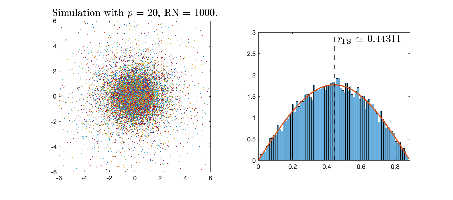
Example 5.24 (The function ).
Following Example 5.19, let us consider the function . The only vanishing point for is (corresponding to ), and the vanishing order is . Since , by Theorem 5.6, the random zeros will converge to as . We shall expect a nice approximation as shown in the right-hand side of Figure 3 for sufficently large .
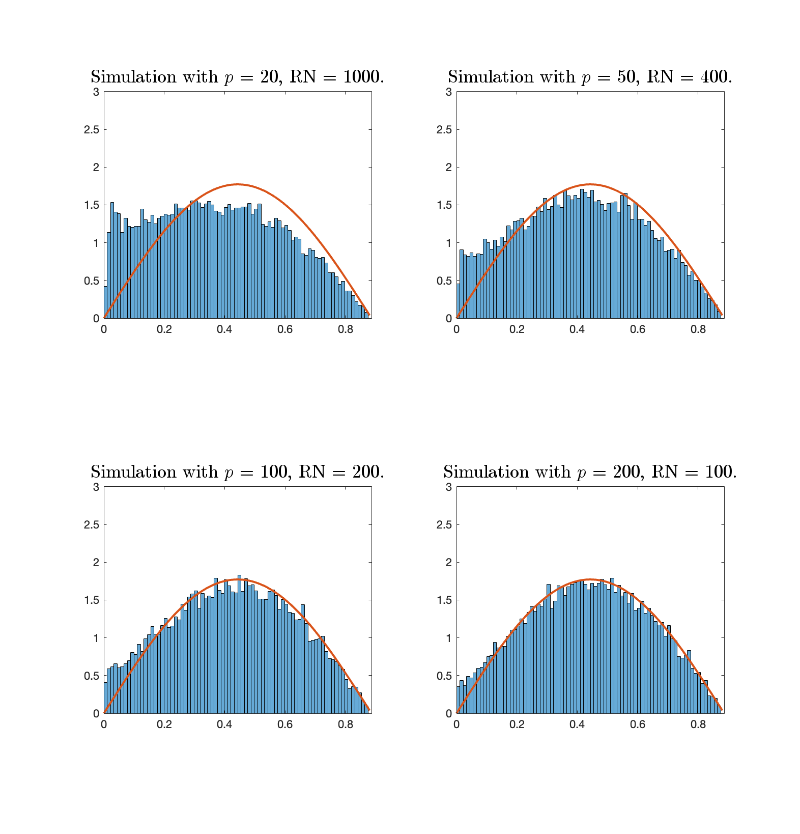
We did simulations for different degrees: . The results are displayed as pictures in Figure 4. It is a straighforward observation that the simulated random zeros approximate better and better to the expected one represented by as the degree grows. This is exactly the main point proved in Theorem 5.6. In the same time, we see also that, different from the case of -polynomial in Figure 3, the result with degree in Figure 4 does not fit nicely with . The main deviation happens around (), which is exactly the unique vanishing point of the function . Roughly speaking, this vanishing point is a sort of global minimizer of on , such that for small , one should observe more zeros around this minimizer.
Example 5.25 (The function ).
A simulation result for the indicator function was shown in Figure 1. As in previous example, we now increase the degrees: in Figure 5, we show how the simulated zeros change as the degree goes from to . As in Theorems 1.12 and 1.16, the random zeros approximate to on the support of (the part ). But outside the support, the simulated zeros do not converge to , and the observation is that the density of random zeros has a rapid drop outside but near the support, and has a concentration near the farthest point from the support. It is an interesting question to investigate such phenomenon in general.
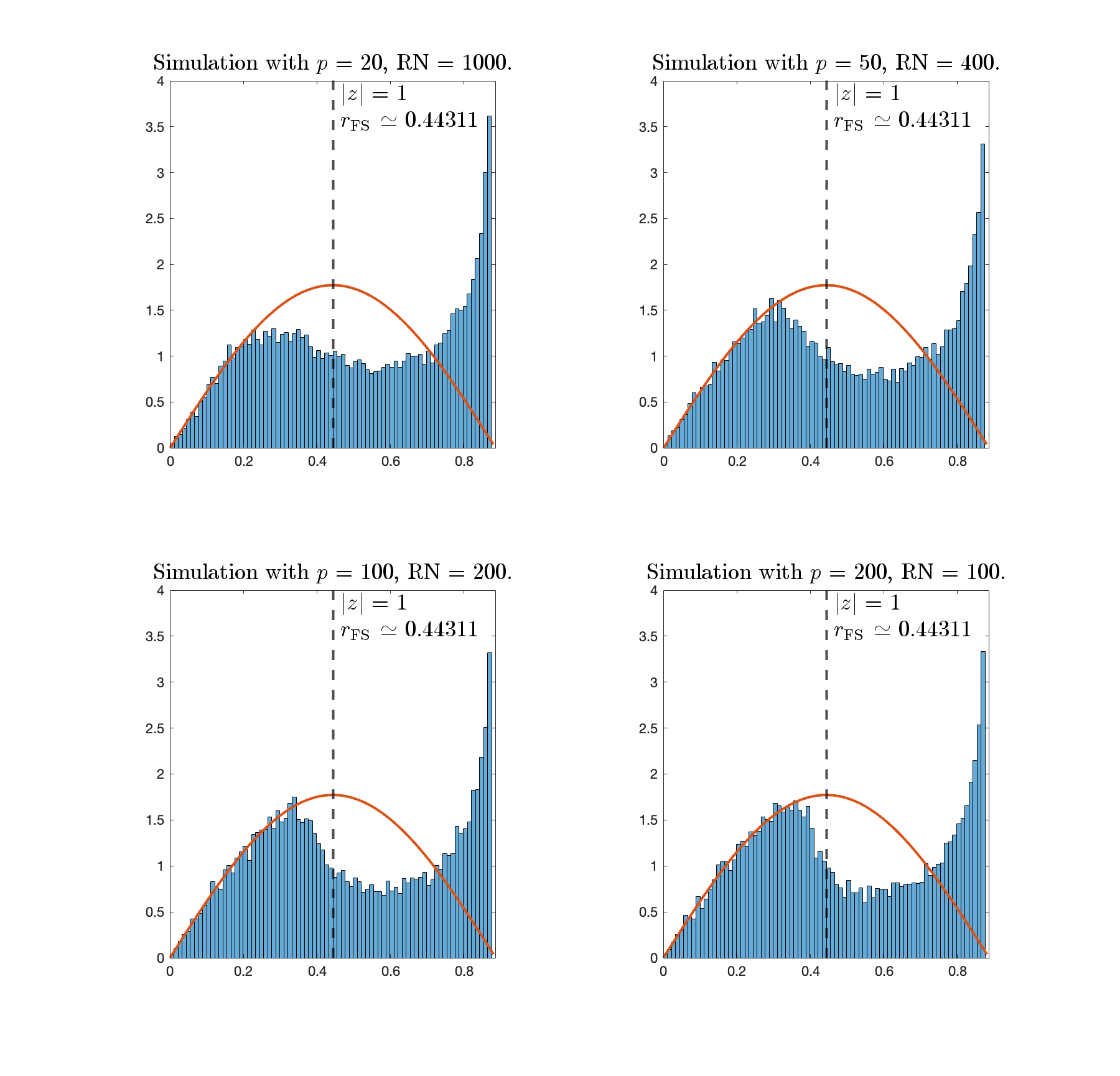
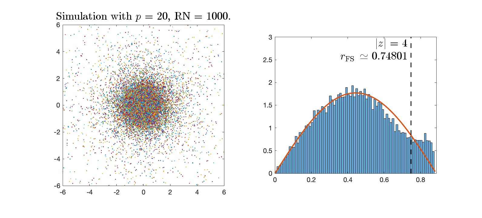
If we increase the radius , that is, enlarging the support of the function to define the Toeplitz operator, we will observe that the simulation of random zeros at degree behaves better than in Figure 1 when we compare it with the density function . In Figure 6, we show a simulation result for and , , and such result is supported by Theorem 1.8 under the condition that the support of nearly fills in the whole part of .
6. Smooth statistics for random zeros of -holomorphic sections
In this section, we always consider the same geometric setting in Sections 2 and 4, in particular, we assume the Condition 1.1 to hold.
We also concentrate on the case and the associated random sections , . The goal of this section is to explain some partial extensions of the seminal results on the smooth statistics of random zeros obtained by Shiffman–Zelditch [49, 50] on compact Kähler manifolds to the zeros of inside the support of . In particular, we focus on the number variance of with a given test form supported in and the corresponding central limit theorem (see also [52]). Note that, except allowing to be noncompact , another difference in our geometric setting from [49, 50] is that we do not assume the connection between the Hermitian form with . The proofs essentially follow from the arguments presented in [49, 50], and we will point out the necessary modifications for our setting.
6.1. Number variance on the support of the symbol
For which is not identically zero, we have studied in Section 5 the random -currents () on , especially, the expectations . Now we are going to study the variance of .
Following [49, §3], we now introduce the variance current of . Let denote the projections to the first and second factors. Then if and are two currents on with respective degree and , then we define a current of degree on as follows
| (6.1) |
In particular, defines a random -current on .
In the same time, we introduce the following notation: for a current on , we write
| (6.2) |
where , denote the corresponding -operators on the first and second factors of . Let be a local complex coordinate on the first factor of , and let be a local complex coordinate on the second factor of , then we can write locally
| (6.3) |
Similarly, we also write .
Definition 6.1.
The variance current of , denoted as , is a -current on defined by
| (6.4) |
In order to simplify the notation, it is enough to consider only the real test forms . For , we have
| (6.5) |
Shiffman and Zelditch [49, 50] established the framework to compute such variance current on a compact Kähler manifold, in particular, they obtained a pluri-bipotential for it. Their method can be easily adapted to our setting. Let us start with recalling the main ingredients from their results.
For , we set the function
| (6.6) |
This is an analytic function with radius of convergence . Moreover, for , we have .
Set . Recall that the function on is defined in (1.39). This is a smooth function on with values in . In particular, for , .
Definition 6.2 (cf. [49, Theorem 3.1]).
For , define
| (6.7) |
Then is a continuous function on .
Since the near-diagonal behavior of depend on if there points lie in the support of or not, which are different from the case for Bergman kernel (such as in [49, 50] or [27, Section 1.5]). Following the computations in [49, §3.1] and we use our results proved in Theorem 1.20 and Lemma 2.13, we have the following results for .
Proposition 6.3 (cf. [49, §3.1]).
Let be an open subset of such that (hence is compact).
-
(i)
Then there exists an integer such that for all , never vanishes on . Moreover, for all , the function is smooth on the region ( denotes the diagonal) and it is on .
-
(ii)
Fix and , then for all sufficiently large and for , with , we have
(6.8) where is defined in (2.12).
-
(iii)
For given , there exist a sufficiently large such that there exist a constant such that for all , , we have
(6.9)
For a real -form on with -coefficients, recall that is defined by
| (6.10) |
Recall also that we have two volume forms and (see (4.72)). Moreover, we have
| (6.11) |
where the positive function on is given in (2.7).
Theorem 6.4.
Let be a connected complex Hermitian manifold and let , be two holomorphic line bundles on with smooth Hermitian metrics. We assume Condition 1.1 (see also (4.1)) to hold. Fix which is not identically zero, and let be an open subset of such that . Then for sufficiently large , we have the identity of -currents on ,
| (6.12) |
Let be a real -form on with -coefficients and , then we have the formula for ,
| (6.13) |
where
Proof.
We sketch the proof based at the proofs of [49, Theorem 3.1] and [50, §3.1]. At first, fix a test form , a routine calculation (see also [26, Proof of Theorem 3.7]) shows that
| (6.14) |
Then by Proposition 6.3 (i) and [49, Lemma 3.3], on and for all , we have
| (6.15) |
where is the Euler’s constant. Then we can rewrite (6.14) as
| (6.16) |
This way, we get (6.12). In fact, (6.16) still holds if is with -coefficients, now we show (6.13) by using Proposition 6.3-(ii) and (iii).
The first step is to rewrite the integral in the form
| (6.17) |
As in [50, §3.1], we set for ,
| (6.18) |
Let be a fixed number which is sufficiently large as in Proposition 6.3 (iii) with . Then we have for ,
| (6.19) |
As in (2.14), let denote the Euclidean volume form on the real vector space . Then for , we have
| (6.20) |
Since is on , then by Proposition 6.3-(ii) and [50, (34)–(37)], we get for a fix small ,
| (6.21) |
By (2.16), we can fix to be large enough such that
| (6.22) |
In the same time, by the formula (2.12) for , then for , we have
| (6.23) |
Finally, combining the Taylor series (6.6) with (6.18) – (6.23), we get for ,
| (6.24) |
after taking the integration with respect to , we conclude exactly (6.13). This way, we complete our proof. ∎
6.2. Asymptotic normality of random zeros; proof of Theorem 1.17
The asymptotic normality of the zeros of random holomorphic functions or sections has been introduced and proved by Sodin–Tsirelson [52] for certain random holomorphic functions on or and by Shiffman–Zelditch [50, Theorem 1.2 and §4] for the random holomorphic sections of line bundles on a compact Kähler manifold. One key ingredient in their approaches is the normalized Bergman kernel which is the covariance function of the corresponding Gaussian holomorphic fields on or , analogous to the construction in the proof of Proposition 4.8. Then the problem is reduced to the seminal result proved by Sodin and Tsirelson in [52, Theorem 2.2] for the non-linear functionals of Gaussian process.
Let us recall the main result of [52, §2.1]. Let be a measure space with a finite positive measure (with ). We also fix a sequence of measurable functions , such that on ,
| (6.25) |
We consider a complex-valued Gaussian process on defined as
| (6.26) |
Then is a sequence of i.i.d. standard complex Gaussian random variables. Then for each , . The covariance function for is given by
| (6.27) |
Let be a sequence of independent Gaussian processes on described as above, and let () denote the corresponding covariance functions. We also fix a nontrivial real function , and a bounded measurable function , set
| (6.28) |
Sodin and Tsirelson proved the following results.
Theorem 6.5 ([52, Theorem 2.2]).
With the above constructions, and suppose that
-
(i)
for if is monotonically increasing, or for all otherwise;
-
(ii)
Then the distributions of the random variables
| (6.29) |
converge weakly to the (real) standard Gaussian distribution as .
Now we are ready to present the proof of Theorem 1.17.
Proof of Theorem 1.17.
The proof is an easy modification of [50, §4 Proof of Theorem 1.2], together with the results in Theorem 1.20 due to the assumption .
We take , , which satisfies the conditions in Theorem 6.5. Let be a continuous section such that on . For each , fix an orthonormal basis consisting of the eigensections of for nonzero eigenvalues . Then on , we write
| (6.30) |
Then we can set , which forms a sequence of measurable functions on satisfying (6.25). Then by (4.27), we have the identity on
| (6.31) |
where is the Gaussian process on constructed as in (6.26). The covariance function for is given by
| (6.32) |
Let be the random variable defined as in (6.28) from . Then (6.31) implies that
| (6.33) |
where is a deterministic constant. Thus the asymptotic normality of is equivalent to that of , which follows by checking the Conditions (i) and (ii) in Theorem 6.5 for . Finally, we apply Theorem 1.20 and proceed as in the last part of [50, §4]. This completes the proof. ∎
Declarations
Conflict of interest. On behalf of all authors, the corresponding author states that there is no conflict of interest.
Data sharing. Data sharing not applicable to this article as no datasets were generated or analyzed during the current study.
References
- [1] M. Ancona and Y. Le Floch, Berezin-Toeplitz operators, Kodaira maps, and random sections, ArXiv:2206.15112, (2022).
- [2] J. r. E. Andersen, Asymptotic faithfulness of the quantum representations of the mapping class groups, Ann. of Math. (2), 163 (2006), pp. 347–368.
- [3] T. Barron, Toeplitz operators on Kähler manifolds, SpringerBriefs in Mathematics, Springer, Cham, 2018.
- [4] T. Barron and D. Itkin, Toeplitz operators with discontinuous symbols on the sphere, in Lie theory and its applications in physics, vol. 191 of Springer Proc. Math. Stat., Springer, Singapore, 2016, pp. 573–581.
- [5] T. Barron, X. Ma, G. Marinescu, and M. Pinsonnault, Semi-classical properties of Berezin-Toeplitz operators with -symbol, J. Math. Phys., 55 (2014), pp. 042108, 25.
- [6] T. Bayraktar, Mass equidistribution for random polynomials, Potential Anal., 53 (2020), pp. 1403–1421.
- [7] B. Berndtsson, Bergman kernels related to Hermitian line bundles over compact complex manifolds, in Explorations in complex and Riemannian geometry, vol. 332 of Contemp. Math., Amer. Math. Soc., Providence, RI, 2003, pp. 1–17.
- [8] J.-M. Bismut, X. Ma, and W. Zhang, Asymptotic torsion and Toeplitz operators, J. Inst. Math. Jussieu, 16 (2017), pp. 223–349.
- [9] P. Bleher, B. Shiffman, and S. Zelditch, Poincaré-Lelong approach to universality and scaling of correlations between zeros, Comm. Math. Phys., 208 (2000), pp. 771–785.
- [10] , Universality and scaling of correlations between zeros on complex manifolds, Invent. Math., 142 (2000), pp. 351–395.
- [11] V. I. Bogachev, Measure theory. Vol. I, II, Springer-Verlag, Berlin, 2007.
- [12] M. Bordemann, E. Meinrenken, and M. Schlichenmaier, Toeplitz quantization of Kähler manifolds and , limits, Comm. Math. Phys., 165 (1994), pp. 281–296.
- [13] L. Charles and B. Estienne, Entanglement entropy and Berezin-Toeplitz operators, Comm. Math. Phys., 376 (2020), pp. 521–554.
- [14] L. Charles and L. Polterovich, Sharp correspondence principle and quantum measurements, Algebra i Analiz, 29 (2017), pp. 237–278.
- [15] M. Christ, Slow off-diagonal decay for Szegö kernels associated to smooth Hermitian line bundles, in Harmonic analysis at Mount Holyoke (South Hadley, MA, 2001), vol. 320 of Contemp. Math., Amer. Math. Soc., Providence, RI, 2003, pp. 77–89.
- [16] , Off-diagonal decay of Bergman kernels: on a question of Zelditch, in Algebraic and analytic microlocal analysis, vol. 269 of Springer Proc. Math. Stat., Springer, Cham, 2018, pp. 459–481.
- [17] , Upper bounds for Bergman kernels associated to positive line bundles with smooth Hermitian metrics, in Algebraic and analytic microlocal analysis, vol. 269 of Springer Proc. Math. Stat., Springer, Cham, 2018, pp. 437–457.
- [18] D. Coman and G. Marinescu, Equidistribution results for singular metrics on line bundles, Ann. Sci. Éc. Norm. Supér. (4), 48 (2015), pp. 497–536.
- [19] S. Csörgő, K. Tandori, and V. Totik, On the strong law of large numbers for pairwise independent random variables, Acta Math. Hungar., 42 (1983), pp. 319–330.
- [20] G. de Rham, Variétés différentiables. Formes, courants, formes harmoniques, Publications de l’Institut de Mathématique de l’Université de Nancago, III, Hermann, Paris, 1973. Troisième édition revue et augmentée, Actualités Scientifiques et Industrielles [Current Scientific and Industrial Topics], No. 1222b.
- [21] A. Deleporte, Low-energy spectrum of Toeplitz operators: the case of wells, J. Spectr. Theory, 9 (2019), pp. 79–125.
- [22] , Low-energy spectrum of Toeplitz operators with a miniwell, Comm. Math. Phys., 378 (2020), pp. 1587–1647.
- [23] , Toeplitz operators with analytic symbols, J. Geom. Anal., 31 (2021), pp. 3915–3967.
- [24] H. Delin, Pointwise estimates for the weighted Bergman projection kernel in , using a weighted estimate for the equation, Ann. Inst. Fourier (Grenoble), 48 (1998), pp. 967–997.
- [25] J.-P. Demailly, Complex Analytic and Differential Geometry, 2012. Published online at https://www-fourier.ujf-grenoble.fr/~demailly/documents.html.
- [26] A. Drewitz, B. Liu, and G. Marinescu, Gaussian holomorphic sections on noncompact complex manifolds, ArXiv:2302.08426, (2023).
- [27] , Large deviations for zeros of holomorphic sections on punctured riemann surfaces, Michigan Mathematical Journal, Advance Publication (2023), pp. 1–41.
- [28] H. Federer, Geometric measure theory, Die Grundlehren der mathematischen Wissenschaften, Band 153, Springer-Verlag New York, Inc., New York, 1969.
- [29] Y. L. Floch, A Brief Introduction to Berezin–Toeplitz Operators on Compact Kähler Manifolds, Springer International Publishing, 2018.
- [30] P. Griffiths and J. Harris, Principles of algebraic geometry, Wiley Classics Library, John Wiley & Sons, Inc., New York, 1994.
- [31] L. Gross, Abstract Wiener spaces, in Proc. Fifth Berkeley Sympos. Math. Statist. and Probability (Berkeley, Calif., 1965/66), Vol. II: Contributions to Probability Theory, Part 1, Univ. California Press, Berkeley, Calif., 1967, pp. 31–42.
- [32] J. H. Hannay, Chaotic analytic zero points: exact statistics for those of a random spin state, J. Phys. A, 29 (1996), pp. L101–L105.
- [33] L. Hörmander, Notions of convexity, vol. 127 of Progress in Mathematics, Birkhäuser Boston, Inc., Boston, MA, 1994.
- [34] R. A. Horn and C. R. Johnson, Matrix analysis, Cambridge University Press, Cambridge, 1985.
- [35] L. Ioos, W. Lu, X. Ma, and G. Marinescu, Berezin-Toeplitz quantization of non-compact manifolds, In preparation.
- [36] C. I. Lazaroiu, D. McNamee, and C. Sämann, Generalized Berezin quantization, Bergman metrics and fuzzy Laplacians, J. High Energy Phys., (2008), pp. 059, 60.
- [37] N. Lindholm, Sampling in weighted spaces of entire functions in and estimates of the Bergman kernel, J. Funct. Anal., 182 (2001), pp. 390–426.
- [38] Z. Lu and S. Zelditch, Szegő kernels and Poincaré series, J. Anal. Math., 130 (2016), pp. 167–184.
- [39] X. Ma and G. Marinescu, Holomorphic Morse inequalities and Bergman kernels, vol. 254 of Progress in Mathematics, Birkhäuser Verlag, Basel, 2007.
- [40] , Toeplitz operators on symplectic manifolds, J. Geom. Anal., 18 (2008), pp. 565–611.
- [41] , Berezin-Toeplitz quantization on Kähler manifolds, J. Reine Angew. Math., 662 (2012), pp. 1–56.
- [42] , Exponential estimate for the asymptotics of Bergman kernels, Math. Ann., 362 (2015), pp. 1327–1347.
- [43] S. Nonnenmacher and A. Voros, Chaotic eigenfunctions in phase space, J. Statist. Phys., 92 (1998), pp. 431–518.
- [44] J. P. Oldfield, Two-term Szegő theorem for generalised anti-Wick operators, J. Spectr. Theory, 5 (2015), pp. 751–781.
- [45] L. Polterovich, Symplectic rigidity and quantum mechanics, in European Congress of Mathematics, Eur. Math. Soc., Zürich, 2018, pp. 155–179.
- [46] O. Rouby, J. Sjöstrand, and S. V. u. Ngọc, Analytic Bergman operators in the semiclassical limit, Duke Math. J., 169 (2020), pp. 3033–3097.
- [47] M. Schlichenmaier, Berezin-Toeplitz quantization and Berezin transform, in Long time behaviour of classical and quantum systems (Bologna, 1999), vol. 1 of Ser. Concr. Appl. Math., World Sci. Publ., River Edge, NJ, 2001, pp. 271–287.
- [48] B. Shiffman and S. Zelditch, Distribution of zeros of random and quantum chaotic sections of positive line bundles, Comm. Math. Phys., 200 (1999), pp. 661–683.
- [49] , Number variance of random zeros on complex manifolds, Geom. Funct. Anal., 18 (2008), pp. 1422–1475.
- [50] , Number variance of random zeros on complex manifolds, II: smooth statistics, Pure Appl. Math. Q., 6 (2010), pp. 1145–1167.
- [51] B. Shiffman, S. Zelditch, and S. Zrebiec, Overcrowding and hole probabilities for random zeros on complex manifolds, Indiana Univ. Math. J., 57 (2008), pp. 1977–1997.
- [52] M. Sodin and B. Tsirelson, Random complex zeroes. I. Asymptotic normality, Israel J. Math., 144 (2004), pp. 125–149.
- [53] T. Tao and V. Vu, Local universality of zeroes of random polynomials, Int. Math. Res. Not. IMRN, (2015), pp. 5053–5139.
- [54] S. Zelditch, Quantum ergodic sequences and equilibrium measures, Constr. Approx., 47 (2018), pp. 89–118.