SPHINCS_BSSN: Numerical Relativity with Particles

Abstract

In this chapter we describe the Lagrangian numerical relativity code SPHINCS_BSSN. This code evolves spacetimes in full General Relativity by integrating the BSSN equations on structured meshes with a simple dynamical mesh refinement strategy. The fluid is evolved by means of freely moving Lagrangian particles, that are evolved using a modern Smooth Particle Hydrodynamics (SPH) formulation. To robustly and accurately capture shocks, our code uses artificial dissipation terms, but, similar to Finite Volume schemes, we apply a slope-limited reconstruction within the dissipative terms and we use in addition time-dependent dissipation parameters, so that dissipation is only applied where needed. The technically most complicated, but absolutely crucial part of the methodology, is the coupling between the particles and the mesh. For the mapping of the energy-momentum tensor $T_{\mu\nu}$ from the particles to the mesh, we use a sophisticated combination of ”Local Regression Estimate” (LRE) method and a ”multi-dimensional optimal order detection” (MOOD) approach which we describe in some detail. The mapping of the metric quantities from the grid to the particles is achieved by a quintic Hermite interpolation.
Apart from giving an introduction to our numerical methods, we demonstrate the accurate working of our code by presenting a set of representative relativistic hydrodynamics tests. We begin with a relativistic shock tube test, then compare the frequencies of a fully relativistic neutron star with reference values from the literature and, finally, we present full-blown merger simulations of irrotational binary systems, one case where a central remnant survives and another where a black hole forms, and of a binary where only one of the stars is rapidly spinning.

0.1 Introduction

Despite their early postulation by Albert Einstein in 1916 Einstein (1916, 1918), gravitational waves (GWs) remained a topic of sustained debate for more than half a century Kennefick (2007). Their physical reality was only firmly established after the discovery of the Hulse-Taylor pulsar in 1974 Hulse and Taylor (1975): the secular orbital decay of this neutron star binary system is in nearly perfect agreement with the prediction from Einstein’s theory and this finally brought the decades’ long controversy to an end. Still, the first direct detection of GWs had to wait until 2015 when both LIGO detectors recorded the last 0.2 seconds of the inspiral and the subsequent merger of two $\sim 30$ M_⊙ black holes Abbott et al. (2016).
The first detection of a GW source that actually involved matter (rather than ”just black holes”), followed soon: in August 2017 a $\sim$ minute-long GW-signal from a merging neutron star binary (GW170817) was detected. Most excitingly, this event was also observed in electromagnetic (EM) waves, first as a short gamma-ray burst (GRB) that followed the peak of the GW emission with a delay of 1.7 s, later ($\sim$ days) as a radioactively powered thermal transient peaking at optical/near-infrared wavelengths frequently called a ”kilonova”, and much later ($\sim$ months) also in radio wavelengths, see Margutti and Chornock (2021) for a recent review.
This event meant a huge leap forward for many long-standing (astro-)physics questions. For example, the electromagnetic follow-up observations of GW170817 revealed the actual host galaxy where the merger took place and this placed the event in an astronomical environment and connected it to potential stellar evolution paths Levan et al. (2017). Since the distance to the host galaxy is known, it was possible to use the 1.7 s delay between GWs and the GRB to show that GWs propagate to a relative accuracy of $10^{-15}$ at the speed of light Abbott et al. (2017a). This, in turn, eliminated families of alternative theories of gravity where $c_{\rm GW}\neq c$. GW170817 also demonstrated the exciting possibility to constrain the properties of cold nuclear matter via the effects of tidal deformability and thereby ruled out some very stiff equations of state Abbott et al. (2017b). The event further showed that neutron star mergers are, as expected on theoretical grounds Lattimer et al. (1977); Symbalisty and Schramm (1982); Eichler et al. (1989); Rosswog et al. (1999); Freiburghaus, Rosswog, and Thielemann (1999), major cosmic production sites of heavy ”r-process” elements Cowan et al. (2021), and that they are useful probes of the cosmic expansion Abbott et al. (2017c).
All of these breakthroughs were enabled by the combined detection of the same event via different messengers, here GWs and photons. This detection splendidly illustrated the huge discovery potential of multi-messenger astrophysics, but it also underlined the enormous modelling challenge: in addition to strong-field gravity, relativistic fluid dynamics, neutrino transport, magnetic fields, nuclear reactions and atomic physics, also (non-equilibrium) radiative transfer should be included in theoretical models in order to make the connection to the EM observations.

Numerical simulations, especially numerical relativity simulations Alcubierre (2008); Baumgarte and Shapiro (2010); Rezzolla and Zanotti (2013); Shibata (2016), play a very crucial role in connecting the physical processes during merger to potentially observable signals. Such simulations have increasingly become tools for exploring signatures from both established and more speculative parts of fundamental physics. Multi-physics numerical relativity simulations are extremely complex and time consuming: codes typically evolve several dozen variables per spacetime (grid-) point and, depending on the simulated physics, many more variables may be needed. For example, neutrino transport is needed to make detailed predictions for the neutron-to-proton-ratio in the ejecta, which, in turn, determines which elements are formed and therefore also how the electromagnetic signal looks like. But evolving several neutrino flavours, with many energy groups for each of them, becomes a serious extra computational burden Mezzacappa et al. (2020); Radice et al. (2022); Foucart (2023). To make things worse, the spacetime needs to be evolved with very small numerical time steps that are limited by the Courant criterion Press et al. (1992). The ”signal speed” that enters this criterion is the speed of light, which limits the admissible time steps to $\Delta_{t}\approx 10^{-7}\;s\;\left(\frac{\Delta x}{100\rm m}\right)$, where $\Delta x$ is the spatial length to be resolved.

To date, essentially all numerical relativity codes that solve the full set of Einstein equations are Eulerian, i.e. they solve the fluid equations on computational (usually structured or adaptive) grids. The only exception is our code SPHINCS_BSSN Rosswog and Diener (2021); Diener, Rosswog, and Torsello (2022); Rosswog, Diener, and Torsello (2022); Rosswog, Torsello, and Diener (2023), which is the main topic of this book chapter. Using an alternative methodology makes it possible to independently cross-validate the longer established Eulerian methods, but it also comes with distinctive advantages for multi-messenger astrophysics. One of its salient features is that –contrary to Eulerian methods– vacuum does not need to be modelled hydrodynamically: it is simply characterized by the absence of computational elements (here: particles) and no computational resources need to be spent to evolve it. Moreover, the neutron star surface, which is an eternal source of numerical trouble for Eulerian methods, is very well-behaved and does not need any particular treatment compared to the rest of the fluid. The ejecta of a neutron star merger correspond to only $\sim$ 1% of the binary mass, but they are responsible for essentially all of the EM emission. Therefore, the accurate prediction of the properties of this small amount of matter is of paramount importance for multi-messenger astrophysics. This is, in fact, one of the key strengths of a code like SPHINCS_BSSN: advection is exact (i.e. not depending on the resolution) and the properties of a particle, say its electron fraction $Y_{e}$, are simply transported by the particle unless they are changed by physical processes (e.g. by an electron capture reaction), but no purely numerical ”diffusive” processes occur.

In the rest of this chapter, we will describe the methodology behind our Lagrangian Numerical Relativity code SPHINCS_BSSN and we will present some of the first applications. In Sec. 0.2 we will describe how we evolve fluids and, since in a numerical relativity context the use of particles is not widespread, we start with some basics of the SPH method. We further outline how the spacetime is evolved and how the fluid particles and the grid cells for the spacetime evolution exchange information. In Sec. 0.3 we will show some applications of the code including some standard benchmark tests, but also some of the first astrophysical simulations. We finally will summarize this chapter in Sec. 0.4.

0.2 Methodology

Here we will briefly summarize the main methodological elements that enter in SPHINCS_BSSN. We will focus here on the main ideas and in some cases we will refer to our more technical papers Rosswog and Diener (2021); Diener, Rosswog, and Torsello (2022); Rosswog, Diener, and Torsello (2022); Rosswog, Torsello, and Diener (2023) for the full details.

0.2.1 Relativistic Smooth Particle Hydrodynamics

Our main aim here is to describe how we evolve matter by means of a modern, general relativistic Smooth Particle Hydrodynamics (SPH) code. But before we do so, we will summarize some basic SPH techniques and we will briefly discuss the (simpler to understand) Newtonian SPH approach. Once equipped with this basic knowledge, the general relativistic version should be straight forward to grasp.
This introduction to the topic is by no means meant as a comprehensive SPH review, for a more complete introduction to the SPH-method, its variants and subtleties and its various applications in astrophysics and cosmology, we refer to extensive reviews that exist in the literature Monaghan (1992, 2005); Rosswog (2009); Springel (2010a); Price (2012); Rosswog (2015a, b). For relativistic formulations of SPH, we specifically want to point to Laguna, Miller, and Zurek (1993); Siegler and Riffert (2000); Monaghan and Price (2001); Rosswog (2009, 2010a, 2010b, 2011); Rosswog and Diener (2021); Diener, Rosswog, and Torsello (2022); Rosswog, Diener, and Torsello (2022); Rosswog, Torsello, and Diener (2023). Among these, we will frequently refer to Rosswog (2009) since here many results are derived very explicitly in a step-by-step fashion.

A primer on basic SPH-techniques

The main idea of SPH is to model a fluid via spherical particles of finite size and overlapping support. These particles move with the local fluid velocity, i.e. SPH is a fully Lagrangian method, as opposed to Eulerian or Adaptive Lagrangian Eulerian, or ”ALE”, methodologies. The overlapping nature of the particles distinguishes them, for example, from (usually quasi-) Lagrangian Moving Mesh methods, see e.g. Springel (2010b); Duffell and MacFadyen (2011), which instead tessellate space into non-overlapping cells which have a sharp interface surface between them. The task is now to translate the continuum equations of Lagrangian fluid dynamics into evolution equations for the particles, ideally in a way that ensures that nature’s conservation laws are enforced on the level of the particle evolution equations. In the simplest case of ideal, non-relativistic fluids the equations read

$$\frac{d\rho}{dt} = -\rho\nabla\cdot\vec{v}$$ (1)

$$\frac{d\vec{v}}{dt} = -\frac{\nabla P}{\rho}+\vec{f}$$ (2)

$$\frac{du}{dt} = \frac{dq}{dt}+\frac{P}{\rho^{2}}\frac{d\rho}{dt}.$$ (3)

Here, $\rho$ is the mass density, $\vec{v}$ the fluid velocity, $P$ the pressure, $\vec{f}$ denote other ”body forces” e.g. from gravity, $u$ is the specific internal energy (i.e. energy per mass) and $dq/dt$ denotes potential sources of heating and/or cooling. The Lagrangian time derivative, $d/dt$, is related to the Eulerian time derivative $\partial/\partial t$ by

$$\frac{d}{dt}(.)=\left(\frac{\partial}{\partial t}+\vec{v}\cdot\nabla\right)(.).$$ (4)

Note that Eq. (3) is simply the first law of thermodynamics written ”on a per mass basis”, i.e. the involved quantities are e.g. energy per mass or volume per mass (=1/density).
At the heart of the SPH method is kernel interpolation. Assuming that some quantity $f$ is known at particle location $b$, a smoothed version of the quantity $\langle f\rangle$ reads

$$\langle f\rangle(\vec{r})=\int f(\vec{r^{\prime}})\;W_{h}(\vec{r}^{\prime}-\vec{r})\;d^{3}x^{\prime}\approx\sum_{b}V_{b}f_{b}W_{h}(\vec{r_{b}}-\vec{r})=\sum_{b}\frac{m_{b}}{\rho_{b}}\;f_{b}\;W_{h}(\vec{r_{b}}-\vec{r}).$$ (5)

Here $W_{h}$ is a smoothing kernel, see below, whose support size is determined by the length scale $h$, which, in an SPH context, is usually referred to as the “smoothing length”. In the approximation we have applied a one-point quadrature. In SPH, one usually chooses the particle volume as $m_{b}/\rho_{b}$, where $m_{b}$ and $\rho_{b}$ are the particle mass and mass density at the position of particle $b$, but other choices are possible, see e.g. Hopkins (2013); Rosswog (2015a); Cabezon, Garcia-Senz, and Figueira (2017) for alternatives. One simple application of Eq. (5) is to choose the density $\rho$ for the quantity $f$, which yields

$$\langle\rho\rangle_{a}=\sum_{b}m_{b}W_{ab}(h_{a}),$$ (6)

where $W_{ab}(h_{a})$ is a short-hand for $W((\vec{r}_{a}-\vec{r}_{b})/h_{a})$. In other words: the density can be calculated by summing over the local neighbourhood and weighting each particle’s mass according to how far away it is from particle $a$. If one keeps each particle’s mass fixed in time, one has enforced exact mass conservation and one does not have to solve the mass conservation equation (1) explicitly, but one can do so if this is desired.
Clearly, for the smoothing procedure in Eq. (5) to make sense, the smoothing kernel must have certain properties:

• it needs to be normalized, $\int W_{h}(\vec{r}^{\prime})d^{3}r^{\prime}=1$,

• obviously, the dimension of the kernel has to be “1/volume”,

• it has to have the “delta-property”, so as to reproduce the original function in the limit of vanishing support size,

  $$\lim_{h\rightarrow 0}\int W_{h}(\vec{r}^{\prime}-\vec{r})\;f(r^{\prime})\;d^{3}r^{\prime}=f(r)$$ (7)

• and it should (at least) have a continuous second derivative.

A number of other properties are desirable, for example, the kernel should be ”radial”, i.e. $W_{h}(\vec{x}-\vec{x}^{\prime})=W_{h}(|\vec{x}-\vec{x}^{\prime})|)$, to easily allow for the conservation of momentum and angular momentum, and its Fourier transform should fall of rapidly with wave number (Monaghan, 1985). As a side remark: it may seem appealing to use an oblate kernel to model, say, an accretion disk, but this approach would sacrifice one of SPH’s most salient features: its exact angular momentum conservation. The latter can be easily enforced when radial kernel are used, see Sec. 2.4 in Rosswog (2009) for an explicit demonstration how radial kernels lead to exact angular momentum conservation.
For a gradient estimate, one can straight forwardly apply the nabla operator to Eq. (5)

$$\nabla f(\vec{r})=\sum_{b}\frac{m_{b}}{\rho_{b}}\;f_{b}\;\nabla_{r}W_{h}(\vec{r_{b}}-\vec{r}),$$ (8)

where the index $r$ at the nabla operator indicates that the derivative is taken with respect to the variable $\vec{r}$ (rather than $\vec{r}_{b}$). The derivatives are usually needed at the position of a particle (here labelled $a$) and abbreviated as

$$(\nabla f)_{a}=\sum_{b}\frac{m_{b}}{\rho_{b}}f_{b}\nabla_{a}W_{ab}(h_{a}),$$ (9)

where the label at the nabla operator is again a reminder that the derivative is taken with respect to $\vec{r}_{a}$ (and not $\vec{r}_{b}$). From Eq. (5) it is obvious that one would want to have the “partition of unity” property in a discrete form at any position $\vec{r}$

$$1 = \sum_{b}\frac{m_{b}}{\rho_{b}}\;W_{h}(\vec{r_{b}}-\vec{r})$$ (10)

$$0 = \nabla_{r}(1)=\sum_{b}\frac{m_{b}}{\rho_{b}}\;\nabla_{r}W_{h}(\vec{r_{b}}-\vec{r}),$$ (11)

where the second equation is simply the result of applying the nabla operator to the first one. In standard SPH these equations are only approximately fulfilled and the accuracy depends on the kernel function used, its support size (or the number of contributing particles) and on the exact particle distribution. This has the effect, that when applying Eq. (8) to a constant function $f=f_{0}$, one only approximately recovers the theoretical value of zero

$$\nabla_{r}\left(\sum_{b}\frac{m_{b}}{\rho_{b}}f_{b}W_{h}(\vec{r_{b}}-\vec{r})\right)=f_{0}\sum_{b}\frac{m_{b}}{\rho_{b}}\nabla_{r}W_{h}(\vec{r_{b}}-\vec{r})\approx 0.$$ (12)

This, however, can be easily corrected by simply “subtracting a numerical zero”, so that a better gradient estimate reads

$$\left(\nabla f\right)^{(1)}_{a} =\sum_{b}\frac{m_{b}}{\rho_{b}}f_{b}\nabla_{a}W_{ab}(h_{a})-\left(f_{a}\sum_{b}\frac{m_{b}}{\rho_{b}}\nabla_{a}W_{ab}(h_{a})\right)$$

$$=\sum_{b}\frac{m_{b}}{\rho_{b}}(f_{b}-f_{a})\nabla_{a}W_{ab}(h_{a}),$$ (13)

and this expression vanishes by construction when all $f_{k}$ are the same. As an example, we can apply this gradient prescription to find an estimate for the velocity divergence. This quantity plays an important role in fluid dynamics, since $\nabla\cdot\vec{v}=0$ defines “incompressibility”, while $\nabla\cdot\vec{v}>0$ indicates local expansion and $\nabla\cdot\vec{v}<0$ means local compression of the fluid. The resulting expression is

$$(\nabla\cdot\vec{v})_{a}=\sum_{b}\frac{m_{b}}{\rho_{b}}(\vec{v}_{b}-\vec{v}_{a})\cdot\nabla_{a}W_{ab}(h_{a}).$$ (14)

An alternative discretization can be found by taking Eq. (1) and calculating the Lagrangian time derivative of Eq. (6) directly

$$(\nabla\cdot\vec{v})_{a}=-\frac{1}{\rho_{a}}\frac{d\rho_{a}}{dt}=-\frac{1}{\rho_{a}}\sum_{b}m_{b}\frac{dW_{ab}}{dt}=\frac{1}{\rho_{a}}\sum_{b}m_{b}(\vec{v}_{b}-\vec{v}_{a})\cdot\nabla_{a}W_{ab}(h_{a}),$$ (15)

where we have taken the straight-forward Lagrangian time derivative of the kernel function (see the kernel table in Sec. 2.3 in Rosswog (2009) where this is shown explicitly). Thus, we have derived an alternative numerical discretization for $\nabla\cdot\vec{v}$, where the difference between the two estimates is whether the local density (”$\rho_{a}$”) or the weighted nearby densities (”$\rho_{b}$”) are used. Both are equally valid and both vanish for the uniform velocity case.
For easy later reference, we explicitly write down once more the Lagrangian time derivative of the density in Eq. (6) that we have just found

$$\frac{d\rho_{a}}{dt}=\sum_{b}m_{b}\frac{d}{dt}\left[W_{ab}(h_{a})\right]=\sum_{b}m_{b}(\vec{v}_{a}-\vec{v}_{b})\cdot\nabla_{a}W_{ab}(h_{a})$$ (16)

and we also note that

$$\nabla_{a}\rho_{b}=\sum_{k}m_{k}\nabla_{a}W_{bk}(h_{b})$$ (17)

(the detailed steps can be found in Sec. 3.2 of Rosswog (2009)). Note that we have neglected small terms, usually called ”grad-h” terms, that result from taking derivatives of the kernel with respect to the smoothing lengths. These terms have been derived for Newtonian hydrodynamics by Springel and Hernquist (2002); Monaghan (2002), for special-relativistic SPH in Rosswog (2010b) and for the General Relativistic case in Rosswog (2010a). We had explored the effects of these grad-h terms in Rosswog and Price (2007), but found them to be too close to unity to warrant the extra effort of an additional iteration ($\rho$ depends on $h$ and $h$ depends on $\rho$, so one needs an iteration for consistent values). Therefore, we will ignore these ”grad-h”-terms for the rest of this chapter.

Newtonian SPH

We have already seen in Eq. (6) that the continuity equation does not need to be solved explicitly, and if we keep the particle masses fixed, we have enforced exact mass conservation. It now turns out that by insightful choices (see the discussion in Sec. 2.3 - 2.5 in Rosswog (2009)), one can also bring the energy and momentum equation into discrete forms so that they conserve the total energy and momentum exactly. If a radial kernel is used, then the total angular momentum is conserved exactly by construction as well. Keep in mind that this exact conservation even holds at finite resolution, which is not the case for Eulerian methods. Moving-mesh methods, see e.g. Springel (2010b); Duffell and MacFadyen (2011), usually show good overall conservation, but angular momentum is not conserved exactly.
One can, however, also achieve exact conservation in a more elegant way: by starting from a Lagrangian and by applying a variational principle (Gingold and Monaghan, 1982; Speith, 1998; Monaghan and Price, 2001; Springel and Hernquist, 2002; Rosswog, 2009; Price, 2012) one finds a fully conservative discrete form of the equations without ambiguities.
As before, we will start here with the simplest case of ideal, Newtonian hydrodynamics, but one can adhere to this strategy also for cases with additional physics, e.g. gravity (Price and Monaghan, 2007). One can start from a discretized Lagrangian of an ideal fluid

$$L=\sum_{b}m_{b}\left(\frac{v_{b}^{2}}{2}-u_{b}\right)$$ (18)

and apply the Euler-Lagrange equations

$$\frac{d}{dt}\frac{\partial L}{\partial\vec{v}_{a}}-\frac{\partial L}{\partial\vec{r}_{a}}=0$$ (19)

to find the momentum evolution equation of each particle, where $\partial L/\partial\vec{v}_{a}$ is the canonical momentum, which for Eq. (18) simply becomes $m_{a}\vec{v}_{a}$. We can use again fixed particle masses and the adiabatic first law of thermodynamics, $du=-Pd(1/\rho)$, which yields

$$\left(\frac{\partial u}{\partial\rho}\right)_{s}=\frac{P}{\rho^{2}},$$ (20)

where $s$ denotes the specific entropy. This yields

$$\frac{d\vec{v}_{a}}{dt} = \frac{1}{m_{a}}\frac{\partial L}{\partial\vec{r}_{a}}=-\frac{1}{m_{a}}\sum_{b}m_{b}\frac{\partial u_{b}}{\partial\rho_{b}}\frac{\partial\rho_{b}}{\partial\vec{r}_{a}}=-\frac{1}{m_{a}}\sum_{b}m_{b}\frac{P_{b}}{\rho_{b}^{2}}\left[\sum_{k}m_{k}\nabla_{a}W_{bk}(h_{b})\right]$$ (21)

$$= -\sum_{b}m_{b}\left(\frac{P_{a}}{\rho_{a}^{2}}\nabla_{a}W_{ab}(h_{a})+\frac{P_{b}}{\rho_{b}^{2}}\nabla_{a}W_{ab}(h_{b})\right),$$

where we have used $\nabla_{a}W_{bk}=\nabla_{b}W_{kb}(\delta_{ba}-\delta_{ka})$, see Sec. 2.3 in Rosswog (2009). For the energy equation, a straight forward insertion of Eq. (15) into Eq. (3) (without the heating/cooling term) yields

$$\frac{du_{a}}{dt}=\frac{P_{a}}{\rho_{a}^{2}}\sum_{b}m_{b}(\vec{v}_{b}-\vec{v}_{a})\nabla_{a}W_{ab}(h_{a}),$$ (22)

and with Eqs. (6), (21) and (22) we now have a complete set of discrete hydrodynamics equations. For practical simulations one would still need to choose an equation of state so that one can calculate pressures and one has to add dissipative mechanisms, e.g. a Riemann solver or artificial viscosity, so that shocks can be handled robustly.

General relativistic SPH

Special- and general-relativistic versions of SPH can be derived similarly to the Newtonian case Monaghan and Price (2001); Rosswog (2009, 2010b, 2010a). We use geometric units with $G=c=1$ and adopt (-,+,+,+) for the metric signature of the metric. We reserve greek letters for space-time indices from 0…3 with 0 being the temporal component and we use $i$ and $j$ for spatial components and SPH particles are labeled by $a,b$ and $k$. Contravariant spatial indices of a vector quantity $\vec{V}$ at particle $a$ are denoted as $V^{i}_{a}$, while covariant ones will be written as $(V_{i})_{a}$. The line element and proper time are given by $ds^{2}=g_{\mu\nu}\;dx^{\mu}\;dx^{\nu}$ and $d\tau^{2}=-ds^{2}$ and the proper time is related to the coordinate time $t$ by

$$\Theta d\tau=dt,$$ (23)

where we have introduced a generalization of the Lorentz-factor

$$\Theta\equiv\frac{1}{\sqrt{-g_{\mu\nu}v^{\mu}v^{\nu}}}.$$ (24)

The coordinate velocity components are given by

$$v^{\mu}=\frac{dx^{\mu}}{dt}=\frac{dx^{\mu}}{d\tau}\frac{d\tau}{dt}=\frac{U^{\mu}}{\Theta}=\frac{U^{\mu}}{U^{0}},$$ (25)

where we have used Eq. (23) and $U^{\mu}$ is the four-velocity which is normalized,

$$U^{\mu}U_{\mu}=-1.$$ (26)

The Lagrangian of a relativistic fluid is given by Fock (1964)

$$L=-\int T^{\mu\nu}U_{\mu}U_{\nu}\sqrt{-g}dV,$$ (27)

where $g={\rm det}(g_{\mu\nu})$ and $T^{\mu\nu}$ denotes the energy-momentum tensor which, for an ideal fluid, reads

$$T^{\mu\nu}=(\tilde{\rho}+P)U^{\mu}U^{\nu}+Pg^{\mu\nu}.$$ (28)

Here $\tilde{\rho}$ is the energy density measured in the local rest frame of the fluid and $P$ is its pressure. For clarity, we will write out explicit factors of $c$ in the following lines. The energy density possesses a contribution from the rest mass and one from the thermal energy:

$$\tilde{\rho}=\rho+u\rho/c^{2}=nm_{0}c^{2}(1+u/c^{2}).$$ (29)

Here $n$ is the baryon number density in the local fluid rest frame, $m_{0}$ is the baryon mass and $u=u(n,s)$ the specific energy, with $s$ being the specific entropy. In SPHINCS_BSSN we measure all energies in units of $m_{0}c^{2}$. With this convention (and now using again $c=1$) the energy momentum tensor reads

$$T^{\mu\nu}=\left\{n(1+u)+P\right\}U^{\mu}U^{\nu}+Pg^{\mu\nu}.$$ (30)

To perform practical simulations, we give up general covariance and choose a particular frame (’computing frame’) in which the simulations are performed. Like in special-relativistic hydrodynamics, one must clearly distinguish between quantities that are measured in the computing frame and those measured in the local rest frame of the fluid. With the normalization of the four-velocity, Eq. (26), the Lagrangian can be written as

$$L=-\int n(1+u)\sqrt{-g}dV.$$ (31)

Local baryon number conservation, $(U^{\mu}n);_{\mu}=0$, can be expressed as

$$\frac{1}{\sqrt{-g}}\partial_{\mu}(\sqrt{-g}U^{\mu}n)=0,$$ (32)

where we have used an identity for the covariant derivative Schutz (1989). More explicitly, we can write

$$\partial_{t}(N)+\partial_{i}(Nv^{i})=0,$$ (33)

where we have made use of Eq. (25) and have introduced the computing frame baryon number density

$$N=\sqrt{-g}\Theta n.$$ (34)

In the special relativistic limit $g_{\mu\nu}\rightarrow\eta_{\mu\nu}$ (Minkowski), $\Theta$ reduces to the special relativistic Lorentz factor $\gamma$ and $\sqrt{-g}$ becomes unity. In this limit, the computing frame density $N_{\rm sr}$ is equal to the local rest frame density $n$ multiplied by the Lorentz factor $\gamma$ between the fluid rest frame and the computing frame. This, of course, makes perfect sense: think of a box in the rest frame of the fluid that contains a certain number of baryons. If this box moves with respect to the computing frame along a coordinate axis, the corresponding box edge appears Lorentz contracted in the computing frame, so that an observer in the computing frame would conclude that the density is

$$N_{\rm sr}=\gamma n.$$ (35)

The total conserved baryon number, $\mathcal{N}$, can then be expressed as a sum over fluid parcels with volume $\Delta V_{b}$ located at $\vec{r}_{b}$, where each parcel carries a baryon number $\nu_{b}$

$$\mathcal{N}=\int NdV\simeq\sum_{b}N_{b}\Delta V_{b}=\sum_{b}\nu_{b},$$ (36)

therefore the particle volume in the computing frame reads $\Delta V_{b}=\nu_{b}/N_{b}$. Eq. (33) looks like the Newtonian continuity equation and we will use it for the SPH discretization process. Similar to Eq. (5), a quantity $f$ can now be approximated by

$$\langle f\rangle(\vec{r})\simeq\sum_{b}\frac{\nu_{b}}{N_{b}}\;f_{b}\;W(\vec{r}-\vec{r}_{b},h),$$ (37)

where the particle’s baryon number $\nu_{b}$ replaces the mass and the Newtonian mass density $\rho$ is replaced by the computing frame baryon number density $N$. The latter can be calculated, very similarly to the Newtonian case, as

$$N_{a}=\sum_{b}\nu_{b}W_{ab}(h_{a}).$$ (38)

If each particle keeps its baryon number constant, we have exact baryon number conservation. The fluid Lagrangian, Eq. (31), then becomes

$$L=-\int\frac{1+u}{\Theta}\;N\;dV\approx-\sum_{b}\left(\frac{1+u}{\Theta}\right)_{b}N_{b}\Delta V_{b}=-\sum_{b}\nu_{b}\left(\frac{1+u}{\Theta}\right)_{b},$$ (39)

where in the last step we have made use of the volume element $\Delta V_{b}=\nu_{b}/N_{b}$, as suggested by Eq. (36).
Again, as in the Newtonian case, one can use the Euler-Lagrange equations

$$\frac{d}{dt}\frac{\partial L}{\partial v^{i}_{a}}-\frac{\partial L}{\partial x^{i}_{a}}=0,$$ (40)

to derive an evolution equation for the canonical momentum. One can use the Lagrangian to define a canonical momentum

$$(p_{i})_{a}\equiv\frac{\partial L}{\partial v^{i}_{a}}=-\frac{\partial}{\partial v^{i}_{a}}\sum_{b}\nu_{b}\left(\frac{1+u}{\Theta}\right)_{b}.$$ (41)

Note that here $\partial u_{b}/\partial v^{i}_{a}$ has a non-zero value, since

$$\frac{\partial u_{b}}{\partial v^{i}_{a}}=\frac{\partial u_{b}}{\partial n_{b}}\frac{\partial n_{b}}{\partial v^{i}_{a}}=\frac{P_{b}}{n_{b}^{2}}\frac{\partial}{\partial v^{i}_{a}}\left(\frac{N_{b}}{\sqrt{-g}\;\Theta_{b}}\right),$$ (42)

where we have used the first law of thermodynamics and the relation Eq. (34) and the velocity dependence comes in via $\Theta$, see Eq. (24) and one finds Rosswog (2010a)

$$\frac{\partial}{\partial v^{i}_{a}}\left(\frac{1}{\Theta_{b}}\right)=-\Theta_{b}(g_{i\mu}v^{\mu})_{a}\delta_{ab}.$$ (43)

The canonical momentum per baryon reads

$$(S_{i})_{a}\equiv\frac{1}{\nu_{a}}\frac{\partial L}{\partial v^{i}_{a}}=\Theta_{a}\left(1+u_{a}+\frac{P_{a}}{n_{a}}\right)(g_{i\mu}v^{\mu})_{a}=\left(1+u_{a}+\frac{P_{a}}{n_{a}}\right)(U_{i})_{a}.$$ (44)

Similarly, one can use the canonical energy

$$E\equiv\sum_{a}\frac{\partial L}{\partial v^{i}_{a}}v^{i}_{a}-L=\sum_{a}\nu_{a}\left(v^{i}_{a}(S_{i})_{a}+\frac{1+u_{a}}{\Theta_{a}}\right)$$ (45)

to identify the canonical energy per baryon

$$e_{a}\equiv v^{i}_{a}(S_{i})_{a}+\frac{1+u_{a}}{\Theta_{a}}.$$ (46)

The evolution equation for the canonical momentum per baryon follows, according to the Euler-Lagrange equations (40), from $\frac{d(S_{i})_{a}}{dt}=\frac{1}{\nu_{a}}\frac{\partial L}{\partial x^{i}_{a}}$, and after some algebra Rosswog (2010a) one finds

$$\frac{d(S_{i})_{a}}{dt}=-\sum_{b}\nu_{b}\left\{\frac{P_{a}}{N_{a}^{2}}D_{i}^{a}+\frac{P_{b}}{N_{b}^{2}}D_{i}^{b}\right\}+\left(\frac{\sqrt{-g}}{2N}T^{\mu\nu}\frac{\partial g_{\mu\nu}}{\partial x^{i}}\right)_{a},$$ (47)

where we have introduced the abbreviations

$$D^{a}_{i}\equiv\sqrt{-g_{a}}\;\frac{\partial W_{ab}(h_{a})}{\partial x_{a}^{i}}\quad{\rm and}\quad D^{b}_{i}\equiv\sqrt{-g_{b}}\;\frac{\partial W_{ab}(h_{b})}{\partial x_{a}^{i}}.$$ (48)

The first term in Eq. (47) (including the summation) is due to hydrodynamic accelerations and it is formally very similar to the Newtonian momentum equation (21), although the involved quantities have a different meaning. The second term represents the metric accelerations from the spacetime curvature and it depends on the spatial derivatives and the determinant of the metric.
The evolution equation of canonical energy per baryon follows from straight forwardly taking the Lagrangian time derivative of Eq. (46), applying the first law of thermodynamics and after some algebra Rosswog (2010a) one obtains

$$\frac{de_{a}}{dt} = -\sum_{b}\nu_{b}\left\{\frac{P_{a}v^{i}_{b}}{N_{a}^{2}}\;D_{i}^{a}+\frac{P_{b}v^{i}_{a}}{N_{b}^{2}}\;D_{i}^{b}\right\}-\left(\frac{\sqrt{-g}}{2N}T^{\mu\nu}\partial_{t}g_{\mu\nu}\right)_{a}.$$ (49)

Similar to the momentum equation, there is a hydrodynamic contribution (involving the summation over neighbour particles) and a gravitational contribution that is proportional to the time derivative of the metric tensor.
The attentive reader may wonder how one finds the physical variables (i.e. $v^{i},n,u,P$) that are needed in the RHSs of Eqs. (47) and (49) from the quantities that are actually updated during the integration process, i.e. from $N,S_{i}$ and $e$. This is actually a not entirely trivial problem (sometimes called ”recovery problem”, ”recovery” or ”conservative-to-primitive transformation”) that requires a numerical root finding algorithm. The exact algorithm depends on which equations are evolved and on the equation of state that is used. Our strategy in SPHINCS_BSSN is to express $n$ and $u$ in terms of the evolved variables $N,S_{i}$ and $e$ and the pressure $P$, substitute them into the (polytropic or piecewise polytropic) equation of state and use numerical rootfinding (we use Ridders’ method Press et al. (1992)) to find the pressure value that solves this equation. Once this pressure value is found all physical quantities can be found by a simple backsubstitution. See Sec. 2.2.4 in Rosswog and Diener (2021) and Appendix A in Rosswog, Diener, and Torsello (2022) for a detailed description of the polytropic and the piecewise polytropic case, respectively.

Dissipative terms

Figure 1: Left: sound wave steepening into a shock. Right: reconstruction of the particle velocities to the mid-point between two particles.

So far, we have dealt exclusively with strictly non-dissipative hydrodynamics. Most astrophysical gas flows are overall very well described by such ideal fluids, but in realty shocks occur and, in a ”microscopic” zoom into the shock front dissipative processes do occur which lead to an increase in entropy. Numerical methods need to mimick this behaviour, i.e. in smooth parts of the flow they should (ideally) be dissipationless, but they need to have a built-in mechanism which produces entropy in a shock front. This can be achieved by either some form of artificial viscosity or an (approximate or exact) Riemann solver. While both are valid possibilities (Monaghan, 1992; Inutsuka, 2002), we have decided to use a modern form of artificial viscosity that shares features with what is usually done in a finite volume scheme Toro (1999), in particular, our artificial viscosity treatment makes use of slope-limited reconstruction. This new approach to artificial viscosity has been extensively tested in our Newtonian SPH code MAGMA2 Rosswog (2020a) which served as a technology testbed for SPHINCS_BSSN.
Artificial viscosity is actually one of the oldest techniques of computational physics (von Neumann and Richtmyer, 1950), and while having had a questionable reputation for some time, it seems that it is becoming more popular again, though in more sophisticated forms than originally suggested (Cullen and Dehnen, 2010; Guermond, Pasquetti, and Popov, 2011; Guermond, Popov, and Tomov, 2016; Rosswog, 2020b; Cernetic et al., 2023; Caldana, Antonietti, and Dede’, 2024). It is further worth pointing out that modern artificial viscosities share many similarities with approximate Riemann solvers (Monaghan, 1997).
Seemingly harmless sound waves can steepen into shocks during the hydrodynamic evolution, because the high-density parts try catch up with the slower low-density parts, see the sketch in the left panel of Fig. 1. Without any dissipation this process will keep going until the wave has steepened into a mathematical discontinuity where physical quantities change abruptly. In nature, dissipation becomes active on some small scale, so that the transition would be very sharp, usually much sharper than the lengths that can be numerically resolved, but not strictly discontinuous. The main idea of artificial viscosity is to add an ”artificial pressure” $q$ to the physical pressure $P$ (wherever it occurs)

$$P\rightarrow P+q$$ (50)

in order to prevent the wave from becoming infinitely steep and instead keep it at a numerically treatable level. Or, in the words of John von Neumann and Robert Richtmyer (von Neumann and Richtmyer, 1950): ”Our idea is to introduce (artificial) dissipative terms into the equations so as to give shocks a thickness comparable to (but preferentially somewhat larger than) the spacing of the points of the network. Then the differential equations (more accurately, the corresponding difference equations) can be used for the entire calculation, just as if there were no shocks at all”.
We will not go into the explicit expressions for the artificial pressure $q$ that we use, for this we refer to Sec. 2.1.1 in Rosswog, Diener, and Torsello (2022), we do, however, want to describe the basic ideas behind some of the recent artificial viscosity improvements. ”Old style” SPH has been criticized for being overly dissipative. It is worth stating, however, that the SPH method as derived from the Lagrangian is completely inviscid, and in early SPH implementations the viscous terms were always switched on. For pedagogical reasons, we will describe the improvements at the example of Newtonian SPH where the expressions are simplest, but all the ideas on how to improve artificial dissipation translate straight forwardly to the GR case Rosswog, Diener, and Torsello (2022). In the Newtonian case, the viscous pressure typically has the form

$$q_{a}\propto\alpha_{v}\;\Delta v_{ab}$$ (51)

where $\alpha_{v}$ is a numerical parameter that needs to be of order unity at a shock (but not elsewhere) while $\Delta v_{ab}$ quantifies the ”velocity jump” between particle $a$ and a neighbouring particle $b$ (different expressions for the velocity jump are possible).
The major concern is usually to not have dissipation where it is not needed. There are essentially three approaches to this. The first one is to multiply the quantity $\alpha_{v}$ with a ”limiter” that is smart enough to decide, based on the local fluid properties, whether a particle is in a shock or not and, in the latter case, the limiter should have a very small or zero value to avoid dissipation. Different versions of such limiters have been suggested Balsara (1995); Cullen and Dehnen (2010); Rosswog (2015b). The second approach is to make $\alpha_{v}$ time-dependent (Morris and Monaghan, 1997), so that it decays exponentially, when it is not needed, to some small, possibly zero value, $\alpha_{0}$. This approach needs a ”trigger” at each particle location that indicates whether more dissipation is needed. There are several possibilities for such triggers

• The original suggestion of Morris and Monaghan (1997) was to use $-\nabla\cdot\vec{v}$ as a trigger so that dissipation switches on during compression. This, however, does not necessarily indicate a shock: gas can also be adiabatically compressed in which case no dissipation is wanted.

• Cullen and Dehnen (2010) suggested (apart from some other improvements) to construct a trigger that is instead based on the time derivative $d(-\nabla\cdot\vec{v})/dt$. This quantity indicates a steepening flow convergence which is characteristic for a particle moving into a shock.

• Rosswog (2015a) suggested to use in addition to the shock trigger of Cullen and Dehnen (2010), a noise trigger that switches on (to a smaller amount), if the flow becomes numerically noisy, even if there is no shock. Here, the main idea is to measure sign fluctuations of $\nabla\cdot\vec{v}$ in the neighborhood of a given particle: if there is a clean compression or expansion, all nearby particles have the same sign of $\nabla\cdot\vec{v}$, but a large number of positive and negative signs, instead, indicates noise.

• Rosswog (2020b) suggested to measure how the entropy of a particle evolves in time. Since we are modelling an ideal fluid, the entropy should be strictly conserved, this, however, is not numerically enforced by construction. That means that we can monitor the entropy conservation as a measure for the numerical quality of the flow and entropy non-conservation (either via shock or numerical noise) indicates that dissipation should be applied.

The third approach to avoid excessive dissipation Rosswog (2020a), is actually very similar to the reconstruction procedure in Finite Volume schemes Toro (1999). Instead of using the velocity difference between two particles for the velocity jump, $\Delta v_{ab}=\vec{v}_{a}-\vec{v}_{b}$, one uses instead the differences of the slope-limited velocities reconstructed to the midpoint between two particles, $\Delta\tilde{v}_{ab}=\tilde{\vec{v}}_{a}-\tilde{\vec{v}}_{b}$, as sketched in Fig. 1, right panel. The slope-limited, first order reconstruction from the $a$-side reads

$$\tilde{v}_{a}^{i}=v_{a}^{i}+\Phi_{ab}(\partial_{j}v_{a}^{i})\;\frac{1}{2}(r_{b}-r_{a})^{j}$$ (52)

and correspondingly for the reconstruction from the $b$-side. For the slope limiter $\Phi_{ab}$ any of the standard slope limiters can be used in principle. The reconstruction can be extended to higher order, for example in the MAGMA2 code Rosswog (2020a) we use a quadratic reconstruction.
In SPHINCS_BSSN we have implemented GR-versions of the second and the third of the above ideas. We also evolve our dissipation parameter triggered by a shock trigger similar to Cullen and Dehnen (2010), enhanced by noise triggers as in Rosswog (2015a). In addition, we perform linear reconstruction to the particle midpoint in which we use a minmod Roe (1986) slope limiter. Consult Sec. 2.1.1 in Rosswog, Diener, and Torsello (2022) for the explicit expressions of the artificial viscosity terms used in SPHINCS_BSSN.

0.2.2 Spacetime evolution

In general relativity, gravity is described as curvature of spacetime and the fundamental object is the spacetime metric, $g_{\mu\nu}$, from which the spacetime interval between infinitesimally close points can be calculated $ds^{2}=g_{\mu\nu}dx^{\mu}dx^{\nu}$. From the metric tensor we can define the Christoffel symbols

$$\Gamma^{\lambda}_{\mu\nu}=\frac{g^{\lambda\sigma}}{2}\left[\frac{\partial g_{\mu\sigma}}{\partial x^{\nu}}+\frac{\partial g_{\nu\sigma}}{\partial x^{\mu}}-\frac{\partial g_{\mu\nu}}{\partial x^{\sigma}}\right],$$ (53)

from which we can calculate the Riemann curvature tensor

$${R^{\lambda}}_{\sigma\mu\nu}=\frac{\partial\Gamma^{\lambda}_{\sigma\nu}}{\partial x^{\mu}}-\frac{\partial\Gamma^{\lambda}_{\sigma\mu}}{\partial x^{\nu}}+\Gamma^{\lambda}_{\rho\mu}\Gamma^{\rho}_{\sigma\nu}-\Gamma^{\lambda}_{\rho\nu}\Gamma^{\rho}_{\sigma\mu}.$$ (54)

Contracting the first and third index on the Riemann curvature tensor delivers the Ricci tensor, $R_{\mu\nu}={R^{\lambda}}_{\mu\lambda\nu}$ and by contracting the two indices on the Ricci tensor one finds the Ricci scalar $R=g^{\mu\nu}R_{\mu\nu}$. These combine to define the Einstein tensor that is related to the stress-energy tensor in the full covariant 4-dimensional set of Einstein field equations

$$G_{\mu\nu}=R_{\mu\nu}-\frac{1}{2}g_{\mu\nu}R=8\pi T_{\mu\nu},$$ (55)

which, in turn, is the starting point for any spacetime evolution code.

Figure 2: 3+1 foliation of the spacetime. The spacetime is sliced into spacelike hypersurfaces which are integrated forward in time. The lapse function $\alpha$ measures the proper time along the normal $n^{\mu}$, the shift vector $\beta^{i}$ measures the displacement, on consecutive hypersurfaces, between the observer time lines $t^{\mu}$ and the normal lines $n^{\mu}$.

These equations are 4-dimensional and it is, therefore, not possible to evolve them like a normal initial value problem, where one provides 3-dimensional data at a given time and evolves it forward to the next time. What we can do to achieve this is to split the spacetime into 3+1 dimensions, that is we write the line element as

$$ds^{2}=g_{\mu\nu}dx^{\mu}dx^{\nu}=(-\alpha^{2}+\beta_{i}\beta^{i})dt^{2}+2\beta_{i}dtdx^{i}+\gamma_{ij}dx^{i}dx^{j},$$ (56)

where we have introduced the lapse function, $\alpha$, the shift vector, $\beta^{i}$, and the spatial 3-metric, $\gamma_{ij}$. This foliates spacetime into non-intersecting spacelike hypersurfaces $\Sigma$ labeled by the coordinate time, $t$, see the sketch in Fig. 2. Each spatial slice has a future pointing normal vector, $n^{\mu}$, whose coordinates are $n^{\mu}=(1/\alpha,-\beta^{i}/\alpha)$. In this picture the lapse $\alpha$ measures the elapsed proper time between two nearby spatial slices (in the normal direction), the shift vector, $\beta^{i}$, is the relative velocity of Eulerian observers and the lines of constant spatial coordinates and the spatial metric, $\gamma_{ij}$, measure proper distance within the slices.

The curvature that is intrinsic to the slices is, of course, given by the 3-dimensional Riemann tensor defined in terms of the 3-metric $\gamma_{ij}$. However, there is also an extrinsic curvature associated with how the 3-dimensional slices are embedded in the overall 4-dimensional spacetime. Remarkably, this can be described in terms of another 3-dimensional tensor, $K_{ij}$, that can be defined as the projection of the gradient of the normal vector onto the spatial slice

$$K_{\mu\nu}:=-P^{\lambda}_{\mu}n_{\nu;\lambda},$$ (57)

where $P^{\lambda}_{\mu}$ is the projection operator,

$$P^{\lambda}_{\mu}:=\delta^{\lambda}_{\mu}+n^{\lambda}n_{\mu}.$$ (58)

Note that even though the extrinsic curvature is defined as a 4-dimensional object in Eq. (57), it is indeed a 3-dimensional object with $K^{00}=K^{0i}=0$ and can be referred to as $K^{ij}$. $K_{00}$ and $K_{0i}$ on the other hand are not zero, but the components of $K_{ij}$ can still be obtained by using only the spatial metric, $\gamma_{ij}$, to lower the indices of $K^{ij}$.

Leaving out the details (see the excellent text books Alcubierre (2008); Baumgarte and Shapiro (2010) for more information) it is then possible to split the 10 original second order Einstein equations into 12 first order hyperbolic evolution equations

$$\partial_{t}\gamma_{ij} =-2\alpha K_{ij}+D_{i}\beta_{j}+D_{j}\beta_{i},$$ (59)

$$\partial_{t}K_{ij} =-D_{i}D_{j}\alpha+\alpha\left[{}^{(3)}R_{ij}+KK_{ij}-2K_{ik}K^{k}_{j}\right]$$

$$+4\pi\alpha[\gamma_{ij}(S-\rho)-2S_{ij}]+\beta^{k}\partial_{k}K_{ij}+K_{ki}\partial_{j}\beta^{k}+K_{kj}\partial_{i}\beta^{k},$$ (60)

where $D$ is the 3-dimensional covariant derivative related to $\gamma_{ij}$, $\rho=n^{\mu}n^{\nu}T_{\mu\nu}$, $S_{\mu\nu}=P^{\lambda}_{\mu}P^{\sigma}_{\nu}T_{\lambda\sigma}$ and $S=S^{\mu}_{\mu}$ and 4 elliptical constraint equations

$${}^{(3)}R+K^{2}-K_{ij}K^{ij} =16\pi\rho$$ (61)

$$D_{j}(K^{ij}-\gamma^{ij}K) =8\pi j^{i},$$ (62)

where $j^{\mu}=-P^{\mu\lambda}n^{\nu}T_{\lambda\nu}$. Equations (59) and (60), as written here, are due to York York (1979) and are known as the ADM equations after Arnowitt, Deser and Misner. Given initial data for $\gamma_{ij}$ and $K_{ij}$ on a 3-dimensional spatial slice, the ADM equations can in principle be used to evolve the spacetime forward in time. Equation (61) is the Hamiltonian or energy constraint and equation (62) is the so-called momentum constraint. These do not involve any time derivatives but rather provide a set of equations that any physical data has to satisfy at any point in time. This is similar, for example, to the case of magneto-hydrodynamics, where one has evolution equations that have to fulfill the $\nabla\cdot\vec{B}=0$-constraint at any point in time.
Note that the York form of the ADM equations, also known as standard ADM, differ from the original ADM equations Arnowitt, Deser, and Misner (1962) by a term proportional to the Hamiltonian constraint. Hence they are physically equivalent but not mathematically or numerically equivalent. This is because the Hamiltonian constraints contains second derivatives that changes the principal part and therefore the mathematical properties of the equations.
There is a lot of freedom in choosing which of the 12 components of $\gamma_{ij}$ and $K_{ij}$ to provide initial data for and which of the components to solve for using the constraint equations. Luckily, once constraint satisfying initial data are set up, evolution of that data using the ADM evolution equations will guarantee, in the absence of numerical errors, that the evolved data remains constraint satisfying. Of course numerical errors are unavoidable, which means that any numerical evolution will always have some constraint violations. In that case the constraint violations can be used to monitor the numerical quality of the simulation.
The only problem with the ADM equations is that they do not actually work in practice. They can be shown (see for example Alcubierre (2008)) to be only weakly hyperbolic and hence they are not a well posed formulation of the Einstein equation. An alternative formulation due to Baumgarte, Shapiro, Shibata and Nakamura, the so-called BSSN formulation Baumgarte and Shapiro (2010); Shibata (2016), has proven to be a robust choice for many codes and has therefore become rather popular. In the BSSN formulation a conformal rescaling is introduced

$$\tilde{\gamma}_{ij}=e^{-4\phi}\gamma_{ij},$$ (63)

where $\phi$ is defined in terms of the determinant of the physical three-metric, $\gamma$, as $\phi=\frac{1}{12}\log\gamma$. With this choice the determinant of the conformal metric becomes $\tilde{\gamma}=1$. In addition, the extrinsic curvature is separated into its trace and its tracefree part and conformally rescaled

$$\tilde{A}_{ij}=e^{-4\phi}A_{ij}=e^{-4\phi}(K_{ij}-\frac{1}{3}\gamma_{ij}K).$$ (64)

The final addition is to also evolve the three quantities

$$\tilde{\Gamma}^{i}=\tilde{\gamma}^{jk}\tilde{\Gamma}^{i}_{jk}=-\partial_{j}\tilde{\gamma}^{ij},$$ (65)

where $\tilde{\Gamma}^{i}_{jk}$ is the Christoffel symbols related to the conformal metric. That is, the BSSN evolution variables are $\phi$, $\tilde{\gamma}$, $K$, $\tilde{A}$ and $\Gamma^{i}$, and result in the following set of evolution equations

$$\partial_{t}\phi =-\frac{1}{6}\left(\alpha K-\partial_{i}\beta^{i}\right)+\beta^{i}\bar{\partial}_{i}\phi,$$ (66)

$$\partial_{t}\tilde{\gamma}_{ij} =-2\alpha\tilde{A}_{ij}+\tilde{\gamma}_{ik}\partial_{j}\beta^{k}+\tilde{\gamma}_{jk}\partial_{i}\beta^{k}-\frac{2}{3}\tilde{\gamma}_{ij}\partial_{k}\beta^{k}+\beta^{k}\bar{\partial}_{k}\tilde{\gamma}_{ij},$$ (67)

$$\partial_{t}K =-e^{-4\phi}\left(\tilde{\gamma}^{ij}\left[\partial_{i}\partial_{j}\alpha+2\partial_{i}\phi\partial_{j}\alpha\right]-\tilde{\Gamma}_{\mathrm{(n)}}^{i}\partial_{i}\alpha\right)$$

$$+\alpha\left(\tilde{A}^{i}_{j}\tilde{A}^{j}_{i}+\frac{1}{3}K^{2}\right)+\beta^{i}\bar{\partial}_{i}K+4\pi\alpha(\rho+s),$$ (68)

$$\partial_{t}\tilde{A}_{ij} =e^{-4\phi}\left[-\partial_{i}\partial_{j}\alpha+\tilde{\Gamma}^{k}_{ij}\partial_{k}\alpha+2\left(\partial_{i}\alpha\partial_{j}\phi+\partial_{j}\alpha\partial_{i}\phi\right)+\alpha R_{ij}\right]^{\mathrm{TF}}$$

$$+\alpha(K\tilde{A}_{ij}-2\tilde{A}_{ik}\tilde{A}^{k}_{j})+\tilde{A}_{ik}\partial_{j}\beta^{k}+\tilde{A}_{jk}\partial_{i}\beta^{k}-\frac{2}{3}\tilde{A}_{ij}\partial_{k}\beta^{k}$$

$$+\beta^{k}\bar{\partial}_{k}\tilde{A}_{ij}-e^{-4\phi}\alpha 8\pi\left(T_{ij}-\frac{1}{3}\gamma_{ij}s\right),$$ (69)

$$\partial_{t}\tilde{\Gamma}^{i} =-2\tilde{A}^{ij}\partial_{j}\alpha+2\alpha\left(\tilde{\Gamma}^{i}_{jk}\tilde{A}^{jk}-\frac{2}{3}\tilde{\gamma}^{ij}\partial_{j}K+6\tilde{A}^{ij}\partial_{j}\phi\right)$$

$$+\tilde{\gamma}^{jk}\partial_{j}\partial_{k}\beta^{i}+\frac{1}{3}\tilde{\gamma}^{ij}\partial_{j}\partial_{k}\beta^{k}-\tilde{\Gamma}_{\mathrm{(n)}}^{j}\partial_{j}\beta^{i}+\frac{2}{3}\tilde{\Gamma}_{\mathrm{(n)}}^{i}\partial_{j}\beta^{j}$$

$$+\beta^{j}\bar{\partial}_{j}\tilde{\Gamma}^{i}-16\pi\alpha\tilde{\gamma}^{ij}s_{j},$$ (70)

where

$$\rho =\frac{1}{\alpha^{2}}(T_{00}-2\beta^{i}T_{0i}+\beta^{i}\beta^{j}T_{ij}),$$ (71)

$$s =\gamma^{ij}T_{ij},$$ (72)

$$s_{i} =-\frac{1}{\alpha}(T_{0i}-\beta^{j}T_{ij}),$$ (73)

and $\beta^{i}\bar{\partial}_{i}$ denote partial derivatives that are ”upwinded” based on the shift vector. This means that the stencil used for finite differencing is shifted by one in the direction of the shift. As an example of this, look at second order finite differencing, where a derivative in the x-direction at grid point $x_{i}$ would normally be approximated by the centered finite difference

$$\left.\frac{\partial f}{\partial x}\right|_{x=x_{i}}\approx\frac{-f_{i-1}+f_{i+1}}{2\Delta x}+O\left(\Delta x^{2}\right).$$ (74)

If the shift is positive we instead use the ”upwinded” finite difference approximation

$$\left.\frac{\bar{\partial}f}{\partial x}\right|_{x=x_{i}}\approx\frac{-3f_{i}+4f_{i+1}-f_{i+2}}{2\Delta x}+O\left(\Delta x^{2}\right),$$ (75)

whereas if the shift is negative we use

$$\left.\frac{\bar{\partial}f}{\partial x}\right|_{x=x_{i}}\approx\frac{f_{i-2}-4f_{i-1}+3f_{i}}{2\Delta x}+O\left(\Delta x^{2}\right).$$ (76)

The superscript “TF” in the evolution equation of $\tilde{A}_{ij}$ denotes the trace-free part of the bracketed term. Note that there is a slight subtlety to the treatment of $\tilde{\Gamma}^{i}$. We introduce

$$\tilde{\Gamma}_{\mathrm{(n)}}^{i}=\tilde{\gamma}^{jk}\tilde{\Gamma}^{i}_{jk},$$ (77)

i.e. a numerical recalculation of the contracted conformal Christoffel symbols from the current conformal metric. This is used instead of $\tilde{\Gamma}^{i}$ whenever derivatives of $\tilde{\Gamma}^{i}$ are not needed. In all other places, i.e. when finite differences are needed, the evolved variables, $\tilde{\Gamma}^{i}$, are used directly. This helps with numerical stability and makes the constraint $\tilde{\Gamma}^{i}=-\partial_{j}\tilde{\gamma}^{ij}$ better behaved. Finally $R_{ij}=\tilde{R}_{ij}+R^{\phi}_{ij}$, where

$$\tilde{\Gamma}_{ijk}= \frac{1}{2}\left(\partial_{k}\tilde{\gamma}_{ij}+\partial_{j}\tilde{\gamma}_{ik}-\partial_{i}\tilde{\gamma}_{jk}\right),$$ (78)

$$\tilde{\Gamma}_{ij}^{\;\;\;k}= \tilde{\gamma}^{kl}\tilde{\Gamma}_{ijl},$$ (79)

$$\tilde{\Gamma}^{i}_{jk}= \tilde{\gamma}^{il}\tilde{\Gamma}_{ljk},$$ (80)

$$\tilde{\Gamma}_{\mathrm{(n)}}^{i}= \tilde{\gamma}^{jk}\tilde{\Gamma}^{i}_{jk},$$ (81)

$$\tilde{R}_{ij}= -\frac{1}{2}\tilde{\gamma}^{kl}\partial_{k}\partial_{l}\tilde{\gamma}_{ij}+\tilde{\gamma}_{k(i}\partial_{j)}\tilde{\Gamma}^{k}+\tilde{\Gamma}_{\mathrm{(n)}}^{k}\tilde{\Gamma}_{(ij)k}+\tilde{\Gamma}^{k}_{il}\tilde{\Gamma}_{jk}^{\;\;\;l}$$

$$+\tilde{\Gamma}^{k}_{jl}\tilde{\Gamma}_{ik}^{\;\;\;l}+\tilde{\Gamma}^{k}_{il}\tilde{\Gamma}_{kj}^{\;\;\;l},$$ (82)

$$R^{\phi}_{ij}= -2\left(\partial_{i}\partial_{j}\phi-\tilde{\Gamma}^{k}_{ij}\partial_{k}\phi\right)-2\tilde{\gamma}_{ij}\tilde{\gamma}^{kl}\left(\partial_{k}\partial_{l}\phi-\tilde{\Gamma}^{m}_{kl}\partial_{m}\phi\right)$$

$$+4\partial_{i}\phi\partial_{j}\phi-4\tilde{\gamma}_{ij}\tilde{\gamma}^{kl}\partial_{k}\phi\partial_{l}\phi,$$ (83)

where the standard notation for symmetrization, $A_{(ij)}=(A_{ij}+A_{ji})/2$, has been used. The additional constraints associated with the conformal metric, $1-\tilde{\gamma}=0$, and conformal traceless part of the extrinsic curvature, $\tilde{A}=\tilde{\gamma}^{ij}\tilde{A}_{ij}=0$, are enforced at every substep of the time integrator.
Note that a slight variation of BSSN, where $W=\gamma^{-1/6}$ is used as an evolution variable instead of $\phi$ is implemented in the SPHINCS_BSSN code as well. This variant seems to be better behaved near the puncture of a black hole, but is not expected to have a significant effect for binary neutron star mergers.
The BSSN evolution equations above do not give a prescription for how to choose the gauge variables, $\alpha$ and $\beta^{i}$. In order to complete the system, we add the simplest form of the so-called moving puncture gauges, i.e.

$$\partial_{t}\alpha=-2\alpha K$$ (84)

and

$$\partial_{t}\beta^{i}=\frac{3}{4}\left(\tilde{\Gamma}^{i}-\eta\beta^{i}\right).$$ (85)

0.2.3 Particle-mesh interaction

Since we are solving the hydrodynamic equations by means of Lagrangian particles, but evolve the spacetime on a mesh, the particles and the mesh need to continuously exchange information. As one sees from Eqs. (47) and (49), the particle evolution equations need the metric and its derivatives, which are known at grid points, while the spacetime/BSSN-evolution equations, see Eqs (68), (69 and (70), need the matter’s energy momentum tensor, Eq. (30), which is known at the particle positions. In other words, the metric and its derivatives need to be interpolated –at every Runge-Kutta substep– to the particle positions (”mesh-to-particle”-, or M2P-step) and the energy momentum tensor needs to be mapped to grid points based on the values at the surrounding particles (”particle-to-mesh”-, or P2M-step).
The simpler of the two is the M2P-step. In SPHINCS_BSSN it is performed via a 5^th order Hermite interpolation, that we have developed in (Rosswog and Diener, 2021) extending the work of Timmes and Swesty (2000). Contrary to a standard Lagrange polynomial interpolation, the Hermite interpolation guarantees that the metric remains twice differentiable as particles pass from one grid cell to another and therefore this sophisticated interpolation avoids the introduction of additional noise. The details of our approach are explained in Section 2.4 of Rosswog and Diener (2021) to which we refer the interested reader.

Figure 3: Particle-to-mesh step: the energy momentum tensor $T_{\mu\nu}$ is naturally known at the particle positions (blue circles), since it is needed as a source of the spacetime evolution equations, the particle values need to be ”transferred” to the grid points (black square). This is achieved by an LRE-MOOD approach, see the main text for an explanation.

The P2M-step is more complicated since the particle distribution is continuously changing and the particles are in particular not arranged on a regular lattice. Our original approach Rosswog and Diener (2021); Diener, Rosswog, and Torsello (2022); Rosswog, Diener, and Torsello (2022) was to use sophisticated kernels that we borrowed from vortex methods Cottet and Koumoutsakos (2000), but we have recently Rosswog, Torsello, and Diener (2023) further refined our P2M-step. Our new approach is based on a ”local regression estimate” (LRE), where for a given polynomial order, we determine the $T_{\mu\nu}$ value on the grid points by the requirement that it is the best fit (according to a suitable error measure) to the surrounding particle values, see Fig. 3. The remaining question is then: which polynomial order should be used? Also here we follow an optimization approach: we perform trial LRE-mappings for all orders up to a maximal order (= 4), and out of those trial mappings we select the one that agrees best with the surrounding particles. This selection process for the polynomial order is called ”Multidimensional Optimal Order Detection” (MOOD), and we therefore call our P2M-approach ”LRE-MOOD”.

LRE-mapping

The basic idea is to assume that the particle values are given by some unknown function $f$, which can be expanded in a Taylor series around a grid point located at $\vec{r}_{\rm G}$

$$f(\vec{r})=f^{G}+(\partial_{i}f)^{G}\;(\vec{r}-\vec{r}^{G})^{i}+\frac{1}{2}(\partial_{ij}f)^{G}\;(\vec{r}-\vec{r}^{G})^{i}(\vec{r}-\vec{r}^{G})^{j}+{\rm h.o.t.}.$$ (86)

The terms like $(\vec{r}-\vec{r}^{G})^{i}$ can be interpreted as a polynomial basis $P_{l}$, shifted to the grid point $\vec{r}_{\rm G}$, with coefficients $\alpha_{l}$ that contain the derivatives of $f$. The approximation, ”optimized at the grid point G”, can then be written as

$$\tilde{f}^{G}(\vec{r})=\sum_{l=0}^{l_{\rm max}}\alpha^{G}_{l}P^{G}_{l}(\vec{r}).$$ (87)

Here $l_{\rm max}$ is the number of degrees of freedom and for $d$ spatial dimensions and a maximum polynomial order $m$, it is given by

$$l_{\rm max}=\frac{(d+m)!}{d!m!}.$$ (88)

That is we have 1, 4, 10, 20 and 35 degrees of freedom for constant, linear, quadratic, cubic and quartic polynomials. We want the $\alpha_{l}$ to be an optimal fit to the surrounding particles, therefore we minimize at each grid point the error measure

$$\epsilon^{G}\equiv\sum_{p}\left[f_{p}-\tilde{f}^{G}(\vec{r}_{p})\right]^{2}\;W_{pG},$$ (89)

where the $f_{p}$ are the function values at the particle positions and $W_{pG}$ is a smooth, positive definite function (e.g. a typical SPH kernel) that gives particles that are closer to the grid point a larger weight than to further away particles. The optimal coefficients, $\alpha^{\rm G}$, are then found from the condition

$$\left(\frac{\partial\epsilon^{G}}{\partial\alpha_{i}}\right)_{G}\stackrel{{\scriptstyle!}}{{=}}0,$$ (90)

which yields Rosswog, Torsello, and Diener (2023)

$$\alpha_{i}^{G}=\left(M_{ik}\right)^{-1}B_{k},$$ (91)

where the ”moment matrix” reads

$$M_{ik}=\sum_{p}P^{G}_{i}(\vec{r}_{p})\;P^{G}_{k}(\vec{r}_{p})\;W_{pG}$$ (92)

and the vector that contains the information about the function values reads

$$B_{k}=\sum_{p}f_{p}\;P_{k}^{G}(\vec{r}_{p})W_{pG}.$$ (93)

The moment matrix can be close to singular, therefore we solve for the $\alpha_{i}$ by means of a singular value decomposition Press et al. (1992). For more details and some examples of function approximations, we refer to the appendix of our recent paper Rosswog, Torsello, and Diener (2023).

Multi-dimensional optimal order detection (MOOD)

While we have just addressed how to determine the best coefficients for a given polynomial order, we still need to discuss how we decide which polynomial order is chosen. Here we follow an approach that is sometimes used in computational hydrodynamics Diot, Loubere, and Clain (2013), where the basic idea is to try a number of possibilities, dismiss not-admissible solutions (e.g. unphysical ones with $\rho<0$) and pick the most accurate out of the admissible solutions. To take this decision, we use the following error measure:

$$E^{{\rm G},m} \equiv \sum_{p}W_{pG}\left[\sum_{\mu,\nu}\left\{{\tilde{T}}_{\mu\nu}^{{\rm G},m}(\vec{r}_{p})-T_{\mu\nu,p}\right\}^{2}\right]$$ (94)

$$= \sum_{p}W_{pG}\left[\sum_{\mu,\nu}\left\{\left(\vec{\beta}^{G,m}_{\mu,\nu}\cdot P^{G}(\vec{r}_{p})\right)-T_{\mu\nu,p}\right\}^{2}\right],$$

where $W_{pG}$ is, as before, a smooth positive definite function. In other words, for each polynomial order $m$, we use the optimal coefficients at the grid point to estimate the function values at each particle position for those particles that contribute to the grid point and from the difference between these estimates and the real function values at the particle positions we calculate an error measure. The aim is then to select the polynomial order with the smallest error measure that is physically admissible. There is, however, one more subtlety….

Identifying the stellar surface
We have tested the just described approach extensively and we noted when simulating neutron stars that in very few cases, when particles at the stellar surface contribute to grid cells lying just beneath the surface, the lowest error result can be an outlier value compared to the surrounding grid points. Therefore, we treat surface grid points differently: here we only apply the lowest polynomial order. This, however, requires the identification of which grids points are close to the stellar surface. We do this by checking which grid cells have many contributions from ”surface particles”, so we need to answer the question: How can we identify particles at the stellar surface?
The decisive insight to identify the surface is that at this place ”particles are missing on one side” and that this will deteriorate standard SPH-approximations such as Eq. (13). If a particle is well engulfed in all directions by other particles, we will find a very good numerical approximation to an analytical result and –vice versa– a bad approximation indicates that the particle is located near a surface. In practice, we calculate a numerical approximation to $\nabla\cdot\vec{r}=3$ and we use the gradient estimate Eq. (13) for the numerical approximation

$$\left(\nabla\cdot\vec{r}\right)_{a}=\sum_{b}\frac{\nu_{b}}{N_{b}}(\vec{r}_{b}-\vec{r}_{a})\cdot\nabla_{a}W_{ab}(h_{a}).$$ (95)

From the relative error

$$\delta_{a}\equiv\frac{|(\nabla\cdot\vec{r})_{a}-3|}{3}$$ (96)

we calculate the average deviation $\langle\delta\rangle_{G}=(\sum_{b=1}^{n}\delta_{b})/n$, where $n$ is the number of particles that contribute to the error measure Equation (94). We use $\langle\delta_{G}\rangle>0.05$ as an accurate and robust identification of a grid point near the fluid surface. For such grid points we only use polynomial order $m=0$.

0.3 Tests and first applications

We show here some of the test cases to verify the correct implementation of the above described methods, more tests can be found in Rosswog and Diener (2021); Rosswog, Diener, and Torsello (2022). We further show some of the first applications to neutron star mergers.

0.3.1 3D shock tube

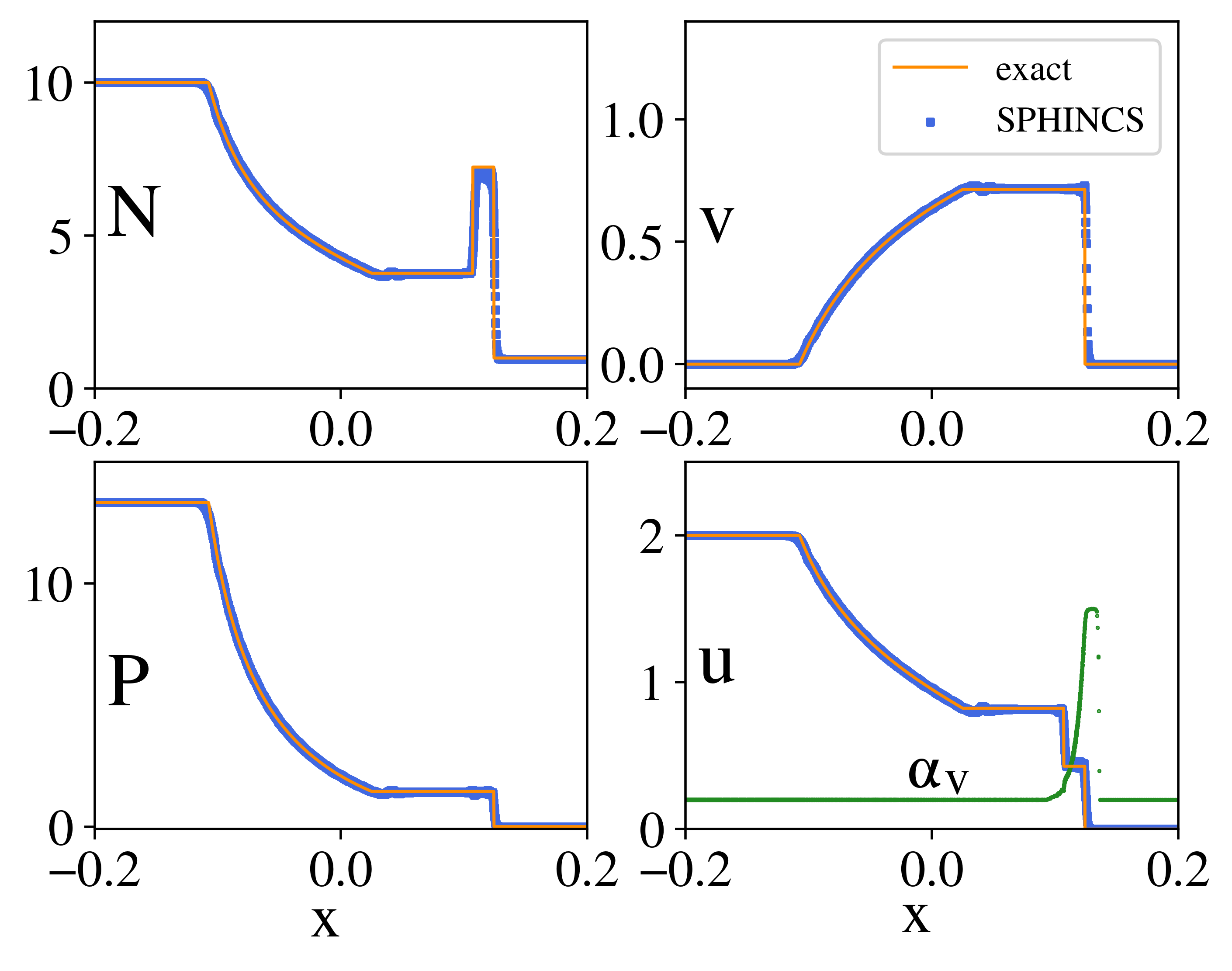
Figure 4: 3D, relativistic shocktube test. The exact solution is shown as orange lines, while the numerical results for the computing frame baryon number density $N$, the velocity $v$, the pressure $P$ and the specific internal energy $u$ are shown as blue squares. All particles are shown. We also show in last panel the dissipation parameter $\alpha$ (in green): it ”switches on” just directly ahead of the shock, and then very quickly decays to the floor level value.

With exactly known solutions, shock tubes are excellent tests to verify a correct implementation of the hydrodynamic equations. We perform here a 3D relativistic version of “Sod’s shocktube” Sod (1978) which has become a widespread benchmark for relativistic hydrodynamics codes Marti and Müller (1996); Chow and Monaghan (1997); Siegler and Riffert (2000); Del Zanna and Bucciantini (2002); Marti and Müller (2003). The test uses a polytropic exponent $\Gamma=5/3$ and as initial conditions

$$\left[N,P\right]=\left\{\begin{array}[]{ll}\left[10,\frac{40}{3}\right],&{\rm for\;}x<0\\ \left[1,10^{-6}\right]&{\rm for\;}x\geq 0,\end{array}\right.$$ (97)

with velocities initially being zero everywhere. We place particles with equal baryon numbers on close-packed lattices as described in Rosswog (2015a), so that on the left side the particle spacing is $\Delta x_{L}=0.0005$ and we have 12 particles in both $y$- and $z$-direction. This test is performed with the full 3+1 dimensional code, but using a fixed Minkowski metric. The result at $t=0.15$ is shown in Fig. 4 with the SPHINCS_BSSN  results marked with blue squares and the exact solution Marti and Müller (2003) with the orange line. In the last panel we also show the dissipation parameter $\alpha_{v}$ (in green): it switches on sharply just ahead of the shock front and then, once the shock wave has passed, very rapidly decays to the chosen floor value. Overall there is very good agreement with practically no spurious oscillations. There is only a small amount of ”noise” directly after the shock front. This is to some extent unavoidable, since here the particles have to re-arrange themselves from their pre-shock close-packed configuration into their preferred post-shock configuration which goes along with some mild sideways motion.

0.3.2 Oscillating neutron stars

In order to test the full code, i.e. the relativistic hydrodynamics, the spacetime evolution and their mutual coupling via the mappings from the grid to the particles and from the particles to the grid, we have performed simulations of single oscillating neutron stars. For this problem oscillation frequencies are known from independent, linear perturbation approaches Font et al. (2002) which serve as a measure of the accuracy of our approach. We solve the Tolman-Oppenheimer-Volkoff (TOV) equations Tolman (1939); Oppenheimer and Volkoff (1939) for a star in equilibrium which is then used to set up initial data for the particles and the spacetime grid. Due to truncation error the star does not remain in exact equilibrium and different eigenmodes of the star are excited at eigenfrequencies that depend on the equation of state and the mass of the star. In Font et al. (2002) the frequencies of the fundamental as well as higher harmonic modes (obtained with a linear perturbation code) were reported for a star with the polytropic equation of state $P=K\rho^{\Gamma}$ with $\Gamma=2.0$ . With the choice of $K=100$ and a central density of $\rho_{c}=1.28\times 10^{-3}=7.91\times 10^{14}$g/cm³ we get a star with a gravitational mass of 1.4 M_⊙ and a baryonic mass of 1.506 M_⊙.
We performed 3 simulations with varying resolution of both the number of particles and the grid. For the particles we used 500k (low), 1M (medium) and 2M (high) particles. In all cases we used a grid with outer boundaries (in all directions) at 160 in code units, corresponding to 236 km. We used 4 levels of refinement with the star being completely contained within the finest grid. The resolution on the finest grid was 0.4$\approx$ 590 m (low), 0.317$\approx$ 468 m (medium) and 0.25$\approx$ 369 m (high). The smallest smoothing length in each case was about 310 m (low), 255 m (medium) and 208 m (high). We evolved the stars up to physical times of almost 30 ms.

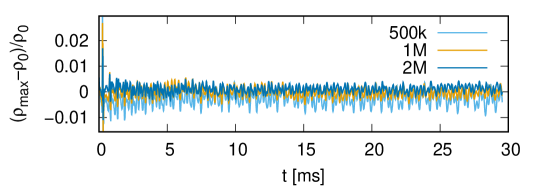
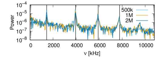
Figure 5: Top plot: The relative difference between the maximal density $\rho_{\mathrm{max}}$ and the initial maximal density, $\rho_{0}$, for the TOV star as function of time in units of ms. Bottom plot: The power in the Fourier spectrum as function of frequency in units of kHz. In both plots the light blue line is for 500k, the orange is for 1M and the dark blue is for 2M particles. In the bottom plot, the vertical lines indicate (from left to right) the position of the expected frequency for the fundamental mode at 1.442 kHz, the first harmonic at 3.955 kHz, the second harmonic at 5.916 kHz and the third harmonic at 7.776 kHz. Note that another peak at around 9.54 kHZ seem to get more sharply defined at higher resolution, so we predict that a fourth harmonic mode exists at this frequency.

The results are shown in Fig. 5. In the top plot we show the relative difference between the maximal density, $\rho_{\mathrm{max}}$, and the initial maximal density, $\rho_{0}$, as a function of time for the three runs. Here light blue is low, orange is medium and dark blue is high resolution. As expected, the amplitudes of the oscillations decrease with higher resolution ($\approx 0.002$ for 2M particles) and multiple modes at different frequencies are excited. Taking a Fourier transform of $(\rho_{\mathrm{max}}-\rho_{0})/\rho_{0}$ results in the spectrum shown in the bottom plot of Fig. 5. We clearly see four distinct peaks at frequencies that agree very well with the frequencies of the fundamental mode and the three first harmonics that were reported in Font et al. (2002) using a linear perturbation code. In addition we see another peak at an even higher frequency. We suspect that this is a fourth harmonic mode with a frequency of about 9.54 kHZ. The reference values for the known frequencies are indicated with black vertical lines in the plot. Quantitative error measures for the known frequencies are provided in Table 0.3.2. Note that even at the lowest resolution, the frequencies agree to better than 1% with the reference solution and they further improve with resolution.

Table 1: Oscillation frequencies: fundamental mode (F), first, second and third harmonic (H1, H2, and H3) frequencies (from Font et al. (2002)) are given in Hz, numbers in brackets refer to the relative deviations from the reference values in percent. Note that even at the lowest resolution the agreement of SPHINCS_BSSN results with the reference solution is better than 1%.

Reference/particle number	F	H1	H2	H3
results Font et al. (2002)	1442	3955	5916	7776
500k	1437   (0.3)	3938   (0.4)	5889   (0.4)	7714   (0.8)
1M	1439   (0.2)	3942   (0.3)	5896   (0.3)	7736   (0.5)
2M	1440   (0.1)	3946   (0.2)	5902   (0.2)	7750   (0.3)

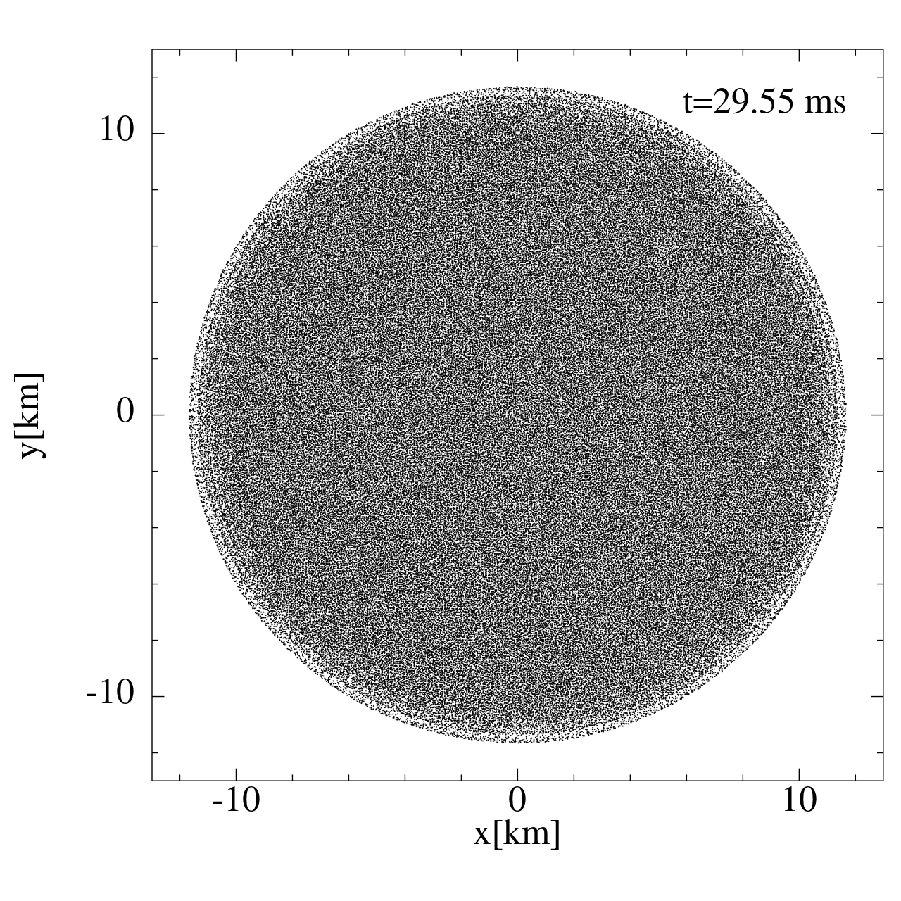
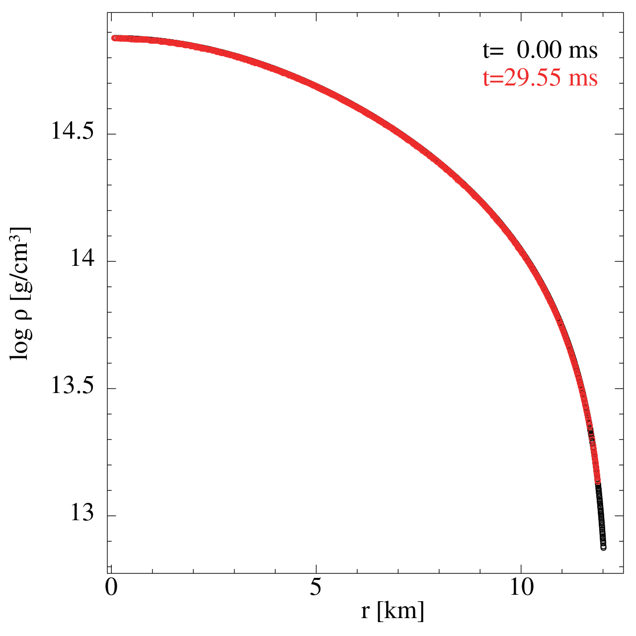
Figure 6: The left plot shows a projection of the particle distribution of a 2M particle simulation (all particles are shown) at the final time, $t=29.55$ ms. This time corresponds to more then 42 oscillation periods of the fundamental mode. Note that the neutron star surface has remained perfectly well behaved and the density distribution at late time (red) is nearly identical to the initial condition (black).

In Fig. 6 we show a projection to the $xy$-plane of the particle distribution at the end of the simulation (left plot) and a comparison between the initial (black) and final (red) density as a function of radius (right plot). The final time, $t=29.55$ ms, corresponds to more than 42 oscillation periods at the fundamental mode frequency. Note that, despite the long evolution time, the surface of the TOV star is extremely well behaved with no ”outlier” particles (the plot shows all the particles). In contrast, the neutron star surface in Eulerian simulations is a perpetual source of numerical trouble where often (completely spurious) ”winds” are driven away from the star. From the right plot it is clear that the density distribution has changed very little over the duration of the simulation. The main difference is that particles near the surface have moved inward by a very small amount compared to the starting position, but overall the density distribution has remained very well-behaved and is essentially identical to the initial condition.

0.3.3 Neutron star mergers

One of the key motivations behind the SPHINCS_BSSN development efforts are the multi-messenger signatures of merging neutron star binaries. We will show here two examples, one merger where the remnant remains stable until the end of the simulation and another one where the encounter results in a prompt collapse to a black hole.

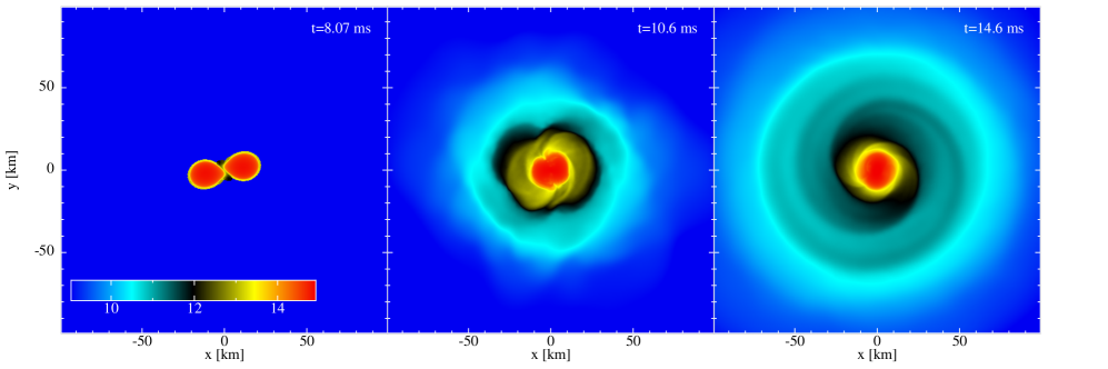
Figure 7: Merger of an irrotational binary system with $2\times 1.3$ M_⊙ with the APR3 equation of state. Shown is the density distribution in the orbital plane.

Merger with stable remnant

As an example of a neutron star merger that results in a surviving remnant, we show a binary of 2$\times$1.3 M_⊙ with the piecewise polytropic representation Read et al. (2009) of the APR3 equation of state Akmal, Pandharipande, and Ravenhall (1998), where we add a thermal pressure/internal energy component with a thermal polytropic exponent $\Gamma_{\rm th}=1.75$, see Fig. 7. The spacetime/matter initial conditions for this binary system were calculated using the FUKA code Papenfort et al. (2021), subsequently the particles were placed according to the ”artificial pressure method” Rosswog (2020a); Rosswog, Torsello, and Diener (2023) with the code SPHINCS$\_$ID. We start from an initial separation $a_{0}$= 45 km and use 2 million SPH particles to model the matter evolution while for the spacetime evolution we initially employ seven levels of mesh refinement with 193 points in each direction. During the merger and the subsequent evolution, the spacetime becomes more extreme and SPHINCS_BSSN automatically increases the number of refinement levels to eight, see Sec. 2.5 in Rosswog, Torsello, and Diener (2023) for more information on our mesh refinement algorithm. Fig. 7 shows the density evolution (in the orbital plane) and in the top of Fig. 0.3.2 we show how the maximum density and the minimum value of the lapse function evolve. As the stars approach each other, the lapse continuously decreases, while the peak density stays essentially constant. The merger results in a strong initial compression (by $\sim$ 25% in the density), a subsequent ”bounce back” during which the peak density drops below the initial single-star density, and then a continuous increase which levels off to a constant value at $\sim$ 15 ms after the merger. The evolution of the lapse function during the merger is anti-correlated with the peak density: during maximum compression the laps drops to a minimum value of 0.42 and reaches after $\sim 15$ ms an asymptotic value of 0.45. In the bottom plot of Fig. 0.3.2 we show, in light blue, the plus- and, in orange, the cross-polarization of the strain times the distance to the source, $r$. The gravitational waves has been extracted from the simulation via the Newman–Penrose Weyl scalar $\Psi_{4}$ at an extraction sphere of $R_{\mathrm{extr}}=150\approx 221.5$ km, see the appendix A of Diener, Rosswog, and Torsello (2022) for more details and we have used kuibit Bozzola (2021) for their analysis. At the earliest stages ($t<-7$ ms; $t=0$ marking the peak GW emission) there is a small spurious transient introduced by the initial conditions, subsequently one recognizes the expected ”chirp” signal with a long ring-down phase.

Figure 8: Top: evolution of the peak density and minimum lapse value during the merger of the 2$\times$1.3 M_⊙ merger with APR3 equation of state. Bottom: corresponding gravitational wave amplitudes (multiplied with the distance to the source).

Merger with prompt black hole formation

As an example of a system that undergoes prompt collapse to a black hole, we show the merger of a 2$\times$1.5 M_⊙ binary with the same equation of state, initial separation, particle number and initial grid setup as in Sec. 0.3.3. As this system is massive enough to undergo prompt collapse to a black hole, more refinement levels are added automatically as the collapse proceeds until, at the end, we have 11 levels of refinement. Again see Sec. 2.5 in Rosswog, Torsello, and Diener (2023) for the details.

Figure 9: Top plot: we show in blue (left axis) the maximal density, $\rho_{\mathrm{max}}$, and in orange (right axis) the lapse, $\alpha$, as function of time for the system with two 1.5 M_⊙ neutron stars with the APR3 equation of state. Bottom plot: we show in blue the plus-polarization, $h_{+}$, and in orange the cross-polarization, $h_{\times}$, of $r$ times the gravitational wave strain.

In the top plot of Fig. 0.3.2 we show the maximal density, $\rho_{\mathrm{max}}$, (light blue, left axis), and the lapse, $\alpha$, (orange, right axis) as function of time. As can be seen the lapse starts collapsing right after the merger while the maximal density starts to increase dramatically. The collapsing remnant requires a rapid decrease in the numerical time step as described in Sec. 2.5 in Rosswog, Torsello, and Diener (2023). Once the lapse value of a particle decreases below $\alpha_{\mathrm{dust}}=0.05$, we convert it to ”dust”, which means that we ignore the particle’s internal energy and pressure contribution. This makes the conservative-to-primitive recovery trivial. Below $\alpha_{\rm cut}=0.02$ we remove particles from the simulations. As can be double-checked by calculating a posteriori the apparent horizon, this procedure is safe and does not lead to notable artifacts. During the collapse we reach a maximal density of $\rho_{\mathrm{max}}=5\times 10^{16}$ g/cm³ before the removal of particles kicks in. At the end of the simulation about $7\times 10^{-4}$ M_⊙ of material are still outside the black hole out of which about $2\times 10^{-4}$ M_⊙ are unbound, and some fraction of which has speeds exceeding $0.7c$. The remaining bound material is expected to fall into the black hole eventually.

In the bottom plot of Fig. 0.3.2 we show, in light blue, the plus- and, in orange, the cross-polarization of $r$ times the strain extracted from the simulation at an extraction sphere of $R_{\mathrm{extr}}=150\approx 221.5$ km. Note that, in both the bottom and the top plot, the data is shifted so that the time of maximal gravitational wave power corresponds to $t=0$. The waveform initially ($-7<t<-5.5$ ms) shows some spurious waves from the initial data, but then shows a clean ”chirping” inspiral, the merger ($-0.5<t<0.6$ ms) and, finally, the black hole ringdown ($t>0.6$ ms).

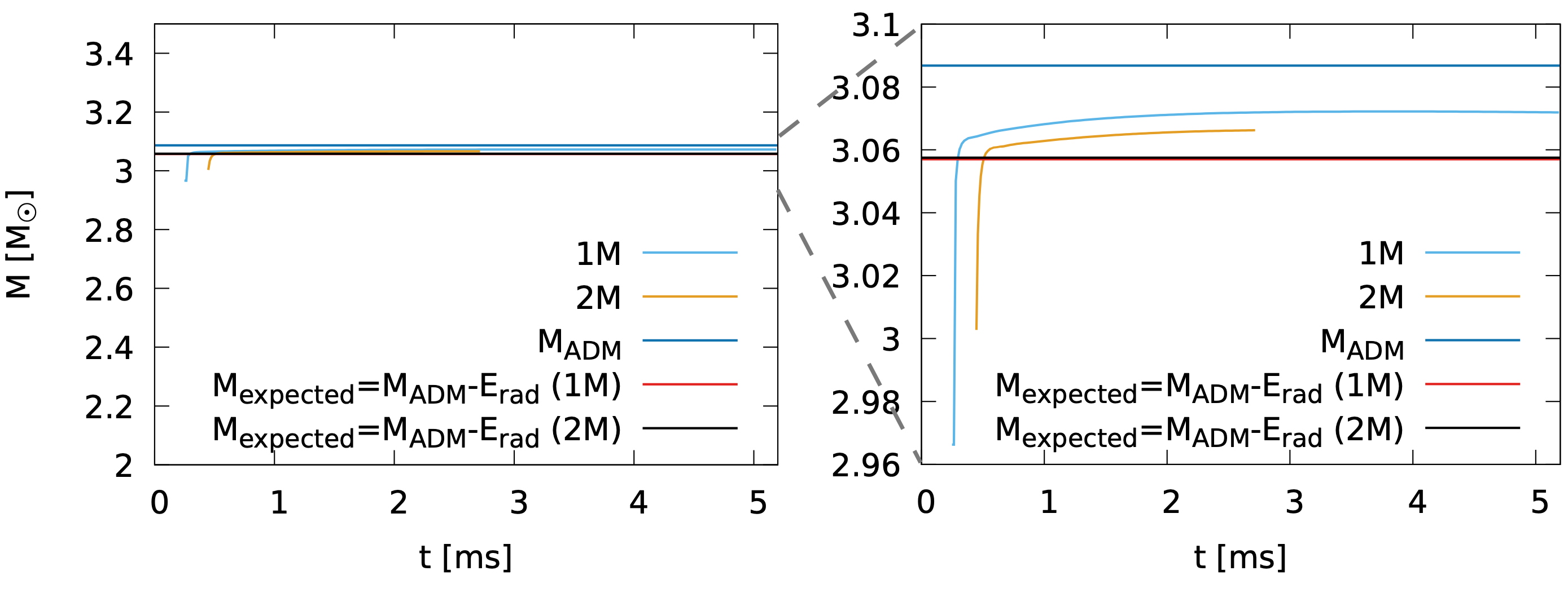
Figure 10: The mass of the black hole (including rotational energy) as function of time (the time has been shifted so zero corresponds to the time of maximal gravitational wave power; left panel is zoom-in of right panel). The orange curve is for the 2M particle runs mentioned earlier, while the light blue curve is for a lower resolution run with 1M particles. The dark blue curve shows the initial ADM mass of the system, while the black and red curves shows the initial ADM mass minus the radiated gravitational wave energy, i.e. the expected final mass of the black hole, as determined by the 2M and 1M runs, respectively.

We have written a reader for spacetime data for the Einstein Toolkit Löffler et al. (2012) to analyze the properties of the black hole that forms. We first used AHFinderDirect Thornburg (1996, 2004) to find the apparent horizon and, once found, QuasiLocalMeasures Dreyer et al. (2003); Schnetter, Krishnan, and Beyer (2006) to calculate the spin and total mass of the black holes. The result is shown in Fig. 10. Here we show the total mass of the black hole for the 2M particle run in orange, the result of a lower resolution 1M particle run is shown in light blue. As can be seen the mass of the black hole grows rapidly at first then slows down and eventually levels off. The dark blue line shows the ADM mass of the initial data, while the black and red lines shows the initial ADM mass minus the energy radiated away in gravitational waves as calculated from the 2M (black) and 1M (red) runs. This is the expected final mass, $M_{\mathrm{final}}$, of the black hole. Both cases produce final black hole masses very close to this value with the 2M run reproducing it to within 0.3 %. For even better agreement, higher resolution would be needed. In the higher resolution run, the final dimensionless spin parameter is $a/M\approx 0.75$.

0.4 Summary and outlook

We have presented here the main methodological elements of the Lagrangian numerical relativity code SPHINCS_BSSN. This code evolves the spacetime in a very similar fashion to standard Eulerian codes, in particular by solving the BSSN equations Alcubierre (2008); Baumgarte and Shapiro (2010) on an adaptive mesh. The major difference to more conventional numerical relativity codes is that the fluid is evolved by means of Lagrangian particles. This has major advantages for tracking and evolving the matter that is ejected in a neutron star merger. This matter, although only a relatively small fraction ($\sim$1%) of the binary mass, is responsible for all the electromagnetic emission and therefore of paramount importance for predicting the multi-messenger signatures on compact binary mergers. This mixed methodology with both particles and adaptive mesh, however, requires an accurate information exchange between the particles and the grid points and this has been one of the major challenges of the development process. As described in Sec. 0.2.3, we have found a way that produces accurate and robust results. To demonstrate the proper functioning of the hydrodynamic part of SPHINCS_BSSN we have performed 3D shock tube tests which show very good agreement with the exact solution and thereby demonstrate the accurate functioning of the hydrodynamic part. Neutron star oscillations where the full spacetime is evolved are a good test for scrutinizing both the spacetime evolution and the coupling of spacetime and hydrodynamics, since measured oscillation frequencies can be compared against accurately known values from independent approaches. We have evolved a neutron star for $\sim 30$ ms and measured its oscillation frequencies. We find excellent agreement with the results of Font et al. (2002): even at low resolution all frequencies agree already to better than 1% and become increasingly more accurate with higher resolution. The neutron star remains essentially perfectly in its initial state and its surface remains very well-behaved without any artifacts. This is a major advantage of SPHINCS_BSSN compared to Eulerian codes. We have further performed two binary neutron star simulations, one where a stable remnant survives and another one where a black hole forms promptly.

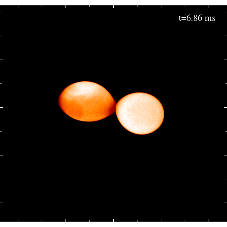
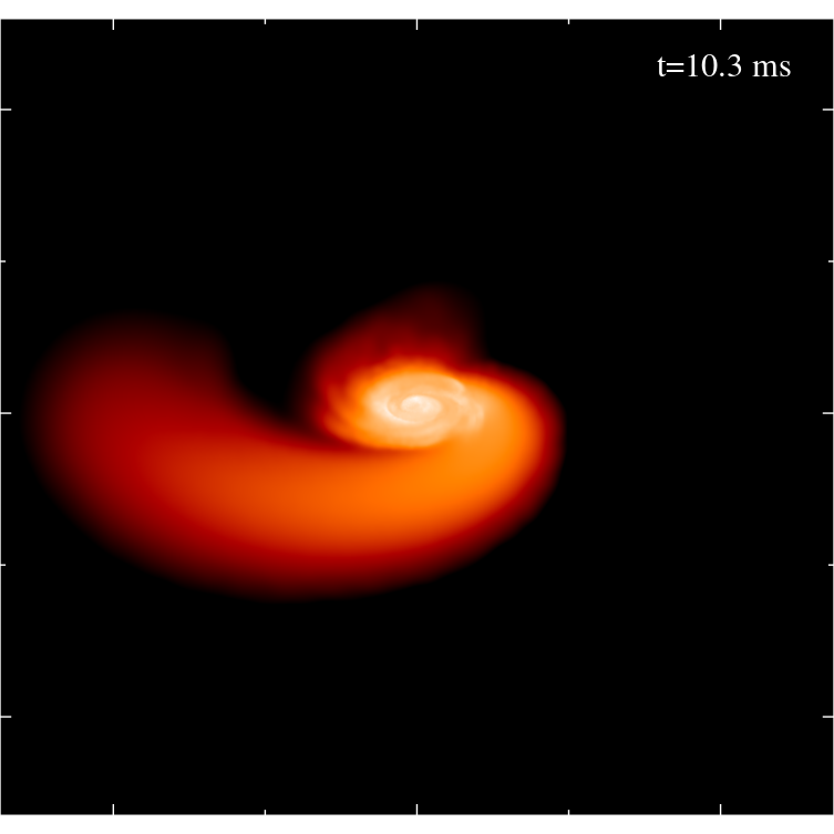
Figure 11: Volume rendering of an equal mass ($2\times 1.3$ M_⊙) binary merger where one of the stars (the left star in the left panel) is rapidly spinning ($\chi_{1}=0.5$) while the other is not ($\chi_{2}=0$). The multi-messenger signatures of such systems are explored in detail in Rosswog et al. (2023).

After an extensive phase of scrutinizing and further improving our methodology, we have recently begun to simulate astrophysical systems Rosswog and Korobkin (2024). Fig. 11 shows a example of a neutron star binary ($2\times 1.3$ M_⊙, APR3 EOS) where one star is rapidly spinning with dimensionless spin parameter $\chi_{1}=0.5$ while the other star has no spin ($\chi_{2}=0$). Such binaries with only one millisecond neutron star are not just a mere academic possibility, but they likely form in dense stellar environments such as globular clusters via binary-single exchange encounters Rosswog et al. (2023). The large majority of neutron stars observed in globular clusters are rapidly spinning and encounters between a binary, consisting of a spun-up neutron star and a low-mass companion, and another neutron star can easily lead to the exchange of the low mass companion with the neutron star. According to our estimates Rosswog et al. (2023), such binaries may account for approximately $\sim 5$% of the merging neutron star systems. Such mergers show a number of distinct signatures in their multi-messenger signals: they dynamically eject approximately an order of magnitude more matter and therefore produce particularly bright kilonovae. Since the collision itself is less violent they produce a smaller amount of fast ejecta ($>0.5c$) and therefore weaker blue/UV kilonova precursors Metzger et al. (2015). The GW-emission is substantially less efficient and therefore one can expect a longer lived central remnant and one may speculate that such mergers may be related to long GRBs that produce kilonova emission such as GRB 211211A Rastinejad et al. (2022) and GRB 230307A Levan et al. (2024). Future development efforts of SPHINCS_BSSN include improvements of its parallelization and the implementation of further physics ingredients such as, for example, more realistic nuclear matter equations of state and neutrino transport.