Decentralized Personalized Federated Learning based on a Conditional ‘Sparse-to-Sparser’ Scheme

Abstract

Decentralized Federated Learning (DFL) has become popular due to its robustness and avoidance of centralized coordination. In this paradigm, clients actively engage in training by exchanging models with their networked neighbors. However, DFL introduces increased costs in terms of training and communication. Existing methods focus on minimizing communication often overlooking training efficiency and data heterogeneity. To address this gap, we propose a novel sparse-to-sparser training scheme: DA-DPFL. DA-DPFL initializes with a subset of model parameters, which progressively reduces during training via dynamic aggregation and leads to substantial energy savings while retaining adequate information during critical learning periods.

Our experiments showcase that DA-DPFL substantially outperforms DFL baselines in test accuracy, while achieving up to $5$ times reduction in energy costs. We provide a theoretical analysis of DA-DPFL’s convergence by solidifying its applicability in decentralized and personalized learning. The code is available at:https://github.com/EricLoong/da-dpfl

I Introduction

Large-scale Deep Neural Networks (DNNs) have gained significant attention due to their high performance on complex tasks. The Vision Transformer, ViT-4 [1] by Google is a prime example of achieving a new state-of-the-art on ImageNet [2] with top-1 accuracy of $90.45\%$. The success of centralized training of DNNs motivated the counterpart decentralized training based on Federated Learning (FL) [3]. FL involves distributed clients’ data in DNN training addressing challenges like privacy [4] by transmitting only model weights and/or gradients instead of raw data. However, FL faces two fundamental challenges [5]: expensive communication and statistical heterogeneity. Reducing the communication cost due to clients disseminating big-sized DNNs can be achieved by compressing information exchange while attaining model convergence. Gradient sparsification and quantization [6, 7] significantly reduce communication cost. Model pruning [8, 9, 10, 11, 12] not only reduces communication cost but also accelerates local training. To alleviate statistical heterogeneity and cope with non-independent and identically distributed (non-i.i.d.) data, Personalized FL (PFL) emerges to allow a local (personalized) model per client rather than a global one shared among clients. Though PFL is still in its infancy, a plethora of works [13, 11, 14, 15, 16, 17, 12] shows its efficiency in data heterogeneity.

FL is classified into Centralized FL (CFL) and Decentralized FL (DFL), differentiated by clients’ communication methods during training. CFL, exemplified by FedAvg [3], involves a central server coordinating client model aggregation, posing risks of server-targeted attacks and a single point of failure. In contrast, DFL [18] offers privacy enhancements and risk mitigation by enabling direct, dynamic, non-hierarchical client interactions within various network topologies such as line/bus, ring, star, or mesh. To address communication cost, model/gradient compression-based DFL has been proposed [11, 19, 20, 21], where local models are pruned/quantized to achieve competitive performance similar to dense (non-pruned) models. These approaches match communication costs for the busiest servers as CFL, having higher overall communication and training costs attributed to decentralized hybrid topology (each client can act as a server). Although DFL with pointing protocol, i.e., learning from previously trained models of clients in a sequential line one-peer-to-one-peer, can expedite convergence [18], it struggles with data heterogeneity. Overall, while FL frameworks target learning from decentralized data, they often overlook either statistical heterogeneity, as in DFL, or efficient training and communication, as in PFL. This highlights the need for an integrated approach that effectively balances communication, training efficiency, and data heterogeneity across different FL paradigms. We contribute with a novel Dynamic Aggregation Decentralized PFL framework, coined as DA-DPFL, that (i) further reduces communication and training costs, (ii) expedites convergence, and (iii) overcomes data heterogeneity. DA-DPFL incorporates two main elements: a fair dynamic scheduling for aggregation of personalized models and a dynamic pruning policy. The innovative scheduling policy allows clients in DA-DPFL to reuse trained models within the same communication round, which significantly accelerates convergence. Moreover, DA-DPFL involves optimized pruning timing to conduct further pruning, i.e., sparse-to-sparser training, which does not violate clients’ computing capacities while achieving communication, training, and inference efficiency. The trade-off is the controlled latency incurred as some clients await the completion of tasks by their neighbors. We comprehensively assess and compare DA-DPFL with baselines in CFL and DFL to showcase the advantage of dynamic pruning and aggregation in PFL.
Our major technical contributions are: (i) We innovatively align a dynamic aggregation framework to allow clients reuse previous models for local training within the same communication round. (ii) By measuring model compressibility, we propose a further pruning strategy, which effectively accommodates and extends existing sparse training techniques in DFL. (iii) Compared with both CFL and DFL baselines, our comprehensive experiments showcase that DA-DPFL achieves comparative or even superior model performance across various tasks and DNN architectures. (iv) The proposed learning method with dynamic aggregation achieves the highest energy and communication efficiency. (v) We provide a theoretical convergence analysis, which aligns with experimental observations.

II Related Work

Efficient FL: In distributed ML, communication and training costs are significant challenges. LAQ [6] and DGC [7] methods reduce communication costs through gradient quantization and deep gradient compression techniques, respectively. Model compression, notably pruning, plays a key role in alleviating device storage constraints, as demonstrated by PruneFL [8], FedDST [22], and FedDIP [10], which achieve sparsity in model pruning. pFedGate [23] addresses the challenges by adaptively learning sparse local models with a trainable gating layer, enhancing model capacity and efficiency. FedPM [9] and FedMask [12] focus on efficient model communication using probability masks; with FedMask providing personalized, sparse DNNs for clients and FedPM employing Bayesian aggregation. However, while significant advancements have been made in reducing communication costs [9, 6, 7, 12], only a few methods [8, 10, 23] address reducing training costs through sparse mask learning.

Personalized FL: In FL, addressing data heterogeneity necessitates personalization of global model as achieved by e.g., FedMask [12], FedSpa [15], and DisPFL [11] using personalized masks. Ditto [14] offers a fair personalization framework through global-regularized multitask FL, while FOMO [13] focuses on first-order optimization for personalized learning. FedABC [16] employs a ‘one-vs-all’ strategy and binary classification loss for class imbalance and unfair competition, while FedSLR [17] integrates low-rank global knowledge for efficient downloading during communication. However, such approaches increase training costs highlighting the need for more efficient training methods.

Decentralized FL: Since the work [24], DFL emerged as a robust distributed learning paradigm, enabling clients to collaboratively train models with their neighbors, thereby enhancing privacy and reducing reliance on central servers. In DFL, increased client interaction leads to methods like DFedAvgM [19], which extends FedAvg to decentralized context with momentum SGD, and BEER [20] for non-convex optimization that enhances convergence through communication compression and gradient tracking. GossipFL [25] uses bandwidth information to create a gossip matrix allowing communication with one peer using sparsified gradients, reducing communication. DFedSAM [26] considers utilizing Sharpness-Aware-Minimization (SAM) optimizer, while DisPFL [11] utilizes RigL-like pruning in decentralized sparse training to lower generalization error and communication costs.

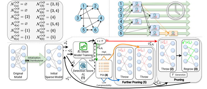
Figure 1: (Top) Client network ($K=6,M=2,N=1$) with reuse indexes $\mathcal{N}_{k(a)}^{(*)t}$ and $\mathcal{N}_{k(b)}^{(*)t}$. Learning schedule: while $N=0$, all nodes train in parallel, i.e., $\mathcal{N}_{k(a)}^{(*)t}=\emptyset$; if $N=1$, node 3 waits for 2, node 5 and 6 for 1; nodes 1, 2, 4 begin parallel training immediately; $N=2$ enables node 6 wait for $1$ and 5, marked with different color. (Bottom) Training process at time $t$ for client $k$. Flow follows $t\in\mathcal{T}$: ‘no’ leads to normal sparse training, ‘yes’ to proposed sparser training. Steps: (1) Detection score calculation using $\omega_{k}^{t}$, determining $t^{*}$; (2) Magnitude-based weight pruning; (3) Gradient-flow-driven weight recovery; (4) PQI evaluation for NN compressibility; (5) Additional pruning based on compressibility level.

III Problem Fundamentals & Preliminaries

Consider a distributed system with $K$ clients indexed by $\mathcal{K}=\{1,2,\ldots,K\}$. The clients are networked given a topology represented by a graph $\mathcal{G}(\mathcal{K},\mathbf{V})$, where the adjacency matrix $\mathbf{V}=[v_{i,j}]\in\mathbb{R}^{K\times K}$ [19] defines the neighborhood $\mathcal{G}_{k}$ of client $k\in\mathcal{K}$, i.e., subset of clients that directly communicate with client $k$, $\mathcal{G}_{k}=\{i\in\mathcal{K}:v_{i,k}>0\}$. An entry $v_{i,k}=0$ indicates no communication from client $i$ to client $k$, i.e., $i\notin\mathcal{N}_{k}$. Note that $v_{i,k}=v_{k,i}$ may not always be valid for $i\neq k$. The topology can be static or dynamic. In our case, we adopt dynamic communication among clients, i.e., entries in $\mathbf{V}^{t}$ depend on (discrete) time instance $t\in\mathbb{T}=\{1,2,\ldots\}$. We define a time-varying and non-symmetric network topology via $\mathbf{V}^{t}=[v_{i,j}^{t}]\in\mathbb{R}^{K\times K}$ accommodating temporal neighborhood $\mathcal{G}_{k}^{t}$ for $k$-th client. We consider a scalable DFL setting with $K$ clients (e.g., mobile devices, IoT devices) with a time-varying topology. Each client $k\in\mathcal{K}$ possesses local data $\mathcal{D}_{k}=\{(\mathbf{x},y)\}$ of input-output pairs $\mathbf{x}\in\mathcal{X}$ and $y\in\mathcal{Y}$, and communicates with neighbours $\mathcal{G}_{k}^{t}$ exchanging models. The problem formulation of PFL (adopting the formulation in [11]) seeks to find the models $\mathbf{\omega}_{k},\forall k\in\mathcal{K}$, that minimize:

$$\min_{\{\mathbf{\omega}_{k}\},k\in[1,K]}f(\{\mathbf{\omega}_{1}\}_{k=1}^{K})=\frac{1}{K}\sum_{k=1}^{K}F_{k}(\mathbf{\omega}_{k}),$$ (1)

where $F_{k}(\mathbf{\omega}_{k})=\mathbb{E}[\mathcal{L}(\mathbf{\omega}_{k};(\mathbf{x},y))|(\mathbf{x},y)\in\mathcal{D}_{k}]$ with expected loss function $\mathcal{L}(.;.)$ between actual and predicted output given local data $\mathcal{D}_{k}$. We depart from ((1)) by adopting model pruning in DFL aiming at eliminating non-essential model weights. This is achieved by utilizing a binary mask $\mathbf{m}$ over a model. Hence, the pruning-based (masked) PFL problem is succinctly formulated as finding the global model $\mathbf{\omega}$ and individual masks $\mathbf{m}_{k},\forall k\in\mathcal{K}$:

$$\min_{\mathbf{\omega},\{\mathbf{m}_{k}\},k\in[1,K]}f(\{\mathbf{\omega}_{k}\}_{k=1}^{K})=\frac{1}{K}\sum_{k=1}^{K}F_{k}(\omega\odot\mathbf{m}_{k}),$$ (2)

where $F_{k}(\omega\odot\mathbf{m}_{k})=\mathbb{E}[\mathcal{L}(\omega\odot\mathbf{m}_{k};(\mathbf{x},y))|(\mathbf{x},y)\in\mathcal{D}_{k}]$; $\odot$ represents the Hadamard product (element-wise product) of two matrices. The individual mask $\mathbf{m}_{k}$ denotes a pruning operator specific to client $k$. Given mask $\mathbf{m}_{k}$, the sparsity $s_{k}\in[0,1]$ of $\mathbf{m}_{k}$ indicates the proportion of non-zero model weights among all weights. The goal of (2) is to seek a global model $\boldsymbol{\omega}$ and individual masks $\mathbf{m}_{k}$ such that the optimized personalized model for each client $k\in\mathcal{K}$ is given by $\boldsymbol{\omega}_{k}=\boldsymbol{\omega}\odot\mathbf{m}_{k}$, while clients communicate at time $t$ only with their neighbors $\mathcal{G}_{k}^{t}$ given the time-varying $\mathbf{V}^{t}$.

IV The DA-DPFL framework

IV-A Overview

We introduce the DA-DPFL framework to tackle the problem in Eq. (2). DA-DPFL not only addresses data heterogeneity efficiently via masked-based PFL but also significantly improves convergence speed by incorporating a fair dynamic communication protocol. Sequential pointing line communication adopts an one-peer-to-neighbors mechanism striking the balance between computational parallelism and delay. As described in [18], two sequential pointing DFL strategies, continual and aggregate, facilitate knowledge dissemination in distributed learning. However, certain challenges are evident as discussed in [18] such as data heterogeneity and non-scalability. Furthermore, the decision on when to apply pruning during training is crucial [27, 28]. While early pruning reduces computational cost, it may adversely affect performance. Choosing an optimal pruning time can enhance both training and communication efficiency, often with minimal performance degradation or even improvements. As elaborated in [11] and [29], a sparser model tends to have a reduced generalization bound characterized by smaller discrepancy between training and test errors. Finding sparser models with lower generalization error, DA-DPFL introduces an innovative dynamic pruning strategy. DA-DPFL addresses data heterogeneity while decreasing the number of communication rounds needed for convergence and achieving high model performance. This comes at a small and controllable delay in learning from the trained models. The processes of DA-DPFL are depicted in Fig. 1 and Algorithm 1.

Remark 1.

The relationship between model sparsity and performance links to the complexity of the task and model architecture. Pruning becomes a necessary solution when there is model redundancy for the given task, aligned with the findings in [11] and [29]. If the model is non-redundant, an increased sparsity invariably affects model performance.

Algorithm 1 The DA-DPFL Algorithm

1:  Input: $K$ clients; $T,E_{l}$ rounds; PQI hyper-param. $\{p,q,\gamma,\eta_{c}\}$, pruning thr $\delta_{pr}$; voting threshold $\delta_{v}$; factors $b,c$; target sparsity $s^{*}$;

2:  Output: Personalized aggregated models $\{\boldsymbol{\tilde{\boldsymbol{\omega}}}_{k}^{T}\}_{k=1}^{K}$.

3:  Initialization: Initialize $\{\mathbf{m}_{k}^{0}\}_{k=1}^{K}$, $\{\boldsymbol{\omega}_{k}^{0}\}_{k=1}^{K}$, $\mathcal{T}\leftarrow\emptyset$

4:  for round $t=1$ to $T$ do

5:     for each client $k$ do

6:        Generate a random reuse index set $\{\mathcal{N}^{t}_{k}\}_{k=1}^{K}$.

7:        Generate a random bijection $\pi^{t}_{k}$ between $\mathcal{N}^{t}_{k}$ and $\mathcal{G}^{t}_{k}$

8:        Form prior and posterior set $\{\mathcal{N}^{(*)t}_{k(a)},\mathcal{N}^{(*)t}_{k(b)}\}$

9:        Form $\{\mathcal{G}^{(*)t}_{k(a)},\mathcal{G}^{(*)t}_{k(b)}\}$ by $\{\mathcal{N}^{(*)t}_{k(a)},\mathcal{N}^{(*)t}_{k(b)},\pi^{-1(t)}_{k}\}$

10:        if $\mathcal{G}_{(a)k}^{(*)t}!=\emptyset$ then

11:           do Wait models from neighbors $\mathcal{G}_{(a)k}^{(*)t}$

12:        end if

13:        Receive neighbor’s models $\boldsymbol{\omega}_{j}^{t},j\in\mathcal{G}_{k}^{t}$

14:        Obtain mask-based aggregated model $\boldsymbol{\tilde{\omega}}_{k}^{t}$.

15:        Compute $\boldsymbol{\tilde{\omega}}_{k,\tau}^{t}$ for $E_{l}$ local rounds.

16:        Calculate $\Delta_{0}^{t}(k)$ and $v_{t}(k)$ based on $\delta_{pr}$.

17:        Broadcast $v_{t}(k)$ to all clients; derive $t^{*}$.

18:        if $t\in\mathcal{T}$ and $s_{k}<s^{*}$ then

19:           Call Algorithm 2 to obtain $\boldsymbol{\tilde{\omega}}_{k,E_{l}}^{t\prime},\mathbf{m}_{k}^{t\prime}$

20:           Update sparsity $s_{k}$

21:        else

22:           Set $(\boldsymbol{\tilde{\omega}}_{k,E_{l}}^{t\prime},\mathbf{m}_{k}^{t\prime})\leftarrow(\boldsymbol{\tilde{\omega}}_{k,E_{l}}^{t},\mathbf{m}_{k}^{t})$

23:        end if

24:        Call Algorithm 3 to update $\mathbf{m}_{k}^{t+1}$

25:        Set $\boldsymbol{\omega}_{k}^{t+1}=\boldsymbol{\tilde{\omega}}_{k,E_{l}}^{t\prime}$

26:     end for

27:     if $t==t^{*}$ then Update $\mathcal{T}$.

28:  end for

IV-B Learning Scheduling Policy

In this section, we outline the scheduling policy adopted for client participation within our framework. This applies to any topological connection, such as a ring or fully-connected network, where neighborhood sets, denoted as $\mathcal{G}_{k}^{t},k\in\{1,2,\ldots,K\}$, are established. It is important to note that DA-DPFL is particularly suited for a time-varying connected topology while remains flexible to accommodate a static topology, represented as $\mathcal{G}_{k}$. At the start of each communication round, denoted by $t$, reuse indexes for neighborhood sets, $\mathcal{N}_{k}^{t}$, are randomly assigned to $M$ clients, where $\lvert\mathcal{G}_{k}^{t}\rvert=\lvert\mathcal{N}_{k}^{t}\rvert=M<K$ and $\mathcal{G}_{k}^{t}\stackrel{{\scriptstyle\pi_{k}^{t}}}{{\leftrightarrow}}\mathcal{N}_{k}^{t}$, where $\pi_{k}^{t}$ is a random bijection mapping. Given $\mathcal{G}_{k}^{t}$ and $\mathcal{N}_{k}^{t}$ are both discrete sets,

$$i=\pi_{k}^{t}(j),$$ (3)

with index $i\in\mathcal{N}_{k}^{t}$ and $j\in\mathcal{G}_{k}^{t}$. It is crucial to acknowledge that $\mathcal{N}_{k}^{t}$ may be equal with $\mathcal{G}_{k}^{t}$ if sets are randomly generated. For simplicity, we let $\mathcal{N}_{k}^{t}=\mathcal{G}_{k}^{t}$ in Fig. 1, where client $k$ is indexed with reuse index $k$. The introduction of $\mathcal{N}_{k}^{t}$ serves to emphasize the independence in the generation of reuse indexes, which are pivotal in guiding the dynamic aggregation process. Note: the criteria for establishing $\mathcal{G}_{k}^{t}$ are influenced by factors e.g., network bandwidth, geographical location, link availability; however, $\mathcal{N}_{k}^{t}$ is independent of these factors. We reassign client indices for each training round.

Within DA-DPFL, a client $k$ may defer the reception of models from some neighbors, contingent upon $\mathcal{N}_{k}^{t}$. We denote $\mathcal{N}_{k}^{t}$ for each client $k$ into two subsets based on the reuse indices of neighboring clients: (a) a prior client subset $\mathcal{N}_{(a)k}^{t}=\{n_{k}^{t}\leq k:n_{k}^{t}\in\mathcal{N}_{k}^{t}\}$, and (b) a posterior client subset $\mathcal{N}_{(b)k}^{t}=\{n_{k}^{t}>k:n_{k}^{t}\in\mathcal{N}_{k}^{t}\}$ (refer to Fig. 1 Top). Should $\mathcal{N}_{(b)k}^{t}=\emptyset$, implying $\mathcal{N}_{(a)k}^{t}=\mathcal{N}_{k}^{t}$, client $k$ awaits the slowest client within $\mathcal{N}_{k}^{t}$ before commencing model aggregation and local dataset training $\mathcal{D}_{k}$. To enhance scalability, we introduce a threshold to allow waiting for, at most, $N$ fastest clients in $\mathcal{N}_{(a)k}^{t}$, where $\lvert\mathcal{N}_{(a)k}^{(*)t}\rvert=N\leq M$. Then, $\mathcal{N}_{(a)k}^{(*)t}\cup\mathcal{N}_{(b)k}^{(*)t}=\mathcal{N}_{k}^{t}$. Conversely, absence of a prior client set ($\mathcal{N}_{(a)k}^{(*)t}=\emptyset$) enables client $k$ to incorporate models from $\mathcal{N}_{(b)k}^{(*)t}$ without delay, as illustrated by nodes 1, 2, and 4 in Fig. 1. Based on the bijection mapping between $\mathcal{N}_{k}^{t}$ and $\mathcal{G}_{k}^{t}$, $\mathcal{G}_{(a)k}^{(*)t}$ is obtained. Therefore, DA-DPFL achieves a hybrid scheme between continual learning with delayed aggregation and immediate aggregation, i.e., dynamic aggregation. Continual learning is achieved by gradual learning of the models from clients in client $k$’s prior set. The benefit obtained is the sequential knowledge transfer from clients in the prior set. This comes at the expense of a potential delay to client $k$ for aggregating the models from $\mathcal{G}^{(*)t}_{k(a)}$. On the other hand, the models of the clients from the posterior set are independently sent to client $k$, without any delay achieving training parallelism.

Remark 2.

DA-DPFL learning schedule diverges from traditional FL paradigms. In our example, at time $t$, nodes $\{1,2,4\}$ engage in simultaneous (parallel) training, while nodes $\{3,5,6\}$ await model reuse from preceding clients. This methodology allows subsequent nodes to train concurrently with preceding ones, as shown by nodes $\{5,6\}$ training in tandem with node $3$. The introduction of a cutoff value $N$ endows our waiting policy with controllability. If $N=0$, DA-DPFL operates as a parallel FL system with sparse training; while $N=M=K$ transits DA-DPFL to a sequential FL.

IV-C Time-optimized Dynamic Pruning Policy

Alongside scheduling of local training and gradual model aggregation achieved by prior and posterior neighbors per client, we introduce a dynamic pruning policy. The initial mask $\mathbf{m}_{k}^{0},\forall k$, is set up in accordance with the Erdos-Renyi Kernel (ERK) distribution [30]. Subsequently, masks are removed and re-grown based on the importance scores, which are computed from the magnitude of model weights and gradients. This strategy is an extension of the centralized RigL [30] to DA-DPFL as elaborated in Appendix -B (line:24) in Algorithm 1. We devise a method that is orthogonal to other fixed-sparsity training methods like RigL facilitating further pruning. The Sparsity-informed Adaptive Pruning (SAP) in [31] introduces the PQ Index (PQI) to assess the potential ‘compressibility’ of a DNN (line:19; Appendix -A). DA-DPFL leverages PQI by integrating within DFL, which addresses the heterogeneity of various local models by adaptively pruning different models. In centralized learning, EarlyCrop’s analysis [28] on pruning scheduling relies on sufficient information during critical learning periods, while CriticalFL [32] advocates for an early doubling of information transmission. EarlyCrop leverages between gradient flow and neural tangent kernel to facilitate seamless transition into model pruning. We adjust the pruning time detection score as:

$$\frac{\lvert\Delta_{0}^{t}-\Delta_{0}^{t-1}\rvert}{\lvert\Delta_{0}^{1}\rvert}<\delta_{pr};\Delta_{0}^{t}:=\|\boldsymbol{\omega}^{t}-\boldsymbol{\omega}^{0}\|^{2},$$ (4)

where $\delta_{pr}$ is a predefined threshold. In DA-DPFL with $K$ clients, we introduce a voting majority rule, where the client $k$’s vote is defined as:

$$v_{t}(k)=\begin{cases}1&\text{if }\frac{\lvert\Delta_{0}^{t}(k)-\Delta_{0}^{t-1}(k)\rvert}{\lvert\Delta_{0}^{1}(k)\rvert}<\delta_{pr},\\ 0&\text{otherwise.}\end{cases}$$ (5)

Hence, the first time to prune is determined by $K$ clients as: $t^{*}=\min\{t:\frac{1}{K}\sum_{k=1}^{K}v_{t}(k)<\delta_{v}\}$ where $\delta_{v}$ represents the ratio threshold for voting. Given the first pruning time $t^{*}$, DA-DPFL determines the frequency of pruning for rounds $t>t^{*}$. Based on the influence of early training phase, a.k.a. critical learning period [33] on the local curvature of the loss function in DNNs, our strategy permits a low pruning frequency during the initial stages which intensifies pruning as model approaches convergence. This balance between communication overhead and model performance yields an optimal pruning frequency that varies across tasks and model architectures. We define the pruning frequency, i.e., the gap between consecutive pruning events, and in turn the pruning times by non-evenly dividing the rest of the horizon $T-t^{*}$:

$$I_{\tau}:=\lceil\frac{t^{*}+b}{c^{\tau-1}}\rceil,\tau\in\{\mathbb{Z}_{\geq 1}\}.$$ (6)

Parameter $b>0$ delays the optimal first pruning time, $c>0$ is a scaling factor to adjust pruning frequency. The $p$-th pruning time $t_{p}$ with $t_{p}>t^{*}$, is $t_{p}=\sum_{\tau=1}^{p}I_{\tau}$ obtaining the pruning times set $\mathcal{T}=\{t_{1},\ldots,t_{p}:t^{*}<t_{p}<T\}$.

IV-D Masked-based Model Aggregation

For notation compatibility, following the model aggregation operator in DisPFL[11] and FedDST [22], the client $k$’s aggregated model $\boldsymbol{\tilde{\omega}}_{k}^{t}$ derived from the models of client $k$’s neighbors in $\mathcal{G}^{t}_{k}$ at round $t$ based on masked local model is:

$$\boldsymbol{\tilde{\omega}}_{k}^{t}=\Big{(}\frac{\sum_{j\in\mathcal{G}_{k+}^{t}\boldsymbol{\omega}_{j}^{t}}}{\sum_{j\in\mathcal{G}_{k+}^{t}\mathbf{m}_{j}^{t}}}\Big{)}\odot\mathbf{m}_{k}^{t},$$ (7)

where $\mathcal{G}_{k+}^{t}=\mathcal{G}_{k}^{t}\cup\{k\}$ is client $k$’s neighborhood including client $k$. The local training rounds $\tau\in E_{l}$ based on the obtained $\boldsymbol{\tilde{\omega}}_{k}^{t}$ is: $\boldsymbol{\tilde{\omega}}_{k,\tau+1}^{t}=\boldsymbol{\tilde{\omega}}_{k,\tau}^{t}-\eta(\mathbf{g}_{k,\tau}^{t}\odot\mathbf{\mathbf{m}_{k}^{t}})$, where $\mathbf{g}_{k,\tau}^{t}$ is the gradient of local loss function $F_{k}(\cdot)$ w.r.t. $\boldsymbol{\tilde{\omega}}_{k,\tau}^{t}$.

V Theoretical Analysis

Assumption 1.

$\mu$-Lipschitz-continuity: $\forall\boldsymbol{\omega}_{1},\boldsymbol{\omega}_{2}\in\mathbb{R}^{d}$, $\forall k\in\lvert K\rvert,\mu\in\mathbb{R}:\|\nabla f_{k}(\boldsymbol{\omega}_{1})-\nabla f_{k}(\boldsymbol{\omega}_{2})\|\leq\mu\|\boldsymbol{\omega}_{1}-\boldsymbol{\omega}_{2}\|$.

Assumption 2.

Bounded variance for gradients: [19] $\forall k\in\lvert K\rvert$ and $\boldsymbol{\omega}\in\mathbb{R}^{d}$:

$$\mathbb{E}[\|\nabla\hat{f}_{k}(\boldsymbol{\omega})-\nabla f_{k}(\boldsymbol{\omega})\|^{2}]\leq\sigma^{2}_{l},$$ (8)

$$\frac{1}{K}\sum_{k=1}^{K}\|\nabla f_{k}(\boldsymbol{\omega})-\nabla f(\boldsymbol{\omega})\|^{2}\leq\sigma^{2}_{g},$$ (9)

$$\frac{1}{K}\sum_{k=1}^{K}\|\nabla\tilde{f}_{k}(\boldsymbol{\omega})-\nabla f(\boldsymbol{\omega})\|^{2}\leq\sigma^{2}_{p},$$ (10)

$\hat{f}(\cdot)$ is the estimated gradients from training data; $\tilde{f}(\cdot)$ is personalized global gradients.

Assumption 3.

The aggregated model $\tilde{\boldsymbol{\omega}}_{k}^{t}$ for client $k$ at iteration $t$ is given by:

$$\tilde{\boldsymbol{\omega}}_{k}^{t} =\left(\frac{\sum_{j\in\mathcal{G}_{k}^{t}}\boldsymbol{\omega}_{j}^{t}}{\sum_{j\in\mathcal{G}_{k}^{t}}\mathbf{m}_{j}^{t}}\right)\odot\mathbf{m}_{k}^{t}=\left(\frac{\sum_{j\in\mathcal{G}_{k}^{t}}\boldsymbol{\omega}_{j}^{t}}{M}\right)\odot\mathbf{m}_{k}^{t}$$ (11)

where $\mathcal{G}_{k}^{t}$ is neighborhood of client $k$ with size $|\mathcal{G}_{k}^{t}|=M$; all local models are sparse, i.e., $\boldsymbol{\omega}_{j}^{t}=\boldsymbol{\omega}_{j}^{t}\odot\mathbf{m}_{j}^{t}$.

Proposition 1.

Assume $\mathcal{K}=\{1,2,\ldots,K\}$ clients, then, exactly $m$ neighbors in $\mathcal{N}_{k}^{t}$ have reuse index less than $k$ follows a hypergeometric distribution with

$$\mathbb{P}(m,k)=\mathbb{P}(|\mathcal{N}_{(a)k}|=m)=\frac{\binom{k-1}{m}\binom{K-k}{M-m}}{\binom{K-1}{M}},$$ (12)

where $m<M$ and $|\mathcal{N}_{(a)k}|$ is subset of $\mathcal{N}_{k}^{t}$ with index less than $k$.

Proof.

See Appendix -C ∎

$\tilde{\boldsymbol{\omega}}_{k}^{t}$ denotes the local personalized aggregated model for the $k$-th client at time $t$; The global aggregated model at time $t$, $\tilde{\boldsymbol{\omega}}^{t}$, is defined as the average of the local aggregated models, i.e., $\tilde{\boldsymbol{\omega}}^{t}=\frac{1}{K}\sum_{k=1}^{K}\tilde{\boldsymbol{\omega}}_{k}^{t}$, where $K$ is the total number of clients. Let $M$ represent the number of clients in the neighborhood. All models are under the setup of DA-DPFL, where (1) the models are sparse; and (2) a new scheduling strategy is adopted. Then, we obtain the following theorem.

Theorem 3.

Under Assumptions 1 to 3, when $T$ is sufficiently large and the stepsize $\eta$ for SGD for training client models satisfies $\eta\leq\sqrt{\frac{1}{12\mu^{2}(M-1)(2M-1)}}$ for $M>1$,

$$\min{\mathbb{E}\|\nabla f(\tilde{\boldsymbol{\omega}}^{t})\|^{2}}$$

$$\leq\frac{2}{T\left(\eta-6S_{1}(\mu-\eta)\right)}\left(\mathbb{E}[f(\tilde{\boldsymbol{\omega}}^{0})]-\min{f}\right)+S_{3},$$ (13)

where $S_{1}=2\eta^{2}M(M-1)\left(\exp{\left(\frac{(3M+2)E_{l}}{4(M^{2}-1)}\right)}-1\right)$, $S_{2}=\frac{1}{2M-1}\sigma^{2}_{l}+3(\sigma^{2}_{g}+2\sigma^{2}_{p})$ , and $S_{3}=\frac{2}{\eta-6S_{1}(\mu-\eta)}\cdot\left[(\mu-\eta)S_{1}S_{2}+\frac{3\mu^{2}\eta^{3}(3M+2)E_{l}}{2(M+1)M}(\sigma_{l}^{2}+\sigma_{g}^{2})\right]$. $f(\tilde{\boldsymbol{\omega}}^{0})$ represents initial global model loss, $\min{f}$ is minimum of loss, $M$ is neighborhood size.

Proof.

See Appendix -E ∎

Remark 4.

Theorem 3 reveals that with sufficiently large $T$, the error due to initial model loss and bounded variance for gradients become negligible. Specifically, if one can choose $\eta=\mathcal{O}(\frac{1}{\mu\sqrt{T}})$, the convergence boundary will be dominated by the rate of $\mathcal{O}\left(\frac{1}{\sqrt{T}}+\frac{\sigma^{2}_{l}+\sigma^{2}_{g}+\sigma^{2}_{p}}{\sqrt{T}}+\frac{\sigma^{2}_{l}+\sigma^{2}_{g}}{T}\right)$.

Remark 5.

Theorem 3 is consistent with two key empirical observations: (i) The number of communication rounds required to attain a specified error level $\varepsilon$ is lower compared to the DisPFL model. Note: This efficiency gain is attributed to the term $S_{1}>\left(e^{\frac{E_{l}}{(2M-2)}}-1\right)$, i.e., no scheduling involved, which emerges from our scheduling strategy. The division of the left-hand side (first and third item) of the inequality by $S_{1}$ results in a reduced error boundary. (ii) Changed ratio is $\frac{3M+2}{2M+2}$. When $M=2$, the ratio simplifies to $\frac{4}{3}$. As $M$ increases, this ratio approaches $\frac{3}{2}$. This indicates that while increasing $M$ enhances the error-bound reduction, the improvement rate diminishes, suggesting a limit to the benefits offered DA-DPFL scheduling.

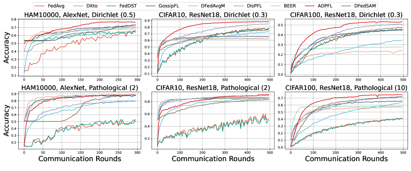
Figure 2: Test (top-1) accuracy of all baselines, including CFLs and DFLs, across various model architectures and datasets.

VI Experiments

VI-A Experimental Setup

VI-A1 Datasets & Models

Our experiments were conducted on three widely-used datasets: HAM10000 [34], CIFAR10, and CIFAR100 [35]. We employed two distinct partition methods, Pathological and Dirichlet, to generate non-i.i.d. scenarios paralleling the approach in [11]. We use Dir for Dirichlet and Pat for Pathological in the following notations. The Dir. partition constructs non-i.i.d. data using a Dir($\alpha$) distribution, with $\alpha=0.3$ for CIFAR10 and CIFAR100, and $\alpha=0.5$ for HAM10000. For Pat. partitioning, several classes $n_{cls}$ are assigned per client: $2$ for CIFAR10 and HAM10000, and $10$ for CIFAR100. To validate the versatility of our pruning methods across various model architectures, we selected AlexNet [36] for HAM10000, ResNet18 [37] for CIFAR10, and VGG11 [38] for CIFAR100, ensuring a comprehensive evaluation across diverse model structures.

VI-A2 Baselines

We compare the proposed methods with baselines including CFL: FedAvg[3], Ditto[14] and FedDST [22], and DFL: GossipFL[25], DFedAvgM[19], DisPFL[11], BEER[20] and DFedSAM[26].

VI-A3 System Configuration

We consider a network of $K=100$ clients and select $M=N=10$ clients (neighbors) per communication round. CFL focuses on the communication between central server and selected clients. DFL mirrors this communication allocating identical bandwidth to each of the busiest clients. This ensures that $10$ clients are active per round matching server’s connection load. All the baseline results are average values for three random seeds of best test model performance. In contrast to CFL, all DFL baselines except DFedSAM are configured with half the communication cost. Our method, FedDST, and DisPFL implement sparse model training for efficiency, which all start with initial sparsity $s_{k}^{0}=0.5$ with $k\in[K]$ for all clients. To ensure a balanced and fair comparison, all DFL benchmarks incorporate personalization by monitoring model performance following local training under randomly time-varying connection in [11].

VI-A4 Hyperparameters

To ensure a fair comparison, we align our experimental hyperparameters with the setups described in [11] and [26]. Unless otherwise specified, we fix the number of local epochs at $5$ for all approaches and employ a Stochastic Gradient Descent (SGD) optimizer with a weight decay set to $5\times 10^{-4}$. The learning rate is initialized at $0.1$, undergoing an exponential decay with a factor of $0.998$ after each global communication round. The batch size is consistently set to $128$ across all experiments. The global communication rounds are conducted 500 times for the CIFAR10 and CIFAR100 datasets, and 300 times for the HAM10000 dataset. We let $\delta_{v}=0.5,b=0,c=1.3$, $\{p,q,\gamma,\eta_{c}\}=\{0.5,1,0.9,1\}$ as suggested by [31], and $\delta_{pr}\in\{0.01,0.02,0.03\}$ for all experiments. In the CFL baseline implementation, the local training for Ditto is bifurcated into two distinct phases: a global model training phase spanning 3 epochs and a personalized model training phase consisting of 2 epochs. Additionally, the update mask reconfiguration interval in FedDST is determined through a grid search within the set $[1,5,10,20]$. In our DFL setup, when algorithms incorporate compression techniques, we manage to reduce half of the busiest communication load. In contrast, GossipFL utilizes a Random Match approach, which entails randomly clustering clients into specific groups. For the optimization algorithm, Momentum SGD is adopted in DFedAvgM and DFedSAM, with a momentum factor $\beta=0.9$. Additionally, a $\rho$ value for DFedSAM is decided by grid search from $[0.01,0.02,0.05,0.1,0.2,0.5]$, following the work for SAM optimizer.

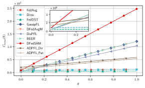
Figure 3: Total cost (energy and time cost, in USD) of DA-DPFL and all baselines evaluated on CIFAR10 against $\theta$.

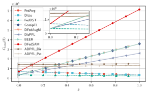
Figure 4: Total cost (energy and time cost, in USD) of DA-DPFL and all baselines evaluated on CIFAR100 against $\theta$.

VI-A5 Cost Simulation

For cost analysis, we utilized an NVIDIA 4090 GPU with 80 TFLOPS and 450 W TDP as a standard to assess clients’ computational power and energy consumption. The architecture anticipates 1 Gbps bandwidth, with client network cards utilizing 1 W, cited from [39]. We derived $C_{\text{time}}$ from Table II and converted $C_{\text{energy}}$ and $C_{\text{time}}$ to monetary units using $(1-\theta)\$/s$ and $\theta\$/J$, illustrated in Fig. 3. To address the gap between theoretical and actual GPU execution times, we performed real-world algorithm executions on the GPU. These revealed a fivefold increase over theoretical times, leading to a correction factor of 5 for computation time, calculated as $T_{\text{comp}}=5\times\frac{D_{\text{FLOP}}}{V_{\text{FLOPS}}}$, and energy, $C_{\text{comp}}=T_{\text{comp}}\times P_{\text{comp}}$. Similarly, in estimating the communication time $T_{\text{comm}}$, we apply the formula $T_{\text{comm}}=\frac{D_{\text{comm}}}{B}$, where $D_{\text{comm}}$ denotes the data volume to be transferred and $B$ signifies the system’s overall bandwidth. Accordingly, the communication energy cost $C_{\text{comm}}$ is determined by $C_{\text{comm}}=T_{\text{comm}}\times P_{\text{comm}}$, with $P_{\text{comm}}$ indicating the transmission power of the wireless network card.

VI-B Performance Analysis

VI-B1 Test Accuracy Evaluation

DA-DPFL outshines all baselines in top-1 accuracy across five out of six scenarios, maintaining robustness under extreme non-iid conditions ($n_{cls}=2$) (Fig. 2, Table I). It exceeds the next best DFL baselines (DisPFL and GossipFL) by $2-3\%$, with a minor shortfall in HAM10000 ($n_{cls}=2$) by $0.5\%$ against DFedAvgM. DA-DPFL consistently surpasses DisPFL in sparse model training and generalization, while maintaining efficient convergence. Conversely, CFL lags in convergence due to its limited client participation per round. Momentum-based methods like DFedAvgM show accelerated initial learning, while BEER, with gradient tracking, exhibits rapid convergence but does not necessarily reduce generalization error. DA-DPFL demonstrates a balanced trade-off between convergence rate and generalization performance, outperforming other baselines achieving target accuracy with reduced costs.

VI-B2 Efficiency

We evaluate the efficiency of our algorithm by analyzing two key metrics: the Floating Point Operations (FLOP) required for inference, and communication overhead incurred during convergence rounds. To ensure a fair comparison, we employ the initialization protocol from DisPFL, thereby standardizing the initial communication costs and FLOP values in the initial pruning phase of training. Notably, the pruning stages integral to DA-DPFL lead to a significant reduction in these costs. This is evidenced by the final sparsity levels achieved: $(0.61,0.56)$ for HAM10000, $(0.65,0.73)$ for CIFAR10, and $(0.70,0.73)$ for CIFAR100 under Dir. and Pat. partitioning, respectively. These results are obtained within the constrained communication rounds. A critical observation is that both the busiest communication costs and training FLOPs for our approach are lower compared to the most efficient DFL baseline, DisPFL. These comparative insights are further elaborated in Table II, with bold values underscoring the efficiency of DA-DPFL. To quantify the impact of a potential delay in DA-DPFL, we adopt metrics to calculate the total cost $C_{\text{total}}$ defined in [40] and [41] as: $C_{\text{total}}=(1-\theta)C_{\text{time}}+\theta C_{\text{energy}}$, where $\theta\in[0,1]$ is set to 0 for extreme time-sensitive applications and to 1 for extreme energy-sensitive tasks. This metric allows for a unified representation of time and energy costs in monetary units (USD $\$$). To provide a realistic and practical insight into how the introduction of DA-DPFL would affect the total cost needed for the whole process of FL, we chose to combine the communication and the computation cost (FLOP) in the form of energy expenditure, i.e., $C_{\text{energy}}=C_{\text{comm}}+C_{\text{comp}}$, where $C_{\text{comm}}$ and $C_{\text{comp}}$ is communication and computational cost, respectively. Figures 3 and 4 show the cost-effectiveness of DA-DPFL compared to other DFL baselines. Initially, when $\theta\to 0$ , DA-DPFL incurs a higher time cost. However, as $\theta$ increases beyond 0.2, DA-DPFL demonstrates remarkable advantages over the other DFL algorithms (represented by solid lines), with its lead expanding as $\theta$ further increases. Due to the system configuration, CFLs have significantly lower communication (1%) and computation (10%) costs compared to DFL, which (indicated by dotted lines) exhibits superior cost efficiency overall, but lower convergence speed. Overall, even when considering waiting time, DA-DPFL successfully achieves both cost and learning (convergence speed) efficiency.

TABLE I: Accuracy comparison of federated learning methods across different datasets

	HAM10000		CIFAR10		CIFAR100
	Dir. $(0.5)$	Pat. $(2)$	Dir. $(0.3)$	Pat. $(2)$	Dir. $(0.3)$	Pat. $(10)$
FedAvg [3]	65.92 $\pm 0.3$	55.68 $\pm 0.4$	79.30 $\pm 0.2$	60.09 $\pm 0.2$	46.21 $\pm 0.4$	41.26 $\pm 0.3$
Ditto [14]	65.19 $\pm 0.2$	80.17 $\pm 0.1$	73.21 $\pm 0.2$	85.78 $\pm 0.1$	34.83 $\pm 0.2$	64.41 $\pm 0.3$
FedDST [22]	66.11 $\pm 0.3$	55.07 $\pm 0.4$	78.47 $\pm 0.2$	56.32 $\pm 0.3$	46.01 $\pm 0.2$	41.42 $\pm 0.2$
GossipFL [25]	72.92 $\pm 0.1$	88.05 $\pm 0.1$	66.43 $\pm 0.1$	86.60 $\pm 0.1$	45.09 $\pm 0.1$	66.03 $\pm 0.1$
DFedAvgM [19]	68.30 $\pm 0.1$	88.89 $\pm 0.1$	65.05 $\pm 0.1$	85.34 $\pm 0.2$	24.11 $\pm 0.1$	57.41 $\pm 0.1$
DisPFL [11]	71.56 $\pm 0.1$	80.09 $\pm 0.1$	85.85 $\pm 0.2$	90.45 $\pm 0.2$	51.05 $\pm 0.3$	72.22 $\pm 0.2$
BEER [20]	69.80 $\pm 0.1$	88.75 $\pm 0.2$	62.94 $\pm 0.1$	85.48 $\pm 0.1$	27.79 $\pm 0.1$	58.71 $\pm 0.1$
DFedSAM [26]	73.74 $\pm 0.2$	88.47 $\pm 0.3$	75.74 $\pm 0.2$	83.51 $\pm 0.1$	47.86 $\pm 0.2$	71.76 $\pm 0.1$
DA-DPFL (Ours)	76.32 $\pm 0.3$	88.36 $\pm 0.3$	89.08 $\pm 0.3$	91.87 $\pm 0.1$	53.53 $\pm 0.2$	74.91 $\pm 0.1$

TABLE II: Busiest Communication Cost & Final Training FLOPs of all methods.

	HAM10000		CIFAR10		CIFAR100
	Com.	FLOP	Com.	FLOP	Com.	FLOP
	(MB)	(1e12)	(MB)	(1e12)	(MB)	(1e12)
FedAvg	887.8	3.6	426.3	8.3	353.3	2.3
Ditto	887.8	3.6	426.3	8.3	353.3	2.3
FedDST	443.8	2.0	223.1	7.1	176.7	1.6
GossipFL	443.8	3.6	223.1	8.3	176.7	2.3
DFedAvgM	443.8	3.6	223.1	8.3	176.7	2.3
DisPFL	443.8	2.0	223.1	7.1	176.7	1.6
BEER	443.8	3.6	223.1	8.3	176.7	2.3
DFedSAM	887.8	7.2	426.3	17	353.3	4.6
DA-DPFL_Dir	346.2	1.9	149.1	4.1	107.7	1.0
DA-DPFL_Pat	394.4	2.0	115.1	3.8	94.8	0.9

VI-B3 Extended Topology

To demonstrate the adaptability of our DA-DPFL, we conducted further experiments utilizing both ring and fully-connected (FC) topologies. These experiments were carried out in comparison with the above baselines using a Dirichlet partition with $\alpha=0.3$. The results, presented in Table III show that DA-DPFL consistently surpasses other baselines, achieving higher performance with sparser models, within $500$ communication rounds. DA-DPFL maintains a significant lead in performance.

TABLE III: Performance comparison for ring and fully connected topologies

Topology	Method	Acc (%)	Sparsity (s)
Ring	GossipFL	66.12 $\pm 0.1$	0.00
	DFedAvgM	65.89 $\pm 0.1$	0.00
	DisPFL	67.65 $\pm 0.2$	0.50
	BEER	62.92 $\pm 0.1$	0.00
	DFedSAM	66.61 $\pm 0.2$	0.00
	DA-DPFL	69.83 $\pm 0.3$	0.65
FC	GossipFL	71.22 $\pm 0.2$	0.00
	DFedAvgM	69.89 $\pm 0.1$	0.00
	DisPFL	86.54 $\pm 0.2$	0.50
	BEER	68.77 $\pm 0.1$	0.00
	DFedSAM	79.63 $\pm 0.3$	0.00
	DA-DPFL	89.11 $\pm 0.2$	0.68

VI-C Analysis on neighborhood size $M$

We train ResNet18 on CIFAR10 to examine the impacts of the hyper-parameters $M$. The neighborhood size parameter $M$ markedly influences the scheduling efficiency in DA-DPFL. A higher $M$ value accelerates the convergence of our approach, primarily by enhancing the reuse of the trained model throughout the training process, albeit at the risk of potential delay. As illustrated in Fig.5 Bottom, while $M=20$ slightly outperforms $M=10$, it incurs approximately double the time delays.

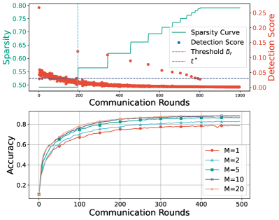
Figure 5: (Top) Relationship between sparsity and detection score; (Bottom) Impact of $M$ involved in each training round on accuracy (CIFAR10, Dir(0.3), $\delta_{pr}=0.03$).

VI-D Ablation Study

VI-D1 Threshold $\delta_{pr}$

Extending total communication rounds from 500 to 1000, we ascertain that a target sparsity of $s=0.8$ is attainable without compromising accuracy (DA-DPFL achieves 89% over DisPFL’s 83.27%). This finding challenges the generalization gap assumption in [11], reducing the need for precise initial sparsity ratio selection in fixed sparsity pruning as DA-DPFL achieves equivalent or lower generalization error at higher sparsity levels through further pruning. Fig.5(Top) shows the pruning decisions based on average detection scores across clients and their sparsity trajectories. The initial high detection score validates the substantial disparity between the random mask and the RigL algorithm-derived mask, differing from EarlyCrop’s centralized, densely initialized model approach. Post $t^{*}$, client models undergo incremental pruning in DA-DPFL, with the pruning scale diminishing due to reduced model compressibility, as evidenced by sparsity alterations at each pruning phase. To ascertain the effect of the early pruning threshold $\delta_{pr}$, we conducted experiments with CIFAR10 and ResNet18. Fig.6 underscores pruning timing significance, indicating varying optimal thresholds for different data partitions and corresponding detection score divergences. Early pruning, though accelerating sparsity achievement, impedes critical learning phases, while excessively delayed pruning equates to post-training pruning, incurring higher costs. Consequently, our results advocate for early-stage further pruning, ideally between 30-40% of total communication rounds, aligning with a threshold range of 0.02-0.03, to balance model performance with energy efficiency.

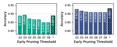
Figure 6: Impact of $\delta_{pr}$ on final prediction accuracy of achieving sparsity $s=0.8$ with CIFAR10 ($M=10$) Dir (left) and Pat (right) partitions (in which * stands for DA-DPFL without further pruning, i.e., fixed sparsity $s=0.5$).

VI-D2 Waiting Threshold $N$

To ensure a fair comparison, we add $N=\{0,2,5\}$ with the same experiment setup as in VI-A for Dir partition. The experimental results in Fig. 7 demonstrate a clear trend: increasing the $N$ consistently improves model accuracy across the CIFAR10 and CIFAR100 datasets, with CIFAR10 seeing up to a 1.87% increase and CIFAR100 a 1.41% increase in accuracy from $N=0$ to $N=10$. Interestingly, the HAM10000 dataset shows no $N=5$ achieves the best performance, suggesting task-specific characteristics influence the optimal selection of $N$. Even the model performance for $N=0$ cases are higher than DisPFL, which illustrates the effectiveness of our further pruning strategy. Furthermore, it is possible to obtain redundancy in reusing models, especially when $M$ is large. By selecting $N$, one can trade off between waiting and model performance.

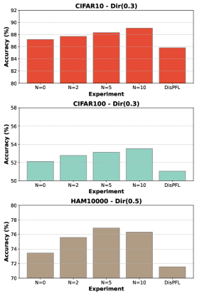
Figure 7: Performance of different number of maximum waiting numbers $N$

VI-E Parallelism and Delay

We conducted $10,000$ iterations to estimate the average impact on parallelism and latency attributed to waiting times. Here, we define parallelism as the proportion of clients that commence training concurrently. The result is depicted in Figures Figure 8 illustrates a decline in parallelism as the number of clients in the neighborhood $M$ increases (having $K=100$ clients). Figure 9 shows delay against $M$. The black line, representing $N=M$, delineates the outcome of awaiting the most delayed clients, i.e., without any control. It is evidenced to scale almost linearly with the neighborhood size $M$. Moreover, in Figure 9, one can observe the efficacy of the constraint $N\leq M$ in mitigating delays while increasing $M$. The mean maximum waiting time is indicative of the multiplier effect on the time required for each communication round relative to traditional decentralized FL. The lines corresponding to $N\in\{1,2,5,10,20\}$ corroborate that the waiting period can be effectively regulated by $N$. In cases where $M=N=100$, DA-DPFL transits to sequential learning, while with $M=100$ and $N=2$, DA-DPFL sustains a comparatively high degree of parallelism with opportunities for model reuse. With $N=0$, DA-DPFL reduces to DisPFL with our pruning strategy.

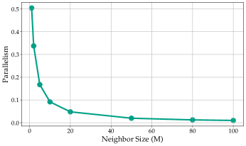
Figure 8: Characteristic of proposed time-varying connected topology: impact on parallelism with different number of neighbor clients.

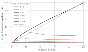
Figure 9: Characteristic of proposed time-varying connected topology: delay induced by waiting with different number of neighbor clients.

VII Conclusions

DA-DPFL is a fair learning scheduling framework that cost-effectively deals with data heterogeneity. DA-DPFL conserves computational & communication resources and accelerates the learning process by introducing a novel sparsity-driven pruning technique. We provide a theoretical analysis on DA-DPFL’s convergence. Comprehensive experiments and comparisons with DFL and CFL baselines in PFL context showcase learning efficiency, enhanced model accuracy, and energy efficiency, which confirms the effectiveness of DA-DPFL in practical applications. DA-DPFL sets the stage for future plans in adaptive algorithms handling time-series and graph data across diverse topologies expanding our models applicability to real-world scenarios.

Additional Algorithms

-A SAP (PQI) Algorithm

In our approach, we adopt the SAP algorithm, as shown in Algorithm 2, to assess the compressibility of neural networks, characterized by four distinct features. Firstly, the initial model employed in our study is inherently sparse. Secondly, we implement PQI pruning as a further pruning technique within a Federated Learning (FL) framework, based on other fixed pruning methodologies. Thirdly, our method incorporates a meticulously designed pruning strategy that ensures proper pruning frequency and specifically avoids further pruning during the critical learning period. Lastly, unlike conventional practices, we integrate the SAP algorithm during the training phase, as opposed to applying it post-training.

Algorithm 2 PQI-driven pruning (Layerwise)

1:  Input: $\tilde{\boldsymbol{\omega}}_{k,E_{l}}^{t}$, mask $\mathbf{m}_{k}^{t}$, norm index $0<p\leq 1<q$, compression hyper-parameter $\eta_{c}$, scaling factor $\gamma$, pruning threshold $\beta$, further pruning time $\mathcal{T}$.

2:  Output: $\tilde{\boldsymbol{\omega}}_{k,E_{l}}^{t\prime}$, corresponding mask $\mathbf{m}_{k}^{t\prime}$

3:  for $t\in\mathcal{T}$ do

4:     for each layer $l\in|L|$ do

5:        Compute dimensionality of $\tilde{\boldsymbol{\omega}}_{k,E_{l}}^{l,t}$: $d_{t}^{l}=|\mathbf{m}_{k}^{l,t}|$

6:        Compute PQ Index $I(\tilde{\boldsymbol{\omega}}_{k,E_{l}}^{l,t})=1-\left(\frac{1}{d_{t}^{l}}\right)^{\frac{1}{q}-\frac{1}{p}}\frac{\|\tilde{\boldsymbol{\omega}}_{k,E_{l}}^{l,t}\|_{p}}{\|\tilde{\boldsymbol{\omega}}_{k,E_{l}}^{l,t}\|_{q}}$

7:        Compute the lower boundary required model parameters to keep $r_{t}^{l}=d_{t}^{l}(1+\eta_{c})^{-\frac{q}{q-p}}\left[1-I(\tilde{\boldsymbol{\omega}}_{k,E_{l}}^{l,t})\right]^{\frac{p}{q-p}}$

8:        Compute the number of model parameters to prune

9:        $c_{t}^{l}=\left\lfloor d_{t}^{l}\cdot\min\left(\gamma\left(1-\frac{r_{t}^{l}}{d_{t}^{l}}\right),\beta\right)\right\rfloor$

10:        Prune $c_{t}^{l}$ model parameters with the smallest magnitude based on $\tilde{\boldsymbol{\omega}}_{k,E_{l}}^{l,t}$ and $\mathbf{m}_{k}^{l,t}$

11:        Find new layer mask $\mathbf{m}_{k}^{l,t\prime}$ and pruned model $\tilde{\boldsymbol{\omega}}_{k,E_{l}}^{l,t\prime}$ at layer $l$

12:     end for

13:     Obtain $\tilde{\boldsymbol{\omega}}_{k,E_{l}}^{t\prime}$ and corresponding mask $\mathbf{m}_{k}^{t\prime}$

14:  end for

-B RigL Algorithm

We follow the RigL algorithm to generate the new mask each communication round, which is shown in Algorithm 3.

Algorithm 3 RigL mask generation

1:  Input: $\tilde{\boldsymbol{\omega}}_{k,E_{l}}^{t\prime}$, corresponding mask $\mathbf{m}_{k}^{t\prime}$, global rounds T, initial annealing ratio $\alpha_{0}$

2:  Output: New mask $\mathbf{m}_{k}^{t+1}$

3:  Compute prune ratio $\alpha_{t}=\frac{\alpha}{2}\left(1+\cos\left(\frac{t\pi}{T}\right)\right)$

4:  Sample one batch of local training data to calculate dense gradient $\mathbf{g}(\tilde{\boldsymbol{\omega}}_{k,E_{l}}^{t\prime})$

5:  for each layer $l\in|L|$ do

6:     Update mask $\mathbf{m}_{k}^{l,t+\frac{1}{2}\prime}$ by pruning $\alpha_{t}$ percentage of weights based on weight magnitude.

7:     Update mask $\mathbf{m}_{k}^{l,t+1}$ via regrowing weights with gradient information $\mathbf{g}(\tilde{\boldsymbol{\omega}}_{k,E_{l}}^{t\prime})$.

8:  end for

9:  Find new mask $\mathbf{m}_{k}^{t+1}$.

Convergence Analysis

In a time-varying connected topology, both $\mathcal{G}_{k}^{t}$ and $\mathcal{N}_{k}^{t}$ are randomly generated. We consider $\mathcal{N}_{k}^{t}=\mathcal{G}_{k}^{t}$ in theoretical analysis since our scheduling policy is regarded as one type of client selection policy.

-C Client Selection Analysis

Given a system with $K$ clients with indices sorted from $1$ to $K$, and considering a particular client with index $k$ then: (1) there are $K-1$ potential clients to select from; (2) among these $K-1$ clients, $k-1$ clients have an index less than $k$; (3) we wish to select $M$ total clients in each sample as client’s $k$ neighbors. Hence, $|\mathcal{N}_{(a)k}|$ is a hypergeometric random variable and the probability $\mathbb{P}(m,k)=\mathbb{P}(|\mathcal{N}_{(a)k}|=m)$ that exactly $m$ of the selected clients have an index less than $k$ is

$$\mathbb{P}(m,k)=\frac{\binom{k-1}{m}\binom{K-k}{M-m}}{\binom{K-1}{M}},$$ (14)

where $\sum_{0\leq m\leq\min_{(M,k-1)}}\mathbb{P}(m,k)=1$, which essentially follows from Vandermonde’s identity.

-D Auxiliary Lemmas and Proofs

DA-DPFL’s local update follows:

$$\tilde{\boldsymbol{\omega}}_{k,\tau+1}^{t}=\tilde{\boldsymbol{\omega}}_{k,\tau}^{t}-\eta\mathbf{g}_{k,\tau}^{t}\odot\mathbf{m}_{k}^{t},$$ (15)

where $\mathbf{g}_{k,\tau}^{t}=\nabla F_{k}(\tilde{\boldsymbol{\omega}}_{k,\tau}^{t})$. This implies that

$$\eta\sum_{\tau=0}^{E_{l}-1}\mathbf{g}_{k,\tau}^{t}\odot\mathbf{m}_{k}^{t}=(\tilde{\boldsymbol{\omega}}_{k,0}^{t}-\tilde{\boldsymbol{\omega}}_{k,E_{l}}^{t})\odot\mathbf{m}_{k}^{t}.$$ (16)

Note that $\boldsymbol{\omega}_{k}^{t+1}=\tilde{\boldsymbol{\omega}}^{t}_{k,E_{l}}$ and $\tilde{\boldsymbol{\omega}}_{k}^{t}=\tilde{\boldsymbol{\omega}}_{k,0}^{t}$. Considering traditional aggregation, like in FedAvg, without scheduling first, we then have Lemma 1.

Lemma 1.

Under Assumptions 1 to 2, for some $M>1$ and $\eta$ such that $\eta^{2}\leq\frac{1}{12M\mu^{2}(M-1)(2M-1)}$,

$$\frac{1}{K}\sum_{k=1}^{K}\mathbb{E}\|\boldsymbol{\omega}_{k}^{t+1}-\tilde{\boldsymbol{\omega}}_{k}^{t}\|^{2}\leq\left(e^{\frac{E_{l}}{2M-2}}-1\right)(2M-2)$$

$$\quad\times\left(\frac{2M}{2M-1}\eta^{2}\sigma^{2}_{l}+6M\eta^{2}(\sigma^{2}_{g}+\sigma^{2}_{p})\right.$$

$$\quad\left.+6M\eta^{2}\frac{\sum_{k=1}^{K}\mathbb{E}\|\nabla f(\tilde{\boldsymbol{\omega}}_{k}^{t})\|^{2}}{K}\right).$$ (17)

Proof.

Because the mask $\mathbf{m}_{k}^{t}$ is consistent during training, we omit the expression with the corresponding model for brevity. We firstly consider the traditional weighted average aggregation where

$$\mathbb{E}\|\tilde{\boldsymbol{\omega}}_{k,\tau+1}^{t}-\tilde{\boldsymbol{\omega}}_{k}^{t}\|^{2}=\mathbb{E}\Big{\|}\tilde{\boldsymbol{\omega}}_{k,\tau}^{t}-\tilde{\boldsymbol{\omega}}_{k}^{t}-\eta\big{(}g_{k,\tau}^{t}\odot\mathbf{m}_{k}^{t}$$

$$\quad-\nabla f_{k}(\tilde{\boldsymbol{\omega}}_{k,\tau}^{t})+\nabla f_{k}(\tilde{\boldsymbol{\omega}}_{k,\tau}^{t})-\nabla f(\tilde{\boldsymbol{\omega}}_{k}^{t})+\nabla f(\tilde{\boldsymbol{\omega}}_{k}^{t})$$

$$\quad-\nabla f_{k}(\tilde{\boldsymbol{\omega}}_{k}^{t})+\nabla f_{k}(\tilde{\boldsymbol{\omega}}_{k}^{t})\big{)}\Big{\|}^{2}.$$ (18)

Write $a:=\mathbb{E}\big{\|}\tilde{\boldsymbol{\omega}}_{k,\tau}^{t}-\eta\big{(}\tilde{g}_{k,\tau}^{t}\odot\mathbf{m}_{k}^{t}-\nabla f_{k}(\tilde{\boldsymbol{\omega}}_{k,\tau}^{t})\big{)}-\tilde{\boldsymbol{\boldsymbol{\omega}}}_{k}^{t}\big{\|}^{2}$ and $b=\eta^{2}\mathbb{E}\|\nabla f_{k}(\tilde{\boldsymbol{\omega}}_{k,\tau}^{t})-\nabla f(\tilde{\boldsymbol{\omega}}_{k}^{t})+\nabla f(\tilde{\boldsymbol{\omega}}_{k}^{t})-\nabla f_{k}(\tilde{\boldsymbol{\omega}}_{k}^{t})+\nabla f_{k}(\tilde{\boldsymbol{\omega}}_{k}^{t})\|^{2}$, using the Cauchy’s inequality with a elastic variable $2M=2M>1$, we have

$$\mathbb{E}\|\boldsymbol{\omega}_{k}^{t+1}-\tilde{\boldsymbol{\omega}}_{k}^{t}\|^{2}\leq(1+\frac{1}{2M-1})a+2Mb.$$ (19)

Then, by Assumptions 1 to 2 and the triangle inequality,

$$a \leq\mathbb{E}\|\tilde{\boldsymbol{\omega}}_{k,\tau}^{t}-\tilde{\boldsymbol{\omega}}_{k}^{t}\|^{2}+\eta^{2}\mathbb{E}\|\tilde{g}_{k,\tau}^{t}\odot\mathbf{m}_{k}^{t}-\nabla f_{k}(\tilde{\boldsymbol{\omega}}_{k,\tau}^{t})\|^{2}$$

$$=\mathbb{E}\|\tilde{\boldsymbol{\omega}}_{k,\tau}^{t}-\tilde{\boldsymbol{\omega}}_{k}^{t}\|^{2}+\eta^{2}\sigma^{2}_{l},$$ (20)

and

$$b \leq 3\eta^{2}\big{[}\mathbb{E}\|\nabla f_{k}(\tilde{\boldsymbol{\omega}}_{k,\tau}^{t})-\nabla f_{k}(\tilde{\boldsymbol{\omega}}_{k}^{t})\|^{2}$$

$$\quad+\mathbb{E}\|\nabla f(\tilde{\boldsymbol{\omega}}_{k}^{t})\|^{2}+\mathbb{E}\|\nabla f_{k}(\tilde{\boldsymbol{\omega}}_{k}^{t})-\nabla f(\tilde{\boldsymbol{\omega}}_{k}^{t})\|^{2}\big{]}$$

$$\leq 3\eta^{2}\big{[}\mathbb{E}\|\nabla f_{k}(\tilde{\boldsymbol{\omega}}_{k,\tau}^{t})-\nabla f_{k}(\tilde{\boldsymbol{\omega}}_{k}^{t})\|^{2}$$

$$\quad+\mathbb{E}\|\nabla f(\tilde{\boldsymbol{\omega}}_{k}^{t})\|^{2}+\mathbb{E}\|\nabla f_{k}(\tilde{\boldsymbol{\omega}}_{k}^{t})-\nabla f(\tilde{\boldsymbol{\omega}}^{t})\|^{2}$$

$$\quad+\mathbb{E}\|\nabla f(\tilde{\boldsymbol{\omega}}_{k}^{t})-\nabla f(\tilde{\boldsymbol{\omega}}^{t})\|^{2}\big{]}$$

$$\leq 3\eta^{2}\big{[}\mu^{2}\mathbb{E}\|\tilde{\boldsymbol{\omega}}_{k,\tau}^{t}-\tilde{\boldsymbol{\omega}}_{k}^{t}\|^{2}+\mathbb{E}\|\nabla f(\tilde{\boldsymbol{\omega}}_{k}^{t})\|^{2}$$

$$\quad+(\sigma^{2}_{g}+\sigma^{2}_{p})\big{]}.$$ (21)

Substitute Eq.(-D) & (-D) into Eq. (19) with some $\eta$ such that $\eta^{2}\leq\frac{1}{12M\mu^{2}(M-1)(2M-1)}$, we have

$$\mathbb{E}\|\tilde{\boldsymbol{\omega}}_{k,\tau+1}^{t}-\tilde{\boldsymbol{\omega}}_{k}^{t}\|^{2}\leq(1+\frac{1}{2M-1}+6M\eta^{2}\mu^{2})\mathbb{E}\|\tilde{\boldsymbol{\omega}}_{k,\tau}^{t}-\tilde{\boldsymbol{\omega}}_{k}^{t}\|^{2}$$

$$\quad+(1+\frac{1}{2M-1})\eta^{2}\sigma^{2}_{l}+6M\eta^{2}(\sigma^{2}_{g}+\sigma^{2}_{p}+\mathbb{E}\|\nabla f(\tilde{\boldsymbol{\omega}}_{k}^{t})\|^{2})$$

$$\leq(1+\frac{1}{2M-2})\mathbb{E}\|\tilde{\boldsymbol{\omega}}_{k,\tau}^{t}-\tilde{\boldsymbol{\omega}}_{k}^{t}\|^{2}$$

$$\quad+(1+\frac{1}{2M-1})\eta^{2}\sigma^{2}_{l}+6M\eta^{2}(\sigma^{2}_{g}+\sigma^{2}_{p}+\mathbb{E}\|\nabla f(\tilde{\boldsymbol{\omega}}_{k}^{t})\|^{2})$$ (22)

Let $A=1+\frac{1}{2(M-1)}$, $B=\left(1+\frac{1}{2M-1}\right)\eta^{2}\sigma^{2}_{l}+6M\eta^{2}(\sigma^{2}_{g}+\sigma^{2}_{p})$, and $C=6M\eta^{2}\mathbb{E}\|\nabla f(\tilde{\boldsymbol{\omega}}_{k}^{t})\|^{2}$, then the recursive inequality Eq.(-D) becomes

$$\mathbb{E}\|\tilde{\boldsymbol{\omega}}_{k,\tau+1}^{t}-\tilde{\boldsymbol{\omega}}_{k}^{t}\|^{2} \leq A\mathbb{E}\|\tilde{\boldsymbol{\omega}}_{k,\tau}^{t}-\tilde{\boldsymbol{\omega}}_{k}^{t}\|^{2}+B+C.$$ (23)

When $\tau=0$, the initial condition is $\mathbb{E}\|\tilde{\boldsymbol{\omega}}_{k,0}^{t}-\tilde{\boldsymbol{\omega}}_{k}^{t}\|^{2}=0$. For $\tau=1$ to $E_{l}$, we apply the inequality Eq.(23) $E_{l}$ times, summing up the constants multiplied by their respective powers of $A$ gives

$$\mathbb{E}\|\tilde{\boldsymbol{\omega}}_{k,E_{l}}^{t}-\tilde{\boldsymbol{\omega}}_{k}^{t}\|^{2} \leq A^{E_{l}}\mathbb{E}\|\tilde{\boldsymbol{\omega}}_{k,0}^{t}-\tilde{\boldsymbol{\omega}}_{k}^{t}\|^{2}+B\sum_{j=0}^{E_{l}-1}A^{j}$$

$$+C\sum_{j=0}^{E_{l}-1}A^{j}.$$ (24)

The sums of the series can be simplified by the sum of a geometric series as follows

$$\sum_{j=0}^{E_{l}-1}A^{j}=\frac{1-A^{E_{l}}}{1-A}.$$ (25)

Hence the inequality can be further simplified as

$$\mathbb{E}\|\tilde{\boldsymbol{\omega}}_{k,E_{l}}^{t}-\tilde{\boldsymbol{\omega}}_{k}^{t}\|^{2} \leq 0+(B+C)\frac{A^{E_{l}}-1}{A-1}.$$ (26)

When $M>1$, $A=1+\frac{1}{2M-2}<e^{\frac{1}{2M-2}}$ hence $A^{E_{l}}<e{{}^{\frac{E_{l}}{2M-2}}}$, which gives the final bound for $\mathbb{E}\|\boldsymbol{\omega}_{k}^{t+1}-\tilde{\boldsymbol{\omega}}_{k}^{t}\|^{2}$ as in Eq.(1). ∎

Lemma 2.

Consider the proposed scheduling strategy. Let $\tilde{\boldsymbol{\omega}}_{k}^{t({\dagger})}$ denote the local personalized aggregated model for the $k$-th client at time $t$. The global aggregated model at time $t$, $\tilde{\boldsymbol{\omega}}^{t({\dagger})}$, is defined as the average of the local models, i.e., $\tilde{\boldsymbol{\omega}}^{t({\dagger})}=\frac{1}{K}\sum_{k=1}^{K}\tilde{\boldsymbol{\omega}}_{k}^{t({\dagger})}$, where $K$ is the total number of clients. Let $M$ represent the number of clients in the neighborhood. With the support of Lemma $1$ in [42], the expected value of the global model at time $t+1$, denoted as $\mathbb{E}(\tilde{\boldsymbol{\omega}}^{t+1({\dagger})})$, is given by

$$\mathbb{E}(\tilde{\boldsymbol{\omega}}^{t+1({\dagger})})=\mathbb{E}(\tilde{\boldsymbol{\omega}}^{t({\dagger})})-\eta\frac{\mathbb{E}\left(\sum_{k=1}^{K}\sum_{\tau=0}^{E_{l}^{*}-1}\mathbf{g}_{\tau,k}(\tilde{\boldsymbol{\omega}}^{t({\dagger})})\right)}{K},$$ (27)

where $E_{l}^{*}=\frac{3M+2}{2(M+1)}E_{l}$, and $E_{l}$ is the number of steps of local updates. Here, $\mathbf{g}_{\tau,k}$ represents the gradient computation for the $k$-th client at local update step $\tau$.

Proof.

Now we consider the effect of DA-DPFL’s scheduling. Rewrite the mask element aggregation with the sequential appointment as

$$\tilde{\boldsymbol{\omega}}_{k}^{t({\dagger})} =\left(\frac{\sum_{j\in\mathcal{N}_{(a)k}^{t}}\boldsymbol{\omega}_{j}^{t}+\sum_{j\in\mathcal{N}_{(b)k}^{t}}\boldsymbol{\omega}_{j}^{t}+\boldsymbol{\omega}_{k}^{t}}{\sum_{j\in\mathcal{N}_{(a)k}^{t}}\mathbf{m}_{j}^{t}+\sum_{j\in\mathcal{N}_{(b)k}^{t}}\mathbf{m}_{j}^{t}+\mathbf{m}_{k}^{t}}\right)\odot\mathbf{m}_{k}^{t}$$ (28)

$$=\left(\frac{\sum_{j\in\mathcal{N}_{(a)k}^{t}}\boldsymbol{\omega}_{j}^{t}+\sum_{j\in\mathcal{N}_{(b)k+}^{t}}\boldsymbol{\omega}_{j}^{t}}{M+1}\right)\odot\mathbf{m}_{k}^{t},$$ (29)

where $\mathcal{N}_{(b)k}^{t}:=\mathcal{N}_{k}^{t}\setminus\mathcal{N}_{(a)k}^{t}$, $\mathcal{N}_{(b)k+}^{t}\coloneqq\mathcal{N}_{(b)k}^{t}\cup\{k\}$, and the last equation holds under Assumption 3.

Similar to Eq.(16), we omit $\mathbf{m}_{k}^{t}$ for convenience on notations since the mask is consistent during local training. Then for the $j$-th client at time $t$, the local personalized aggregated model is

$$\boldsymbol{\omega}_{j}^{t({\dagger})}=\begin{cases}\tilde{\boldsymbol{\omega}}_{j}^{t}-\eta\sum_{\tau=0}^{E_{l}-1}\mathbf{g}_{j,\tau}^{t}\odot\mathbf{m}_{j}^{t},&\text{if }j\in\mathcal{N}_{(a)k}^{t};\\ \boldsymbol{\omega}_{j}^{t},&\text{otherwise}.\end{cases}$$ (30)

When $j\in\mathcal{N}_{(a)k}^{t}$, one can see that $\boldsymbol{\omega}_{j}^{t({\dagger})}$ is equivalent to $\boldsymbol{\omega}_{j}^{t+1}$, reflecting the scenario where, within a single communication round, all participating clients perform an equal number of local training iterations, analogous to traditional FL. The superscript $({\dagger})$ is introduced for an explicit differentiation, signifying that although the local gradients $\mathbf{g}_{j,\tau}^{t}$ are computed under varying aggregation models, they are distinct from those in a synchronous FL framework. Denoted by $I_{\{j\in\mathcal{N}^{t}_{(a)k}\}}$ an indicator function for the event that the $j$-th client is selected in the delayed neighborhoods of client $k$.

Using the results of Proposition 1, it can be shown that

$$\mathbb{E}(\sum_{j\in\mathcal{N}_{(a)k}^{t}}\boldsymbol{\omega}_{j}^{t+1}) =\mathbb{E}(\mathbb{E}(\sum_{j\in\mathcal{N}_{(a)k}^{t}}\boldsymbol{\omega}_{j}^{t+1}||\mathcal{N}^{t}_{(a)k}|))$$

$$=\mathbb{E}(\mathbb{E}(\sum_{j\in\mathcal{N}_{k}^{t}}\boldsymbol{\omega}_{j}^{t+1}I_{\{j\in\mathcal{N}^{t}_{(a)k}\}}||\mathcal{N}^{t}_{(a)k}|))$$

$$=\mathbb{E}(\mathbb{E}(\sum_{j\in\mathcal{N}_{k}^{t}}\boldsymbol{\omega}_{j}^{t+1}I_{\{j\in\mathcal{N}^{t}_{(a)k}||\mathcal{N}^{t}_{(a)k}|\}}))$$

$$=\mathbb{E}(\sum_{j\in\mathcal{N}_{k}^{t}}\boldsymbol{\omega}_{j}^{t+1}\mathbb{E}(I_{\{j\in\mathcal{N}^{t}_{(a)k}||\mathcal{N}^{t}_{(a)k}|\}}))$$

$$=\mathbb{E}(\sum_{j\in\mathcal{N}_{k}^{t}}\boldsymbol{\omega}_{j}^{t+1}\mathbb{P}(j\in\mathcal{N}^{t}_{(a)k}||\mathcal{N}^{t}_{(a)k}|))$$

$$=\mathbb{E}(\sum_{j\in\mathcal{N}_{k}^{t}}\boldsymbol{\omega}_{j}^{t+1}\frac{|\mathcal{N}^{t}_{(a)k}|}{M})$$

$$=\mathbb{E}(|\mathcal{N}^{t}_{(a)k}|)\frac{\mathbb{E}(\sum_{j\in\mathcal{N}_{k}^{t}}\boldsymbol{\omega}_{j}^{t+1})}{M}$$

$$=\frac{(k-1)M}{K-1}\mathbb{E}(\bar{\boldsymbol{\omega}}^{t+1}),$$ (31)

where $|\mathcal{N}^{t}_{(a)k}|$ follows hypergeometric distribution. Similarly,

$$\mathbb{E}(\sum_{j\in\mathcal{N}_{(b)k+}^{t}}\boldsymbol{\omega}_{j}^{t}) =\mathbb{E}(\mathbb{E}(\sum_{j\in\mathcal{N}_{(b)k+}^{t}}\boldsymbol{\omega}_{j}^{t}||\mathcal{N}^{t}_{(b)k+}|))$$

$$=\mathbb{E}(\mathbb{E}(\sum_{j\in\mathcal{N}_{k+}^{t}}\boldsymbol{\omega}_{j}^{t}I_{\{j\in\mathcal{N}^{t}_{(b)k+}\}}||\mathcal{N}^{t}_{(b)k+}|))$$

$$=\mathbb{E}(\mathbb{E}(\sum_{j\in\mathcal{N}_{k+}^{t}}\boldsymbol{\omega}_{j}^{t}I_{\{j\in\mathcal{N}^{t}_{(b)k+}||\mathcal{N}^{t}_{(b)k+}|\}}))$$

$$=\mathbb{E}(\sum_{j\in\mathcal{N}_{k+}^{t}}\boldsymbol{\omega}_{j}^{t}\mathbb{E}(I_{\{j\in\mathcal{N}^{t}_{(b)k+}||\mathcal{N}^{t}_{(b)k+}|\}}))$$

$$=\mathbb{E}(\sum_{j\in\mathcal{N}_{k+}^{t}}\boldsymbol{\omega}_{j}^{t}\mathbb{P}(j\in\mathcal{N}^{t}_{(b)k+}||\mathcal{N}^{t}_{(b)k+}|))$$

$$=\mathbb{E}(\sum_{j\in\mathcal{N}_{k+}^{t}}\boldsymbol{\omega}_{j}^{t}\frac{|\mathcal{N}^{t}_{(b)k+}|-1}{M})$$

$$=\mathbb{E}((|\mathcal{N}^{t}_{(b)k+}|-1))\frac{\mathbb{E}(\sum_{j\in\mathcal{N}_{k+}^{t}}\boldsymbol{\omega}_{j}^{t})}{M}$$

$$=\frac{(K-k)(M+1)}{(K-1)}\mathbb{E}(\bar{\boldsymbol{\omega}}^{t}).$$ (32)

Therefore, $\mathbb{E}(\tilde{\boldsymbol{\omega}}_{k}^{t({\dagger})})$ can be written as

$$[\frac{(k-1)M}{(K-1)(M+1)}\mathbb{E}(\bar{\boldsymbol{\omega}}^{t+1})+\frac{(K-k)}{(K-1)}\mathbb{E}(\bar{\boldsymbol{\omega}}^{t})]\odot\mathbf{m}_{k}^{t}$$

$$=\mathbb{E}(\bar{\boldsymbol{\omega}}^{t})\odot\mathbf{m}_{k}^{t}-[\frac{(k-1)M}{(K-1)(M+1)}\times.$$

$$\quad\mathbb{E}(\frac{\eta\sum_{j\in\mathcal{N}_{k+}^{t}}\sum_{\tau=0}^{E_{l}-1}g_{j,\tau}^{t}}{M+1})]\odot\mathbf{m}_{k}^{t},$$ (33)

where one can verify that when $k=1$, $\mathbb{E}(\tilde{\boldsymbol{\omega}}_{k}^{t({\dagger})})$ reduces to $\mathbb{E}(\tilde{\boldsymbol{\omega}}_{k}^{t})$. Recall that $\tilde{\boldsymbol{\omega}}^{t({\dagger})}=\frac{1}{K}\sum_{k=1}^{K}\tilde{\boldsymbol{\omega}}_{k}^{t({\dagger})}$, then

$$\mathbb{E}(\tilde{\boldsymbol{\omega}}^{t({\dagger})})=\frac{1}{K}\sum_{k=1}^{K}(\mathbb{E}(\bar{\boldsymbol{\omega}}^{t}$$

$$\quad-\frac{(k-1)M}{(K-1)(M+1)}\eta\sum_{j\in\mathcal{N}_{k+}^{t}}\sum_{\tau=0}^{E_{l}-1}g_{j,\tau}^{t}(\bar{\boldsymbol{\omega}}^{t}))\odot\mathbf{m}_{k}^{t})$$

$$=\frac{1}{K}\sum_{k=1}^{K}(\mathbb{E}(\bar{\boldsymbol{\omega}}^{t})-\frac{(k-1)M}{(K-1)(M+1)}\eta\mathbb{E}(\tilde{g}_{k}^{t})\odot\mathbf{m}_{k}^{t})$$ (34)

$$=\mathbb{E}(\bar{\boldsymbol{\omega}}^{t})-\frac{1}{K}\sum_{k=1}^{K}(\frac{(k-1)M}{(K-1)(M+1)}\eta\mathbb{E}(\tilde{g}_{k}^{t}))\odot\mathbf{m}_{k}^{t},$$ (35)

where $\tilde{g}_{k}^{t}=\frac{\sum_{j\in\mathcal{N}_{k+}^{t}}\sum_{\tau=0}^{E_{l}-1}g_{j,\tau}^{t}}{M+1}$ and the last equality holds according to the definition of $\bar{\boldsymbol{\omega}}^{t}$. $g_{j,\tau}^{t}(\bar{\boldsymbol{\omega}})$ means the gradient at local epoch $\tau=0$ is with respect to $\bar{\boldsymbol{\omega}}$. Let $\tilde{g}^{t({\dagger})}=\frac{1}{K}\sum_{k=1}^{K}[\frac{(k-1)M}{(K-1)(M+1)}\tilde{g}_{k}^{t}\odot\mathbf{m}_{k}^{t}]$, then

$$\mathbb{E}(\tilde{\boldsymbol{\omega}}^{t({\dagger})}) =\mathbb{E}(\bar{\boldsymbol{\omega}}^{t})-\eta\mathbb{E}(\tilde{g}^{t({\dagger})}).$$ (36)

To find the boundary for the difference between the global model at time $t$ and $t+1$ and according to Assumption 1, we have

$$\mathbb{E}[f(\tilde{\boldsymbol{\omega}}^{t+1({\dagger})})]-\mathbb{E}[f(\tilde{\boldsymbol{\omega}}^{t({\dagger})})]$$

$$\leq\mathbb{E}\left[\left<f(\nabla\tilde{\boldsymbol{\omega}}^{t({\dagger})}),\tilde{\boldsymbol{\omega}}^{t+1({\dagger})}-\tilde{\boldsymbol{\omega}}^{t({\dagger})}\right>\right]$$

$$\quad+\frac{\mu}{2}\|\tilde{\boldsymbol{\omega}}^{t+1({\dagger})}-\tilde{\boldsymbol{\omega}}^{t({\dagger})}\|^{2}.$$ (37)

Lemma $1$ in [42] ensures that $\forall k\in\lvert K\rvert,\ \mathbb{E}\left(\frac{\sum_{k=1}^{K}\sum_{\tau=0}^{E_{l}-1}\mathbf{g}_{\tau,k}(\tilde{\boldsymbol{\omega}}^{t({\dagger})})}{K}\right)=\mathbb{E}[\mathbf{\tilde{g}}_{k}^{t}]$ since $\mathcal{N}_{k}^{t}$ is selected randomly. According to the definition and Eq. (36),

$$\mathbb{E}(\tilde{\boldsymbol{\omega}}^{t+1({\dagger})}) =\mathbb{E}(\bar{\boldsymbol{\omega}}^{t+1})-\eta\mathbb{E}(\tilde{g}^{t+1({\dagger})})$$

$$=\mathbb{E}(\tilde{\boldsymbol{\omega}}^{t({\dagger})})-\eta\frac{\mathbb{E}\left(\sum_{k=1}^{K}\sum_{\tau=0}^{E_{l}-1}\mathbf{g}_{\tau,k}(\tilde{\boldsymbol{\omega}}^{t({\dagger})})\right)}{K}$$

$$\quad-\eta\mathbb{E}(\tilde{g}^{t+1({\dagger})})$$ (38)

$$=\mathbb{E}(\tilde{\boldsymbol{\omega}}^{t({\dagger})})-\eta\frac{\mathbb{E}\left(\sum_{k=1}^{K}\sum_{\tau=0}^{E_{l}^{*}-1}\mathbf{g}_{\tau,k}(\tilde{\boldsymbol{\omega}}^{t({\dagger})})\right)}{K},$$ (39)

where $E_{l}^{*}=E_{l}+\frac{M}{2(M+1)}E_{l}$. Actually, here the starting weights of $\tilde{g}^{t+1({\dagger})}$ is with respect to $\mathbb{E}(\bar{\boldsymbol{\omega}}^{t+1})=\ \mathbb{E}(\tilde{\boldsymbol{\omega}}^{t({\dagger})})-\eta\frac{\sum_{k=1}^{K}\mathbb{E}\sum_{\tau=0}^{E_{l}-1}\left(\mathbf{g}_{\tau,k}(\tilde{\boldsymbol{\omega}}^{t({\dagger})})\right)}{K}$. One can think of just continuing $\frac{M}{2(M+1)}$ more steps of local training, where $\frac{1}{K}\sum_{k=1}^{K}[\frac{(k-1)M}{(K-1)(M+1)}]=\frac{M}{2(M+1)}$. $E_{l}^{*}$ might not be an integer, we just use this to conclude the effect of sequential aligning for convergence analysis. ∎

Now, the target is to prove the boundary of $\mathbb{E}<f(\nabla\tilde{\boldsymbol{\omega}}^{t({\dagger})}),\tilde{\boldsymbol{\omega}}^{t+1({\dagger})}-\tilde{\boldsymbol{\omega}}^{t({\dagger})}>$ and $\frac{\mu}{2}\|\tilde{\boldsymbol{\omega}}^{t+1({\dagger})}-\tilde{\boldsymbol{\omega}}^{t({\dagger})}\|^{2}$.

Lemma 3.

Under Assumptions 1 to 2 and Lemma 2, suppose $\tilde{\boldsymbol{\omega}}^{t+1({\dagger})}$ and $\tilde{\boldsymbol{\omega}}^{t({\dagger})}$ are global model learned by the proposed strategy, for some $M>1$ with $\eta\leq\sqrt{\frac{1}{12M\mu^{2}(M-1)(2M-1)}}$, $\mathbb{E}\left[\frac{\mu}{2}\|\tilde{\boldsymbol{\omega}}^{t+1({\dagger})}-\tilde{\boldsymbol{\omega}}^{t({\dagger})}\|^{2}\right]$ is upper bounded by

$$\mathbb{E}\left[\frac{\mu}{2}\|\tilde{\boldsymbol{\omega}}^{t+1({\dagger})}-\tilde{\boldsymbol{\omega}}^{t({\dagger})}\|^{2}\right]\leq\mu S_{1}(S_{2}+3\mathbb{E}\|\nabla f(\tilde{\boldsymbol{\omega}}^{t({\dagger})}\|^{2}),$$

where $S_{1}=2\eta^{2}M(M-1)\left(\exp{\left(\frac{(3M+2)E_{l}}{4(M^{2}-1)}\right)}-1\right)$ and $S_{2}=\frac{1}{2M-1}\sigma^{2}_{l}+3(\sigma^{2}_{g}+2\sigma^{2}_{p})$.

Proof.

Lemma 1 states the boundary for the local updates. Eq. (-D) and Lemma 2 states that the scheduling increases the local epochs $E_{l}$ to $E_{l}^{*}$ with the expectation for the (aggregated) global model. Hence,

$$\mathbb{E} \left[\|\tilde{\boldsymbol{\omega}}^{t+1({\dagger})}-\tilde{\boldsymbol{\omega}}^{t({\dagger})}\|^{2}\right]$$

$$=\mathbb{E}\left[\|\frac{1}{K}\sum_{k=1}^{K}\tilde{\boldsymbol{\omega}}_{k}^{t+1({\dagger})}-\frac{1}{K}\sum_{k=1}^{K}\tilde{\boldsymbol{\omega}}_{k}^{t({\dagger})}\|^{2}\right]$$

$$\leq\mathbb{E}\left[\frac{1}{K}\sum_{k=1}^{K}\|\tilde{\boldsymbol{\omega}}_{k}^{t+1({\dagger})}-\tilde{\boldsymbol{\omega}}_{k}^{t({\dagger})}\|^{2}\right].$$ (40)

The last inequality holds since Jensen’s Inequality where the defined function $\phi(.)=\|.\|^{2}$ is convex. Therefore, substituting the results of Lemma 1 and changing $E_{l}$ by $E_{l}^{*}+1$, we have a boundary with $\frac{\sum_{k=1}^{K}\mathbb{E}\|\nabla f(\tilde{\boldsymbol{\omega}}_{k}^{t({\dagger})})\|^{2}}{K}$. With the triangle inequality again and Assumption 2,

$$\frac{\sum_{k=1}^{K}\mathbb{E}\|\nabla f(\tilde{\boldsymbol{\omega}}_{k}^{t({\dagger})})\|^{2}}{K}$$

$$=\frac{\sum_{k=1}^{K}\mathbb{E}\|\nabla f(\tilde{\boldsymbol{\omega}}_{k}^{t({\dagger})})-\nabla f(\tilde{\boldsymbol{\omega}}^{t({\dagger})})+\nabla f(\tilde{\boldsymbol{\omega}}^{t({\dagger})})\|^{2}}{K}$$

$$\leq\frac{\sum_{k=1}^{K}\mathbb{E}\|\nabla f(\tilde{\boldsymbol{\omega}}_{k}^{t({\dagger})})-\nabla f(\tilde{\boldsymbol{\omega}}^{t({\dagger})})\|^{2}+\|\nabla f(\tilde{\boldsymbol{\omega}}^{t({\dagger})})\|^{2}}{K}$$

$$\leq\mathbb{E}\|\nabla f(\tilde{\boldsymbol{\omega}}^{t({\dagger})}\|^{2}+\sigma_{p}^{2},$$ (41)

which finishes the proof. ∎

Lemma 4.

Under Assumptions 1 to 2 and Lemma 3, $\mathbb{E}\left[<\nabla f(\tilde{\boldsymbol{\omega}}^{t({\dagger})}),\tilde{\boldsymbol{\omega}}^{t+1({\dagger})}-\tilde{\boldsymbol{\omega}}^{t({\dagger})}>\right]$ is upper bounded by

$$-\frac{\eta}{2}\|\nabla f(\tilde{\boldsymbol{\omega}}^{t({\dagger})})\|^{2}-\frac{\eta}{2}\mathbb{E}\|\hat{\mathbf{g}}^{t({\dagger})}\|^{2}+\frac{3\mu^{2}\eta^{3}E_{l}^{*}}{M}(\sigma_{l}^{2}+\sigma_{g}^{2})$$ (42)

where $E_{l}^{*}=\frac{3M+2}{2(M+1)}E_{l}$

Proof.

According to Eq. (-D) and let $\hat{\mathbf{g}}^{t({\dagger})}=\frac{\sum_{k=1}^{K}\sum_{\tau=0}^{E_{l}^{*}}\mathbf{g}_{\tau,k}(\tilde{\boldsymbol{\omega}}^{t({\dagger})})}{K}$,

$\mathbb{E}[<\nabla f(\tilde{\boldsymbol{\omega}}^{t({\dagger})}),\tilde{\boldsymbol{\omega}}^{t+1({\dagger})}-\tilde{\boldsymbol{\omega}}^{t({\dagger})}>]=-\eta\mathbb{E}\left[<\nabla f(\tilde{\boldsymbol{\omega}}^{t({\dagger})}),\mathbb{E}\left(\hat{\mathbf{g}}^{t({\dagger})}\right)>\right]$. Let’s prove the boundary for $-\mathbb{E}\left[<\nabla f(\tilde{\boldsymbol{\omega}}^{t({\dagger})}),\mathbb{E}\left(\hat{\mathbf{g}}^{t({\dagger})}\right)>\right]$.

$$-\mathbb{E}[\left<\nabla f(\tilde{\boldsymbol{\omega}}^{t({\dagger})}),\mathbb{E}\left(\hat{\mathbf{g}}^{t({\dagger})}\right)\right>]\stackrel{{\scriptstyle(a)}}{{=}}-\frac{1}{2}\|\nabla f(\tilde{\boldsymbol{\omega}}^{t({\dagger})})\|^{2}$$

$$-\frac{1}{2}\mathbb{E}\|\hat{\mathbf{g}}^{t({\dagger})}\|^{2}+\frac{1}{2}\|\nabla f(\tilde{\boldsymbol{\omega}}^{t({\dagger})})-\mathbb{E}[\hat{\mathbf{g}}^{t({\dagger})}]\|^{2}$$ (43)

, where $(a)$ is due to $<\mathbf{a},\mathbf{b}>=\frac{\mathbf{a}^{2}+\mathbf{b}^{2}-(\mathbf{a}-\mathbf{b})^{2}}{2}$. Then only the third term in the right-hand-side is left, since the boundary for the first and second term can be found by Lemma 3. Based on Assumption 1 and denote $t_{c}$ as the start of the communication round of $t$, i.e before training,

$$\frac{1}{2}\|\nabla f(\tilde{\boldsymbol{\omega}}^{t({\dagger})})-\mathbb{E}[\hat{\mathbf{g}}^{t({\dagger})}]\|^{2}\leq\frac{\mu^{2}}{2K}\sum_{k=1}^{K}\mathbb{E}\|\tilde{\boldsymbol{\omega}}^{t({\dagger})}-\tilde{\boldsymbol{\omega}}^{t({\dagger})}_{k}\|^{2}$$

$$=\frac{\mu^{2}}{2}\sum_{k=1}^{K}\mathbb{E}[\frac{1}{K}\|\tilde{\boldsymbol{\omega}}^{t_{c}({\dagger})}-\frac{1}{K}\sum_{j=1}^{K}\mathbb{E}_{\mathcal{P}_{t,j}}[\frac{\eta}{M}\sum_{j\in\mathcal{P}_{t,j}}\sum_{\tau=t_{c}}^{t_{c}+E_{l}^{*}}\tilde{g}_{\tau,j}^{t_{c}({\dagger})}]$$

$$\quad-\tilde{\boldsymbol{\omega}}^{t_{c}({\dagger})}+\mathbb{E}_{\mathcal{P}_{t,k}}[\frac{\eta}{M}\sum_{k\in\mathcal{P}_{t,k}}\sum_{\tau=t_{c}}^{t_{c}+E_{l}^{*}}\tilde{g}_{\tau,k}^{t_{c}({\dagger})}]\|^{2}]$$

$$=\frac{\mu^{2}\eta^{2}}{2}\sum_{k=1}^{K}\mathbb{E}[\frac{1}{K}\|\mathbb{E}_{\mathcal{P}_{t,k}}[\frac{1}{M}\sum_{k\in\mathcal{P}_{t,k}}\sum_{\tau=t_{c}}^{t_{c}+E_{l}^{*}}\tilde{g}_{\tau,k}^{t_{c}({\dagger})}]$$

$$\quad-\frac{1}{K}\sum_{j=1}^{K}\mathbb{E}_{\mathcal{P}_{t,j}}[\frac{1}{M}\sum_{j\in\mathcal{P}_{t,j}}\sum_{\tau=t_{c}}^{t_{c}+E_{l}^{*}}\tilde{g}_{\tau,j}^{t_{c}({\dagger})}]\|^{2}]$$

$$=\frac{\mu^{2}\eta^{2}}{2}\sum_{k=1}^{K}\mathbb{E}[\frac{1}{K}\|\mathbb{E}_{\mathcal{P}_{t,k}}[\frac{1}{M}\sum_{k\in\mathcal{P}_{t,k}}\sum_{\tau=t_{c}}^{t_{c}+E_{l}^{*}}(\tilde{g}_{\tau,k}^{t_{c}({\dagger})}-\nabla f_{k}(\tilde{\boldsymbol{\omega}}^{t_{c}({\dagger})}_{k,\tau}))]$$

$$\quad-\frac{1}{K}\sum_{j=1}^{K}\mathbb{E}_{\mathcal{P}_{t,j}}[\frac{1}{M}\sum_{j\in\mathcal{P}_{t,j}}\sum_{\tau=t_{c}}^{t_{c}+E_{l}^{*}}(\tilde{g}_{\tau,j}^{t_{c}({\dagger})}-\nabla f_{j}(\tilde{\boldsymbol{\omega}}^{t_{c}({\dagger})}_{j,\tau}))]$$

$$\quad+\mathbb{E}_{\mathcal{P}_{t,k}}[\frac{1}{M}\sum_{k\in\mathcal{P}_{t,k}}\sum_{\tau=t_{c}}^{t_{c}+E_{l}^{*}}\nabla f_{k}(\tilde{\boldsymbol{\omega}}^{t_{c}({\dagger})}_{k,\tau})]$$

$$\quad-\frac{1}{K}\sum_{j=1}^{K}\mathbb{E}_{\mathcal{P}_{t,j}}[\frac{1}{M}\sum_{j\in\mathcal{P}_{t,j}}\sum_{\tau=t_{c}}^{t_{c}+E_{l}^{*}}\nabla f_{j}(\tilde{\boldsymbol{\omega}}^{t_{c}({\dagger})}_{j,\tau})]\|^{2}].$$

$$\stackrel{{\scriptstyle(b)}}{{\leq}}\frac{3\mu^{2}\eta^{2}}{2K}\sum_{k=1}^{K}[\mathbb{E}_{\mathcal{P}_{t,j}}\|\frac{1}{M}\sum_{k\in\mathcal{P}_{t,k}}\sum_{\tau=t_{c}}^{t_{c}+E_{l}^{*}}(\tilde{g}_{\tau,k}^{t_{c}({\dagger})}$$

$$\qquad-\nabla f_{k}(\tilde{\boldsymbol{\omega}}^{t_{c}({\dagger})}_{k,\tau}))\|^{2}$$

$$\quad+\frac{1}{K}\sum_{j=1}^{K}\mathbb{E}_{\mathcal{P}_{t,j}}[\|\frac{1}{M}\sum_{j\in\mathcal{P}_{t,j}}\sum_{\tau=t_{c}}^{t_{c}+E_{l}^{*}}\nabla f_{j}(\tilde{\boldsymbol{\omega}}^{t_{c}({\dagger})}_{j,\tau})\|^{2}]$$

$$\quad+.\|\mathbb{E}_{\mathcal{P}_{t,k}}[\frac{1}{M}\sum_{k\in\mathcal{P}_{t,k}}\sum_{\tau=t_{c}}^{t_{c}+E_{l}^{*}}\nabla f_{k}(\tilde{\boldsymbol{\omega}}^{t_{c}({\dagger})}_{k,\tau})]$$

$$\qquad-\frac{1}{K}\sum_{j=1}^{K}\mathbb{E}_{\mathcal{P}_{t,j}}[\frac{1}{M}\sum_{j\in\mathcal{P}_{t,j}}\sum_{\tau=t_{c}}^{t_{c}+E_{l}^{*}}\nabla f_{j}(\tilde{\boldsymbol{\omega}}^{t_{c}({\dagger})}_{j,\tau})]\|^{2}]]$$

$$\stackrel{{\scriptstyle(c)}}{{\leq}}\frac{3\mu^{2}\eta^{2}}{2K}[\frac{E_{l}^{*}}{M}\sigma_{l}^{2}+\frac{E_{l}^{*}K\sigma^{2}_{l}}{KM}+\frac{E_{l}^{*}}{M}\sigma_{g}^{2}+\frac{E_{l}^{*}K\sigma^{2}_{g}}{KM}]$$

$$=\frac{3\mu^{2}\eta^{2}E_{l}^{*}}{M}(\sigma_{l}^{2}+\sigma_{g}^{2})$$ (44)

In the above formulation, the variable $j$ serves to distinguish from $k$, ensuring clarity in the representation of individual client contributions. Here, $\mathcal{P}_{t,k}$ denotes the selection probability of client $k$ at time $t$. The inequality marked as $(b)$ derives from the application of the Cauchy-Schwarz inequality, exemplified by the relation $\|a+b+c\|^{2}\leq 3(\|a\|^{2}+\|b\|^{2}+\|c\|^{2})$. The step labeled as $(c)$ leverages a similar analytical technique, focusing on the aggregation of global gradients, thereby facilitating the derivation of $\sigma^{2}_{g}$, which is in conjunction with Assumption 2. Substitute the results from Lemma 3 to Eq.(-D) with multiplying $\eta$ to conclude the proof for Lemma 4.

∎

-E Proof for Theorem 1

Combining the bounds from Lemma 3 and Lemma 4, we have:

$$\mathbb{E}[f(\tilde{\boldsymbol{\omega}}^{t+1({\dagger})})]-\mathbb{E}[f(\tilde{\boldsymbol{\omega}}^{t({\dagger})})]\leq$$

$$\quad\mathbb{E}[\frac{\mu}{2}\|\tilde{\boldsymbol{\omega}}^{t+1({\dagger})}-\tilde{\boldsymbol{\omega}}^{t({\dagger})}\|^{2}]$$ (45)

$$+\mathbb{E}[\langle\nabla f(\tilde{\boldsymbol{\omega}}^{t({\dagger})}),\tilde{\boldsymbol{\omega}}^{t+1({\dagger})}-\tilde{\boldsymbol{\omega}}^{t({\dagger})}\rangle]$$

$$=-\frac{\eta}{2}\|\nabla f(\tilde{\boldsymbol{\omega}}^{t({\dagger})})\|^{2}+\frac{\mu-\eta}{2}\mathbb{E}\|\hat{\mathbf{g}}^{t({\dagger})}\|^{2}+\frac{3\mu^{2}\eta^{3}E_{l}^{*}}{M}(\sigma_{l}^{2}+\sigma_{g}^{2})$$ (46)

$$\leq\frac{6S_{1}(\mu-\eta)-\eta}{2}\|\nabla f(\tilde{\boldsymbol{\omega}}^{t({\dagger})})\|^{2}+(\mu-\eta)S_{1}S_{2}+$$

$$\quad\frac{3\mu^{2}\eta^{3}(\frac{3M+2}{2(M+1)}E_{l}-1)}{M}(\sigma_{l}^{2}+\sigma_{g}^{2}).$$ (47)

It is the fact that $\min{\|\nabla f(\tilde{\boldsymbol{\omega}}^{t({\dagger})}\|^{2}}\leq\frac{\sum_{t=0}^{T-1}\|\nabla f(\tilde{\boldsymbol{\omega}}^{t({\dagger})}\|^{2}}{T}$. Summing up Eq. (-E) from $t=0$ to a large $t=T$ concludes the proof. In detail, Given the inequality for each iteration $t$:

$$\mathbb{E}[f(\tilde{\boldsymbol{\omega}}^{t+1({\dagger})})]-\mathbb{E}[f(\tilde{\boldsymbol{\omega}}^{t({\dagger})})]\leq\frac{6S_{1}(\mu-\eta)-\eta}{2}\|\nabla f(\tilde{\boldsymbol{\omega}}^{t({\dagger})})\|^{2}$$ (48)

$$+(\mu-\eta)S_{1}S_{2}+\frac{3\mu^{2}\eta^{3}\left(\frac{3M+2}{2(M+1)}E_{l}-1\right)}{M}(\sigma_{l}^{2}+\sigma_{g}^{2}).$$

Summing this inequality from $t=0$ to $t=T-1$ yields:

$$\mathbb{E}[f(\tilde{\boldsymbol{\omega}}^{T({\dagger})})]-\mathbb{E}[f(\tilde{\boldsymbol{\omega}}^{0({\dagger})})]$$ (49)

$$\leq\sum_{t=0}^{T-1}\left(\frac{6S_{1}(\mu-\eta)-\eta}{2}\|\nabla f(\tilde{\boldsymbol{\omega}}^{t({\dagger})})\|^{2}\right)+T\cdot\left[(\mu-\eta)S_{1}S_{2}\right.$$

$$\quad\left.+\frac{3\mu^{2}\eta^{3}\left(\frac{3M+2}{2(M+1)}E_{l}-1\right)}{M}(\sigma_{l}^{2}+\sigma_{g}^{2})\right].$$

To isolate the cumulative gradient norm terms across $T$ iterations, we divide the inequality by the coefficient of the gradient norm term:

$$\sum_{t=0}^{T-1}\|\nabla f( \tilde{\boldsymbol{\omega}}^{t({\dagger})})\|^{2}$$ (50)

$$\leq\frac{2}{\eta-6S_{1}(\mu-\eta)}\left(\mathbb{E}[f(\tilde{\boldsymbol{\omega}}^{0({\dagger})})]-\mathbb{E}[f(\tilde{\boldsymbol{\omega}}^{T({\dagger})})]\right)$$

$$\quad+S_{3}T$$

, where $S_{3}=\frac{2}{\eta-6S_{1}(\mu-\eta)}\cdot\left[(\mu-\eta)S_{1}S_{2}+\frac{3\mu^{2}\eta^{3}(3M+2)E_{l}}{2(M+1)M}(\sigma_{l}^{2}+\sigma_{g}^{2})\right]$. When T is large, The denominator $\eta-6S_{1}(\mu-\eta)$ is nominated by $\eta$. Then when we choose $\eta\propto\mathcal{O}(\frac{1}{\sqrt{T}\mu})$ and as $T$ is large enough, $S_{3}$ diminishes closely to $0$.

References

• [1] X. Zhai, A. Kolesnikov, N. Houlsby, and L. Beyer, “Scaling vision transformers,” in Proceedings of the IEEE/CVF Conference on Computer Vision and Pattern Recognition, 2022, pp. 12 104–12 113.
• [2] J. Deng, W. Dong, R. Socher, L.-J. Li, K. Li, and L. Fei-Fei, “Imagenet: A large-scale hierarchical image database,” in 2009 IEEE conference on computer vision and pattern recognition.   Ieee, 2009, pp. 248–255.
• [3] B. McMahan, E. Moore, D. Ramage, S. Hampson, and B. A. y Arcas, “Communication-efficient learning of deep networks from decentralized data,” in Artificial intelligence and statistics.   PMLR, 2017, pp. 1273–1282.
• [4] Q. Li, Z. Wen, Z. Wu, S. Hu, N. Wang, Y. Li, X. Liu, and B. He, “A survey on federated learning systems: vision, hype and reality for data privacy and protection,” IEEE Trans Knowl Data Eng, 2021.
• [5] T. Li, A. K. Sahu, A. Talwalkar, and V. Smith, “Federated learning: Challenges, methods, and future directions,” IEEE signal processing magazine, vol. 37, no. 3, pp. 50–60, 2020.
• [6] J. Sun, T. Chen, G. Giannakis, and Z. Yang, “Communication-efficient distributed learning via lazily aggregated quantized gradients,” Advances in Neural Information Processing Systems, vol. 32, 2019.
• [7] Y. Lin, S. Han, H. Mao, Y. Wang, and B. Dally, “Deep gradient compression: Reducing the communication bandwidth for distributed training,” in International Conference on Learning Representations, 2018.
• [8] Y. Jiang, S. Wang, V. Valls, B. J. Ko, W.-H. Lee, K. K. Leung, and L. Tassiulas, “Model pruning enables efficient federated learning on edge devices,” IEEE Transactions on Neural Networks and Learning Systems, 2022.
• [9] B. Isik, F. Pase, D. Gunduz, T. Weissman, and Z. Michele, “Sparse random networks for communication-efficient federated learning,” in The Eleventh International Conference on Learning Representations, 2023.
• [10] Q. Long, C. Anagnostopoulos, S. P. Parambath, and D. Bi, “Feddip: Federated learning with extreme dynamic pruning and incremental regularization,” in 2023 IEEE International Conference on Data Mining (ICDM).   IEEE, 2023, pp. 1187–1192.
• [11] R. Dai, L. Shen, F. He, X. Tian, and D. Tao, “Dispfl: Towards communication-efficient personalized federated learning via decentralized sparse training,” in International Conference on Machine Learning.   PMLR, 2022, pp. 4587–4604.
• [12] A. Li, J. Sun, X. Zeng, M. Zhang, H. Li, and Y. Chen, “Fedmask: Joint computation and communication-efficient personalized federated learning via heterogeneous masking,” in Proceedings of the 19th ACM Conference on Embedded Networked Sensor Systems, 2021, pp. 42–55.
• [13] M. Zhang, K. Sapra, S. Fidler, S. Yeung, and J. M. Alvarez, “Personalized federated learning with first order model optimization,” in International Conference on Learning Representations, 2021.
• [14] T. Li, S. Hu, A. Beirami, and V. Smith, “Ditto: Fair and robust federated learning through personalization,” in International Conference on Machine Learning.   PMLR, 2021, pp. 6357–6368.
• [15] T. Huang, S. Liu, L. Shen, F. He, W. Lin, and D. Tao, “Achieving personalized federated learning with sparse local models,” arXiv preprint arXiv:2201.11380, 2022.
• [16] D. Wang, L. Shen, Y. Luo, H. Hu, K. Su, Y. Wen, and D. Tao, “Fedabc: targeting fair competition in personalized federated learning,” in Proceedings of the Thirty-Seventh AAAI Conference on Artificial Intelligence and Thirty-Fifth Conference on Innovative Applications of Artificial Intelligence and Thirteenth Symposium on Educational Advances in Artificial Intelligence, ser. AAAI’23/IAAI’23/EAAI’23.   AAAI Press, 2023. [Online]. Available: https://doi.org/10.1609/aaai.v37i8.26203
• [17] T. Huang, L. Shen, Y. Sun, W. Lin, and D. Tao, “Fusion of global and local knowledge for personalized federated learning,” Transactions on Machine Learning Research, 2022.
• [18] L. Yuan, L. Sun, P. S. Yu, and Z. Wang, “Decentralized federated learning: A survey and perspective,” arXiv preprint arXiv:2306.01603, 2023.
• [19] T. Sun, D. Li, and B. Wang, “Decentralized federated averaging,” IEEE Transactions on Pattern Analysis and Machine Intelligence, vol. 45, no. 4, pp. 4289–4301, 2022.
• [20] H. Zhao, B. Li, Z. Li, P. Richtárik, and Y. Chi, “Beer: Fast $o(1/t)$ rate for decentralized nonconvex optimization with communication compression,” Advances in Neural Information Processing Systems, vol. 35, pp. 31 653–31 667, 2022.
• [21] C.-Y. Yau and H. T. Wai, “Docom: Compressed decentralized optimization with near-optimal sample complexity,” Transactions on Machine Learning Research, 2023.
• [22] S. Bibikar, H. Vikalo, Z. Wang, and X. Chen, “Federated dynamic sparse training: Computing less, communicating less, yet learning better,” in Proceedings of the AAAI Conference on Artificial Intelligence, vol. 36, no. 6, 2022, pp. 6080–6088.
• [23] D. Chen, L. Yao, D. Gao, B. Ding, and Y. Li, “Efficient personalized federated learning via sparse model-adaptation,” in Proceedings of the 40th International Conference on Machine Learning, ser. Proceedings of Machine Learning Research, A. Krause, E. Brunskill, K. Cho, B. Engelhardt, S. Sabato, and J. Scarlett, Eds., vol. 202.   PMLR, 23–29 Jul 2023, pp. 5234–5256. [Online]. Available: https://proceedings.mlr.press/v202/chen23aj.html
• [24] A. Lalitha, S. Shekhar, T. Javidi, and F. Koushanfar, “Fully decentralized federated learning,” in Third workshop on bayesian deep learning (NeurIPS), vol. 2, 2018.
• [25] Z. Tang, S. Shi, B. Li, and X. Chu, “Gossipfl: A decentralized federated learning framework with sparsified and adaptive communication,” IEEE Transactions on Parallel and Distributed Systems, vol. 34, no. 3, pp. 909–922, 2022.
• [26] Y. Shi, L. Shen, K. Wei, Y. Sun, B. Yuan, X. Wang, and D. Tao, “Improving the model consistency of decentralized federated learning,” in Proceedings of the 40th International Conference on Machine Learning, ser. Proceedings of Machine Learning Research, A. Krause, E. Brunskill, K. Cho, B. Engelhardt, S. Sabato, and J. Scarlett, Eds., vol. 202.   PMLR, 23–29 Jul 2023, pp. 31 269–31 291. [Online]. Available: https://proceedings.mlr.press/v202/shi23d.html
• [27] J. Frankle, G. K. Dziugaite, D. Roy, and M. Carbin, “Linear mode connectivity and the lottery ticket hypothesis,” in International Conference on Machine Learning.   PMLR, 2020, pp. 3259–3269.
• [28] J. Rachwan, D. Zügner, B. Charpentier, S. Geisler, M. Ayle, and S. Günnemann, “Winning the lottery ahead of time: Efficient early network pruning,” in Proceedings of the 39th International Conference on Machine Learning, ser. Proceedings of Machine Learning Research, K. Chaudhuri, S. Jegelka, L. Song, C. Szepesvari, G. Niu, and S. Sabato, Eds., vol. 162.   PMLR, 17–23 Jul 2022, pp. 18 293–18 309. [Online]. Available: https://proceedings.mlr.press/v162/rachwan22a.html
• [29] T. Hoefler, D. Alistarh, T. Ben-Nun, N. Dryden, and A. Peste, “Sparsity in deep learning: Pruning and growth for efficient inference and training in neural networks,” Journal of Machine Learning Research, vol. 22, no. 241, pp. 1–124, 2021.
• [30] U. Evci, T. Gale, J. Menick, P. S. Castro, and E. Elsen, “Rigging the lottery: Making all tickets winners,” in International Conference on Machine Learning.   PMLR, 2020, pp. 2943–2952.
• [31] E. Diao, G. Wang, J. Zhang, Y. Yang, J. Ding, and V. Tarokh, “Pruning deep neural networks from a sparsity perspective,” in The Eleventh International Conference on Learning Representations, 2022.
• [32] G. Yan, H. Wang, X. Yuan, and J. Li, “Criticalfl: A critical learning periods augmented client selection framework for efficient federated learning,” in Proceedings of the 29th ACM SIGKDD Conference on Knowledge Discovery and Data Mining, 2023, pp. 2898–2907.
• [33] S. Jastrzebski, D. Arpit, O. Astrand, G. B. Kerg, H. Wang, C. Xiong, R. Socher, K. Cho, and K. J. Geras, “Catastrophic fisher explosion: Early phase fisher matrix impacts generalization,” in International Conference on Machine Learning.   PMLR, 2021, pp. 4772–4784.
• [34] P. Tschandl, C. Rosendahl, and H. Kittler, “The ham10000 dataset, a large collection of multi-source dermatoscopic images of common pigmented skin lesions,” Scientific data, vol. 5, no. 1, pp. 1–9, 2018.
• [35] A. Krizhevsky, G. Hinton et al., “Learning multiple layers of features from tiny images,” 2009.
• [36] A. Krizhevsky, I. Sutskever, and G. E. Hinton, “Imagenet classification with deep convolutional neural networks,” Advances in neural information processing systems, vol. 25, 2012.
• [37] K. He, X. Zhang, S. Ren, and J. Sun, “Deep residual learning for image recognition,” in Proceedings of the IEEE conference on computer vision and pattern recognition, 2016, pp. 770–778.
• [38] K. Simonyan and A. Zisserman, “Very deep convolutional networks for large-scale image recognition,” in 3rd International Conference on Learning Representations (ICLR 2015).   Computational and Biological Learning Society, 2015.
• [39] L. M. Feeney and M. Nilsson, “Investigating the energy consumption of a wireless network interface in an ad hoc networking environment,” in Proceedings IEEE INFOCOM 2001. Conference on computer communications. Twentieth annual joint conference of the IEEE computer and communications society (Cat. No. 01CH37213), vol. 3.   IEEE, 2001, pp. 1548–1557.
• [40] B. Luo, X. Li, S. Wang, J. Huang, and L. Tassiulas, “Cost-effective federated learning design,” in IEEE INFOCOM 2021-IEEE Conference on Computer Communications.   IEEE, 2021, pp. 1–10.
• [41] X. Zhou, J. Zhao, H. Han, and C. Guet, “Joint optimization of energy consumption and completion time in federated learning,” in 2022 IEEE 42nd International Conference on Distributed Computing Systems (ICDCS).   IEEE, 2022, pp. 1005–1017.
• [42] S. Wan, J. Lu, P. Fan, Y. Shao, C. Peng, and K. B. Letaief, “Convergence analysis and system design for federated learning over wireless networks,” IEEE Journal on Selected Areas in Communications, vol. 39, no. 12, pp. 3622–3639, 2021.